A Model-Based Stochastic Augmented Lagrangian Method for Online Stochastic Optimization

Abstract

In this paper, we focus on online stochastic optimization problems in which random parameters follow time-varying distributions. In each round t, a decision is obtained from solving the current optimization problem. Then samples are drawn from distributions which are updated after obtaining the decision. The objective and constraint are updated in this process, and the updated problem is used to obtain the next decision. To solve the online stochastic optimization problem, we propose a model-based stochastic augmented Lagrangian method, which is referred to as the MSALM. In each round, we construct model functions for the sample objective and constraint functions based on their properties, which reduce computational complexity. The step size is designed in a dynamic way and decreases as t increases to accelerate convergence. Due to the setting of the online stochastic problem, we use stochastic dynamic regret and constraint violation to measure the performance of our algorithm. Under certain assumptions, we prove that our algorithm’s stochastic dynamic regret and constraint violation have a sublinear bound in terms of the total number of slots T. We design simulation experiments to verify the efficiency of our online algorithm. Its performance is evaluated on a range of information and system engineering problems, including adaptive filtering, online logistic regression, time-varying smart grid energy dispatch, online network resource allocation, and path planning. In addition, in the context of the path planning problem, we integrate our algorithm with supervised learning to demonstrate its enhanced capabilities. The experimental results validate the performance of our new algorithm in practical applications.

1. Introduction

In recent years, online optimization problems have garnered widespread attention because of their ability to make real-time decisions with partial information. In the online optimization process, decisions are made sequentially according to feedback from the environment. The general form of this problem can be written as follows:

$$\min f_t(x),t\in \{1,2,\dots ,T\}$$

where $x\in R^n$ is the decision variable, and T is the total number of decision rounds. The meaning of online optimization is clearly defined in several classic review articles [1,2,3]. These articles define regret to measure the online optimization algorithm.

$$Regre{t}_T:={\displaystyle \sum _{t=1}^T}{f}_t(x_t)-\underset{x\in X}{\min }{\displaystyle \sum _{t=1}^T}{f}_t(x)$$

Considering online optimization with a constraint, many algorithms are proposed to solve constrained online optimization like in [4,5]. A constraint is added in the problem framework.

$$s.t.g_t(x)\le 0$$

constraint violation is defined as follows:

$$Violatio{n}_T:={\displaystyle \sum _{t=1}^T}{[g_t(x)]}_{+}$$

In practice, each problem encountered during the online process is closer to being generated randomly. Therefore, studying online stochastic optimization problems is more suitable for meeting real-world demands, where objectives and constraints contain random parameters. Taira et al. [6] studied an online stochastic optimization algorithm, in which at each round, the parameters are sampled independently from a fixed distribution. To more closely approximate the randomly generated nature of the problem, Cao et al. [7] studied the following online stochastic optimization problem with time-varying distributions:

$$\begin{array}{cc}\hfill \min & F_t(x):=E_{\theta \sim P_t}[f(x,\theta )]\hfill \\ \hfill \mathit{s}.\mathit{t}.& G_t(x):=E_{\xi \sim Q_t}[g(x,\xi )]\le 0,t\in \{1,2,\dots ,T\}\hfill \end{array}$$

(1)

In their work, they employed the projected stochastic gradient method (PSGD), which is a deterministic offline version of online gradient descent (OGD) [1], to solve the problem. However, PSGD uses a fixed step size and lacks an adaptive mechanism, which may lead to slower convergence in online settings. Research on this kind of issue is still very limited at present. Thus, we aim to design a new algorithm to efficiently solve online stochastic optimization problems with time-varying distributions.

For stochastic optimization problems, existing stochastic gradient-based algorithms such as SGD [8], SVRG [9], and SPDAM [10] give us some insights into analyzing and handling stochastic problems. The Lagrangian method [11] is widely used in constrained optimization problems. Several works use this method in online optimization, for example, [12,13]. Liu et al. proposed a model-based augmented Lagrangian method to solve online constrained optimization [14]. This method performs well in specific structured problems. It simplifies the computation by approximating the objective and constraint functions at each round. Together with the corresponding primal–dual update formula, this method guarantees a sublinear upper bound. Especially for online optimization, Ref. [15] shows that the augmented Lagrangian method converges superlinearly asymptotically.

The regret of online algorithms has a dynamic version, which is defined in [1]. Dynamic regret measures the ability of the algorithm to track the optimal solution at each round. Ref. [7] defines dynamic regret and constraint violation to measure its performance and adapts to stochasticity:

$$\begin{array}{cc}\hfill & Regret(T):=E[{\displaystyle \sum _{t=1}^T}{F}_t(x_t)]-{\displaystyle \sum _{t=1}^T}{F}_t(x_t^{*})\hfill \\ \hfill & Violatio{n}_i(T):=E[{\displaystyle \sum _{t=1}^T}{G}_{t,i}(x_t)]\hfill \end{array}$$

(2)

Recent studies on distributed online optimization with coupled constraints [16] and online composite optimization with time-varying regularizers [17] also provide valuable insights into handling dynamic and structured online optimization problems, further motivating our approach.

Inspired by these ideas, we solve the online stochastic optimization problem with time-varying distribution by using the model-based augmented Lagrangian method in [14]. At the same time, we incorporate time-varying distribution approximations and a dynamic step size. Stochastic dynamic regret and constraint violation are used to evaluate the performance of our algorithm [7].

Recent years have also witnessed increasing attention to the practical applications of online and stochastic optimization in real-world systems. For instance, in smart grid operations, online optimization algorithms have been employed for real-time power dispatch and demand response management under uncertain renewable generation and load fluctuations. In communication networks, stochastic optimization methods are widely used for dynamic bandwidth allocation, routing optimization, and edge computing task offloading under time-varying traffic conditions. In the domain of resource allocation, Mohammadreza et al. [18] recently studied distributed constrained optimization problems with applications to resource scheduling, considering practical challenges such as heterogeneous time-varying delays, quantization-induced nonlinearity, and link failures. Their work guaranteed all-time resource demand feasibility, which aligns with one of the key properties of our method. However, their approach was developed for distributed multi-agent systems, whereas our work focuses on centralized online stochastic optimization with time-varying distributions. These recent applications further motivate our study, as many real-time decision-making problems—including adaptive filtering, online logistic regression, and dynamic network resource allocation—require fast, single-step computations and can benefit from the online stochastic optimization framework.

The following are the main contributions of our work:

• We propose a model-based stochastic augmented Lagrangian method (MSALM) for online stochastic optimization. In each round, we construct model functions to approximate the stochastic objective and constraint functions, which are sampled from time-varying distributions. This construction reduces computational complexity. The step size is designed in a dynamic way and decreases as t increases to accelerate convergence.
• We adopt dynamic regret and constraint violation as our performance metrics. These measures are particularly suited for online stochastic optimization with time-varying distributions. Under certain assumptions, we prove that the algorithm’s regret and constraint violation have sublinear bounds in terms of the total number of rounds T.
• We demonstrate the practical efficacy of our proposed algorithm through a series of simulation experiments. In the contexts of adaptive filtering and online logistic regression, we compare our method with PSGD. The results show that the MSALM attains lower regret and constraint violation bounds than PSGD, indicating that the MSALM converges more rapidly toward the theoretical optimum while maintaining stricter adherence to constraints. In addition, the results from the time-varying smart grid energy dispatch, online network resource allocation, and path planning problems collectively confirm that regret and constraint violation have bounds $O(\sqrt{T})$.

2. MSALM for Online Stochastic Optimization

This section presents the online stochastic optimization problem and the details of the model-based stochastic augmented Lagrangian method (MSALM). Then we describe the update strategies of our algorithm.

2.1. The Online Stochastic Optimization Problem

The online optimization problem is a process of making decisions sequentially with partial information. It generates a sequence of decisions through continuous interaction with the environment. The environment refers to the optimization objective (loss function) and its constraints in each round. If the generation process of the objectives and constraints is stochastic, then this problem becomes an online stochastic problem, as shown in (1). The random parameters $\theta$ and $\xi$ represent the samples, which are drawn from the time-varying distributions defined in (1). The problem determines the online decision process. In round t, the decision $x_{t-1}$ is selected based on previous information. Then the distributions $P_{t-1}$ and $Q_{t-1}$ are updated to $P_t$ and $Q_t$. Parameters ${\theta }_t\sim P_t$ and ${\xi }_t\sim Q_t$ are drawn from the current distribution. After that, $f_t$ and $g_t$ are obtained as the samples of $F_t$ and $G_t$ as follows:

$$f_t(x)=f(x,{\theta }_t),g_t(x)=g(x,{\xi }_t)$$

where $x\in X\subset R^n$. New decision $x_t$ is selected by solving this optimization problem.

Based on the above setup, we make the following standard assumptions.

Assumption 1.

X is a bounded set, and there exists a constant $R>0$ for any $x,y\in X$ satisfying

$$\parallel x-y\parallel \le R$$

Assumption 2.

$f(x,\theta )$ and $g(x,\xi )$ are convex and differentiable for any $\theta \in \Theta$ and $\xi \in \Xi$.

Assumption 3 (Slater’s condition).

At each round t, there exists a decision $x_t\in X$ for all $i=1,2,\dots ,m$ satisfying

$$g_t^{(i)}(x_t)\le 0$$

2.2. MSALM Algorithm

To efficiently solve the online stochastic optimization problem with time-varying distributions defined in (1), we extend the model-based augmented Lagrangian method (MALM) proposed by Liu et al. [14] to the stochastic setting. In the MALM framework [14], model-based means that we conservatively approximate the objective and constraint based on the properties of functions. The approximations ${\widehat{f}}_t(x)$ and ${\widehat{g}}_t(x)$ are the model functions with respect to objectives and constraints at $x_t$. Model functions are convex and satisfy the following conditions [14]:

Assumption 4.

1. For any $x\in X$,

$${\widehat{f}}_t(x)\le f_t(x),{\widehat{f}}_t(x_t)=f_t(x_t)$$

and ${\widehat{g}}_t(x)\le g_t(x)$, with equality at $x=x_t$

2. For any $x\in X$ and any $i=1,2,\dots ,m$,

$${\widehat{g}}_t^{(i)}(x)\le g_t^{(i)}(x),{\widehat{g}}_t^{(i)}(x_t)=g_t^{(i)}(x_t)$$

3. ${\widehat{g}}_t(·)=[{\widehat{g}}_t^{(1)}(·),{\widehat{g}}_t^{(2)}(·),\dots ,{\widehat{g}}_t^{(m)}(·)]$ is a bounded mapping on X, and there exists a constant $D>0$ for any $x\in X$ satisfying

$$\parallel {\widehat{g}}_t(x)\parallel \le D$$

In many approximations, we need gradient information about $f_t(x)$ and $g_t(x)$. However, in our stochastic setting, the exact gradients $\nabla F_t(x)$ and $\nabla G_t(x)$ are not directly accessible. Instead, we use unbiased stochastic gradient estimates $\nabla f_t(x)$ and $\nabla g_t(x)$ based on the sampled functions.

$$\nabla f_t(x)=E_{{\theta }_t\sim P_t}[\nabla F_t(x)],\nabla g_t(x)=E_{{\xi }_t\sim Q_t}[\nabla G_t(x)]$$

Efficient models that satisfy Assumption 4 can be designed. Depending on the properties of $f_t(x)$ and $g_t(x)$, different models are selected for approximation. Several model functions are presented in the MALM algorithm [14]:

• Linearized model:

  $$\begin{array}{cc}\hfill & {\widehat{f}}_t(x):=f_t(x)+\langle \nabla f_t(x),x-x_t\rangle \hfill \\ \hfill & {\widehat{g}}_t^{(i)}(x):=g_t^{(i)}(x)+\langle \nabla g_t^{(i)}(x),x-x_t\rangle ,i=1,\dots ,m\hfill \end{array}$$
• Quadratic model:

  $${\widehat{f}}_t(x):=f_t(x)+\langle \nabla f_t(x),x-x_t\rangle +{\displaystyle \frac{\iota }{2}}{\parallel x-x_t\parallel }^2$$
• Truncated model:

  $${\widehat{f}}_t(x):={\left[f_t(x)+\langle \nabla f_t(x),x-x_t\rangle \right]}_{+}$$
• Plain model:

  $$\begin{array}{cc}\hfill & {\widehat{f}}_t(x):=f_t(x)\hfill \\ \hfill & {\widehat{g}}_t^{(i)}(x):=g_t^{(i)}(x),i=1,\dots ,m\hfill \end{array}$$

Then we define the model-based stochastic augmented Lagrangian of the problem as follows:

$${\widehat{L}}_{t,\sigma }(x,\lambda ):={\widehat{f}}_t(x)+{\displaystyle \frac{1}{2\sigma }}[{\parallel {[\lambda +\sigma {\widehat{g}}_t(x)]}_{+}\parallel }^2-{\parallel \lambda \parallel }^2]$$

where the operator ${[·]}_{+}$ means $max\{·,0\}$.

In the MALM algorithm [14], the primal variable is updated by solving the following proximal augmented Lagrangian subproblem:

$$x_{t+1}=arg\underset{x\in X}{min}[{\widehat{L}}_{t,\sigma }(x,{\lambda }_t)+{\displaystyle \frac{\alpha }{2}}{\parallel x-x_t\parallel }^2]$$

where $\alpha >0$ is the parameter of the proximal term. The optimality condition of the problem can be transformed as follows:

$$x_{t+1}=x_t-{\displaystyle \frac{1}{\alpha }}{\nabla }_x{\widehat{L}}_{t,\sigma }(x_{t+1},{\lambda }_t)$$

(3)

where ${\displaystyle \frac{1}{\alpha }}$ plays the role of the step size in a gradient descent step.

We design ${\alpha }_t$ as follows:

$${\alpha }_t={\alpha }_0\sqrt{t}$$

where ${\alpha }_0$ is the initial parameter. The step size ${\displaystyle \frac{1}{{\alpha }_t}}$ decreases as t increases, to accelerate convergence. At the beginning of the iteration, the algorithm has a larger step size. With the iteration of the algorithm, the step size continues to decrease. This design meets the requirements of different stages of the iterative process. In the early stage, a larger step size can accelerate algorithm iteration. In the late stage, a smaller step size can control the update amplitude and pursue precision.

The proposed update for the MSALM is as follows:

$$x_{t+1}=arg\underset{x\in X}{min}[{\widehat{L}}_{t,\sigma }(x,{\lambda }_t)+{\displaystyle \frac{{\alpha }_t}{2}}{\parallel x-x_t\parallel }^2]$$

(4)

The multiplier $\lambda$ is updated by

$${\lambda }_{t+1}={[{\lambda }_t+\sigma {\widehat{g}}_t(x_{t+1})]}_{+}$$

(5)

The algorithm based on the model-based augmented Lagrangian method is as follows (Algorithm 1).

Algorithm 1 MSALM

Require: Choose an initial point $x_0\in X$ arbitrarily. Set parameters ${\alpha }_0>0$, $\sigma >0$. Set the     initial multiplier ${\lambda }_0=0$.     for t = 1, 2, …, T do           Submit the decision $x_t$.           Update distributions $P_t$ and $Q_t$ to determine $F_t$ and $G_t$.           Generate $f_t$ and $g_t$ by sampling ${\theta }_t\sim P_t$ and ${\xi }_t\sim Q_t$.           Approximate $f_t(x)$ and $g_t(x)$ as ${\widehat{f}}_t(x)$ and ${\widehat{g}}_t(x)$.           Update $x_{t+1}$ and ${\lambda }_{t+1}$ by (4) and (5)     end for

We measure algorithm performance in terms of stochastic dynamic regret and constraint violation (2). $x_t^{\ast }$ is the theoretical optimal decision at each round.

3. Convergence Analysis

In this section, we analyze the performance of the MSALM in online stochastic optimization in terms of stochastic dynamic regret and constraint violation.

To prove stochastic dynamic regret, we adopt the definition of drift and the assumption on drift from [7]:

$$\Delta (T):={\displaystyle \sum _{t=2}^T}\parallel x_{t-1}^{*}-x_t^{*}\parallel$$

Assumption 5.

Before the start of the algorithm, there is a $\overline{\Delta }(T)$ for any T satisfying

$$\Delta (T)\le \overline{\Delta }(T)$$

Drift and Assumption 5 ensure that the problem with time-varying distributions retains the characteristic of sharing a common decision set, as in standard online optimization.

Assumption 6.

The gradient of $f_t(x)$ is bounded, i.e., there is a constant $G_f>0$ satisfying

$$\parallel \nabla f_t\parallel \le G_f$$

Lemma 1.

Under Assumptions 1–6, we have

$$E[{\displaystyle \sum _{t=1}^T}{\alpha }_t({\parallel x_t^{*}-x_t\parallel }^2-{\parallel x_t^{*}-x_{t+1}\parallel }^2)]\le {\alpha }_{0}R\sqrt{T}(2\overline{\Delta }(T)+3R)$$

Proof. 

$$\begin{array}{c}\hfill {\parallel x_t^{*}-x_t\parallel }^2-{\parallel x_t^{*}-x_{t+1}\parallel }^2\le {\parallel x_t^{*}-x_t\parallel }^2-{\parallel x_t^{*}-x_{t+1}^{*}\parallel }^2-{\parallel x_{t+1}^{*}-x_{t+1}\parallel }^2\\ \hfill +2\parallel x_t^{*}-x_{t+1}^{*}\parallel \parallel x_{t+1}^{*}-x_{t+1}\parallel \end{array}$$

let $b_t=x_t^{*}-x_{t+1}^{*}$,

$${\parallel x_t^{*}-x_t\parallel }^2-{\parallel x_t^{*}-x_{t+1}\parallel }^2\le {\parallel x_t^{*}-x_t\parallel }^2-{\parallel b_t\parallel }^2-{\parallel x_{t+1}^{*}-x_{t+1}\parallel }^2+2\parallel b_t\parallel ·\parallel x_{t+1}^{*}-x_{t+1}\parallel$$

(6)

let $A_t=E[{\parallel x_t^{*}-x_t\parallel }^2]$. By Assumption 1, we have $E[\parallel x_{t+1}^{*}-x_{t+1}\parallel ]\le R$ and $A_t\le R^2$; then we take the expectation of (6)

$$E[{\parallel x_t^{*}-x_t\parallel }^2-{\parallel x_t^{*}-x_{t+1}\parallel }^2]\le A_t-A_{t+1}-{\parallel b_t\parallel }^2+2R\parallel b_t\parallel$$

multiplying by ${\alpha }_t$ and summing, we obtain

$$E[{\displaystyle \sum _{t=1}^T}{\alpha }_t({\parallel x_t^{*}-x_t\parallel }^2-{\parallel x_t^{*}-x_{t+1}\parallel }^2)]\le {\displaystyle \sum _{t=1}^T}{\alpha }_t(A_t-A_{t+1})+{\displaystyle \sum _{t=1}^T}{\alpha }_t(2R\parallel b_t\parallel -\parallel b_t{\parallel }^2)$$

(7)

We examine the two terms on the right-hand side of the above inequality separately.

$$\begin{array}{cc}\hfill {\displaystyle \sum _{t=1}^T}{\alpha }_t(A_t-A_{t+1})& ={\alpha }_1{A}_1-{\alpha }_T{A}_{T+1}+{\displaystyle \sum _{t=2}^T}({\alpha }_t-{\alpha }_{t-1})A_t\hfill \\ & \le {\alpha }_0{R}^2+R^2({\alpha }_0\sqrt{T}-{\alpha }_0)={\alpha }_0{R}^2\sqrt{T}\hfill \end{array}$$

$$\begin{array}{cc}\hfill {\displaystyle \sum _{t=1}^T}{\alpha }_t(2R\parallel b_t\parallel -\parallel b_t{\parallel }^2)& \le 2{\alpha }_{0}R\sqrt{T}{\displaystyle \sum _{t=1}^T}\parallel b_t\parallel \hfill \\ & \le 2{\alpha }_{0}R\sqrt{T}\Delta (T+1)\hfill \\ & \le 2{\alpha }_{0}R\sqrt{T}(\overline{\Delta }(T)+R)\hfill \end{array}$$

Then, (7) can be written as follows:

$$\begin{array}{cc}\hfill E[{\displaystyle \sum _{t=1}^T}{\alpha }_t({\parallel x_t^{*}-x_t\parallel }^2-{\parallel x_t^{*}-x_{t+1}\parallel }^2)]& \le {\alpha }_0{R}^2\sqrt{T}+2{\alpha }_{0}R\sqrt{T}(\overline{\Delta }(T)+R)\hfill \\ \hfill & ={\alpha }_{0}R\sqrt{T}(2\overline{\Delta }(T)+3R)\hfill \end{array}$$

□

Theorem 1.

Suppose Assumptions 1–6 hold. The stochastic dynamic regret of the MSALM has a sublinear upper bound when the parameters are set as ${\alpha }_0={\displaystyle \frac{1}{\sqrt{\overline{\Delta }(T)}}}$ and $\sigma ={\displaystyle \frac{1}{\sqrt{T}}}$.

$$\begin{array}{c}\hfill Regret(T)\le {\displaystyle \frac{D^2\sqrt{T}}{2}}+(G_f^2+R)\sqrt{T\overline{\Delta }(T)}+{\displaystyle \frac{3R^2}{2}}\sqrt{{\displaystyle \frac{T}{\overline{\Delta }(T)}}}=O(\sqrt{T\overline{\Delta }(T)})\end{array}$$

Proof. 

We construct an auxiliary optimization problem:

$$\underset{x\in X}{\min }{\widehat{L}}_{t,\sigma }(x,{\lambda }_t)+{\displaystyle \frac{{\alpha }_t}{2}}({\parallel x-x_t\parallel }^2-{\parallel x-x_{t+1}\parallel }^2)$$

The optimal solution of the auxiliary problem satisfies the following:

$${\nabla }_x{\widehat{L}}_{t,\sigma }(x,{\lambda }_t)+{\alpha }_t(x_{t+1}-x_t)=0$$

(8)

comparing (8) with the optimality condition of (3), $x_{t+1}$ is the optimal point of the auxiliary problem.

We have the following inequality:

$${\widehat{L}}_{t,\sigma }(x_{t+1},{\lambda }_t)+{\displaystyle \frac{{\alpha }_t}{2}}{\parallel x_{t+1}-x_t\parallel }^2\le {\widehat{L}}_{t,\sigma }(x_t^{*},{\lambda }_t)+{\displaystyle \frac{{\alpha }_t}{2}}({\parallel x_t^{*}-x_t\parallel }^2-{\parallel x_t^{*}-x_{t+1}\parallel }^2)$$

(9)

We analyze the two sides of the inequality separately. According to (5), the left-hand side becomes the following:

$${\widehat{L}}_{t,\sigma }(x_{t+1},{\lambda }_t)={\widehat{f}}_t(x_{t+1})+{\displaystyle \frac{1}{2\sigma }}[{\parallel {\lambda }_{t+1}\parallel }^2-{\parallel {\lambda }_t\parallel }^2]$$

Combining the fact that ${\widehat{f}}_t$ is convex and Assumption 4, we obtain

$${\widehat{f}}_t(x_{t+1})\ge {\widehat{f}}_t(x_t)+\langle G_f,x_{t+1}-x_t\rangle \ge f_t(x_t)-G_f\parallel x_{t+1}-x_t\parallel$$

Inequality (9) becomes the following:

$${\widehat{L}}_{t,\sigma }(x_{t+1},{\lambda }_t)\ge f_t(x_t)-G_f\parallel x_{t+1}-x_t\parallel +{\displaystyle \frac{1}{2\sigma }}[{\parallel {\lambda }_{t+1}\parallel }^2-{\parallel {\lambda }_t\parallel }^2]$$

Meanwhile, the right-hand side of inequality (3) is bounded as follows:

$${\widehat{L}}_{t,\sigma }(x_t^{*},{\lambda }_t)\le f_t(x_t^{*})+\langle {\lambda }_t,{\widehat{g}}_t(x_t^{*})\rangle +{\displaystyle \frac{\sigma }{2}}{\parallel {\widehat{g}}_t(x_t^{*})\parallel }^2$$

Since $x_t^{*}$ is a feasible solution, we have $\langle {\lambda }_t,{\widehat{g}}_t(x_t^{*})\rangle \le 0$. Considering Assumption 4, we have the following:

$${\widehat{L}}_{t,\sigma }(x_t^{*},{\lambda }_t)\le f_t(x_t^{*})+{\displaystyle \frac{\sigma }{2}}{D}^2$$

From the above two parts, inequality (9) becomes the following:

$$\begin{array}{c}\hfill f_t(x_t)-G_f\parallel x_{t+1}-x_t\parallel +{\displaystyle \frac{1}{2\sigma }}[{\parallel {\lambda }_{t+1}\parallel }^2-{\parallel {\lambda }_t\parallel }^2]+{\displaystyle \frac{{\alpha }_t}{2}}{\parallel x_{t+1}-x_t\parallel }^2\\ \hfill \le f_t(x_t^{*})+{\displaystyle \frac{\sigma }{2}}{D}^2+{\displaystyle \frac{{\alpha }_t}{2}}({\parallel x_t^{*}-x_t\parallel }^2-{\parallel x_t^{*}-x_{t+1}\parallel }^2)\end{array}$$

We rearrange and bound the above inequality as follows:

$$\begin{array}{c}\hfill f_t(x_t)-f_t(x_t^{*})\le {\displaystyle \frac{G_f^2}{2{\alpha }_t}}-{\displaystyle \frac{1}{2\sigma }}[{\parallel {\lambda }_{t+1}\parallel }^2-{\parallel {\lambda }_t\parallel }^2]+{\displaystyle \frac{\sigma }{2}}{D}^2+{\displaystyle \frac{{\alpha }_t}{2}}({\parallel x_t^{*}-x_t\parallel }^2-{\parallel x_t^{*}-x_{t+1}\parallel }^2)\end{array}$$

Summing from $t=1$ to T, we have the following:

$$\begin{array}{c}\hfill {\displaystyle \sum _{t=1}^T}(f_t(x_t)-f_t(x_t^{\ast }))\le {\displaystyle \sum _{t=1}^T}{\displaystyle \frac{G_f^2}{2{\alpha }_t}}-{\displaystyle \frac{1}{2\sigma }}{\displaystyle \sum _{t=1}^T}[{\parallel {\lambda }_{t+1}\parallel }^2-{\parallel {\lambda }_t\parallel }^2]+{\displaystyle \frac{\sigma D^{2}T}{2}}\\ \hfill +{\displaystyle \frac{1}{2}}{\displaystyle \sum _{t=1}^T}{\alpha }_t({\parallel x_t^{*}-x_t\parallel }^2-{\parallel x_t^{*}-x_{t+1}\parallel }^2)\end{array}$$

(10)

Taking the expectation of inequality (10) and substituting ${\lambda }_1=0$, we obtain the following:

$$\begin{array}{c}\hfill E\left[{\displaystyle \sum _{t=1}^T}(f_t(x_t)-f_t(x_t^{*}))\right]\le {\displaystyle \frac{1}{2}}E\left[{\displaystyle \sum _{t=1}^T}{\alpha }_t({\parallel x_t^{*}-x_t\parallel }^2-{\parallel x_t^{*}-x_{t+1}\parallel }^2)\right]\\ \hfill +{\displaystyle \sum _{t=1}^T}{\displaystyle \frac{G_f^2}{2{\alpha }_t}}-{\displaystyle \frac{1}{2\sigma }}E[\parallel {\lambda }_{T+1}{\parallel }^2]+{\displaystyle \frac{\sigma D^{2}T}{2}}\end{array}$$

where for the term ${\sum }_{t=1}^T{\displaystyle \frac{G_f^2}{2{\alpha }_t}}$, we have the following:

$${\displaystyle \sum _{t=1}^T}{\displaystyle \frac{G_f^2}{2{\alpha }_t}}\le {\displaystyle \frac{G_f^2\sqrt{T}}{{\alpha }_0}}$$

when the parameters are set as ${\alpha }_0={\displaystyle \frac{1}{\sqrt{\overline{\Delta }(T)}}}$ and $\sigma ={\displaystyle \frac{1}{\sqrt{T}}}$, we substitute the result of Lemma 1:

$$\begin{array}{cc}\hfill Reg(T)=E\left[{\displaystyle \sum _{t=1}^T}(f_t(x_t)-f_t(x_t^{*}))\right]& \le {\displaystyle \frac{D^2\sqrt{T}}{2}}+(G_f^2+R)\sqrt{T\overline{\Delta }(T)}+{\displaystyle \frac{3R^2}{2}}\sqrt{{\displaystyle \frac{T}{\overline{\Delta }(T)}}}\hfill \\ \hfill & =O(\sqrt{T\overline{\Delta }(T)})\hfill \end{array}$$

□

Assumption 7.

The gradient of $g_t(x)$ is bounded, i.e., there is a constant $G_g>0$ satisfying

$$\parallel \nabla g_t\parallel \le G_g$$

Lemma 2.

$${\displaystyle \frac{1}{2\sigma }}E[{\parallel {\lambda }_{t+1}\parallel }^2-{\parallel {\lambda }_t\parallel }^2]\le 2G_{f}R+{\displaystyle \frac{\sigma }{2}}{D}^2+{\displaystyle \frac{{\alpha }_t}{2}}E[{\parallel x^s-x_t\parallel }^2-{\parallel x^s-x_{t+1}\parallel }^2]-{\epsilon }_{0}E[\parallel {\lambda }_t\parallel ]$$

where $x^s$ is Slater’s point.

Proof. 

According to inequality (9), we consider a point $x^s$ which satisfies Slater’s condition.

$${\widehat{L}}_{t,\sigma }(x_{t+1},{\lambda }_t)+{\displaystyle \frac{{\alpha }_t}{2}}{\parallel x_{t+1}-x_t\parallel }^2\le {\widehat{L}}_{t,\sigma }(x^s,{\lambda }_t)+{\displaystyle \frac{{\alpha }_t}{2}}({\parallel x^s-x_t\parallel }^2-{\parallel x^s-x_{t+1}\parallel }^2)$$

(11)

From the definition of the augmented Lagrangian function, we have

$${\widehat{L}}_{t,\sigma }(x^s,{\lambda }_t)={\widehat{f}}_t(x^s)+{\displaystyle \frac{1}{2\sigma }}[\parallel {[{\lambda }_t+\sigma {\widehat{g}}_t(x^s)]}_{+}{\parallel }^2-{\parallel {\lambda }_t\parallel }^2]$$

Using the non-expansiveness property of the projection operator, we have

$${\parallel {[{\lambda }_t+\sigma {\widehat{g}}_t(x^s)]}_{+}\parallel }^2\le {\parallel {\lambda }_t\parallel }^2+2\sigma \langle {\lambda }_t,{\widehat{g}}_t(x^s)\rangle +{\sigma }^2{\parallel {\widehat{g}}_t(x^s)\parallel }^2$$

therefore,

$${\widehat{L}}_{t,\sigma }(x^s,{\lambda }_t)\le {\widehat{f}}_t(x^s)+\langle {\lambda }_t,{\widehat{g}}_t(x^s)\rangle +{\displaystyle \frac{\sigma }{2}}{\parallel {\widehat{g}}_t(x^s)\parallel }^2$$

By Assumptions 3 and 4, we have

$${\widehat{L}}_{t,\sigma }(x^s,{\lambda }_t)\le f_t(x^s)-{\epsilon }_0\parallel {\lambda }_t\parallel +{\displaystyle \frac{\sigma }{2}}{D}^2$$

Inequality (11) becomes the following:

$$\begin{array}{c}\hfill f_t(x_t)-G_f\parallel x_{t+1}-x_t\parallel +{\displaystyle \frac{1}{2\sigma }}[{\parallel {\lambda }_{t+1}\parallel }^2-{\parallel {\lambda }_t\parallel }^2]+{\displaystyle \frac{{\alpha }_t}{2}}{\parallel x_{t+1}-x_t\parallel }^2\\ \hfill \le f_t(x^s)-{\epsilon }_0\parallel {\lambda }_t\parallel +{\displaystyle \frac{\sigma }{2}}{D}^2+{\displaystyle \frac{{\alpha }_t}{2}}({\parallel x^s-x_t\parallel }^2-{\parallel x^s-x_{t+1}\parallel }^2)\end{array}$$

We rearrange terms and take the expectation to obtain

$$\begin{array}{c}\hfill {\displaystyle \frac{1}{2\sigma }}E[{\parallel {\lambda }_{t+1}\parallel }^2-{\parallel {\lambda }_t\parallel }^2]\le E[f_t(x^s)-f_t(x_t)]+G_{f}E[\parallel x_{t+1}-x_t\parallel ]-{\displaystyle \frac{{\alpha }_t}{2}}E[\parallel x_{t+1}-x_t{\parallel }^2]\\ \hfill -{\epsilon }_{0}E[\parallel {\lambda }_t\parallel ]+{\displaystyle \frac{\sigma }{2}}{D}^2+{\displaystyle \frac{{\alpha }_t}{2}}E[{\parallel x^s-x_t\parallel }^2-{\parallel x^s-x_{t+1}\parallel }^2]\end{array}$$

We bound each term.

$$\begin{array}{c}\hfill E[f_t(x^s)-f_t(x_t)]\le G_{f}E[\parallel x^s-x_t\parallel ]\le G_{f}R\\ \hfill G_{f}E[\parallel x_{t+1}-x_t\parallel ]-{\displaystyle \frac{{\alpha }_t}{2}}E[\parallel x_{t+1}-x_t{\parallel }^2]\le G_{f}R\end{array}$$

The inequality becomes the following:

$${\displaystyle \frac{1}{2\sigma }}E[{\parallel {\lambda }_{t+1}\parallel }^2-{\parallel {\lambda }_t\parallel }^2]\le 2G_{f}R+{\displaystyle \frac{\sigma }{2}}{D}^2+{\displaystyle \frac{{\alpha }_t}{2}}E[{\parallel x^s-x_t\parallel }^2-{\parallel x^s-x_{t+1}\parallel }^2]-{\epsilon }_{0}E[\parallel {\lambda }_t\parallel ]$$

(12)

□

Lemma 3.

There exist constants $C_1,C_2,C_3,C_4>0$ for any $t\ge 0$ and positive integer s satisfying

$$E[\parallel {\lambda }_t\parallel ]\le \psi (\sigma ,{\alpha }_0,s):=C_1+C_2{\alpha }_0+C_3\sigma +C_4\sigma s$$

where $C_1={\displaystyle \frac{4G_{f}R}{{\epsilon }_0}}$, $C_2={\displaystyle \frac{{\alpha }_0{R}^2\sqrt{s}}{{\epsilon }_0}}$, $C_3={\displaystyle \frac{D^2}{{\epsilon }_0}}-D$, $C_4=2D+{\displaystyle \frac{{\epsilon }_0}{2}}+s{\displaystyle \frac{8\sigma D^2}{{\epsilon }_0}}log{\displaystyle \frac{32D^2}{{\epsilon }_0^2}}$.

Proof. 

For any $t\ge 0$, inequality (12) can be the following:

$${\displaystyle \frac{1}{2\sigma }}E[{\parallel {\lambda }_{t+1}\parallel }^2-{\parallel {\lambda }_t\parallel }^2]\le 2G_{f}R+{\displaystyle \frac{\sigma }{2}}{D}^2+{\displaystyle \frac{{\alpha }_t}{2}}E[{\parallel x^s-x_t\parallel }^2-{\parallel x^s-x_{t+1}\parallel }^2]-{\epsilon }_{0}E[\parallel {\lambda }_t\parallel ]$$

Summing from t to $t+s-1$, we obtain

$$\begin{array}{c}\hfill {\displaystyle \frac{1}{2\sigma }}{\displaystyle \sum _{l=0}^{s-1}}E[{\parallel {\lambda }_{t+l+1}\parallel }^2-{\parallel {\lambda }_{t+l}\parallel }^2]\le {\displaystyle \sum _{l=0}^{s-1}}{\displaystyle \frac{{\alpha }_{t+l}}{2}}E[{\parallel x^s-x_{t+l}\parallel }^2-{\parallel x^s-x_{t+l+1}\parallel }^2]\\ \hfill -{\epsilon }_0{\displaystyle \sum _{l=0}^{s-1}}E[\parallel {\lambda }_{t+l}\parallel ]+s\left(2G_{f}R+{\displaystyle \frac{\sigma }{2}}{D}^2\right)\end{array}$$

(13)

We have

$$\begin{array}{cc}\hfill {\displaystyle \sum _{l=0}^{s-1}}{\displaystyle \frac{{\alpha }_{t+l}}{2}}E[{\parallel x^s-x_{t+l}\parallel }^2-{\parallel x^s-x_{t+l+1}\parallel }^2]& \le {\displaystyle \frac{{\alpha }_0}{2}}\sqrt{t+s-1}{\displaystyle \sum _{l=0}^{s-1}}E[{\parallel x^s-x_{t+l}\parallel }^2-{\parallel x^s-x_{t+l+1}\parallel }^2]\hfill \\ & \le {\displaystyle \frac{1}{2}}{\alpha }_0\sqrt{t+s-1}{R}^2\hfill \end{array}$$

Since the projection operator has non-expansiveness, we obtain the following:

$$\parallel {\lambda }_{t+1}-{\lambda }_t\parallel =\parallel {[{\lambda }_t+\sigma {\widehat{g}}_t(x_{t+1})]}_{+}-{\lambda }_t\parallel \le \parallel \sigma {\widehat{g}}_t(x_{t+1})\parallel \le \sigma D$$

for any $l\ge 0$,

$$\parallel {\lambda }_{t+l}\parallel \ge \parallel {\lambda }_t\parallel -\sigma Dl$$

therefore,

$${\displaystyle \sum _{l=0}^{s-1}}E[\parallel {\lambda }_{t+l}\parallel ]\ge {\displaystyle \sum _{l=0}^{s-1}}(E[\parallel {\lambda }_t\parallel ]-\sigma Dl)=sE[\parallel {\lambda }_t\parallel ]-\sigma D{\displaystyle \frac{s(s-1)}{2}}$$

Substituting the above results into inequality (13), we obtain

$${\displaystyle \frac{1}{2\sigma }}E[{\parallel {\lambda }_{t+s}\parallel }^2-{\parallel {\lambda }_t\parallel }^2]\le s\left(2G_{f}R+{\displaystyle \frac{\sigma }{2}}{D}^2\right)+{\displaystyle \frac{1}{2}}{\alpha }_0\sqrt{t+s-1}{R}^2-{\epsilon }_0\left(sE[\parallel {\lambda }_t\parallel ]-\sigma D{\displaystyle \frac{s(s-1)}{2}}\right)$$

Since ${\parallel {\lambda }_{t+s}\parallel }^2\ge 0$, we have

$${\epsilon }_{0}sE[\parallel {\lambda }_t\parallel ]\le s\left(2G_{f}R+{\displaystyle \frac{\sigma }{2}}{D}^2\right)+{\displaystyle \frac{1}{2}}{\alpha }_0\sqrt{t+s-1}{R}^2+{\displaystyle \frac{1}{2\sigma }}E[\parallel {\lambda }_t{\parallel }^2]+{\epsilon }_0\sigma D{\displaystyle \frac{s(s-1)}{2}}$$

from the update rule,

$$|{\parallel {\lambda }_{t+1}\parallel }^2-{\parallel {\lambda }_t\parallel }^2|\le 2\parallel {\lambda }_t\parallel \parallel {\lambda }_{t+1}-{\lambda }_t\parallel +{\parallel {\lambda }_{t+1}-{\lambda }_t\parallel }^2\le 2\sigma D\parallel {\lambda }_t\parallel +{\sigma }^2{D}^2$$

We define the following:

$$\theta =C_1+C_2{\alpha }_0+C_3\sigma$$

where $C_1,C_2,C_3$ are appropriate constants.

Specifically, from the rearranged inequality, we have

$${\displaystyle \frac{1}{2\sigma }}E[{\parallel {\lambda }_{t+s}\parallel }^2-{\parallel {\lambda }_t\parallel }^2]\le K_s-{\epsilon }_{0}sE[\parallel {\lambda }_t\parallel ]$$

where $K_s$ collects all the positive bounded terms.

From earlier, we have the following:

$$|\parallel {\lambda }_{t+1}\parallel -\parallel {\lambda }_t\parallel |\le \sigma D$$

Now, from Lemma 2, we have the following:

$${\displaystyle \frac{1}{2\sigma }}E[{\parallel {\lambda }_{t+1}\parallel }^2-{\parallel {\lambda }_t\parallel }^2]\le K_1-{\epsilon }_{0}E[\parallel {\lambda }_t\parallel ]$$

where $K_1=2G_{f}R+{\displaystyle \frac{\sigma }{2}}{D}^2+{\displaystyle \frac{{\alpha }_t}{2}}E[{\parallel x^s-x_t\parallel }^2-{\parallel x^s-x_{t+1}\parallel }^2]$.

Note that

$${\parallel {\lambda }_{t+1}\parallel }^2-{\parallel {\lambda }_t\parallel }^2=(\parallel {\lambda }_{t+1}\parallel -\parallel {\lambda }_t\parallel )(\parallel {\lambda }_{t+1}\parallel +\parallel {\lambda }_t\parallel )$$

When $\parallel {\lambda }_t\parallel$ is large, say $\parallel {\lambda }_t\parallel \ge \theta$, then,

$${\parallel {\lambda }_{t+1}\parallel }^2-{\parallel {\lambda }_t\parallel }^2\le -2\sigma {\epsilon }_0\theta +2\sigma K_1$$

Based on this condition, we can obtain the inequality below by applying Lemma from [14]

$$\parallel {\lambda }_t\parallel \le \theta +\sigma D+{\displaystyle \frac{4{\sigma }^2{D}^2}{\frac{{\epsilon }_0}{2}}}log\left[{\displaystyle \frac{8{\sigma }^2{D}^2}{{(\frac{{\epsilon }_0}{2})}^2}}\right]$$

where $\theta ={\displaystyle \frac{2K_1}{{\epsilon }_0}}$.

Taking the expectation and substituting it back, we obtain

$$\begin{array}{cc}\hfill E[\parallel {\lambda }_t\parallel ]\le & {\displaystyle \frac{2G_{f}R}{{\epsilon }_0}}+{\displaystyle \frac{\sigma D^2}{{\epsilon }_0}}+{\displaystyle \frac{{\alpha }_0{R}^2}{2{\epsilon }_0}}+\sigma D\hfill \\ \hfill & +\sigma D·{\displaystyle \frac{8\sigma D}{{\epsilon }_0}}log\left[{\displaystyle \frac{32{\sigma }^2{D}^2}{{\epsilon }_0^2}}\right]\hfill \end{array}$$

Simplifying and grouping terms, we obtain the desired form:

$$E[\parallel {\lambda }_t\parallel ]\le \psi (\sigma ,{\alpha }_0,s):=C_1+C_2{\alpha }_0+C_3\sigma +C_4\sigma s$$

where

$$\begin{array}{cc}\hfill C_1& ={\displaystyle \frac{2G_{f}R}{{\epsilon }_0}}\hfill \\ \hfill C_2& ={\displaystyle \frac{R^2}{2{\epsilon }_0}}\hfill \\ \hfill C_3& ={\displaystyle \frac{D^2}{{\epsilon }_0}}+D\hfill \\ \hfill C_4& ={\displaystyle \frac{8D^2}{{\epsilon }_0}}log\left[{\displaystyle \frac{32D^2}{{\epsilon }_0^2}}\right]\hfill \end{array}$$

□

Theorem 2.

Suppose Assumptions 1–7 hold. The constraint violation of the MSALM has a sublinear upper bound when the parameters are set as ${\alpha }_0={\displaystyle \frac{1}{\sqrt{\overline{\Delta }(T)}}}$ and $\sigma ={\displaystyle \frac{1}{\sqrt{T}}}$.

$$Violatio{n}_i(T):=E\left[{\displaystyle \sum _{t=1}^T}{G}_{t,i}(x_t)\right]\le \mathcal{O}(\sqrt{T})$$

Proof. 

According to the Lagrange multiplier update rule, considering Assumptions 4 and 7, we have the following:

$$g_{t,i}(x_t)\le {\displaystyle \frac{1}{\sigma }}({\lambda }_{t+1,i}-{\lambda }_{t,i})+G_g\parallel x_{t+1}-x_t\parallel$$

Summing from $t=1$ to T, we obtain

$${\displaystyle \sum _{t=1}^T}{g}_{t,i}(x_t)\le {\displaystyle \frac{1}{\sigma }}{\displaystyle \sum _{t=1}^T}({\lambda }_{t+1,i}-{\lambda }_{t,i})+G_g{\displaystyle \sum _{t=1}^T}\parallel x_{t+1}-x_t\parallel \le {\displaystyle \frac{1}{\sigma }}{\lambda }_{T+1,i}+G_g{\displaystyle \sum _{t=1}^T}\parallel x_{t+1}-x_t\parallel$$

Taking the expectation, we have

$$E\left[{\displaystyle \sum _{t=1}^T}{g}_{t,i}(x_t)\right]\le {\displaystyle \frac{1}{\sigma }}E[{\lambda }_{T+1,i}]+G_g{\displaystyle \sum _{t=1}^T}E[\parallel x_{t+1}-x_t\parallel ]\le {\displaystyle \frac{1}{\sigma }}E[\parallel {\lambda }_{T+1}\parallel ]+G_g{\displaystyle \sum _{t=1}^T}E[\parallel x_{t+1}-x_t\parallel ]$$

According to Lemma 3, for any $t\ge 0$ and positive integer s,

$$E[\parallel {\lambda }_t\parallel ]\le C_1+C_2{\alpha }_0+C_3\sigma +C_4\sigma s$$

Specifically, for $t=T+1$, choosing $s=\sqrt{T}$, we have

$$E[\parallel {\lambda }_{T+1}\parallel ]\le C_1+C_2{\alpha }_0+C_3\sigma +C_4\sigma \sqrt{T}$$

Substituting the parameter choices ${\alpha }_0={\displaystyle \frac{1}{\sqrt{\overline{\Delta }(T)}}}$ and $\sigma ={\displaystyle \frac{1}{\sqrt{T}}}$, we have

$$\begin{array}{cc}\hfill E[\parallel {\lambda }_{T+1}\parallel ]\le & C_1+C_2{\displaystyle \frac{1}{\sqrt{\tilde{\Delta }(T)}}}+C_3{\displaystyle \frac{1}{\sqrt{T}}}+C_4{\displaystyle \frac{1}{\sqrt{T}}}\sqrt{T}\hfill \\ \hfill =& C_1+C_2{\displaystyle \frac{1}{\sqrt{\tilde{\Delta }(T)}}}+C_3{\displaystyle \frac{1}{\sqrt{T}}}+C_4\hfill \end{array}$$

Since $\overline{\Delta }(T)$ is an upper bound of $\Delta (T)$, under reasonable assumptions, $\overline{\Delta }(T)$ does not tend to zero; therefore,

$$E[\parallel {\lambda }_{T+1}\parallel ]\le \mathcal{O}(1)$$

Computing the gradient, we obtain

$${\nabla }_x{\widehat{L}}_{t,\sigma }(x,{\lambda }_t)=\nabla {\widehat{f}}_t(x)+{[{\lambda }_t+\sigma {\widehat{g}}_t(x)]}_{+}·\nabla {\widehat{g}}_t(x)$$

The gradients are bounded:

$$\parallel \nabla {\widehat{f}}_t(x)\parallel \le G_f,\parallel \nabla {\widehat{g}}_t(x)\parallel \le G_g$$

Meanwhile, according to Lemma 3, $\parallel {\lambda }_t\parallel$ is bounded; therefore,

$$\parallel {\nabla }_x{\widehat{L}}_{t,\sigma }(x_{t+1},{\lambda }_t)\parallel \le G_f+G_g(\parallel {\lambda }_t\parallel +\sigma D)$$

thus,

$$\parallel x_{t+1}-x_t\parallel \le {\displaystyle \frac{1}{{\alpha }_t}}(G_f+G_g(\parallel {\lambda }_t\parallel +\sigma D))$$

Taking the expectation, we obtain

$$E[\parallel x_{t+1}-x_t\parallel ]\le {\displaystyle \frac{1}{{\alpha }_t}}(G_f+G_g(E[\parallel {\lambda }_t\parallel ]+\sigma D))$$

Substituting ${\alpha }_t={\alpha }_0\sqrt{t}$ and the bound from Lemma 3, we have

$$E[\parallel x_{t+1}-x_t\parallel ]\le {\displaystyle \frac{1}{{\alpha }_0\sqrt{t}}}(G_f+G_g(C_1+C_2{\alpha }_0+C_3\sigma +C_4\sigma s+\sigma D))$$

Summing from $t=1$ to T, we obtain

$${\displaystyle \sum _{t=1}^T}E[\parallel x_{t+1}-x_t\parallel ]\le {\displaystyle \frac{1}{{\alpha }_0}}{\displaystyle \sum _{t=1}^T}{\displaystyle \frac{1}{\sqrt{t}}}(G_f+G_g(C_1+C_2{\alpha }_0+C_3\sigma +C_4\sigma s+\sigma D))$$

Using the integral bound, we have

$${\displaystyle \sum _{t=1}^T}{\displaystyle \frac{1}{\sqrt{t}}}\le 1+{\int }_1^T{\displaystyle \frac{1}{\sqrt{t}}}dt=1+2(\sqrt{T}-1)\le 2\sqrt{T}$$

therefore,

$${\displaystyle \sum _{t=1}^T}E[\parallel x_{t+1}-x_t\parallel ]\le {\displaystyle \frac{2\sqrt{T}}{{\alpha }_0}}(G_f+G_g(C_1+C_2{\alpha }_0+C_3\sigma +C_4\sigma s+\sigma D))$$

Substituting the parameter choices ${\alpha }_0={\displaystyle \frac{1}{\sqrt{\overline{\Delta }(T)}}}$ and $\sigma ={\displaystyle \frac{1}{\sqrt{T}}}$ and choosing $s=\sqrt{T}$, we have

$$\begin{array}{cc}\hfill {\displaystyle \sum _{t=1}^T}E[\parallel x_{t+1}-x_t\parallel ]\le & 2\sqrt{T\overline{\Delta }(T)}(G_f+G_g(C_1+C_2{\displaystyle \frac{1}{\sqrt{\overline{\Delta }(T)}}}\hfill \\ \hfill & +C_3{\displaystyle \frac{1}{\sqrt{T}}}+C_4+D{\displaystyle \frac{1}{\sqrt{T}}}))\hfill \end{array}$$

Under reasonable assumptions ($\overline{\Delta }(T)$ does not grow too fast), we have

$${\displaystyle \sum _{t=1}^T}E[\parallel x_{t+1}-x_t\parallel ]\le \mathcal{O}(\sqrt{T})$$

So we have

$$\begin{array}{cc}\hfill Vi{o}_i(T)=& E\left[{\displaystyle \sum _{t=1}^T}{g}_{t,i}(x_t)\right]\hfill \\ \hfill \le & {\displaystyle \frac{1}{\sigma }}E[\parallel {\lambda }_{T+1}\parallel ]+G_g{\displaystyle \sum _{t=1}^T}E\parallel x_{t+1}-x_t\parallel \hfill \\ \hfill \le & {\displaystyle \frac{1}{\sigma }}·\mathcal{O}(1)+G_g·\mathcal{O}(\sqrt{T})\hfill \\ \hfill =& \sqrt{T}·\mathcal{O}(1)+\mathcal{O}(\sqrt{T})\hfill \\ \hfill =& \mathcal{O}(\sqrt{T})\hfill \end{array}$$

□

The following theorem shows the computational complexity of our algorithm.

Theorem 3.

Under Assumption 4, the MSALM has a polynomial-order computational complexity $O((n·m+n)·T)$.

Proof. 

Considering several existing models, we analyze their per-round computational complexity. Take the linearized model as an example. To compute $\nabla f_t(x)$ and $\nabla g_t(x)$, the algorithm needs to carry out $O(n)$ and $O(n·m)$ rounds of computation respectively. Moreover, the subproblem update, multiplier update, and distribution update within a round can each be considered as a single computational step. Therefore, the per-round computational complexity is

$$C(O(n)+O(n·m))=O(n·m+n)$$

Other models can be analyzed similarly, with only slight differences in constants. At the total rounds T, computational complexity is

$$O((n·m+n)·T)$$

□

4. Numerical Experiments

In this section, our algorithm is demonstrated to be capable of solving many real problems. Firstly, we explored the influence of some initial parameter values on our algorithm on different mathematical models. The best parameter combinations for each model are provided. Then we compare our algorithm with the PSGD algorithm in the same simulation environment. Secondly, we created a simulation experiment to test our algorithm. The performance of our algorithm when solving different real problems is observed. Then the results of the experiments are presented. Finally, we combined our algorithm with supervised learning for path planning. The results show that regret and constraint violation also have convergent bounds. This proves that our algorithm has the ability to solve online path planning problems.

In addition, in this paper, model training was conducted on Python 3.12.6, and all the experiments were conducted on Matlab 2025b on a laptop with Windows 11 installed for fairness. The CPU of this laptop is AMD Ryzen AI 9 H 465 w/Radeon 880M (2.00 GHz) and 32 GB of RAM.

4.1. Comparative Experiment with Existing Algorithm

We compared our algorithm with the PSGD algorithm using adaptive filtering and online logistic regression problems.

Adaptive filtering is a core recursive estimation technique in modern signal processing, system identification, and control. In many applications, the impulse response exhibits sparsity in the time domain. Meanwhile, we consider that physically realizable systems are all stable, so their impulse response energy must be finite. There are two constraints, based on the actual context of the problem. The mathematical model of adaptive filtering is as follows:

$$\begin{array}{cc}\hfill & \underset{\mathbf{x}\in {\mathbb{R}}^n}{\min }a·x+b\hfill \\ \hfill {\mathrm{s}.\mathrm{t}.\parallel x\parallel }_1& \le {\gamma }_s,{\parallel x\parallel }_2^2\le {\gamma }_e\hfill \end{array}$$

at each round, a and b are drawn from two independent normal distributions, whose means and standard deviations both vary smoothly over time in a sinusoidal or cosinusoidal manner.

Online logistic regression is a classic binary classification method in machine learning. It has significant application value in dynamic data stream environments. This problem is mathematically formulated as a constrained regularized empirical risk minimization problem. The objective function controls the model’s complexity and prevents overfitting. The mathematical model of online logistic regression is as follows:

$$\begin{array}{cc}\hfill \underset{\theta \in {\mathbb{R}}^n}{\min }{\displaystyle \frac{1}{m}}{\displaystyle \sum _{i=1}^m}& [-y_{i}log(\sigma (x_i^{\top }\theta ))-(1-y_i)log(1-\sigma (x_i^{\top }\theta ))]+{\displaystyle \frac{\lambda }{2}}{\parallel \theta \parallel }_2^2\hfill \\ \hfill & {\mathrm{s}.\mathrm{t}.\parallel \theta \parallel }_1\le {\gamma }_s,{\parallel \theta \parallel }_2^2\le {\gamma }_e\hfill \end{array}$$

at each round, $x_t$ is drawn from a normal distribution with fixed covariance, $y_t$ is drawn from a Bernoulli distribution, and the true parameter vector $w_{\mathrm{true}}(t)$ varies smoothly over time in a sinusoidal manner.

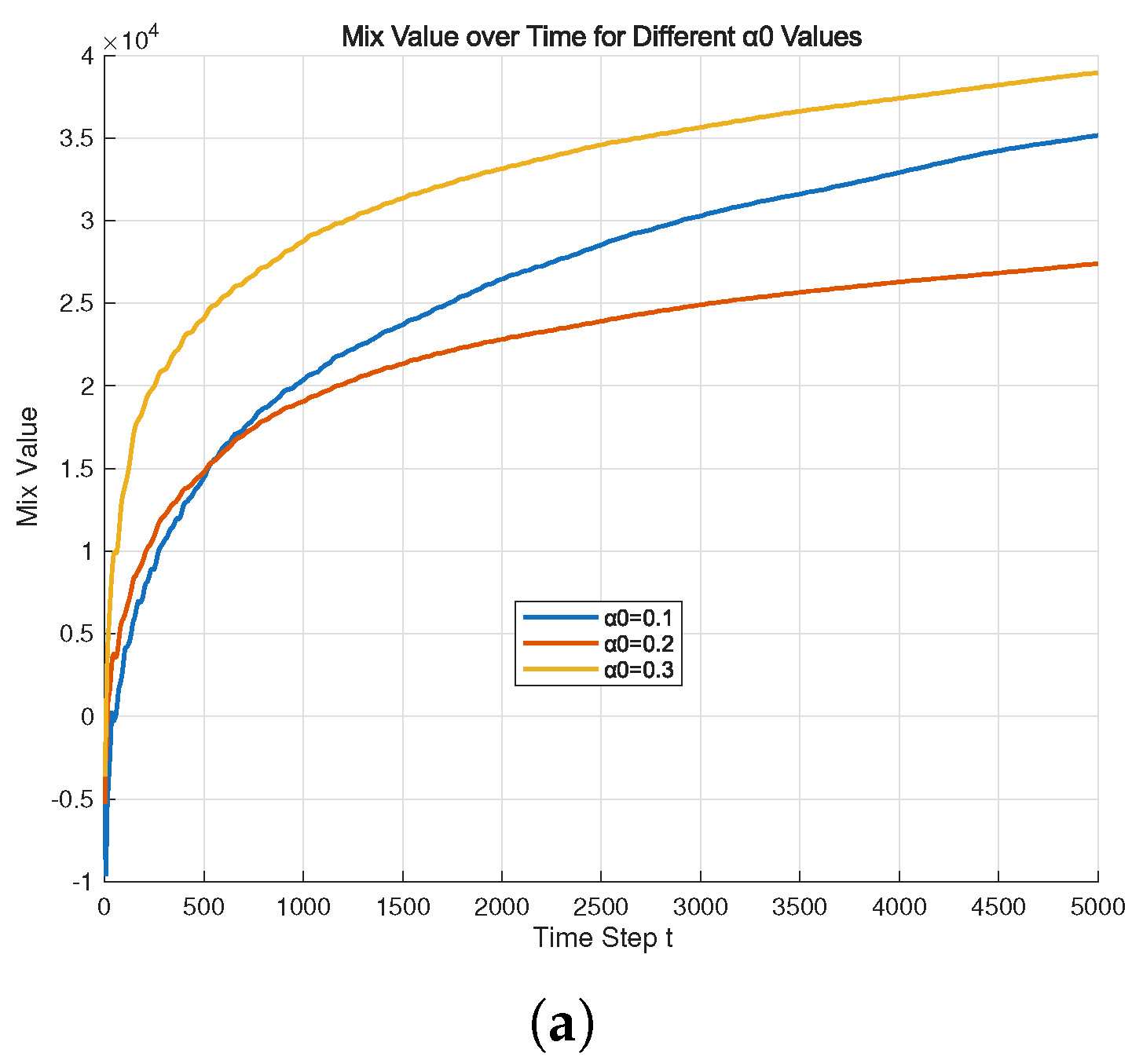
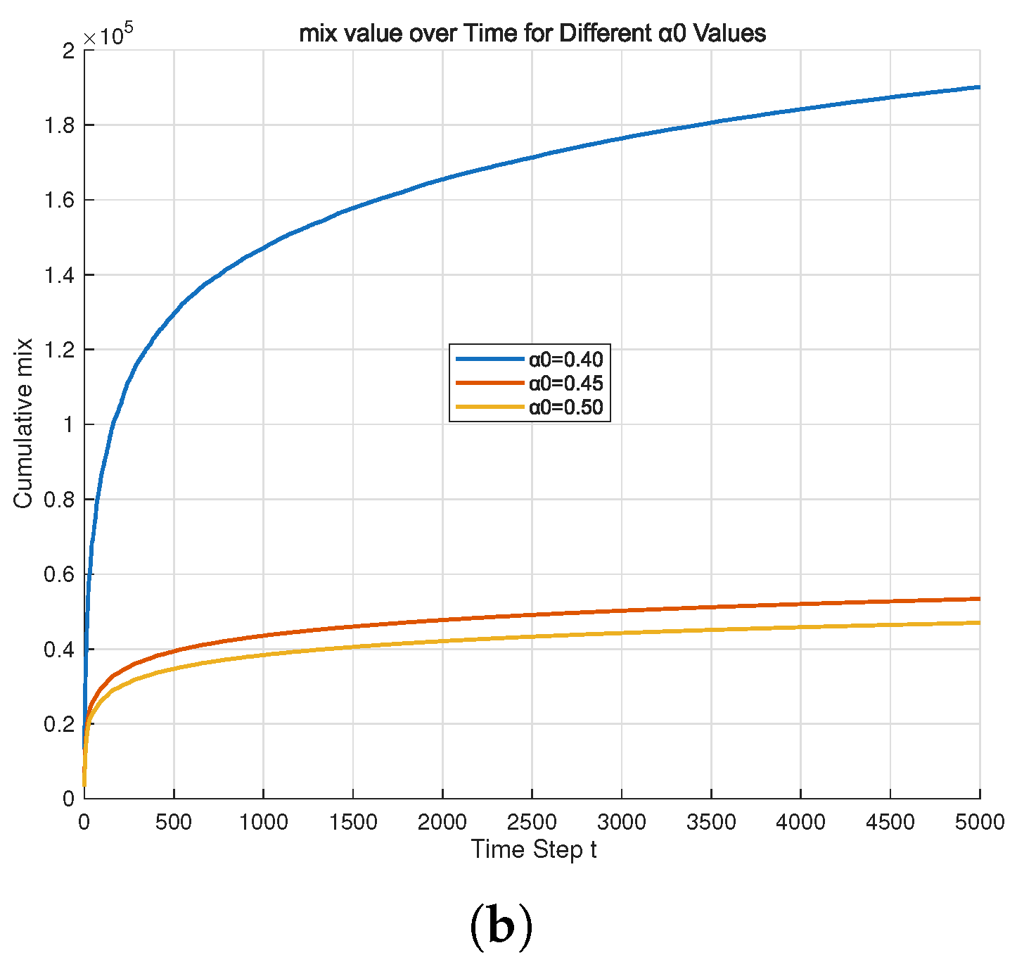
We explored the influence of initial parameter values on our algorithm. Different ${\alpha }_0$ values in our algorithm were compared. There are two criteria for measuring the quality of an online algorithm, so a multi-objective planning approach was adopted to make a mixed measurement. We used the AHP (Analytical Hierarchy Process) to determine the weights of the two quantities. The two measurements correspond to scale value 3 in the 1–9 scale method. So the weight of regret is 0.25, and the weight of constraint violation is 0.75. Our mixed measurement $mix$ is defined as follows:

$$mix=0.25\times regret+0.75\times violation$$

In Figure 1, in adaptive filtering, we found that the algorithm performs the best when ${\alpha }_0=0.2$. And in online logistic regression, the algorithm performs the best when ${\alpha }_0=0.5$.

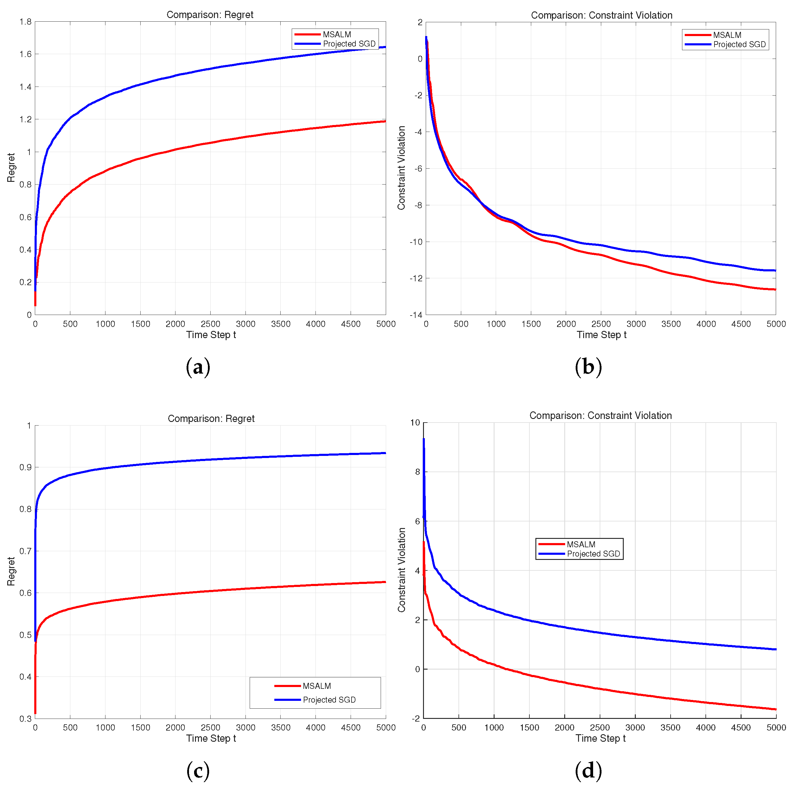
Then we compared our algorithm with the PSGD algorithm. The comparison results are as follows (Figure 2):

We compared the performance of the two algorithms in adaptive filtering and online logistic regression. The figures show that the MSALM attains lower regret and constraint violation bounds than PSGD. This result indicates that our algorithm has the ability to converge more rapidly toward the theoretical optimum while adhering better to the constraints. According to the experimental results, a conclusion can be obtained. When choosing a suitable ${\alpha }_0$, the MSALM is superior to the existing algorithm.

4.2. Experiments Under Existing Models

In order to test the practicality of our algorithm, we applied our algorithm in an energy dispatch problem and network resource allocation.

The time-varying smart grid energy dispatch problem is one of the core tasks of modern smart grids. This problem involves economically and reliably coordinating multiple heterogeneous energy sources while meeting the changing electricity demand. The objective functions of this problem include power balance constraints and resource capacity constraints. The mathematical model of time-varying smart grid energy dispatch is as follows:

$$\underset{x\in {\mathbb{R}}^n}{\min }{c}^{\top }x+{\displaystyle \frac{1}{2}}{x}^{\top }Qx$$

$$\mathrm{s}.\mathrm{t}.{\displaystyle \sum _{i=1}^{n_g}}{x}_i-{\displaystyle \sum _{j=1}^{n_s}}{x}_{n_g+j}-{\displaystyle \sum _{k=1}^{n_d}}{x}_{n_g+n_s+k}=d$$

$$0\le x_i\le u_i,i=1,\dots ,n$$

at each round, c and Q are drawn from independent normal distributions with fixed standard deviations. Their means evolve over time according to a random walk with a decaying step size.

Online network resource allocation is a key challenge in modern computing systems. The key task is to efficiently allocate limited resources to continuously arriving real-time tasks or user requests. We apply our algorithm to a simple network resource allocation problem with link failure to verify its practicality. The network resource allocation problem has the properties of being fully connected, undirected, and static. The objective function consists of two parts: the quality of service cost and resource usage cost. The mathematical model of online network resource allocation is as follows:

$$\underset{x\in {\mathbb{R}}^n}{\min }{\displaystyle \sum _{i=1}^n}{(d_i-x_i)}^2+\alpha {\displaystyle \sum _{i=1}^n}{x}_i$$

$$\mathrm{s}.\mathrm{t}.0\le x_i\le {\tilde{C}}_{t,i},i=1,\dots ,n$$

$${\tilde{C}}_{t,i}=\left\{\begin{array}{cc}0,\hfill & \mathrm{if}\mathrm{link}i\mathrm{fails}\mathrm{at}\mathrm{time}t\hfill \\ C_{t,i},\hfill & \mathrm{otherwise}\hfill \end{array}\right.$$

at each round, the demand vector is drawn from a multivariate normal distribution with fixed standard deviation and truncated to be nonnegative. Its mean vector varies smoothly over time, following a sinusoidal pattern with a slow linear trend. Additionally, each link may fail randomly, forcing its allocated resource to zero; otherwise, its capacity is drawn from a normal distribution with a slowly drifting mean.

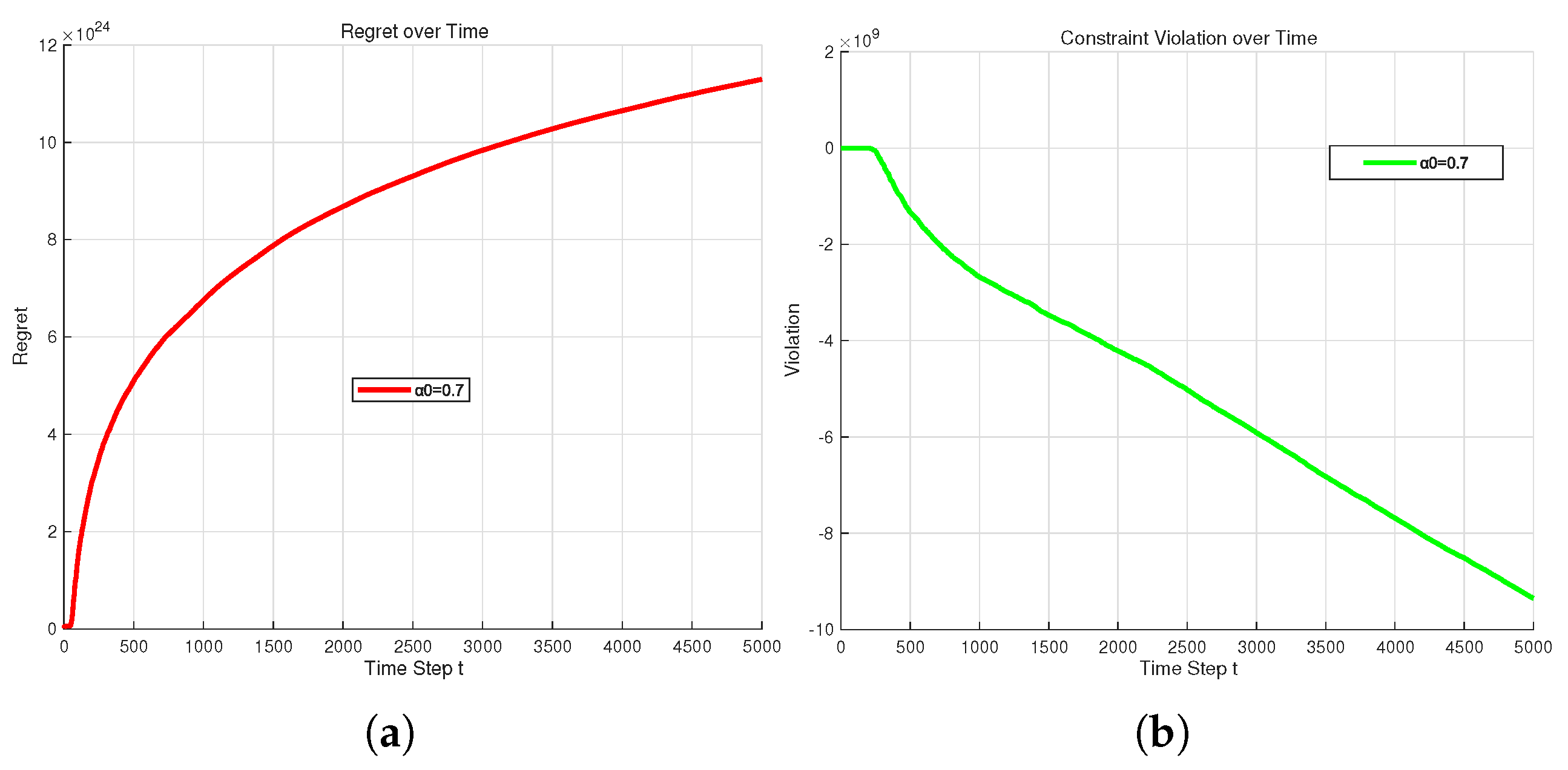
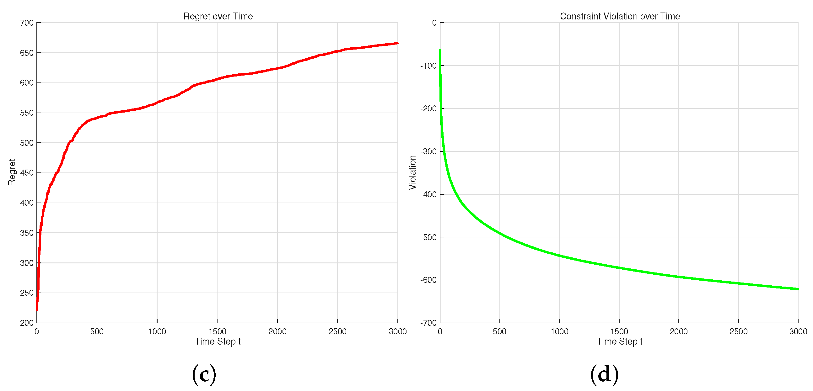
We conducted simulation experiments on two mathematical models, and the results are as follows (Figure 3).

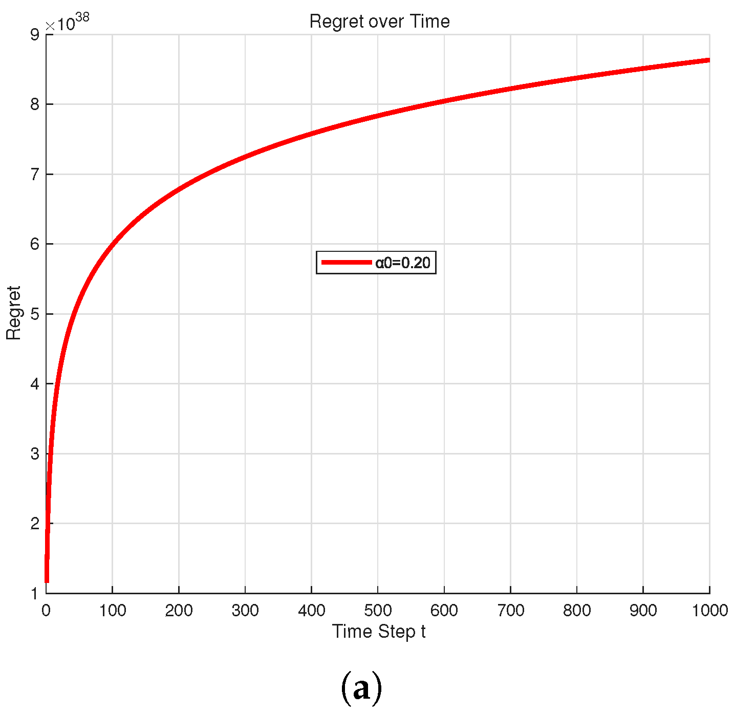
We took ${\alpha }_0=0.7$ and ${\alpha }_0=0.37$ for testing. The simulation experiments show that regret and constraint violation have a sublinear convergent bound of T, demonstrating that our algorithmic solution can gradually approach the theoretically optimal solution while adhering to the constraints. The results show that our algorithm can be applied to the time-varying smart grid energy dispatch problem and the online network resource allocation problem.

4.3. Experiment Combining Our Algorithm with Supervised Learning

We combined the MSALM with supervised learning to solve the path planning problem. To obtain an explicit function that is used in our algorithm, we applied parameter regression methods in supervised learning. First of all, data on 10 flight trajectories for the same flight at the same time slot on different dates were randomly selected. Afterwards, we utilized these data to train a mathematical model for flight trajectories through parameter regression methods. B-spline interpolation was used to obtain the explicit function of the flight trajectory. In order to find the appropriate number of B-spline interpolation control points, we compared the errors between the fitted trajectory and 10 known trajectories under different numbers of control points. We compare the 3D RMSE, mean error, and max error for different numbers of control points. The 3D RMSE reflects the penalty level for large errors and is used to identify and control the severity of extreme deviations. The mean error reflects the typical deviation under normal circumstances and is used to evaluate the fitting accuracy of most trajectory points in daily flights. The max error reflects the deviation limit under the worst-case scenario and is used to evaluate safety margins and risk assessment. The results are as follows (

Table 1. Fitting error with different numbers of control points.

Number of Control Points	3D RMSE (m)	Mean Error (m)	Max Error (m)
6	16,212.93	14,630.05	42,953.94
7	15,278.20	13,697.46	28,088.96
8	10,301.73	9577.57	20,571.04
9	7767.29	7094.96	15,264.24
10	6056.13	5466.36	12,094.13
11	6474.88	5956.19	12,599.98
12	6416.03	5793.27	12,159.70

and

Table 2. Coordinates of control points.

Control Point	X (m)	Y (m)	Z (m)
1	478,288.923	4,423,806.307	1199.714
2	483,007.653	4,412,762.620	1939.867
3	491,176.780	4,411,013.545	1022.683
4	540,450.109	4,386,975.935	6298.608
5	613,313.197	4,283,290.653	6170.731
6	753,322.541	4,268,797.429	6188.807
7	792,318.111	4,171,779.364	6157.780
8	773,451.251	4,061,749.319	3778.580
9	782,481.198	4,033,694.042	2106.506
10	782,988.940	4,014,086.869	1142.003

):

According to the above table, accuracy reaches its highest value when the trajectory has 10 control points. So we obtained the fitting function in this case. The coordinates of the feature points are as follows:

We set some random situations as constraints to simulate the real flight conditions. The constraints include 9 dynamic obstacle avoidance constraints and 4 airspace boundary constraints. The mathematical model of dynamic obstacle avoidance constraints has the following form:

$$g_{k,i}=d_{safe,k}^2(t)-\left|\right|p_i-c_k(t){\left|\right|}^2\le 0$$

where $c_k(t)$ represents the obstacle center coordinates, $d_{safe,k}(t)$ is the safe distance, and $p_i$ is the control point with an obstacle avoidance constraint. We set 3 obstacles and the 1st, 5th, and 10th control points with obstacle avoidance constraints, so $k=1,2,3$ and $i\in \{1,5,10\}$.

The mathematical model of airspace boundary constraints has the following form:

$$x_{min}\le x\le x_{max}$$

$$y_{min}\le y\le y_{max}$$

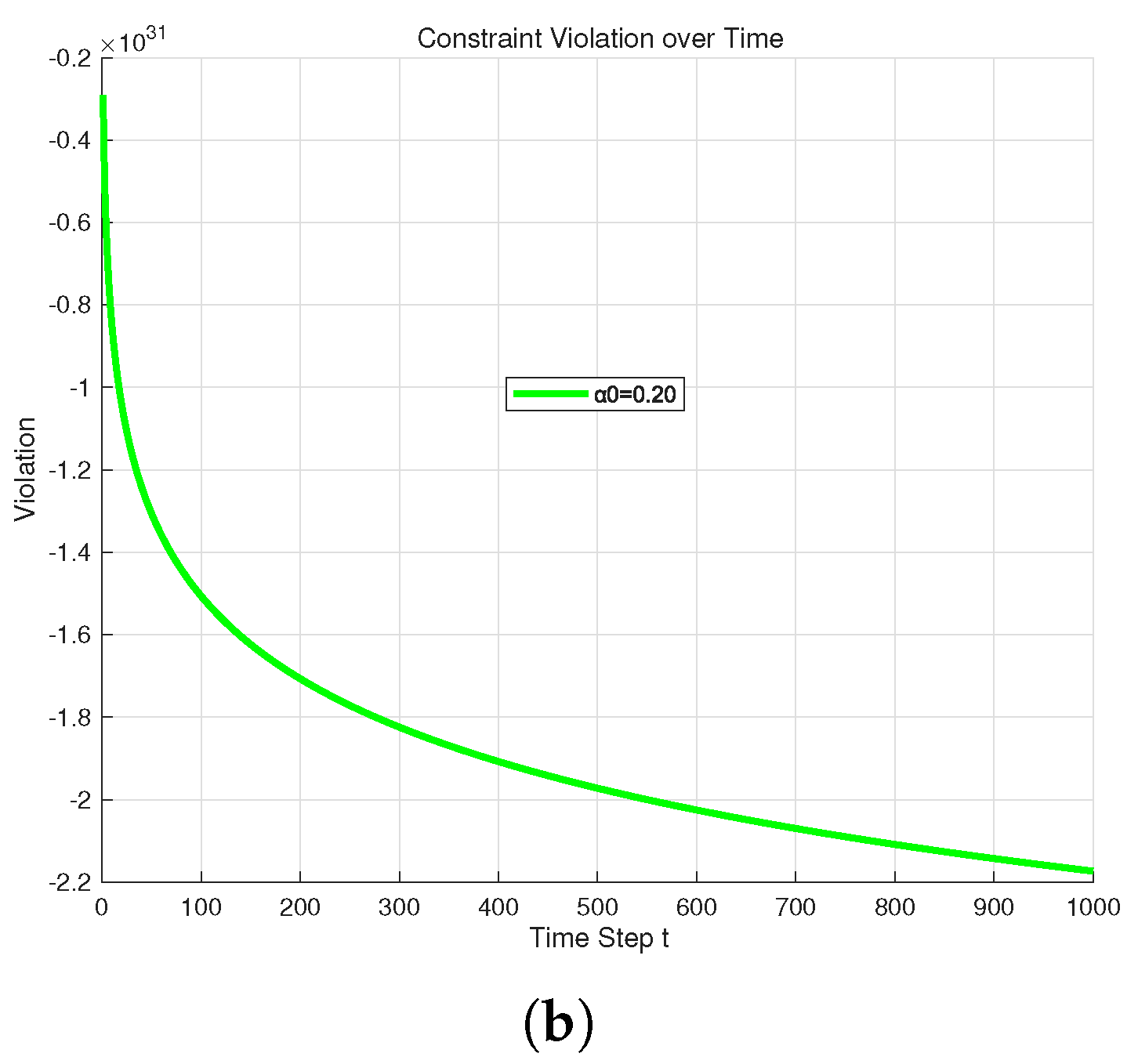
Then we use our algorithm to solve this online optimization problem. The result of the experiment is as follows (Figure 4):

In this figure, the results of the simulation experiment show that the regret and constraint violation of our algorithm have a sublinear convergent bound of T, demonstrating progressive convergence to the theoretical optimum under compliance with the constraint. This indicates that the aircraft can make decisions that gradually approach the optimal choice during the flight and stay as safe as possible in the face of emergencies. This proves that our algorithm can be combined with machine learning methods to be applied to similar path planning problems.

5. Conclusions

In this paper, we present a new online stochastic augmented Lagrangian method, the MSALM, for solving online stochastic optimization problems with time-varying distributions. In each round, we construct model functions for objective and constraint functions based on their properties, which reduces computational complexity. The step size is designed in a dynamic way and decreases as t increases to accelerate convergence. Under standard assumptions, we prove that our algorithm achieves sublinear regret and constraint violation bounds of T. Simulation experiments demonstrate the performance and practical utility of the MSALM algorithm. Additionally, in the context of path planning, we combine our algorithm with supervised learning to further demonstrate its extensibility.