Closed-Form Solutions for the Weibull Distribution Parameters and Performance Lifetime Index with Interval-Censored Data

Abstract

In lifetime testing, reliably assessing the life performance index of the Weibull distribution under Type I interval-censored data is a critical task. Although maximum likelihood estimation (MLE) is a conventional approach for parameter estimation, closed-form solutions are unavailable for this data type. To address this limitation, four least-squares estimation methods based on data transformation are developed. The proposed estimations can provide closed-form solutions for the Weibull distribution and life performance index. The asymptotic unbiasedness and normality of the proposed estimators are rigorously established. Their effectiveness is further supported by simulation studies. Moreover, the practical relevance of the methods is illustrated with two real-data applications.

1. Introduction

In manufacturing, a product’s quality is a critical attribute that attracts considerable attention from both producers and consumers [1]. To assess the product’s quality, the process capability index (PCI) is a simple but widely adopted tool in process capability analysis [2]. Over the years, numerous PCIs have been proposed, among which the life performance index, denoted by $C_L,$ is specifically designed to assess the lifetime performance of electronic components [3]. Because product lifetime is a larger-the-better type of quality characteristic, only the lower specification limit is incorporated in $C_L$. Due to inherent constraints and the asymmetric nature, lifetime data often deviate from normality. Weibull distribution is a particularly important asymmetric distribution in this context, and it has been extensively applied to implement reliability and lifetime analysis. The flexibility of the Weibull distribution in shaping the probability density function (PDF) and its convenient mathematical representation render the Weibull distribution especially effective for modeling lifetime data [4,5,6].

In addition to the lifetime distribution, the method of data collection represents a crucial aspect of lifetime analysis. Owing to constraints of cost, time, and feasibility, it is often impractical to record the exact failure times of items during testing, resulting in observations that are censored in nature [7]. Censoring schemes are thus a common practice in data collection (see Balakrishnan et al. [8], Chapter 1, P.2), with Type I and Type II censoring being the most widely used and conceptually straightforward approaches (see, e.g., [9,10,11,12,13]). Under Type I censoring, exact failure times are observed only up to a prespecified time point, after which subsequent failures are not recorded. In contrast to Type I censoring, Type II censoring terminates the experiment after a prespecified number of failures have occurred. Both Type I and Type II schemes share the feature of continuous monitoring of failure times. However, in certain life-testing scenarios, exact failure times cannot be continuously observed; instead, only the number of failures within predetermined time intervals can be counted. This data collection method is known as the interval-censoring scheme, resulting in interval-censored data. The termination time of such experiments can further give rise to Type I and Type II interval censoring. In Type I interval-censoring, all units are inspected simultaneously at prespecified times (including the termination time), and only the number of failures within consecutive intervals is recorded, instead of the exact failure times, primarily for administrative convenience. The interval-censoring scheme has become increasingly prevalent across engineering [14], biostatistics [15,16], economics [17], and related fields; therefore, it is adopted in the present study.

The life performance index is widely recognized as a numerical measure of process performance and potential, and it has been extensively investigated under different distributional assumptions and censoring schemes [18,19,20,21]. Within the framework of Type I interval censoring, a substantial body of research has explored its applications in diverse fields. These include the design and evaluation of sampling plans [22,23,24,25], system reliability analysis [26,27], model selection [28], hypothesis testing for the mean [29], survival analysis [15], and regression modeling [30,31]. Such studies highlight both the versatility of $C_L$ and the methodological challenges that arise when handling interval-censored data.

Apart from these applications, parameter estimation with Type I interval-censored data has also attracted considerable attention. The classical method MLE has been widely applied in many studies. Recent studies have focused on improving the efficiency of the MLE method. Considering the lower efficiency of MLE with an interval-censoring scheme, Tan [32] proposed a new approach to the Weibull distribution with interval data to improve the efficiency for the MLE problem. Similarly, Wang et al. [33] presented a novel expectation-maximization (EM) algorithm to find the maximum likelihood estimators for interval-censored data. This algorithm is robust to initialization and straightforward to implement. Intuitively, the aforementioned studies do not consider prior information. For this, Ganjali and Baghfalaki [34] constructed a Bayesian method to infer the unemployment duration data. Xu and Wang [35] derived a conjugate prior for the homogeneous gamma process and developed efficient posterior sampling algorithms, significantly improving computational efficiency and estimation accuracy for degradation inference. Furthermore, it extends the conjugate framework to heterogeneous gamma processes and proposes a novel online algorithm that enables recursive parameter updates and effective multi-system remaining useful life prediction. However, the above studies mainly focus on the data with a known distribution. In practice, the distribution of data is usually not fully known. Therefore, nonparametric approaches can be employed to solve the problem. For example, Zeng et al. [36] provided a nonparametric MLE for semiparametric transformation models with interval-censored data; the method converges stably with the existence of time-dependent covariates. The above studies mainly focus on improving efficiency rather than data processing. For this reason, the conditional imputation method [37] and iterative single-point imputation [38] are proposed to address the issues of missing data, improving the performance of censored data, and parameter estimation. Additionally, several studies have compared the efficiency of the MLE and found that it outperforms the naive likelihood estimator [39]. Furthermore, the MLE is usually closer to the best estimator and more robust compared to the minimum distance estimation, ad hoc approach, and imputation method [40].

Although existing studies provide valuable insights, most focus primarily on improving the performance and applications of MLE. Importantly, none of these methods admits closed-form solutions. To provide closed-form solutions, iterative numerical procedures are required, which increase computational complexity, are time-consuming, and are often sensitive to initial values. Consequently, developing a reliable and straightforward parameter estimation method that enables the derivation of closed-form solutions is crucial. In this study, we employ data transformation to construct least-squares estimation (LSE) methods. By converting the PDF into the cumulative distribution function (CDF), a regression framework is established, enabling the application of LSE for parameter estimation and yielding closed-form solutions. Moreover, we derive the statistical properties of the LSE estimators, including asymptotic unbiasedness and normality. Furthermore, we propose an extension of the LSE along with two bias-corrected estimation methods, which not only preserve closed-form solutions but also enhance estimation performance.

The remainder of this paper is organized as follows. Section 2 reviews the life performance index and the MLE method for the Weibull distribution based on Type I interval-censored data. Section 3 presents the proposed LSE methods for the Weibull distribution under Type I interval-censoring, including bias-corrected extensions and their large-sample properties. Section 4 evaluates and compares the performance of the MLE and the proposed methods using Monte Carlo simulations with the absolute bias and mean squared error (MSE) as evaluation metrics. In Section 5, two real-world examples are presented to illustrate the practical applications of the proposed parameter estimation methods. Finally, concluding remarks are provided in Section 6.

2. The Life Performance Index for the Weibull Distribution

Suppose that random variable T follows a Weibull distribution with the shape parameter $k\left(>0\right)$ and scale parameter $\lambda \left(>0\right)$. Denoted it by $T~W\left(k,\lambda \right)$. The PDF and CDF of $W\left(k,\lambda \right)$ are given by

$$f\left(t;k,\lambda \right)={\displaystyle \frac{k}{\lambda }}{\left({\displaystyle \frac{t}{\lambda }}\right)}^{\left(k-1\right)}\mathrm{e}\mathrm{x}\mathrm{p}\left(-{\left({\displaystyle \frac{t}{\lambda }}\right)}^k\right),t\ge 0,$$

(1)

and

$$F\left(t;k,\lambda \right)=1-exp\left(-{\left({\displaystyle \frac{t}{\lambda }}\right)}^k\right),t\ge 0,$$

(2)

respectively. To obtain a reliable life performance index, following Wu and Lin [41], the Weibull data are first transformed into an exponential distribution. Specifically, let $Y=T^k$; then $Y$ follows an exponential distribution with scale parameter $\tilde{\beta }={\lambda }^k$. Defining $\beta =1/\tilde{\beta }$, the PDF and CDF of $Y$ are given by

$$f\left(y;\beta \right)=\beta e^{-\beta y}, y>0,\beta >0,$$

(3)

and

$$F\left(y;\beta \right)=1-e^{-\beta y},y>0,\beta >0,$$

(4)

respectively. The mean and the standard deviation of the variable $Y$ are $\mu =E\left(Y\right)=1/\beta$ and $\sigma =\sqrt{Var\left(Y\right)}=1/\beta$, respectively. The life performance index $C_L$, designed to evaluate larger-the-better quality characteristics, can be defined and presented by

$$C_L={\displaystyle \frac{\mu -L}{\sigma }}={\displaystyle \frac{1/\beta -L}{1/\beta }}=1-\beta L=1-{\displaystyle \frac{L}{{\lambda }^k}},$$

(5)

where $L={\left(L_U\right)}^k$ denotes the known lower specification limit (LSL) of variable $Y$, with $L_U$ being the corresponding LSL of variable $T$. In this study, $L$ is defined as a known constant and does not require estimation. In practice, however, the process parameters are typically unknown and must be estimated. To this end, the conventional MLE method is introduced as follows.

Suppose $n$ units are placed on a life test simultaneously at the initial time; without loss of generality, denote it by $t_0=0$. The units are inspected at $m$ prespecified times $t_1,t_2,\dots ,t_m$, where $t_m$ represents the scheduled termination time of the life test. Let $n_1,n_2,\dots ,n_m$ denote the numbers of units that fail within the intervals (0$,\left.t_1\right],(t_1,\left.t_2\right],\dots ,$ ($t_{\mathrm{m}-1},\left.t_{\mathrm{m}}\right]$, respectively. Define ${\gamma }_i$ as the cumulative number of failures observed up to the i-th intervals, such that ${\gamma }_i={\sum }_{j=1}^i{n}_j$ for $i=1,2,\dots ,m$. At the final inspection time $t_m$, $n-{\gamma }_m$ units remain surviving, which are then treated as censored observations. Accordingly, the likelihood function under Type I interval-censoring is given by

$$\begin{gathered} L\left(\theta \right)\propto {\left(1-F\left(t_m;\theta \right)\right)}^{n-{\gamma }_m}\prod _{i=1}^m{\left(F\left(t_i;\theta \right)-F\left(t_{i-1};\theta \right)\right)}^{n_i} \\ =F{\left(t_1;\theta \right)}^{n_1}{\left[F\left(t_2;\theta \right)-F\left(t_1;\theta \right)\right]}^{n_2}\dots {\left[F\left(t_m;\theta \right)-F\left(t_{m-1};\theta \right)\right]}^{n_m}{\left[1-F\left(t_m;\theta \right)\right]}^{n-\gamma m} \\ ={\left[1-\exp \left(-{\left({\displaystyle \frac{t_1}{\lambda }}\right)}^k\right)\right]}^{n_1}{\left[\exp \left(-{\left({\displaystyle \frac{t_1}{\lambda }}\right)}^k\right)-\exp \left(-{\left({\displaystyle \frac{t_2}{\lambda }}\right)}^k\right)\right]}^{n_2}\dots {\left[\exp \left(-{\left({\displaystyle \frac{t_{m-1}}{\lambda }}\right)}^k\right)-\exp \left(-{\left({\displaystyle \frac{t_m}{\lambda }}\right)}^k\right)\right]}^{n_m}\exp \left(-{\left({\displaystyle \frac{t_m}{\lambda }}\right)}^k·\left(n-{\gamma }_m\right)\right), \end{gathered}$$

(6)

where $\mathit{\theta }=$ ($k,\lambda$). The MLE of $\mathit{\theta }$, denoted as ${\widehat{\mathit{\theta }}}_{\mathit{M}\mathit{L}\mathit{E}}=$ (${\widehat{k}}_{MLE},{\widehat{\lambda }}_{MLE}$), is obtained by maximizing the log-likelihood function. The term MLE is used to denote the maximum likelihood estimation and the maximum likelihood estimate hereafter. Unfortunately, ${\widehat{\mathit{\theta }}}_{\mathit{M}\mathit{L}\mathit{E}}$ does not admit closed-form solutions and must be computed using numerical methods, which poses challenges for practical implementation. By substituting $\mathit{\theta }$ with ${\widehat{\mathit{\theta }}}_{\mathit{M}\mathit{L}\mathit{E}}$ in Equation (5), the MLE of the life performance index $C_L$ is expressed as

$${\widehat{C}}_{L,MLE}=1-L/{{\widehat{\lambda }}_{MLE}}^{{\widehat{k}}_{MLE}}.$$

(7)

3. Proposed Estimation Methods

3.1. Least-Squares Estimation Methods

Suppose the random variable $T~W\left(k,\lambda \right)$ and define $U^{*}=F\left(T;k,\lambda \right)$. Then, $U^{*}~U\left(0,1\right)$, where $U\left(0,1\right)$ denotes the uniform distribution on the interval $(0,1)$. In the case of complete samples, let $l_i~W\left(k,\lambda \right)$ be independent and identically distributed (i.i.d), and define $U_i=F\left(l_i;\mathsf{\Theta }\right)$ for $i=1,2,\dots ,n$. It follows that $U_i~U\left(0,1\right)$. Furthermore, let the vector $U_v=(U_{1:n},U_{2:n},\dots ,U_{n:n})$ denote the order statistics from $U\left(0,1\right)$, where the i-th element is $U_{i:n}$. Consequently, $U_{i:n}$ follows a Beta distribution with shape parameters $i$ and $n-i+1$, i.e., $U_{i:n}~Beta\left(i,n-i+1\right)$ for $i=1,2,\dots ,n$. The mean of $U_{i:n}$, also referred to as the mean rank, is given by

$$E\left(U_{i:n}\right)={\displaystyle \frac{i}{n+1}}.$$

(8)

When the data collected is subject to the Type I interval-censoring scheme, the exact failure times of individual units are unobservable. Nevertheless, the probability of failure prior to $t_i$ can be expressed as

$$P\left(T<t_i\right)=P\left(U^{*}<F\left(t_i;\mathsf{\Theta }\right)\right),i=1,2,\dots ,m.$$

(9)

Furthermore, if ${\gamma }_i$ units fail earlier than $t_i$, it follows that $t_i$ lies between the survival times of the ${{\gamma }_i}^{\mathrm{t}\mathrm{h}}$ and ${({\gamma }_i+1)}^{\mathrm{t}\mathrm{h}}$ units. Denote the failure times of the ${{\gamma }_i}^{\mathrm{t}\mathrm{h}}$ and ${({\gamma }_i+1)}^{\mathrm{t}\mathrm{h}}$ units by $t_{\left({\gamma }_i\right)}$ and $t_{({\gamma }_i+1)}$, respectively. Accordingly, we obtain the following expression:

$$\begin{gathered} P\left(U^{*}<F\left(t_{\left({\gamma }_i\right)};\mathsf{\Theta }\right)\right)<P\left(U^{*}<F\left(t_i;\mathsf{\Theta }\right)\right)<P\left(U^{*}<F\left(t_{({\gamma }_i+1)};\mathsf{\Theta }\right)\right) \\ \Rightarrow P\left(U^{*}<F\left(t_{\left({\gamma }_i\right)};\mathsf{\Theta }\right)\right)<1-\exp \left(-{\left({\displaystyle \frac{t_i}{\lambda }}\right)}^k\right)<P\left(U^{*}<F\left(t_{\left({\gamma }_i+1\right)};\mathsf{\Theta }\right)\right), \\ i=1,2,\dots ,m. \end{gathered}$$

(10)

To estimate the values of the cumulative distribution function $P\left(U^{*}<F\left(t_{\left({\gamma }_i\right)};\mathsf{\Theta }\right)\right)$, we employ the cumulative mean rank, expressed as:

$$\widehat{P}\left(U^{*}<F\left(t_{\left({\gamma }_i\right)};\mathsf{\Theta }\right)\right)={\displaystyle \frac{{\gamma }_i}{n+1}},i=1,2,\dots ,m.$$

(11)

Equation (10) can be rewritten as

$${\displaystyle \frac{{\gamma }_i}{n+1}}<1-\mathrm{e}\mathrm{x}\mathrm{p}\left(-{\left({\displaystyle \frac{t_i}{\lambda }}\right)}^k\right)<{\displaystyle \frac{{\gamma }_i+1}{n+1}},i=1,2,\dots ,m.$$

(12)

To facilitate a straightforward estimation of the parameters in Equation (12), we can use the midpoint of the interval for the approximation:

$$1-\exp \left(-{\left({\displaystyle \frac{t_i}{\lambda }}\right)}^k\right)\approx {\displaystyle \frac{1}{2}}\left({\displaystyle \frac{{\gamma }_i}{n+1}}+{\displaystyle \frac{{\gamma }_i+1}{n+1}}\right)={\displaystyle \frac{2{\gamma }_i+1}{2\left(n+1\right)}},i=1,2,\dots ,m.$$

(13)

Furthermore, by applying the logarithm twice to Equation (13), we obtain

$$Y_i={\beta }_0+{\beta }_1{X}_i,i=1,2,\dots ,m,$$

(14)

where $Y_i=\mathrm{l}\mathrm{n}\left[-\mathrm{l}\mathrm{n}\left(1-{\displaystyle \frac{2{\gamma }_i+1}{2\left(n+1\right)}}\right)\right]$, $X_i=\mathrm{l}\mathrm{n}\left(t_i\right)$, ${\beta }_0=-k\mathrm{l}\mathrm{n}\left(\lambda \right)$ and ${\beta }_1=k$, $i=1,2,\dots ,m$. The estimators ${\widehat{\beta }}_0$ and ${\widehat{\beta }}_1$ of the regression parameters ${\beta }_0$ and ${\beta }_1$ are given by

$${\widehat{\beta }}_1={\displaystyle \frac{m{\sum }_{i=1}^m\ln \left(t_i\right)\mathrm{l}\mathrm{n}\left[-\ln \left(1-p_i\right)\right]-{\sum }_{i=1}^m\ln \left(t_i\right){\sum }_{i=1}^m\mathrm{l}\mathrm{n}\left[-\ln \left(1-p_i\right)\right]}{m{\sum }_{i=1}^m{\mathrm{l}\mathrm{n}}^2\left(t_i\right)-{\left({\sum }_{i=1}^m\mathrm{l}\mathrm{n}\left(t_i\right)\right)}^2}}$$

(15)

and

$${\widehat{\beta }}_0={\displaystyle \frac{1}{m}}{\sum }_{i=1}^m\mathrm{l}\mathrm{n}\left[-\ln \left(1-p_i\right)\right]-{\widehat{\beta }}_1{\displaystyle \frac{1}{m}}{\sum }_{i=1}^m\ln \left(t_i\right),$$

(16)

where $p_i={\displaystyle \frac{2{\gamma }_i+1}{2\left(n+1\right)}}$. The term LSE is used to denote the least-squares estimation, and the least-squares estimate hereafter. The LSEs of the parameters $k$ and $\lambda$ are given by

$${\widehat{k}}_{LSE}={\widehat{\beta }}_1,$$

(17)

and

$${\widehat{\lambda }}_{LSE}=\mathrm{e}\mathrm{x}\mathrm{p}\left(-{\displaystyle \frac{{\sum }_{i=1}^m\mathrm{l}\mathrm{n}\left[-\ln \left(1-p_i\right)\right]-{\widehat{k}}_{LSE}{\sum }_{i=1}^m\ln \left(t_i\right)}{m{\widehat{k}}_{LSE}}}\right),$$

(18)

respectively. Replacing $\mathit{\theta }$ with ${\widehat{\mathit{\theta }}}_{\mathit{L}\mathit{S}\mathit{E}}=({\widehat{k}}_{LSE},{\widehat{\lambda }}_{LSE})$ in Equation (5), the LSE of the life performance index $C_L$ is given b

$${\widehat{C}}_{L,LSE}=1-L/{{\widehat{\lambda }}_{LSE}}^{{\widehat{k}}_{LSE}}.$$

(19)

As m increases, the probability of sample-free observation intervals also rises, which reduces the estimation efficiency of the LSE method. To improve estimation performance, a method that applies LSE after removing intervals with no observations is defined as PLSE. The corresponding parameter is denoted by ${\widehat{\mathit{\theta }}}_{\mathit{P}\mathit{L}\mathit{S}\mathit{E}}=({\widehat{k}}_{PLSE},{\widehat{\lambda }}_{PLSE})$. Consequently, the PLSE of $C_L$ is given by

$${\widehat{C}}_{L,PLSE}=1-L/{{\widehat{\lambda }}_{PLSE}}^{{\widehat{k}}_{PLSE}}.$$

(20)

We further examined the large-sample properties of the proposed estimators, from which the following results are established.

Theorem 1.

Let $t_j, j=1,2,\cdots ,n$ be i.i.d. random variables from $W\left(k_0,{\lambda }_0\right)$, and let ${\tau }_i,i=1,2,\cdots ,m$ denote predetermined time points. Suppose that ${\gamma }_i (i=1,2,\dots ,m)$ units fail earlier than $t_i$ . Then, the parameter estimators in Equations (17) and (18) satisfy

$$\underset{n\to \infty }{plim} {\widehat{k}}_{LSE}=k_0,$$

$$\underset{n\to \infty }{plim} {\widehat{\lambda }}_{LSE}={\lambda }_0.$$

Theorem 2.

The parameter estimators in Equations (17) and (18) satisfy

$$\sqrt{n}\left({\widehat{k}}_{LSE}-k_0\right)\stackrel{\hspace{1em}d\hspace{1em}}{\to }N\left(0,{A_0}^{\prime }{\Sigma }_p{A}_0\right),$$

$$\sqrt{n}\left({\widehat{\lambda }}_{LSE}-{\lambda }_0\right)\stackrel{\hspace{1em}d\hspace{1em}}{\to }N\left(0,{B_0}^{\prime }{\Sigma }_p{B}_0\right),$$

 where

$$A_0={\displaystyle \frac{mS-{\sum }_{i=1}^m\mathit{ln}\left({\tau }_i\right)Q}{m{\sum }_{i=1}^m{\mathit{ln}}^2\left({\tau }_i\right)-{\left({\sum }_{i=1}^m{\mathit{ln}}^2\left({\tau }_i\right)\right)}^2}},B_0={\displaystyle \frac{{\lambda }_0}{mk}}\left(A_0{\sum }_{i=1}^m\mathit{ln}\left({\displaystyle \frac{{\tau }_i}{{\lambda }_0}}\right)-Q\right),$$

$${\Sigma }_p={\left({\Sigma }_{il}\right)}_{m\times m},$$

$${\Sigma }_{il}={\Sigma }_{li}=\mathit{exp}\left(-{\left({\displaystyle \frac{{\tau }_i}{{\lambda }_0}}\right)}^{k_0}\right)\left[1-\mathit{exp}\left(-{\left({\displaystyle \frac{{\tau }_i}{{\lambda }_0}}\right)}^{k_0}\right)\right],i\le l,$$

$$S={\left(s_1,s_2,\cdots ,s_m\right)}^{\prime },s_i=\mathit{ln}\left({\tau }_i\right)q_i,i=1,2,\cdots ,m,$$

$$Q={\left(q_1,q_2,\cdots ,q_m\right)}^{\prime },q_i=-{\mathit{exp}\left({\displaystyle \frac{{\tau }_i}{{\lambda }_0}}\right)}^{k_0}{\left({\displaystyle \frac{{\lambda }_0}{{\tau }_i}}\right)}^{k_0},i=1,2,\cdots ,m.$$

Then, ${\widehat{k}}_{LSE}$ and ${ \widehat{\lambda }}_{LSE}$ are consistent estimators of the parameters $k_0$ and ${\lambda }_0$ and possess asymptotic normality. Similarly, the improved estimators ${\widehat{k}}_{PLSE}$ and ${\widehat{\lambda }}_{PLSE}$ exhibit the same properties. The proofs of Theorems 1 and 2 are provided in the Appendix A.

3.2. Bias-Corrected Least-Squares Estimation Methods

Although the estimators ${\widehat{\mathit{\theta }}}_{\mathit{L}\mathit{S}\mathit{E}}$ and ${\widehat{\mathit{\theta }}}_{\mathit{P}\mathit{L}\mathit{S}\mathit{E}}$ are consistent, they may exhibit bias in finite samples. To enhance their performance, bias correction is implemented using Efron’s [42] bootstrap resampling method. The idea of this method is to generate pseudo-samples from the original data to estimate the bias of the estimator and then subtract the estimated bias from the original estimator to obtain the bias-corrected estimator.

Specifically, let $\left(t_i,n_i\right)$, $i=1,2,\dots ,m$, denote a Type I interval-censored sample drawn from $T~W\left(k,\lambda \right)$. The LSE method is applied to estimate parameters and the resulting LSE is denoted by ${\widehat{\mathit{\theta }}}_{\mathit{L}\mathit{S}\mathit{E}}=\left({\widehat{k}}_{LSE},{\widehat{\lambda }}_{LSE}\right)$. $B$ pseudo-samples can be generated from the $W\left({\widehat{k}}_{LSE},{\widehat{\lambda }}_{LSE}\right)$ distribution based on $B$ repetitions of same size. In each repetition, the LSEs of $k$ and $\lambda$ are estimated using the generated pseudo-sample and the resulting LSE is denoted by ${\widehat{\mathit{\theta }}}_{\mathit{B}\mathit{o}\mathit{o}\mathit{t}}^{\mathit{L}\mathit{S}\mathit{E}}=\left({\widehat{\mathit{k}}}_{\mathit{B}\mathit{o}\mathit{o}\mathit{t}}^{\mathit{L}\mathit{S}\mathit{E}},{\widehat{\mathit{\lambda }}}_{\mathit{B}\mathit{o}\mathit{o}\mathit{t}}^{\mathit{L}\mathit{S}\mathit{E}}\right)$, where ${\widehat{\mathit{k}}}_{\mathit{B}\mathit{o}\mathit{o}\mathit{t}}^{\mathit{L}\mathit{S}\mathit{E}}=\left\{{\widehat{k}}_{LSE,1},{\widehat{k}}_{LSE,2},\dots ,{\widehat{k}}_{LSE,B}\right\}$, ${\widehat{\mathit{\lambda }}}_{\mathit{B}\mathit{o}\mathit{o}\mathit{t}}^{\mathit{L}\mathit{S}\mathit{E}}=\left\{{\widehat{\lambda }}_{LSE,1},{\widehat{\lambda }}_{LSE,2},\dots ,{\widehat{\lambda }}_{LSE,B}\right\}.$ $B$ is a large positive integer. Correspondingly, the life performance index $C_L$ based on the bootstrap samples can be expressed as ${{\widehat{C}}_L}_{\mathit{B}\mathit{o}\mathit{o}\mathit{t}}^{\mathit{L}\mathit{S}\mathit{E}}$, where ${{\widehat{C}}_L}_{\mathit{B}\mathit{o}\mathit{o}\mathit{t}}^{\mathit{L}\mathit{S}\mathit{E}}=1-L/{{\widehat{\mathit{\lambda }}}_{\mathit{B}\mathit{o}\mathit{o}\mathit{t}}^{\mathit{L}\mathit{S}\mathit{E}}}^{{\widehat{\mathit{k}}}_{\mathit{B}\mathit{o}\mathit{o}\mathit{t}}^{\mathit{L}\mathit{S}\mathit{E}}}$ and ${{\widehat{C}}_L}_{\mathit{B}\mathit{o}\mathit{o}\mathit{t}}^{\mathit{L}\mathit{S}\mathit{E}}=\{{\widehat{C}}_{L,LSE,1},{\widehat{C}}_{L,LSE,2},\dots ,{\widehat{C}}_{L,LSE,B}\}$.

Thus, the bootstrap estimate of the bias can be obtained as follows:

$$\widehat{\mathit{B}\mathit{B}}=E\left({\widehat{\mathit{\theta }}}_{\mathit{B}\mathit{o}\mathit{o}\mathit{t}}^{\mathit{L}\mathit{S}\mathit{E}}\right)-{\widehat{\mathit{\theta }}}_{\mathit{L}\mathit{S}\mathit{E}};\widehat{BBC}=E\left({{\widehat{C}}_L}_{\mathit{B}\mathit{o}\mathit{o}\mathit{t}}^{\mathit{L}\mathit{S}\mathit{E}}\right)-{\widehat{C}}_{L,LSE},$$

(21)

In this paper, we consider the expected values of ${\widehat{\mathit{\theta }}}_{\mathit{B}\mathit{o}\mathit{o}\mathit{t}}^{\mathit{L}\mathit{S}\mathit{E}}$ and ${{\widehat{C}}_L}_{\mathit{B}\mathit{o}\mathit{o}\mathit{t}}^{\mathit{L}\mathit{S}\mathit{E}}$ to be

$$\begin{gathered} E\left({\widehat{\mathit{\theta }}}_{\mathit{B}\mathit{o}\mathit{o}\mathit{t}}^{\mathit{L}\mathit{S}\mathit{E}}\right)\cong \left({\displaystyle \frac{1}{B}}\sum _{i=1}^B{\widehat{k}}_{LSE,i},{\displaystyle \frac{1}{B}}\sum _{i=1}^B{\widehat{\lambda }}_{LSE,i}\right); \\ E\left({{\widehat{C}}_L}_{\mathit{B}\mathit{o}\mathit{o}\mathit{t}}^{\mathit{L}\mathit{S}\mathit{E}}\right)\cong {\displaystyle \frac{1}{B}}\sum _{i=1}^B{\widehat{C}}_{L,LSE,i}. \end{gathered}$$

(22)

Accordingly, the bias-corrected least squares estimators of $\mathit{\theta }$ and $C_L$ are given by:

$$\begin{gathered} {\widehat{\mathit{\theta }}}_{\mathit{C}\mathit{L}\mathit{S}\mathit{E}}=\left({\widehat{k}}_{CLSE},{\widehat{\lambda }}_{CLSE}\right)={\widehat{\mathit{\theta }}}_{\mathit{L}\mathit{S}\mathit{E}}-\widehat{\mathit{B}\mathit{B}}=\mathbf{2}{\widehat{\mathit{\theta }}}_{\mathit{L}\mathit{S}\mathit{E}}-E\left({\widehat{\mathit{\theta }}}_{\mathit{B}\mathit{o}\mathit{o}\mathit{t}}^{\mathit{L}\mathit{S}\mathit{E}}\right), \\ {\widehat{C}}_{L,CLSE}={\widehat{C}}_{L,LSE}-\widehat{BBC}=2{\widehat{C}}_{L,LSE}-E\left({{\widehat{C}}_L}_{\mathit{B}\mathit{o}\mathit{o}\mathit{t}}^{\mathit{L}\mathit{S}\mathit{E}}\right). \end{gathered}$$

(23)

The algorithm for implementing the bias-corrected LSE is presented as follows:

• Based on the Type-I interval-censored sample $(t_i,n_i)$, $i=1,2,\dots ,m$, the LSE ${\widehat{\mathit{\theta }}}_{\mathit{L}\mathit{S}\mathit{E}}=\left({\widehat{k}}_{LSE},{\widehat{\lambda }}_{LSE}\right)$ is obtained based on this sample.
• Generate a pseudo-sample of size n from the Weibull distribution with shape parameter ${\widehat{k}}_{LSE}$ and scale parameter ${\widehat{\lambda }}_{LSE}$.
• Transform the generated pseudo-sample into a Type I interval-censored sample based on $t_1,t_2,\dots ,t_m$, denoted as a Type-I interval pseudo-sample.
• Compute the LSEs of k, $\lambda$, and $C_L$ using this Type-I interval pseudo-sample.
• Repeat Step 2 to Step 4 $B$ times to obtain two sets of size $B$ estimators, i.e., ${\widehat{\mathit{\theta }}}_{\mathit{B}\mathit{o}\mathit{o}\mathit{t}}^{\mathit{L}\mathit{S}\mathit{E}}$ and ${{\widehat{C}}_L}_{\mathit{B}\mathit{o}\mathit{o}\mathit{t}}^{\mathit{L}\mathit{S}\mathit{E}}$
• Calculate the $E\left({\widehat{\mathit{\theta }}}_{\mathit{B}\mathit{o}\mathit{o}\mathit{t}}^{\mathit{L}\mathit{S}\mathit{E}}\right)$ and $E\left({{\widehat{C}}_L}_{\mathit{B}\mathit{o}\mathit{o}\mathit{t}}^{\mathit{L}\mathit{S}\mathit{E}}\right)$ according to the Equation (22).
• Using Equation (22), the bias-corrected LSEs of k, $\lambda$ and $C_L$ are computed as ${\widehat{k}}_{CLSE}=2{\widehat{k}}_{LSE}-{\displaystyle \frac{1}{B}}\sum _{i=1}^B{\widehat{k}}_{LSE,i}$, ${\widehat{\lambda }}_{CLSE}=2{\widehat{\lambda }}_{LSE}-{\displaystyle \frac{1}{B}}\sum _{i=1}^B{\widehat{\lambda }}_{LSE,i}$ and ${\widehat{C}}_{L,CLSE}=2{\widehat{C}}_{L,LSE}-{\displaystyle \frac{1}{B}}\sum _{i=1}^B{\widehat{C}}_{L,LSE,i}$.

Similarly, by replacing the LSE method in the above steps with the PLSE method, we obtain the bias-corrected PLSE estimators, denoted by ${\widehat{k}}_{CPLSE}$, ${\widehat{\lambda }}_{CPLSE}$ and ${\widehat{C}}_{L,CPLSE}$. For the sake of brevity, the details are omitted here.

4. Simulation Study

This section presents numerical simulations designed to evaluate the performance of the proposed LSEs. First, we compare the efficiency of MLE with that of the LSE and PLSE. Next, to assess the impact of the bias-correction procedure, we report the simulation results obtained from the bias-corrected versions of the LSE and PLSE. All simulations are conducted using 10,000 Monte Carlo replications. The comparisons are based on two criteria: the absolute bias ($A_b$) and the mean squared error (MSE), whose mathematical formulations are provided below.

$$A_b=\left|{\displaystyle \frac{1}{\mathrm{10,000}}}{\sum }_{i=1}^{\mathrm{10,000}}({\vartheta }_j-{\widehat{\vartheta }}_j)\right|,$$

(24)

and

$$MSE={\displaystyle \frac{1}{\mathrm{10,000}}}{\sum }_{i=1}^{\mathrm{10,000}}{\left({\vartheta }_j-{\widehat{\vartheta }}_j\right)}^2,$$

(25)

where ${\widehat{\vartheta }}_j$ denotes $\widehat{k},\widehat{\lambda },$ and ${\widehat{C}}_L$ corresponding to $j=1,2,3$, with ${\vartheta }_j$ representing the true parameters $k,\lambda ,$ and $C_L$ for $j=1,2,3$. Here, ${\widehat{\vartheta }}_j$ stands for the estimators of ${\vartheta }_j$, including the MLE, LSE, PLSE, and the bias-corrected versions of LSE and PLSE. The data for the experimental design are randomly generated from the Weibull distribution with parameter settings $\left(k,\lambda \right)=\left(1,1\right),\left(2,1\right),\left(3,1\right)$. Following Hu and Gui [18], and Wu and Lin [41], the sample sizes are set to $n=20,30,50,100$, with a lower specification limit of $L=0.05$ and interval numbers $m=3,5,10$. The corresponding inspection time points for each case are summarized in

Table 1. Observation time in different groups.

Sample Sizes and Interval Numbers	Cases
$m=3$ $n=20,30,50$	$Case1:T=\left(0.2,0.7,1.2\right);Case2:T=\left(0.4,0.9,1.4\right);$ $Case3:T=\left(0.2,1.0,1.8\right);Case4:T=\left(0.2,0.7,1.5\right);$ $Case5:T=(0.2,1.0,1.5);$
$m=5$ $n=20,30,50$	$Case6:T=\left(0.2,0.5,0.8,1.1,1.4\right);$ $Case7:T=\left(0.4,0.7,1.0,1.3,1.6\right);$ $Case8:T=\left(0.2,0.6,1.0,1.4,1.8\right);$ $Case9:T=\left(0.2,0.4,0.7,1.1,1.6\right);$ $Case10:T=\left(0.2,0.5,1.0,1.5,1.8\right);$
$m=10$ $n=30,50,100$	$Case11:T=\left(0.1,0.3,0.5,0.7,0.9,1.1,1.3,1.5,1.7,1.9\right);$ $Case12:T=\left(0.3,0.5,0.7,0.9,1.1,1.3,1.5,1.7,1.9,2.1\right);$ $Case13:T=\left(0.1,0.4,0.7,1.0,1.3,1.6,1.9,2.2,2.5,2.8\right);$ $Case14:T=\left(0.1,0.15,0.25,0.4,0.6,0.85,1.15,1.5,1.9,2.35\right);$ $Case15:T=\left(0.1,0.15,0.25,0.4,0.6,0.85,1.05,1.2,1.3,1.35\right);$

. The code of the proposed method can be found at https://github.com/Zhengcheng11/Code-of-the-LSE-and-PLSE (accessed on 19 December 2025).

The simulation results are presented in

Table 2. Type I interval-censored with $m=3$.

			MLE						LSE						PLSE
			${\widehat{\mathit{k}}}_{\mathit{M}\mathit{L}\mathit{E}}$		${\widehat{\mathit{\lambda }}}_{\mathit{M}\mathit{L}\mathit{E}}$		${\widehat{\mathit{C}}}_{\mathit{L},\mathit{M}\mathit{L}\mathit{E}}$		${\widehat{\mathit{k}}}_{\mathit{L}\mathit{S}\mathit{E}}$		${\widehat{\mathit{\lambda }}}_{\mathit{L}\mathit{S}\mathit{E}}$		${\widehat{\mathit{C}}}_{\mathit{L},\mathit{L}\mathit{S}\mathit{E}}$		${\widehat{\mathit{k}}}_{\mathit{P}\mathit{L}\mathit{S}\mathit{E}}$		${\widehat{\mathit{\lambda }}}_{\mathit{P}\mathit{L}\mathit{S}\mathit{E}}$		${\widehat{\mathit{C}}}_{\mathit{L},\mathbf{P}\mathit{L}\mathit{S}\mathit{E}}$
$\mathit{k}$	$\mathit{n}$	$\mathit{C}\mathit{a}\mathit{s}\mathit{e}$	${\mathit{A}}_{\mathit{b}}$	$\mathit{M}\mathit{S}\mathit{E}$	${\mathit{A}}_{\mathit{b}}$	$\mathit{M}\mathit{S}\mathit{E}$	${\mathit{A}}_{\mathit{b}}^{\mathit{*}}$	${\mathit{M}\mathit{S}\mathit{E}}^{\mathit{*}}$	${\mathit{A}}_{\mathit{b}}$	$\mathit{M}\mathit{S}\mathit{E}$	${\mathit{A}}_{\mathit{b}}$	$\mathit{M}\mathit{S}\mathit{E}$	${\mathit{A}}_{\mathit{b}}^{\mathit{*}}$	${\mathit{M}\mathit{S}\mathit{E}}^{\mathit{*}}$	${\mathit{A}}_{\mathit{b}}$	$\mathit{M}\mathit{S}\mathit{E}$	${\mathit{A}}_{\mathit{b}}$	$\mathit{M}\mathit{S}\mathit{E}$	${\mathit{A}}_{\mathit{b}}^{\mathit{*}}$	${\mathit{M}\mathit{S}\mathit{E}}^{\mathit{*}}$
1	20	1	0.07	0	0.06	0	0.2	0.04	0	0	0.1	0.01	0.09	0.01	0.01	0	0.1	0.01	0.12	0.01
		2	0.05	0	0.06	0	0.21	0.04	0.01	0	0.14	0.02	0.08	0.01	0	0	0.09	0.01	0.13	0.02
		3	0.07	0	0.03	0	0.17	0.03	0.01	0	0.05	0	0.06	0	0.02	0	0.04	0	0.1	0.01
		4	0.06	0	0.04	0	0.19	0.04	0	0	0.07	0	0.07	0	0.02	0	0.07	0.01	0.08	0.01
		5	0.07	0	0.04	0	0.18	0.03	0	0	0.06	0	0.07	0	0.01	0	0.06	0	0.14	0.02
	30	1	0.04	0	0.04	0	0.13	0.02	0	0	0.06	0	0.07	0	0	0	0.06	0	0.07	0
		2	0.04	0	0.02	0	0.14	0.02	0	0	0.04	0	0.07	0	0	0	0.04	0	0.08	0.01
		3	0.04	0	0.02	0	0.11	0.01	0	0	0.03	0	0.04	0	0	0	0.03	0	0.04	0
		4	0.04	0	0.03	0	0.11	0.01	0	0	0.04	0	0.04	0	0	0	0.04	0	0.04	0
		5	0.05	0	0.02	0	0.12	0.01	0	0	0.04	0	0.05	0	0	0	0.04	0	0.07	0
	50	1	0.02	0	0.02	0	0.06	0	0	0	0.03	0	0.02	0	0	0	0.03	0	0.02	0
		2	0.02	0	0.01	0	0.08	0.01	0	0	0.02	0	0.04	0	0	0	0.02	0	0.04	0
		3	0.02	0	0.01	0	0.07	0	0	0	0.02	0	0.03	0	0	0	0.02	0	0.03	0
		4	0.02	0	0.01	0	0.08	0.01	0	0	0.02	0	0.04	0	0	0	0.02	0	0.04	0
		5	0.03	0	0.02	0	0.05	0	0	0	0.02	0	0.01	0	0	0	0.02	0	0.01	0
2	20	1	0.17	0.03	0.01	0	0.27	0.07	0.15	0.02	0.03	0	0.07	0	0.22	0.05	0.03	0	0.05	0
		2	0.15	0.02	0	0	0.2	0.04	0.01	0	0.02	0	0.04	0	0.06	0	0.01	0	0.08	0.01
		3	0.85	0.73	0	0	0.24	0.06	0.14	0.02	0	0	0.07	0	0.27	0.07	0.03	0	0.32	0.1
		4	0.28	0.08	0	0	0.84	0.7	0.14	0.02	0.01	0	0.1	0.01	0.22	0.05	0.01	0	0.16	0.02
		5	0.44	0.2	0.01	0	0.13	0.02	0.14	0.02	0	0	0.16	0.03	0.23	0.05	0.02	0	0.3	0.09
	30	1	0.1	0.01	0.01	0	0.13	0.02	0.07	0	0.02	0	0.05	0	0.2	0.04	0.02	0	0.03	0
		2	0.09	0.01	0	0	0.13	0.02	0	0	0.01	0	0.04	0	0.02	0	0.01	0	0.05	0
		3	0.43	0.18	0	0	0.14	0.02	0.07	0.01	0	0	0.04	0	0.2	0.04	0.02	0	0.26	0.07
		4	0.13	0.02	0	0	0.27	0.07	0.06	0	0.01	0	0.06	0	0.17	0.03	0	0	0.13	0.02
		5	0.19	0.04	0	0	0.08	0.01	0.06	0	0	0	0.1	0.01	0.19	0.04	0.02	0	0.25	0.06
	50	1	0.06	0	0	0	0.06	0	0.02	0	0.01	0	0.02	0	0.11	0.01	0.01	0	0	0
		2	0.05	0	0	0	0.08	0.01	0.01	0	0	0	0.03	0	0.01	0	0	0	0.03	0
		3	0.14	0.02	0	0	0.07	0.01	0.02	0	0	0	0.02	0	0.11	0.01	0.01	0	0.16	0.02
		4	0.07	0	0	0	0.11	0.01	0.01	0	0	0	0.04	0	0.1	0.01	0	0	0.09	0.01
		5	0.08	0.01	0	0	0.02	0	0.02	0	0	0	0.03	0	0.11	0.01	0.01	0	0.12	0.01
3	20	1	0.31	0.1	0	0	0.71	0.51	0.78	0.61	0.04	0	0.06	0	0.19	0.04	0.01	0	0.05	0
		2	0.55	0.3	0.01	0	0.54	0.29	0.11	0.01	0.01	0	0.04	0	0.31	0.09	0.01	0	0.2	0.04
		3	2.41	5.79	0.01	0	0.28	0.08	0.79	0.63	0	0	0.02	0	0.82	0.68	0.02	0	0.21	0.04
		4	1.33	1.78	0.05	0	4.19	17.56	0.72	0.52	0.01	0	0.14	0.02	0.26	0.07	0.01	0	0.07	0.01
		5	2.32	5.39	0	0	0.19	0.03	0.72	0.52	0.04	0	0.58	0.34	0.36	0.13	0.03	0	0.28	0.08
	30	1	0	0.02	0	0	0.2	0.04	0.59	0.35	0.02	0	0.05	0	0.23	0.05	0.01	0	0.01	0
		2	0.25	0.06	0	0	0.24	0.06	0.04	0	0	0	0.02	0	0.19	0.04	0	0	0.14	0.02
		3	2.13	4.54	0.01	0	0.21	0.04	0.61	0.37	0	0	0.02	0	0.7	0.49	0.02	0	0.22	0.05
		4	0.9	0.81	0.04	0	2.91	8.46	0.53	0.28	0	0	0.19	0.04	0.24	0.06	0	0	0.05	0
		5	1.48	2.2	0	0	0.11	0.01	0.54	0.29	0.03	0	0.5	0.25	0.32	0.1	0.02	0	0.3	0.09
	50	1	0.08	0.01	0	0	0.07	0	0.37	0.14	0.01	0	0.04	0	0.27	0.07	0.01	0	0.03	0
		2	0.1	0.01	0	0	0.11	0.01	0.01	0	0	0	0.03	0	0.07	0.01	0	0	0.07	0.01
		3	1.72	2.95	0	0	0.13	0.02	0.4	0.16	0.01	0	0.08	0.01	0.55	0.3	0.02	0	0.22	0.05
		4	0.42	0.17	0.02	0	1.29	1.66	0.33	0.11	0.01	0	0.17	0.03	0.24	0.06	0.01	0	0.13	0.02
		5	0.71	0.5	0	0	0.04	0	0.34	0.11	0.02	0	0.34	0.12	0.28	0.08	0.02	0	0.3	0.09

Note: $A_b^{*}$ = $100\times A_b$; ${MSE}^{*}$ = 10,000 $\times MSE$.

,

Table 3. Type I interval-censored with $m=5$.

			MLE						LSE						PLSE
			${\widehat{\mathit{k}}}_{\mathit{M}\mathit{L}\mathit{E}}$		${\widehat{\mathit{\lambda }}}_{\mathit{M}\mathit{L}\mathit{E}}$		${\widehat{\mathit{C}}}_{\mathit{L},\mathit{M}\mathit{L}\mathit{E}}$		${\widehat{\mathit{k}}}_{\mathit{L}\mathit{S}\mathit{E}}$		${\widehat{\mathit{\lambda }}}_{\mathit{L}\mathit{S}\mathit{E}}$		${\widehat{\mathit{C}}}_{\mathit{L},\mathit{L}\mathit{S}\mathit{E}}$		${\widehat{\mathit{k}}}_{\mathit{P}\mathit{L}\mathit{S}\mathit{E}}$		${\widehat{\mathit{\lambda }}}_{\mathit{P}\mathit{L}\mathit{S}\mathit{E}}$		${\widehat{\mathit{C}}}_{\mathit{L},\mathbf{P}\mathit{L}\mathit{S}\mathit{E}}$
$\mathit{k}$	$\mathit{n}$	$\mathit{C}\mathit{a}\mathit{s}\mathit{e}$	${\mathit{A}}_{\mathit{b}}$	$\mathit{M}\mathit{S}\mathit{E}$	${\mathit{A}}_{\mathit{b}}$	$\mathit{M}\mathit{S}\mathit{E}$	${\mathit{A}}_{\mathit{b}}^{\mathit{*}}$	${\mathit{M}\mathit{S}\mathit{E}}^{\mathit{*}}$	${\mathit{A}}_{\mathit{b}}$	$\mathit{M}\mathit{S}\mathit{E}$	${\mathit{A}}_{\mathit{b}}$	$\mathit{M}\mathit{S}\mathit{E}$	${\mathit{A}}_{\mathit{b}}^{\mathit{*}}$	${\mathit{M}\mathit{S}\mathit{E}}^{\mathit{*}}$	${\mathit{A}}_{\mathit{b}}$	$\mathit{M}\mathit{S}\mathit{E}$	${\mathit{A}}_{\mathit{b}}$	$\mathit{M}\mathit{S}\mathit{E}$	${\mathit{A}}_{\mathit{b}}^{\mathit{*}}$	${\mathit{M}\mathit{S}\mathit{E}}^{\mathit{*}}$
1	20	6	0.06	0	0.04	0	0.19	0.04	0	0	0.08	0.01	0.08	0.01	0	0	0.06	0	0.2	0.04
		7	0.05	0	0.03	0	0.2	0.04	0.01	0	0.06	0	0.07	0	0.03	0	0.03	0	0.21	0.04
		8	0.06	0	0.03	0	0.2	0.04	0	0	0.05	0	0.07	0	0	0	0.03	0	0.18	0.03
		9	0.06	0	0.03	0	0.21	0.04	0	0	0.06	0	0.09	0.01	0	0	0.05	0	0.17	0.03
		10	0.05	0	0.03	0	0.18	0.03	0.01	0	0.05	0	0.05	0	0	0	0.04	0	0.16	0.03
	30	6	0.04	0	0.03	0	0.12	0.02	0	0	0.04	0	0.06	0	0	0	0.04	0	0.09	0.01
		7	0.03	0	0.02	0	0.13	0.02	0	0	0.03	0	0.05	0	0.01	0	0.03	0	0.1	0.01
		8	0.04	0	0.02	0	0.11	0.01	0	0	0.03	0	0.04	0	0	0	0.03	0	0.08	0.01
		9	0.03	0	0.02	0	0.11	0.01	0	0	0.04	0	0.04	0	0	0	0.04	0	0.06	0
		10	0.04	0	0.02	0	0.12	0.01	0	0	0.03	0	0.04	0	0.01	0	0.02	0	0.09	0.01
	50	6	0.02	0	0.02	0	0.06	0	0	0	0.03	0	0.02	0	0	0	0.03	0	0.02	0
		7	0.02	0	0.01	0	0.08	0.01	0	0	0.02	0	0.04	0	0	0	0.02	0	0.05	0
		8	0.02	0	0.01	0	0.07	0	0	0	0.02	0	0.03	0	0	0	0.02	0	0.03	0
		9	0.02	0	0.01	0	0.08	0.01	0	0	0.02	0	0.04	0	0	0	0.02	0	0.04	0
		10	0.02	0	0.01	0	0.05	0	0	0	0.02	0	0.01	0	0	0	0.02	0	0.02	0
2	20	6	0.13	0.02	0	0	0.18	0.03	0.13	0.02	0.02	0	0.03	0	0.18	0.03	0.02	0	0.07	0
		7	0.13	0.02	0	0	0.2	0.04	0.02	0	0.01	0	0.02	0	0.03	0	0.01	0	0.12	0.01
		8	0.16	0.02	0	0	0.22	0.05	0.13	0.02	0.01	0	0.03	0	0.18	0.03	0	0	0.19	0.04
		9	0.13	0.02	0	0	0.23	0.05	0.12	0.01	0.02	0	0.02	0	0.19	0.04	0.01	0	0.1	0.01
		10	0.15	0.02	0	0	0.21	0.04	0.13	0.02	0.01	0	0.01	0	0.16	0.03	0.01	0	0.19	0.04
	30	6	0.08	0.01	0	0	0.11	0.01	0.06	0	0.01	0	0.03	0	0.15	0.02	0.01	0	0.03	0
		7	0.08	0.01	0	0	0.12	0.02	0.01	0	0.01	0	0.02	0	0.01	0	0.01	0	0.05	0
		8	0.1	0.01	0	0	0.12	0.01	0.07	0	0.01	0	0.01	0	0.15	0.02	0	0	0.13	0.02
		9	0.09	0.01	0	0	0.13	0.02	0.05	0	0.01	0	0.02	0	0.13	0.02	0.01	0	0.04	0
		10	0.1	0.01	0	0	0.13	0.02	0.06	0	0.01	0	0.02	0	0.13	0.02	0.01	0	0.16	0.02
	50	6	0.05	0	0	0	0.05	0	0.02	0	0.01	0	0.01	0	0.09	0.01	0.01	0	0	0
		7	0.04	0	0	0	0.08	0.01	0.01	0	0	0	0.02	0	0.01	0	0	0	0.03	0
		8	0.05	0	0	0	0.07	0	0.02	0	0	0	0.01	0	0.09	0.01	0	0	0.08	0.01
		9	0.05	0	0	0	0.08	0.01	0.01	0	0.01	0	0.02	0	0.07	0	0.01	0	0.03	0
		10	0.05	0	0	0	0.06	0	0.02	0	0	0	0	0	0.08	0.01	0	0	0.08	0.01
3	20	6	0.22	0.05	0	0	0.21	0.04	0.67	0.44	0.03	0	0.06	0	0.26	0.07	0	0	0.08	0.01
		7	0.25	0.06	0	0	0.22	0.05	0.15	0.02	0.02	0	0.17	0.03	0.26	0.07	0	0	0.08	0.01
		8	0.29	0.09	0	0	0.24	0.06	0.71	0.51	0.01	0	0.07	0	0.32	0.1	0.01	0	0.07	0
		9	0.3	0.09	0	0	0.26	0.07	0.62	0.39	0.03	0	0.23	0.05	0.41	0.17	0.01	0	0.07	0
		10	0.38	0.15	0.01	0	0.32	0.1	0.68	0.46	0.02	0	0.12	0.01	0.34	0.11	0	0	0.05	0
	30	6	0.14	0.02	0	0	0.12	0.01	0.5	0.25	0.02	0	0.05	0	0.21	0.04	0.01	0	0.01	0
		7	0.16	0.03	0	0	0.14	0.02	0.07	0.01	0.01	0	0.12	0.01	0.17	0.03	0	0	0.02	0
		8	0.18	0.03	0	0	0.16	0.02	0.54	0.29	0.01	0	0.06	0	0.33	0.11	0.01	0	0.06	0
		9	0.18	0.03	0	0	0.16	0.03	0.46	0.21	0.02	0	0.15	0.02	0.33	0.11	0.01	0	0.04	0
		10	0.25	0.06	0	0	0.19	0.04	0.51	0.26	0.01	0	0.1	0.01	0.27	0.07	0	0	0	0
	50	6	0.08	0.01	0	0	0.07	0	0.32	0.1	0.01	0	0.03	0	0.21	0.04	0.01	0	0.01	0
		6	0.08	0.01	0	0	0.07	0	0.32	0.1	0.01	0	0.03	0	0.21	0.04	0.01	0	0.01	0
		7	0.09	0.01	0	0	0.08	0.01	0.03	0	0.01	0	0.06	0	0.07	0.01	0	0	0.01	0
		8	0.11	0.01	0	0	0.09	0.01	0.35	0.12	0.01	0	0.07	0	0.33	0.11	0	0	0.03	0
		9	0.1	0.01	0	0	0.1	0.01	0.29	0.08	0.01	0	0.07	0	0.24	0.06	0	0	0.02	0
		10	0.14	0.02	0	0	0.1	0.01	0.33	0.11	0.01	0	0.1	0.01	0.24	0.06	0	0	0.01	0

Note: $A_b^{*}$ = $100\times A_b$; ${MSE}^{*}$ = 10,000 $\times MSE$.

,

Table 4. Type I interval-censored with $m=10$.

			MLE						LSE						PLSE
			${\widehat{\mathit{k}}}_{\mathit{M}\mathit{L}\mathit{E}}$		${\widehat{\mathit{\lambda }}}_{\mathit{M}\mathit{L}\mathit{E}}$		${\widehat{\mathit{C}}}_{\mathit{L},\mathit{M}\mathit{L}\mathit{E}}$		${\widehat{\mathit{k}}}_{\mathit{L}\mathit{S}\mathit{E}}$		${\widehat{\mathit{\lambda }}}_{\mathit{L}\mathit{S}\mathit{E}}$		${\widehat{\mathit{C}}}_{\mathit{L},\mathit{L}\mathit{S}\mathit{E}}$		${\widehat{\mathit{k}}}_{\mathit{P}\mathit{L}\mathit{S}\mathit{E}}$		${\widehat{\mathit{\lambda }}}_{\mathit{P}\mathit{L}\mathit{S}\mathit{E}}$		${\widehat{\mathit{C}}}_{\mathit{L},\mathbf{P}\mathit{L}\mathit{S}\mathit{E}}$
$\mathit{k}$	$\mathit{n}$	$\mathit{C}\mathit{a}\mathit{s}\mathit{e}$	${\mathit{A}}_{\mathit{b}}$	$\mathit{M}\mathit{S}\mathit{E}$	${\mathit{A}}_{\mathit{b}}$	$\mathit{M}\mathit{S}\mathit{E}$	${\mathit{A}}_{\mathit{b}}^{\mathit{*}}$	${\mathit{M}\mathit{S}\mathit{E}}^{\mathit{*}}$	${\mathit{A}}_{\mathit{b}}$	$\mathit{M}\mathit{S}\mathit{E}$	${\mathit{A}}_{\mathit{b}}$	$\mathit{M}\mathit{S}\mathit{E}$	${\mathit{A}}_{\mathit{b}}^{\mathit{*}}$	${\mathit{M}\mathit{S}\mathit{E}}^{\mathit{*}}$	${\mathit{A}}_{\mathit{b}}$	$\mathit{M}\mathit{S}\mathit{E}$	${\mathit{A}}_{\mathit{b}}$	$\mathit{M}\mathit{S}\mathit{E}$	${\mathit{A}}_{\mathit{b}}^{\mathit{*}}$	${\mathit{M}\mathit{S}\mathit{E}}^{\mathit{*}}$
1	30	11	0.04	0	0.02	0	0.11	0.01	0	0	0.03	0	0.03	0	0.01	0	0.02	0	0.13	0.02
		12	0.04	0	0.01	0	0.12	0.01	0	0	0.03	0	0.04	0	0.02	0	0.01	0	0.14	0.02
		13	0.04	0	0.02	0	0.13	0.02	0	0	0.05	0	0.06	0	0.01	0	0.03	0	0.16	0.03
		14	0.04	0	0.01	0	0.12	0.02	0	0	0.03	0	0.04	0	0.02	0	0.02	0	0.13	0.02
		15	0.04	0	0.03	0	0.12	0.01	0	0	0.05	0	0.05	0	0.02	0	0.04	0	0.14	0.02
	50	11	0.02	0	0.01	0	0.05	0	0	0	0.02	0	0.01	0	0	0	0.02	0	0.04	0
		12	0.02	0	0.01	0	0.08	0.01	0	0	0.02	0	0.03	0	0	0	0.01	0	0.07	0
		13	0.02	0	0.01	0	0.07	0.01	0	0	0.03	0	0.04	0	0	0	0.02	0	0.07	0
		14	0.02	0	0.01	0	0.08	0.01	0	0	0.02	0	0.03	0	0	0	0.01	0	0.06	0
		15	0.02	0	0.02	0	0.05	0	0	0	0.03	0	0.01	0	0	0	0.02	0	0.06	0
	100	11	0.01	0	0.01	0	0.02	0	0	0	0.01	0	0	0	0	0	0.01	0	0.01	0
		12	0.01	0	0	0	0.04	0	0	0	0.01	0	0.02	0	0	0	0.01	0	0.02	0
		13	0.01	0	0.01	0	0.03	0	0	0	0.01	0	0.01	0	0	0	0.01	0	0.01	0
		14	0.01	0	0	0	0.04	0	0	0	0.01	0	0.02	0	0	0	0.01	0	0.03	0
		15	0.01	0	0.01	0	0.03	0	0	0	0.01	0	0.01	0	0	0	0.01	0	0.02	0
2	30	11	0.09	0.01	0	0	0.12	0.02	0.23	0.05	0.01	0	0.07	0	0.13	0.02	0	0	0.12	0.01
		12	0.09	0.01	0	0	0.13	0.02	0.06	0	0.01	0	0.04	0	0.11	0.01	0	0	0.14	0.02
		13	0.08	0.01	0	0	0.11	0.01	0.24	0.06	0.04	0	0.11	0.01	0.16	0.03	0.02	0	0.03	0
		14	0.1	0.01	0	0	0.13	0.02	0.21	0.04	0.02	0	0.04	0	0.21	0.04	0	0	0.09	0.01
		15	0.08	0.01	0	0	0.12	0.01	0.22	0.05	0.03	0	0.07	0.01	0.21	0.05	0.02	0	0.04	0
	50	11	0.05	0	0	0	0.06	0	0.14	0.02	0	0	0.04	0	0.12	0.01	0	0	0.07	0
		12	0.05	0	0	0	0.08	0.01	0.03	0	0.01	0	0.01	0	0.06	0	0	0	0.08	0.01
		13	0.04	0	0	0	0.07	0	0.14	0.02	0.02	0	0.07	0	0.13	0.02	0.02	0	0.04	0
		14	0.06	0	0	0	0.09	0.01	0.11	0.01	0.01	0	0.01	0	0.15	0.02	0	0	0.07	0
		15	0.05	0	0	0	0.05	0	0.12	0.02	0.02	0	0.06	0	0.17	0.03	0.02	0	0.03	0
	100	11	0.03	0	0	0	0.03	0	0.05	0	0	0	0.02	0	0.1	0.01	0	0	0.05	0
		12	0.02	0	0	0	0.04	0	0.01	0	0	0	0	0	0.01	0	0	0	0.02	0
		13	0.02	0	0	0	0.03	0	0.05	0	0.01	0	0.02	0	0.11	0.01	0.01	0	0.06	0
		14	0.02	0	0	0	0.05	0	0.04	0	0	0	0.01	0	0.1	0.01	0	0	0.05	0
		15	0.02	0	0	0	0.03	0	0.04	0	0.01	0	0.02	0	0.11	0.01	0.01	0	0.04	0
3	30	11	0.15	0.02	0	0	0.14	0.02	0.88	0.78	0.01	0	0.06	0	0.27	0.07	0	0	0.06	0
		12	0.15	0.02	0	0	0.14	0.02	0.49	0.24	0.03	0	0.3	0.09	0.28	0.08	0	0	0.05	0
		13	0.13	0.02	0	0	0.11	0.01	0.89	0.79	0.06	0	0.46	0.21	0.27	0.07	0	0	0.07	0
		14	0.17	0.03	0	0	0.15	0.02	0.9	0.82	0.05	0	0.44	0.2	0.4	0.16	0.01	0	0.08	0.01
		15	0.13	0.02	0	0	0.11	0.01	0.9	0.81	0.05	0	0.29	0.08	0.3	0.09	0	0	0.12	0.02
	50	11	0.09	0.01	0	0	0.07	0	0.71	0.5	0.01	0	0.03	0	0.21	0.04	0	0	0.01	0
		12	0.09	0.01	0	0	0.09	0.01	0.33	0.11	0.02	0	0.27	0.07	0.23	0.05	0	0	0.02	0
		13	0.07	0.01	0	0	0.07	0	0.71	0.5	0.05	0	0.4	0.16	0.22	0.05	0	0	0.01	0
		14	0.1	0.01	0	0	0.1	0.01	0.71	0.5	0.04	0	0.41	0.17	0.34	0.12	0.01	0	0.14	0.02
		15	0.07	0.01	0	0	0.05	0	0.71	0.5	0.04	0	0.29	0.09	0.27	0.08	0	0	0.03	0
	100	11	0.04	0	0	0	0.03	0	0.5	0.25	0	0	0	0	0.14	0.02	0	0	0.04	0
		12	0.04	0	0	0	0.04	0	0.17	0.03	0.02	0	0.24	0.06	0.18	0.03	0	0	0	0
		13	0.03	0	0	0	0.03	0	0.5	0.25	0.03	0	0.32	0.1	0.17	0.03	0.01	0	0.04	0
		14	0.04	0	0	0	0.05	0	0.48	0.23	0.03	0	0.34	0.12	0.29	0.08	0.01	0	0.18	0.03
		15	0.03	0	0	0	0.03	0	0.47	0.22	0.02	0	0.24	0.06	0.23	0.05	0	0	0.02	0

Note: $A_b^{*}$ = $100\times A_b$; ${MSE}^{*}$ = 10,000 $\times MSE$.

,

Table 5. Type I interval-censored with $m=5$ for the bias-corrected LSE and bias-corrected PLSE.

			Bias-Corrected LSE						Bias-Corrected PLSE
			${\widehat{\mathit{k}}}_{\mathit{C}\mathit{L}\mathit{S}\mathit{E}}$		${\widehat{\mathit{\lambda }}}_{\mathit{C}\mathit{L}\mathit{S}\mathit{E}}$		${\widehat{\mathit{C}}}_{\mathit{L},\mathbf{C}\mathit{L}\mathit{S}\mathit{E}}$		${\widehat{\mathit{k}}}_{\mathit{C}\mathit{P}\mathit{L}\mathit{S}\mathit{E}}$		${\widehat{\mathit{\lambda }}}_{\mathit{C}\mathit{P}\mathit{L}\mathit{S}\mathit{E}}$		${\widehat{\mathit{C}}}_{\mathit{L},\mathbf{C}\mathbf{P}\mathit{L}\mathit{S}\mathit{E}}$
$\mathit{k}$	$\mathit{n}$	$\mathit{C}\mathit{a}\mathit{s}\mathit{e}$	${\mathit{A}}_{\mathit{b}}$	$\mathit{M}\mathit{S}\mathit{E}$	${\mathit{A}}_{\mathit{b}}$	$\mathit{M}\mathit{S}\mathit{E}$	${\mathit{A}}_{\mathit{b}}^{\mathit{*}}$	${\mathit{M}\mathit{S}\mathit{E}}^{\mathit{*}}$	${\mathit{A}}_{\mathit{b}}$	$\mathit{M}\mathit{S}\mathit{E}$	${\mathit{A}}_{\mathit{b}}$	$\mathit{M}\mathit{S}\mathit{E}$	${\mathit{A}}_{\mathit{b}}^{\mathit{*}}$	${\mathit{M}\mathit{S}\mathit{E}}^{\mathit{*}}$
1	30	11	0.04	0	0.02	0	0.11	0.01	0	0	0.03	0	0.03	0
		12	0.04	0	0.01	0	0.12	0.01	0	0	0.03	0	0.04	0
		13	0.04	0	0.02	0	0.13	0.02	0	0	0.05	0	0.06	0
		14	0.04	0	0.01	0	0.12	0.02	0	0	0.03	0	0.04	0
		15	0.04	0	0.03	0	0.12	0.01	0	0	0.05	0	0.05	0
	50	11	0.02	0	0.01	0	0.05	0	0	0	0.02	0	0.01	0
		12	0.02	0	0.01	0	0.08	0.01	0	0	0.02	0	0.03	0
		13	0.02	0	0.01	0	0.07	0.01	0	0	0.03	0	0.04	0
		14	0.02	0	0.01	0	0.08	0.01	0	0	0.02	0	0.03	0
		15	0.02	0	0.02	0	0.05	0	0	0	0.03	0	0.01	0
	100	11	0.01	0	0.01	0	0.02	0	0	0	0.01	0	0	0
		12	0.01	0	0	0	0.04	0	0	0	0.01	0	0.02	0
		13	0.01	0	0.01	0	0.03	0	0	0	0.01	0	0.01	0
		14	0.01	0	0	0	0.04	0	0	0	0.01	0	0.02	0
		15	0.01	0	0.01	0	0.03	0	0	0	0.01	0	0.01	0
2	30	11	0.09	0.01	0	0	0.12	0.02	0.23	0.05	0.01	0	0.07	0
		12	0.09	0.01	0	0	0.13	0.02	0.06	0	0.01	0	0.04	0
		13	0.08	0.01	0	0	0.11	0.01	0.24	0.06	0.04	0	0.11	0.01
		14	0.1	0.01	0	0	0.13	0.02	0.21	0.04	0.02	0	0.04	0
		15	0.08	0.01	0	0	0.12	0.01	0.22	0.05	0.03	0	0.07	0.01
	50	11	0.05	0	0	0	0.06	0	0.14	0.02	0	0	0.04	0
		12	0.05	0	0	0	0.08	0.01	0.03	0	0.01	0	0.01	0
		13	0.04	0	0	0	0.07	0	0.14	0.02	0.02	0	0.07	0
		14	0.06	0	0	0	0.09	0.01	0.11	0.01	0.01	0	0.01	0
		15	0.05	0	0	0	0.05	0	0.12	0.02	0.02	0	0.06	0
	100	11	0.03	0	0	0	0.03	0	0.05	0	0	0	0.02	0
		12	0.02	0	0	0	0.04	0	0.01	0	0	0	0	0
		13	0.02	0	0	0	0.03	0	0.05	0	0.01	0	0.02	0
		14	0.02	0	0	0	0.05	0	0.04	0	0	0	0.01	0
		15	0.02	0	0	0	0.03	0	0.04	0	0.01	0	0.02	0
3	30	11	0.15	0.02	0	0	0.14	0.02	0.88	0.78	0.01	0	0.06	0
		12	0.15	0.02	0	0	0.14	0.02	0.49	0.24	0.03	0	0.3	0.09
		13	0.13	0.02	0	0	0.11	0.01	0.89	0.79	0.06	0	0.46	0.21
		14	0.17	0.03	0	0	0.15	0.02	0.9	0.82	0.05	0	0.44	0.2
		15	0.13	0.02	0	0	0.11	0.01	0.9	0.81	0.05	0	0.29	0.08
	50	11	0.09	0.01	0	0	0.07	0	0.71	0.5	0.01	0	0.03	0
		12	0.09	0.01	0	0	0.09	0.01	0.33	0.11	0.02	0	0.27	0.07
		13	0.07	0.01	0	0	0.07	0	0.71	0.5	0.05	0	0.4	0.16
		14	0.1	0.01	0	0	0.1	0.01	0.71	0.5	0.04	0	0.41	0.17
		15	0.07	0.01	0	0	0.05	0	0.71	0.5	0.04	0	0.29	0.09
	100	11	0.04	0	0	0	0.03	0	0.5	0.25	0	0	0	0
		12	0.04	0	0	0	0.04	0	0.17	0.03	0.02	0	0.24	0.06
		13	0.03	0	0	0	0.03	0	0.5	0.25	0.03	0	0.32	0.1
		14	0.04	0	0	0	0.05	0	0.48	0.23	0.03	0	0.34	0.12
		15	0.03	0	0	0	0.03	0	0.47	0.22	0.02	0	0.24	0.06

Note: $A_b^{*}$ = $100\times A_b$; ${MSE}^{*}$ = 10,000 $\times MSE$.

and

Table 6. Type I interval-censored with $m=10$ for bias-corrected LSE and bias-corrected PLSE.

			Bias-Corrected LSE						Bias-Corrected PLSE
			${\widehat{\mathit{k}}}_{\mathit{C}\mathit{L}\mathit{S}\mathit{E}}$		${\widehat{\mathit{\lambda }}}_{\mathit{C}\mathit{L}\mathit{S}\mathit{E}}$		${\widehat{\mathit{C}}}_{\mathit{L},\mathbf{C}\mathit{L}\mathit{S}\mathit{E}}$		${\widehat{\mathit{k}}}_{\mathit{C}\mathit{P}\mathit{L}\mathit{S}\mathit{E}}$		${\widehat{\mathit{\lambda }}}_{\mathit{C}\mathit{P}\mathit{L}\mathit{S}\mathit{E}}$		${\widehat{\mathit{C}}}_{\mathit{L},\mathbf{C}\mathbf{P}\mathit{L}\mathit{S}\mathit{E}}$
$\mathit{k}$	$\mathit{n}$	$\mathit{C}\mathit{a}\mathit{s}\mathit{e}$	${\mathit{A}}_{\mathit{b}}$	$\mathit{M}\mathit{S}\mathit{E}$	${\mathit{A}}_{\mathit{b}}$	$\mathit{M}\mathit{S}\mathit{E}$	${\mathit{A}}_{\mathit{b}}^{\mathit{*}}$	${\mathit{M}\mathit{S}\mathit{E}}^{\mathit{*}}$	${\mathit{A}}_{\mathit{b}}$	$\mathit{M}\mathit{S}\mathit{E}$	${\mathit{A}}_{\mathit{b}}$	$\mathit{M}\mathit{S}\mathit{E}$	${\mathit{A}}_{\mathit{b}}^{\mathit{*}}$	${\mathit{M}\mathit{S}\mathit{E}}^{\mathit{*}}$
1	30	11	0.01	0	0.01	0	0.01	0	0	0	0.01	0	0.02	0
		12	0	0	0.01	0	0.01	0	0.01	0	0.01	0	0	0
		13	0.01	0	0.03	0	0.01	0	0.01	0	0.02	0	0	0
		14	0	0	0.01	0	0.02	0	0	0	0.01	0	0	0
		15	0.01	0	0.03	0	0	0	0	0	0.03	0	0.02	0
	50	11	0	0	0	0	0.01	0	0	0	0	0	0.01	0
		12	0	0	0.01	0	0.01	0	0	0	0	0	0.01	0
		13	0	0	0.01	0	0.01	0	0	0	0.01	0	0	0
		14	0	0	0.01	0	0.01	0	0.01	0	0.01	0	0.01	0
		15	0	0	0	0	0.02	0	0	0	0	0	0.02	0
	100	11	0	0	0	0	0.01	0	0	0	0	0	0.01	0
		12	0	0	0	0	0.01	0	0	0	0	0	0	0
		13	0	0	0	0	0.01	0	0	0	0	0	0.01	0
		14	0	0	0	0	0.01	0	0	0	0	0	0.01	0
		15	0	0	0	0	0.01	0	0	0	0	0	0.01	0
2	30	11	0.08	0.01	0.01	0	0.04	0	0.01	0	0	0	0.01	0
		12	0.01	0	0	0	0	0	0.02	0	0	0	0.02	0
		13	0.08	0.01	0.01	0	0.06	0	0.02	0	0.01	0	0.01	0
		14	0.06	0	0	0	0.01	0	0.04	0	0	0	0.01	0
		15	0.07	0.01	0.01	0	0.04	0	0.05	0	0.01	0	0.02	0
	50	11	0.03	0	0	0	0.01	0	0.02	0	0	0	0	0
		12	0.01	0	0	0	0.02	0	0.01	0	0	0	0.02	0
		13	0.03	0	0	0	0.02	0	0.02	0	0	0	0.01	0
	50	14	0.01	0	0	0	0.01	0	0.02	0	0	0	0.02	0
		15	0.02	0	0	0	0.03	0	0.04	0	0	0	0.03	0
	100	11	0	0	0	0	0	0	0.02	0	0	0	0.01	0
		12	0	0	0	0	0.01	0	0	0	0	0	0.01	0
		13	0	0	0	0	0	0	0.03	0	0	0	0.02	0
		14	0.01	0	0	0	0.02	0	0.02	0	0	0	0.02	0
		15	0.01	0	0	0	0	0	0.02	0	0	0	0.02	0
3	30	11	0.58	0.34	0	0	0.11	0.01	0.04	0	0	0	0.01	0
		12	0.25	0.06	0.01	0	0.23	0.05	0.05	0	0	0	0.02	0
		13	0.56	0.31	0	0	0.31	0.1	0.02	0	0.01	0	0.02	0
		14	0.63	0.39	0.03	0	0.44	0.2	0.08	0.01	0.01	0	0.08	0.01
		15	0.6	0.36	0	0	0.19	0.04	0.03	0	0.01	0	0.04	0
	50	11	0.44	0.19	0	0	0.08	0.01	0.03	0	0	0	0.02	0
		12	0.14	0.02	0.01	0	0.17	0.03	0.04	0	0	0	0.01	0
		13	0.41	0.17	0.01	0	0.25	0.06	0.02	0	0	0	0.02	0
		14	0.45	0.21	0.03	0	0.39	0.15	0.07	0	0.01	0	0.09	0.01
		15	0.43	0.19	0	0	0.18	0.03	0.03	0	0	0	0.01	0
	100	11	0.28	0.08	0	0	0.04	0	0	0	0	0	0.03	0
		12	0.05	0	0.01	0	0.11	0.01	0.04	0	0	0	0.01	0
		13	0.26	0.07	0.01	0	0.17	0.03	0.02	0	0	0	0	0
		14	0.27	0.07	0.02	0	0.3	0.09	0.07	0	0.01	0	0.12	0.01
		15	0.25	0.06	0	0	0.12	0.02	0.03	0	0	0	0.01	0

Note: $A_b^{*}$ = $100\times A_b$; ${MSE}^{*}$ = 10,000 $\times MSE$.

. Table 2, Table 3 and Table 4 report the results for the MLE, LSE, and PLSE, whereas Table 5 and Table 6 present the outcomes for the bias-corrected LSE and bias-corrected PLSE. Since the estimates of $C_L$ are typically below 0.01, the $A_b$ and MSE values are multiplied by 100 and 10,000, respectively, for ease of comparison. In Table 2, Table 3, Table 4, Table 5 and Table 6, they are reported as $A_b^{*}$ and $MS{E}^{*}$, respectively.

We first compare the results of the MLE, LSE, and PLSE. Based on the simulation outcomes, the following observations can be made:

• As shown in Table 2, Table 3 and Table 4, the MLE, LSE, and PLSE are comparable in terms of $A_b$ and MSE for estimating the parameters $k$ and $\lambda$.
• The $A_b$ and MSE of all three methods decrease toward zero as the sample size increases.
• For parameter $k$, both $A_b$ and $MSE$ increase with increasing $k$.
• For the parameter $\lambda$, the $A_b$ of all three methods decreases as $k$ increases.
• For estimating $k$, the LSE performs best when $k=1$ or $2$. When $k=3$, the PLSE yields the best performance for $m=3$, whereas the MLE is optimal for $m=5$ and $10$. For estimating $\lambda$, the MLE is the most accurate in most cases.
• When $m=3$, the LSE outperforms the MLE for estimating $k$. However, as either m or $k$ increases, the $A_b$ of MLE becomes superior to that of the LSE for $k$. Although the PLSE shows smaller $A_b$ values than the LSE when $k=3$, its overall performance remains less effective than the LSE.
• For the life performance index $C_L$, the MSEs computed using the LSE are the smallest when $k=1$ or $2$, whereas the PLSE yields the lowest MSE when $k=3$. Similarly, the $A_b$ values among the three methods exhibit patterns consistent with those of the MSEs.
• In the scenario of Case 4, when $k=3$ and $m=20$, $30,$ or $50$, the values of $\mathrm{10,000}\times MSE$ corresponding to the MLE are extremely high. This is primarily attributable to computational issues or suboptimal choices of initial values, a limitation that can be mitigated by adopting the EM algorithm. Essentially, this problem arises because the MLE does not have a closed-form solution, whereas the proposed method is endowed with an explicit solution. Therefore, the results derived from the proposed method will not be affected by initial values, unlike those from the MLE.

It can be observed that the LSE performs optimally in terms of simplicity and efficiency when $m=3$. However, as either $m$ or $k$ increases, the accuracy of both the LSE and PLSE deteriorates. Consequently, bias-corrected versions of the LSE and PLSE were applied for $m=5$ and $m=10$, with the corresponding results presented in Table 5 and Table 6, respectively. Based on the results presented in Table 1, Table 2, Table 3, Table 4, Table 5 and Table 6, the following additional conclusions can be drawn:

• The bias-corrected methods are more effective than the uncorrected counterparts. Among the three parameters, significant improvements are observed for $k$ and $C_L$, whereas the improvement for $\lambda$ is less pronounced.
• When comparing the original and bias-corrected methods, bootstrap-based correction is particularly effective for PLSE.
• Table 5 and Table 6 clearly indicate that the bias-corrected PLSE yields the most favorable results. Moreover, the bias-corrected estimates remain stable across different values of $m$ and $k$.
• Compared with the MLE, the LSE should be used when $m=3$, while the bias-corrected PLSE is recommended for $m=5$ or $m=10$.

In summary, when the number of inspections is small, and no bias correction is applied, the LSE or PLSE is recommended to estimate the parameters $k$, $\lambda$, and the life performance index $C_L$. These methods are more computationally convenient than MLE and can provide closed-form solutions. However, as the sample size increases, the performance of MLE can be improved due to large-sample theory. The choice between LSE and PLSE depends primarily on the presence of sample-free observation intervals. When bias correction is applied, the bias-corrected PLSE outperforms all other estimation methods. Additionally, for readers interested in exploring other parameter settings, the code for the proposed method can be found at https://github.com/Zhengcheng11/Code-of-the-LSE-and-PLSE (accessed on 19 December 2025).

5. Real Data Analysis

5.1. Example of Ball Bearing Failure Data

An example involving ball bearing failure data is considered to illustrate the application of the proposed method. The dataset was originally reported by Caroni [43], and also discussed by Wu and Lin [41]. It contains the failure times (in number of cycles) of n = 25 ball bearings subjected to an automatic lifetime test. The data are as follows:

0.1788, 0.2892, 0.3300, 0.4152, 0.4212, 0.4560, 0.4848, 0.5184, 0.5196, 0.5412, 0.5556, 0.6780, 0.6780, 0.6780, 0.6864, 0.6864, 0.6888, 0.8412, 0.9312, 0.9864, 1.0512, 1.0584, 1.2792, 1.2804, 1.7340.

As noted by Wu and Lin [41], these data can be appropriately modeled using a Weibull distribution. To implement the methods proposed in this study, and considering $m=5$ with the inspection times $T$ = $0.1,0.5,0.9,1.3$, and $1.7$, then converting the complete sample into a Type-I interval-censored sample, as presented in

Table 7. The Type-I interval censored data of ball bearing failures data.

Time	(0, 0.1]	(0.1, 0.5]	(0.5, 0.9]	(0.9, 1.3]	(1.3, 1.7]	$(1.7, \mathbf{\infty }$]
Number	0	7	11	6	0	1

.

Based on the data in Table 7 and considering the LSL L = 0.05, the resulting estimates are as follows:

• MLE: ${\widehat{k}}_{MLE}=$ 2.0988, ${\widehat{\lambda }}_{MLE}=$ 0.8263, and ${\widehat{C}}_{L,MLE}=$ 0.9253;
• LSE: ${\widehat{k}}_{LSE}=$ 1.8475, ${\widehat{\lambda }}_{LSE}=$ 0.8447, and ${\widehat{C}}_{L,LSE}=$ 0.9317;
• PLSE: ${\widehat{k}}_{PLSE}=$ 2.2231, ${\widehat{\lambda }}_{PLSE}=$ 0.8131, and ${\widehat{C}}_{L,PLSE}=$ 0.9208;
• Bias-corrected LSE: ${\widehat{k}}_{CLSE}=$ 2.0477, ${\widehat{\lambda }}_{CLSE}=$ 0.8460, and ${\widehat{C}}_{L,\mathrm{C}LSE}=$ 0.9310;
• Bias-corrected PLSE: ${\widehat{k}}_{CPLSE}=$ 2.4433, ${\widehat{\lambda }}_{CPLSE}=$ 0.8152, and ${\widehat{C}}_{L,\mathrm{C}\mathrm{P}LSE}=$0.9182.

For the results obtained from LSE, MLE, and PLSE, the PLSE produces the largest estimate of $k$, while its estimates of $\lambda$ and $C_L$ are the smallest. Moreover, the LSE and PLSE methods give opposite conclusions regarding the parameters: the LSE suggests relatively lower estimates for $k$ and higher estimates for $\lambda$ and $C_L$. After applying bias correction, the estimates of $k$ and $\lambda$ increase, whereas the estimate of $C_L$ decreases a little bit compared to the uncorrected values.

Based on ${\widehat{C}}_{L,MLE}$, the probability that the lifetime exceeds the lower specification limit can be estimated as $P\left(Y\ge L\right)=\exp \left\{{\widehat{C}}_{L,MLE}-1\right\}=$ 0.9280. Similarly, using ${\widehat{C}}_{L,LSE}$, ${\widehat{C}}_{L,PLSE}$, ${\widehat{C}}_{L,\mathrm{C}LSE},$ and ${\widehat{C}}_{L,CPLSE}$, the corresponding probabilities of $P(Y\ge LSL)$ are 0.9340, 0.9239, 0.9333, and 0.9215, respectively.

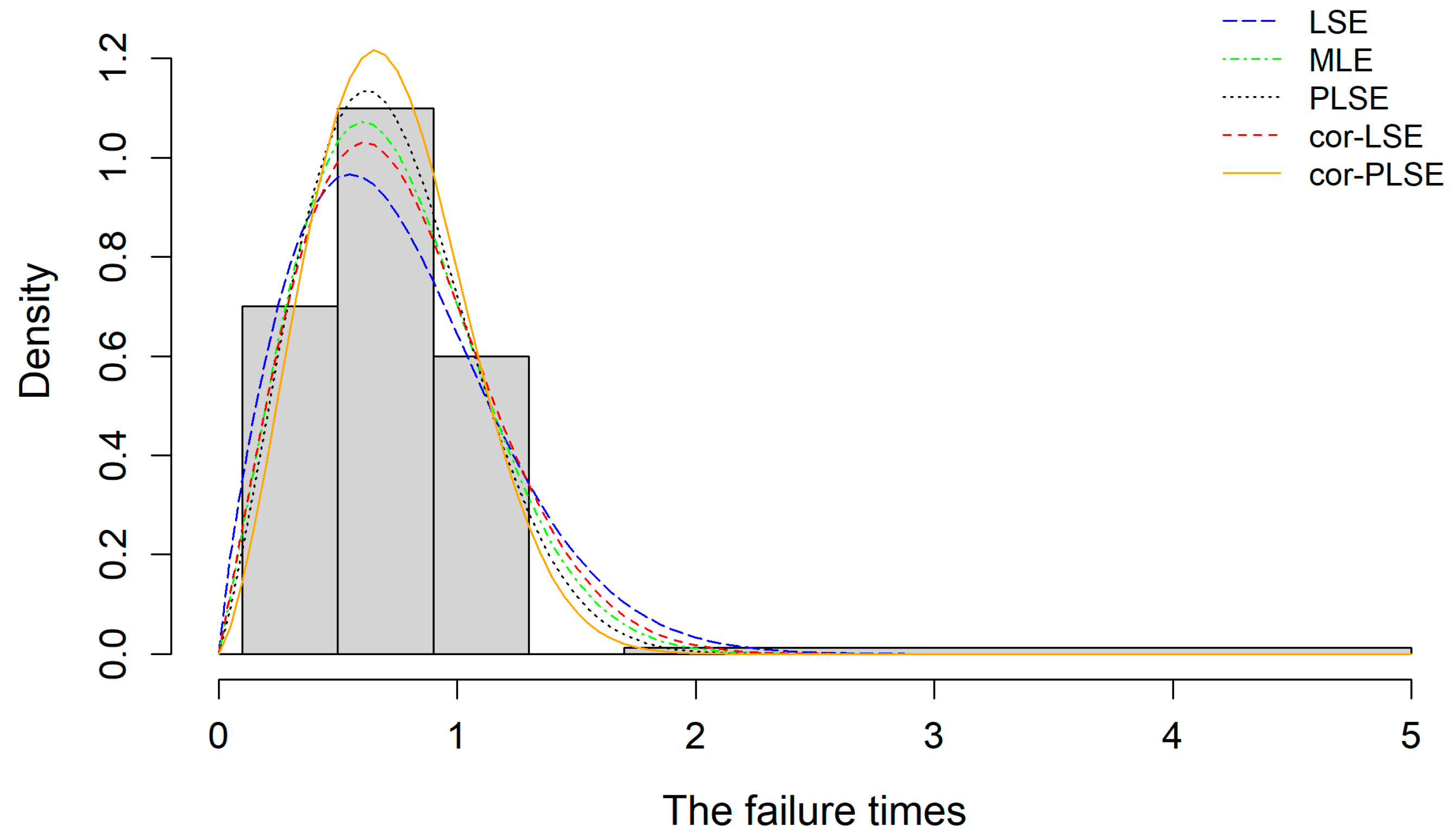
In addition, Figure 1 presents the fitted PDF for this dataset. The figure indicates that the performance of the estimation methods is generally similar, with the PLSE and bias-corrected PLSE providing fits that more accurately reflect the observed data. These observations are consistent with the conclusions reported in Section 4.

5.2. Example of New Drug-Induced Leukemia Remission Times

In this subsection, the proposed method is applied to a published dataset in [44] to illustrate the procedures. The dataset comprises remission times observed in leukemia patients treated with a new drug. The 22 remission times are as follows (in days):

47, 56, 58, 64, 77, 79, 89, 128, 131, 142, 144, 149, 163, 166, 175, 176, 184, 184, 188, 190, 191, 204.

As stated in [44], both the Kolmogorov-Smirnov test statistic and its corresponding p-value results indicate that the Weibull distribution provides an excellent fit for this data. We employ the Weibull distribution to model this dataset. To illustrate the application of the proposed method, we set $m=5$ and examine time points $T=50,$ 90, 130, 170, and 210. The complete sample is transformed into a Type I interval-censored dataset sample, with results presented in

Table 8. The Type I interval-censored data of remission times.

Time	(0, 50]	(50, 90]	(90, 130]	(130, 170]	(170, 210]	$(210, \mathbf{\infty }$]
Number	1	6	1	6	7	0

.

Based on the data in Table 8 and considering the LSL L = 0.05, the resulting estimates are as follows:

• MLE: ${\widehat{k}}_{\mathrm{M}LE}=$ 2.9180, ${\widehat{\lambda }}_{\mathrm{M}\mathrm{L}E}=$ 149.3540 and ${\widehat{C}}_{L,\mathrm{M}\mathrm{L}E}=$ 1.0000;
• LSE: ${\widehat{k}}_{LSE}=$ 2.4811, ${\widehat{\lambda }}_{LSE}=$ 145.6516 and ${\widehat{C}}_{L,LSE}=$ 0.9999;
• PLSE: ${\widehat{k}}_{PLSE}=$ 2.4811, ${\widehat{\lambda }}_{PLSE}=$ 145.6516, and ${\widehat{C}}_{L,PLSE}=$ 0.9999;
• Bias-corrected LSE: ${\widehat{k}}_{CLSE}=$ 2.5370, ${\widehat{\lambda }}_{CLSE}=$ 144.1888, and ${\widehat{C}}_{L,\mathrm{C}LSE}=$ 1.0000.
• Bias-corrected PLSE: ${\widehat{k}}_{CPLSE}=$ 2.6422, ${\widehat{\lambda }}_{CPLSE}=$ 144.9373, and ${\widehat{C}}_{L,\mathrm{C}\mathrm{P}LSE}=$ 1.0000.

For the results obtained from LSE, MLE, and PLSE, the MLE produces the largest estimates of $k$ and $\lambda$, as well as the highest value of ${\widehat{C}}_L$ (1.0000). In contrast, LSE and PLSE produce identical parameter estimates across all three metrics $k$, $\lambda$, and ${\widehat{C}}_L$, with their values of $k$ and $\lambda$ being lower than those from MLE, and their ${\widehat{C}}_L$ value slightly reduced to 0.9999. Following bias correction, the estimates of $k$ for both bias-corrected LSE and bias-corrected PLSE increase compared to their uncorrected counterparts (LSE and PLSE), whereas the estimates of $\lambda$ exhibit a slight decrease. Notably, the bias correction restores the value of ${\widehat{C}}_L$ back to 1.00 for both corrected methods, aligning it with the MLE result for this metric.

Based on ${\widehat{C}}_{L,MLE}$, the probability that the lifetime exceeds the lower specification limit can be estimated as $P\left(Y\ge L\right)=\exp \left\{{\widehat{C}}_{L,MLE}-1\right\}=$ 1.00. Similarly, using ${\widehat{C}}_{L,LSE}$, ${\widehat{C}}_{L,PLSE}$, ${\widehat{C}}_{L,\mathrm{C}LSE}$ and ${\widehat{C}}_{L,CPLSE}$, the corresponding probabilities $P(Y\ge LSL)$ are 0.9999, 0.9999, 1.0000, and 1.0000, respectively.

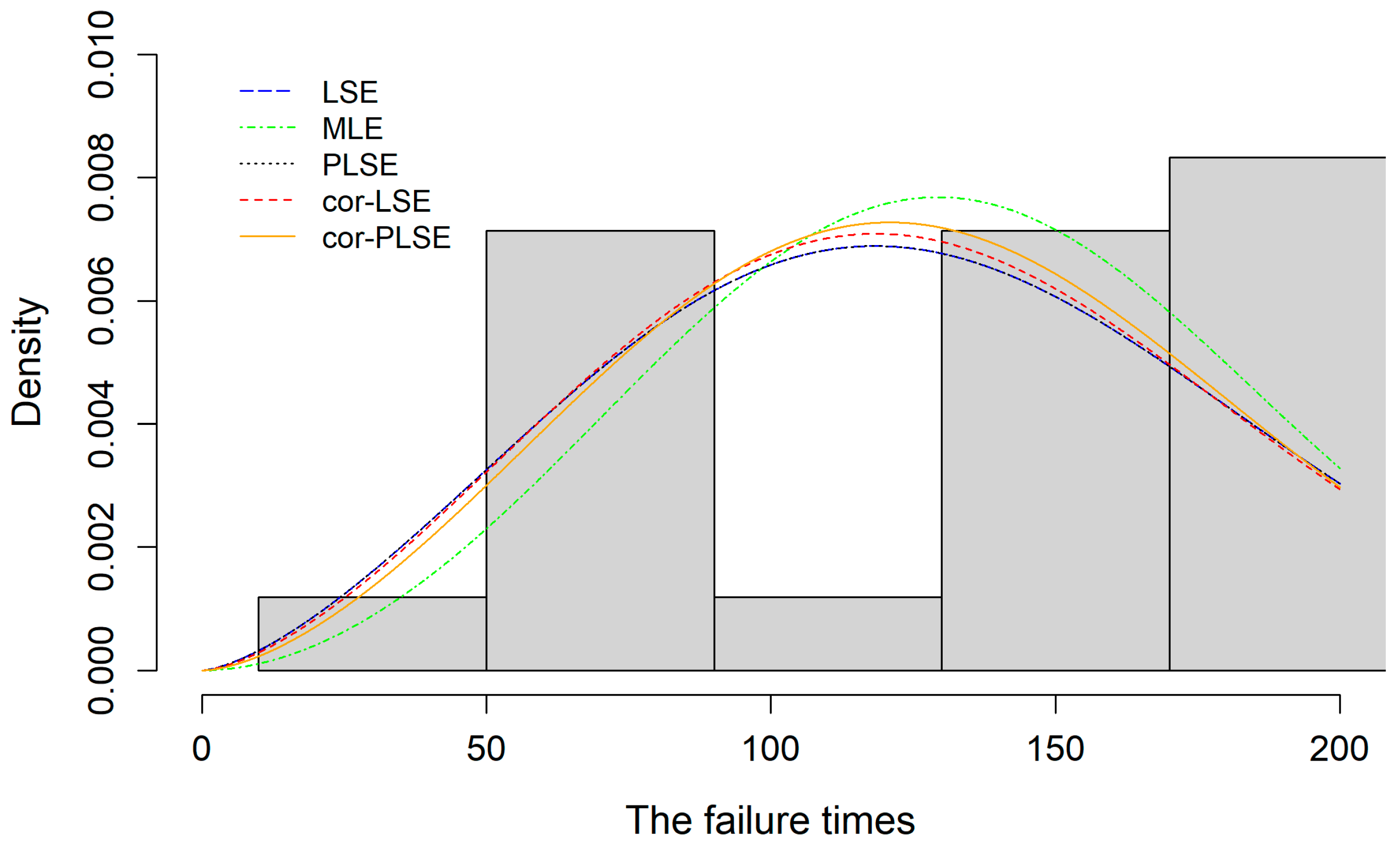
In addition, Figure 2 presents the fitted PDF for this dataset. The figure indicates that the performance of the estimation methods is generally similar, with the bias-corrected LSE and bias-corrected PLSE providing fits that more accurately reflect the observed data.

6. Conclusions

In this paper, we proposed four LSE methods to estimate the life performance index and the parameters of the Weibull distribution based on Type I interval-censored data. The proposed methods can provide closed-form solutions, offering clear advantages over widely used alternative approaches. The performance of the MLE and the proposed LSE methods was evaluated through simulation studies, using $A_b$ and MSE as comparison criteria. The results indicated that, without bias correction, the LSE and PLSE perform competitively. When bias correction is incorporated, the bias-corrected PLSE outperforms all other methods. It should be noted that an excessive number of intervals without observations may lead to an overestimation of the life performance index by the MLE or LSE methods, while PLSE will underestimate the life performance index. It is suggested not to use short time intervals for the proposed methods. Finally, two real data examples involving ball bearing failures and new drug-induced leukemia remission times were used to illustrate the proposed estimation methods. The analysis demonstrated that the LSE method provides reasonable and reliable parameter estimates.

A major challenge in parameter inference lies in obtaining the exact sampling distributions of the estimators. Alternative computational approaches may help alleviate difficulties arising from the unknown distributions of the model parameters. At the same time, the efficiency of the LSE decreases when the intervals are obtained without direct observations. In addition, in Equation (13), we use the “midpoint” of the interval to estimate the parameters, but this approach may lead to systematic bias in the estimators for biased distributions. Therefore, it is essential to explore strategies for improving the proposed methods and to investigate more robust estimation schemes based on enhanced experimental designs for the interval-censoring scheme. These issues remain open and will be addressed in future research.