Demand Forecast Investment by Overconfident Retailer in Supply Chains

Abstract

This paper investigates a supply chain setting in which a retailer exhibiting overconfidence invests in demand forecasting. Specifically, the retailer overestimates both the precision of the forecasting signal and the productivity of the investment. We analytically characterize the retailer’s investment behavior and show that overconfidence can lead to overinvestment in forecast accuracy. Beyond the investment decision itself, we examine how overconfidence influences the performance of both supply chain members and the system as a whole. When the retailer withholds forecast information from the supplier, overconfidence tends to harm both the retailer and the overall supply chain. However, under information-sharing arrangements, overconfidence can become beneficial—improving outcomes for the supplier and the system. Notably, when the retailer shares forecast with a sophisticated (strategically responsive) supplier, overconfidence may lead to a win–win outcome, where both parties gain from the retailer’s elevated investment in demand forecasting. These findings offer valuable insights into the conditions under which overconfidence shifts from being a liability to a strategic advantage, enriching our understanding of behavioral factors in supply chain decision-making.

1. Introduction

In today’s competitive business environment, companies increasingly invest in demand forecasting to enhance operational efficiency and strategic decision-making. By leveraging historical data, market trends, and relevant variables, demand forecasting predicts future customer demand. Accurate forecasts are critical for optimizing inventory management, minimizing stock-outs and overstocking, and ensuring timely production and delivery—key drivers of cost savings and customer satisfaction. Consequently, firms dedicate significant resources—time, capital, technology, and expertise—to improve forecast accuracy. This practice, termed demand forecast investment, encompasses acquiring advanced software, building a data analytics infrastructure, and training personnel to refine forecasting precision.

Retailers, positioned at the supply chain’s final link, are primary investors in demand forecasting. Faced with balancing supply and fluctuating consumer demand, accurate forecasts are vital for inventory planning, procurement, and coordination with upstream suppliers. As such, retailers often shoulder the costs of forecasting investments to mitigate risks of overstocking or stock-outs. Today, these investments are viewed as long-term strategic commitments central to maintaining competitive advantage.

Emerging behavioral research highlights cognitive biases influencing investment decisions, with overconfidence identified as a critical factor [1]. Overconfidence arises when individuals overestimate their knowledge, skills, or ability to generate exceptional returns [2]. As one of the most pervasive and robust cognitive biases [3], it has been documented in economics [4], finance [5], and consumer behavior [6].

In demand forecasting, overconfidence manifests when planners overestimate their predictive capabilities [7,8]. Surveys reveal that executives frequently exhibit unwarranted confidence in their forecasting precision, leading to suboptimal investments https://tools.north-find.com/bias-tool, accessed on 1 March 2025. For example, managers launching new products often inflate expectations of forecast accuracy [9]. Overconfidence also drives excess investment—allocating excessive resources despite uncertain returns [10,11]. Anecdotal evidence aligns with this: U.S. retailers spend billions annually on forecasting tools, yet only 60% rate their forecasts positively, while 34% report poor investment outcomes https://progressivegrocer.com/strengthening-retail-supply-chain-survey-50-leading-us-retailers, accessed on 1 March 2025.

This overconfidence can ripple through supply chains. Retailers often share forecasts with suppliers [12], and if investments are unobservable, suppliers may misinterpret forecast precision, compounding inefficiencies. However, sophisticated suppliers who account for forecast accuracy can mitigate these effects. Thus, overconfidence not only distorts retailer decisions but also impacts broader supply chain dynamics.

Against this backdrop, we analyze how retailer overconfidence in demand forecast investment affects supply chain performance. We model a retailer investing in forecast precision while overestimating both her signal’s accuracy and investment efficacy. Our study addresses the following:

• How does overconfidence influence retailers’ demand forecast investment levels?
• Is overconfidence universally detrimental to supply chain members and system- wide performance?
• Does information sharing amplify or alleviate overconfidence’s effects?

We begin our analysis by considering the case of no information sharing, where the retailer keeps the forecast confidential. As a validation for our model, we analytically show that the widely observed excess investment effect also exists in our context—that is, the overconfident retailer invests more than the unbiased retailer. However, overconfidence may also hinder retailers’ investments in demand forecasting, especially when the retailer subjectively perceives that the forecasting information is sufficiently accurate. Our analysis reveals that greater overconfidence always leads to lower retailer performance. This is because overconfidence distorts investment decisions, causing the equilibrium investment level to deviate from the optimal, thereby negatively affecting both the retailer and the entire supply chain.

We extend our analysis to the case where the retailer truthfully shares the forecast with the supplier. We show that, like in the no-information-sharing scenario, the excess investment effect persists in this setting. Moreover, the overconfident retailer adopts the same decision policy as the unbiased retailer—that is, lowering investment in demand forecasting when information is shared. Although overconfidence consistently hurts the retailer, this bias can actually be a positive force for the supplier and the entire system—that is, as overconfidence increases, both the supplier’s and the system’s overall performance improves.

To put this into perspective, we examine the first-best benchmark in which an unbiased planner coordinates the retailer and supplier to maximize aggregate profits. Without such coordination, the supplier and the retailer would make decisions independently, leading to underinvestment in forecasting and the system being worse off. However, if a biased retailer replaced the unbiased one, the system may perform better, depending on the level of overconfidence. Intuitively, overconfidence can increase forecasting investment, partially offsetting the underinvestment caused by decentralization. As a result, the entire system can benefit from the retailer’s overconfidence.

Finally, we conduct additional robustness tests with two model variants: observable investment and a sophisticated supplier. Our results suggest that the main finding—that both the supplier and the entire supply chain can benefit from overconfidence under information sharing—holds in these extensions, although the analysis becomes rather involved. More interestingly, in the case of sophisticated supplier, a win–win outcome can prevail in which both the retailer and the supplier benefit from overconfidence. For insight, a more severe overconfidence has two opposing effects on the retailer. The first effect is that overconfidence distorts the retailer’s investment and retail pricing decisions, thereby harming the retailer. The second effect is that the shared forecast with increased precision encourages the sophisticated supplier to set a wholesale price that mitigates the retailer’s pricing distortion, thus benefiting the retailer. If the second effect outweighs the first, the retailer may benefit from higher overconfidence.

The rest of this paper is organized as follows. The related literature is reviewed in Section 2. In what follows, we introduce the demand forecast investments in Section 3 and overconfidence in Section 4. We later extend our analysis to the case with information sharing in Section 5. Section 6 conducts a robustness check of our main findings. We conclude our research in Section 7.

2. Literature Review

This study is related to two streams of research: (i) bias in demand forecasting and (ii) information sharing.

2.1. Bias in Demand Forecasting

Demand forecasting, a key aspect of operations management, has been widely studied over the past decade, e.g., [13,14,15,16,17,18]. Recent research has explored the implication of advanced techniques in forecasting, such as artificial intelligence [19] and machine learning [20]. Despite these advancements, which promise automated, data-driven predictions, the practical implementation of demand forecasting still relies heavily on human judgment [21]. A 2015 survey revealed that only 29% of forecasting organizations exclusively used statistical methods; most employed a hybrid approach, combining statistical forecasts with human judgment [22]. This human involvement introduces various biases into the forecasting process, as shown in the literature, e.g., [15,23,24,25,26,27,28,29].

This research, focusing on various behavioral biases that can affect the forecasting process in different contexts, can be divided into two categories: “point forecasting” and “forecasting a distribution”. Point forecasting involves providing a single estimate of future demand, with biases such as anchoring [30] and system neglect [23] being well documented. More recent studies focus on forecasting a distribution, which provides a detailed view of the underlying probability distribution. A key bias in this category is overprecision, a form of overconfidence where individuals underestimate uncertainty or narrowly define the distribution (there are three types of overconfidence: overprecision, overestimation, and overplacement; see [31] for details). For example, ref. [32] shows that overprecision can explain the pull-to-center effect in the newsvendor model. Ref. [9] finds that managers launching new products often overlook forecast uncertainty, leading to overconfidence and underestimation of errors.

As opposed to overprecision, the particular form of overconfidence explored in this paper involves the overestimation of a retailer’s ability to make effective demand forecast investments. Specifically, we develop a model in which the overconfident retailer not only perceives excessive precision in her forecasts but also overestimates the effectiveness of her forecasting efforts. As a result, this work contributes to the field of behavioral operations management by examining the theoretical impact of overconfidence in demand forecast investments.

2.2. Information Sharing

Our work also relates to the extensive literature on information sharing between downstream firms (retailers) and upstream firms (manufacturers or suppliers) in two-tier supply chains; see [33,34,35,36] and the references therein. Recent research in this area focuses on two main streams. The first examines the impact of information sharing on supply chain efficiency. For example, ref. [37] studied the benefits of sharing component quality information between suppliers and assemblers. Ref. [38] explored how platform information sharing influences third-party suppliers and offline retailers, finding that it increases the likelihood of adopting the agency model. Ref. [39] investigated the value of information sharing and acquisition by manufacturers in the context of manufacturer encroachment.

The second stream examines how operations and marketing strategies influence information sharing. Ref. [40] showed that encroachment and information sharing are complementary strategies, emphasizing the need for managers to consider their interdependent effects. Similarly, ref. [41] introduced a wholesale pricing mechanism that facilitates information sharing between a weaker retailer and a dominant manufacturer, benefiting both parties. Ref. [42] explored how information sharing between a retail platform and a manufacturer affects product quality and supply chain dynamics, focusing on the role of quality signals and product reviews. Ref. [43] demonstrated that the flexibility of a manufacturer’s product line could incentivize a retailer to share private demand information, challenging traditional views on retailer–manufacturer information asymmetry.

Most information-sharing literature assumes rational decision-makers, as noted above. In contrast, we examine information sharing between a supplier and a retailer exhibiting overconfidence bias in investment decisions. This leads to two key contributions. First, overconfidence can benefit both the supplier and the entire supply chain. Second, a win–win outcome can emerge where both the retailer and the supplier benefit from overconfidence when the retailer shares forecasts with a sophisticated supplier. Although prior research has highlighted the benefits of information sharing, our study offers a more nuanced perspective by exploring its potential to mitigate the negative effects of overconfidence.

3. Model Setup

Consider a single-period supply chain comprising a supplier (he) and a retailer (she). The supplier manufactures a product and distributes it exclusively through the retailer. The sequence of events unfolds as follows: First, the supplier determines the wholesale price per unit, denoted as w. Upon observing w, the retailer subsequently sets the retail price p to customers before market demand is realized. In this paper, we adopt a linear demand function with additive uncertainty primarily for its analytical tractability and interpretability, which allows us to isolate and clearly examine the behavioral impact of overconfidence on forecast investment decisions. Specifically, our demand function is

$$D=a+\theta -p,$$

(1)

where $a>0$ denotes the market potential. To capture the uncertainty of demand, we assume that $\theta$ is a random variable with zero mean and variance ${\sigma }^2:=Var\left[\theta \right]$. Suppose $a^2$ is large relative to ${\sigma }^2$, to ensure non-negative demand. Without loss of generality, we assume that the production cost for the supplier is zero.

While this linear form is widely used in the literature on behavioral operations and supply chain modeling, e.g., [34], we recognize that multiplicative demand functions are also common and often capture demand heteroscedasticity. However, incorporating multiplicative uncertainty introduces endogenous variance and additional complexity into the analysis of overconfidence, which may obscure the primary behavioral mechanisms we aim to highlight.

The retailer may invest in demand forecasting investment—long-term strategic actions that precede short-term pricing and sales decisions. These investments include initiatives such as hiring a business intelligence team, procuring forecasting software, or contracting third-party agencies with varying service-level agreements. Upon investing, the retailer obtains a private signal s about the uncertain demand parameter $\theta$. The precision of s, denoted $v\left(\lambda \right)$, depends on the investment level $\lambda$. The higher the $v\left(\lambda \right)$ value, the greater the signal accuracy: $v\left(\lambda \right)=0$ implies a useless signal, while $v\left(\lambda \right)\to \infty$ represents perfect foresight.

We model the precision function $v\left(\lambda \right)$ as increasing and concave in $\lambda$, with $v\left(0\right)=0$. Formally, $v^{\prime }\left(\lambda \right)>0$ and $v^{″}\left(\lambda \right)\le 0$. This reflects diminishing marginal returns to investment—each additional unit of investment improves precision but at a decreasing rate. Following established literature, e.g., [34,44,45,46], we adopt an unbiased signal structure with affine conditional expectations. Specifically, $E\left[s\right|\theta ]=\theta$ and $E\left[\theta \right|s]={\displaystyle \frac{v·s}{1+v}}$. This framework generalizes to accommodate diverse demand distributions while maintaining analytical tractability [34].

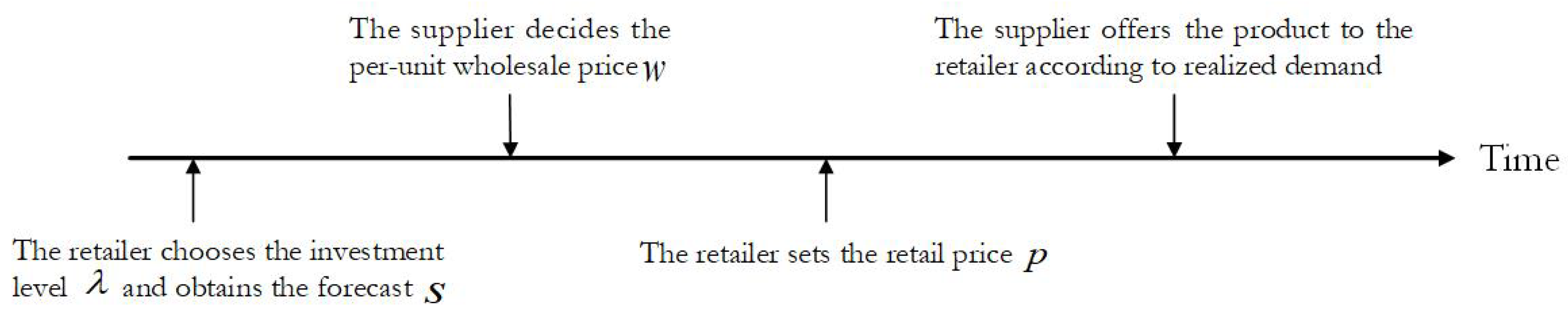
The sequence of events unfolds as follows: (1) The retailer selects an investment level $\lambda$ to obtain a private demand signal s, with accuracy $v\left(\lambda \right)$; (2) the supplier determines the per-unit wholesale price w for transferring the product to the retailer. (3) Conditional on w and the acquired signal s, the retailer sets the consumer-facing retail price p; (4) the selling season commences. The retailer orders inventory from the supplier based on realized demand, and transfer payments are settled. See Figure 1 for a graphic depiction of the game and model variables. We assume the retailer does not disclose her private signal to the supplier. This assumption is relaxed in Section 5.

We solve this game by backward induction as follows. In the third stage, given the observed signal s with accuracy $v\left(\lambda \right)$ and the wholesale price w, the retailer determines the retail price p to maximize her profit:

$$\underset{p}{max}{\pi }_r(p,w,\lambda ):=(p-w)\left[a+{\displaystyle \frac{v\left(\lambda \right)s}{1+v\left(\lambda \right)}}-p\right]-\lambda .$$

Thus, the equilibrium retail price is

$$p^{\ast }(\lambda ,w)={\displaystyle \frac{1}{2}}\left(a+{\displaystyle \frac{v\left(\lambda \right)s}{1+v\left(\lambda \right)}}+w\right).$$

(2)

Due to the absence of information-sharing activity, in the second stage, the supplier holds his prior belief about $\theta$ and thus anticipates that the retail price is $(a+w)/2$. In other words, the supplier’s problem in this stage is equivalent to

$$\underset{w}{max}\left\{w\left(a-{\displaystyle \frac{a+w}{2}}\right)\right\},$$

which leads to the optimal wholesale price being $w^{\ast }=a/2$. By replacing equilibrium actions with expressions for retailer profit and then taking expectations conditional on s, the retailer’s problem in the first stage is equivalent to setting the investment level $\lambda$ to maximize the expected profit

$$E\left[{\pi }_r(p^{\ast },w^{\ast },\lambda )\right]={\displaystyle \frac{a^2}{16}}+{\displaystyle \frac{v\left(\lambda \right){\sigma }^2}{4[1+v(\lambda \left)\right]}}-\lambda .$$

(3)

Lemma 1 below describes the equilibrium investment level.

Lemma 1.

The (unbiased) retailer’s optimal investment level ${\lambda }^{\ast }$ is characterized by

$${\displaystyle \frac{{\sigma }^2{v}^{\prime }\left(\lambda \right)}{4{(1+v\left(\lambda \right))}^2}}=1$$

if $v^{\prime }\left(0\right){\sigma }^2/4>1$. Otherwise, ${\lambda }^{\ast }=0$.

Lemma 1 suggests that when the marginal cost exceeds the expected profit at the zero investment level, i.e., $v^{\prime }\left(0\right){\sigma }^2/4\le 1$, it is unprofitable for the retailer to invest in forecasting.

We formalize overconfidence in demand forecast investment by modeling the retailer’s biased perception of signal precision. Drawing on prior work, e.g., [47,48,49], we define overconfidence as a cognitive distortion where the retailer subjectively believes the precision of her demand signal to be

$$\widehat{v}(\alpha ,\lambda ):=\alpha ·v\left(\lambda \right)$$

(4)

for a given investment level $\lambda$, despite the true precision remaining $v\left(\lambda \right)$. Here, $\alpha \ge 1$ quantifies the degree of overconfidence. The rational benchmark corresponds to $\alpha =1$, while $\alpha >1$ reflects an overconfident retailer who overestimates both the precision of her signal ($\widehat{v}>v\left(\lambda \right)$) and the marginal returns on her investment.

Within this framework, subjective precision and the marginal precision per unit investment are increasing in overconfidence—that is,

$${\displaystyle \frac{\partial \widehat{v}}{\partial \alpha }}>0,{\displaystyle \frac{{\partial }^2\widehat{v}}{\partial \lambda \partial \alpha }}>0.$$

Therefore, overconfidence also distorts the retailer’s belief in the marginal value of additional investment, leading to excessive resource allocation. This framework aligns with empirical observations that overconfident entrepreneurs overinvest in forecasting efforts, driven by unwarranted faith in their predictive capabilities. Notably, we assume the retailer is unaware of her bias; she operates under the belief that $\widehat{v}(\alpha ,\lambda )$ reflects true precision, without knowledge of $\alpha$. Following [50], we model the supplier–retailer game under the premise that each agent acts rationally based on their beliefs about the other’s behavior. The supplier sets wholesale prices anticipating the retailer’s biased investment and pricing decisions, while the retailer optimizes her choices under-inflated confidence in her forecast accuracy.

4. Equilibrium Analysis

In this section, we analyze the equilibrium for demand forecast investment and examine the comparative statics of investment.

In the third stage, given the observed signal s with the subjective accuracy $\widehat{v}(\alpha ,\lambda )$ and the wholesale price w, the biased retailer behaves as if

$$\underset{p}{max}\left\{(p-w)\left[a+{\displaystyle \frac{\widehat{v}(\alpha ,\lambda )s}{1+\widehat{v}(\alpha ,\lambda )}}-p\right]-\lambda \right\}.$$

By solving this, the biased retailer sets the retail price as

$$\widehat{p}(\lambda ,w):={\displaystyle \frac{1}{2}}\left(a+{\displaystyle \frac{\widehat{v}(\alpha ,\lambda )s}{1+\widehat{v}(\alpha ,\lambda )}}+w\right).$$

(5)

Since the forecast cannot be disclosed to the supplier, the supplier maintains his prior belief in market potential. Thus, the supplier’s pricing policies accordingly follow the standard theory—that is, $w^{\ast }=a/2$. With a parameter $\alpha$, the retailer behaves as if she were enjoying a profit of (3), except with $\widehat{v}(\alpha ,\lambda )$ in place of $v\left(\lambda \right)$. Proposition 1 characterizes the biased retailer’s equilibrium investment $\widehat{\lambda }\left(\alpha \right)$.

Proposition 1.

For a given overconfidence parameter α,

(a) The (biased) equilibrium investment level $\widehat{\lambda }\left(\alpha \right)$ is uniquely determined by

$${\displaystyle \frac{{\sigma }^2\alpha v^{\prime }\left(\lambda \right)}{4{(1+\alpha v\left(\lambda \right))}^2}}=1$$

if $\alpha v^{\prime }\left(0\right){\sigma }^2/4>1$ and otherwise $\widehat{\lambda }\left(\alpha \right)=0$.

(b) $\widehat{\lambda }\left(\alpha \right)$ is increasing in α, i.e., $\partial \widehat{\lambda }\left(\alpha \right)/\partial \alpha >0$, if and only if $\alpha v\left(\widehat{\lambda }\right)<1$.

Proposition 1a indicates that when the unbiased retailer has no incentive to invest in demand forecasting ($v^{\prime }\left(0\right){\sigma }^2/4\le 1$), the biased retailer ($\alpha >1$) would invest in demand forecasting if the subjective marginal return is higher than the margin cost, i.e., $\alpha v^{\prime }\left(0\right){\sigma }^2/4>1$. Intuitively, overconfidence causes the retailer to overestimate her ability to profit from forecasting activity, thus inducing her to invest in demand forecasting.

Proposition 1b shows that as the overconfidence level increases, the investment level in forecasting can be higher than before. For an illustration, we assume that the actual precision function is

$$v\left(\lambda \right):=\kappa ·{\lambda }^{\beta },$$

(6)

where $\kappa >0$ is the operational efficiency of forecasting investment. As $\kappa$ increases, the retailer can invest to forecast demand more efficiently. Let $0<\beta \le 1$ to ensure incrementality and concavity. Note that (6) has been used in the operations literature to derive insights, e.g., [51]. Let ${\sigma }^2=20$ and $\kappa =0.4$. These parameters were selected to illustrate a representative case where the marginal return of forecast investment is meaningful. This choice enables us to clearly demonstrate the behavioral and performance implications of overconfidence while ensuring that forecast investment remains positive across all levels of overconfidence. Figure 2 illustrates how the biased investment level ($\widehat{\lambda }$) changes with respect to the overconfidence level ($\alpha$) for different values of $\beta$. As per this figure, when overconfidence is relatively low, the retailer invests more in forecasting as she becomes more biased. However, when overconfidence is relatively high, the investment level decreases with $\alpha$.

For insight, overconfidence motivates the retailer to invest more in forecasting when the perceived precision of the signal is low ($\alpha v\left(\widehat{\lambda }\right)<1$). This occurs because the overconfident retailer perceives higher productivity from her investment. As a result, overconfidence leads to greater investment, especially when the retailer believes the forecast is insufficiently accurate. However, when the perceived accuracy is high ($\alpha v\left(\widehat{\lambda }\right)\ge 1$), the biased investment level $\widehat{\lambda }$ decreases with higher overconfidence, as the retailer feels less need to invest further when the forecast appears accurate enough.

After obtaining the biased investment level $\widehat{\lambda }\left(\alpha \right)$, we evaluate the impacts of overconfidence on the retailer’s profit. While the retailer makes decisions with the subjective precision function, the actual precision function still counts in the retailer’s resulting profit function. In other words, the resulting expected profit of the biased retailer is given by

$${\widehat{\pi }}_r^{\ast }:=E\left[{\pi }_r(\widehat{p},w^{\ast },\widehat{\lambda })\right]=E\left[(\widehat{p}-w^{\ast })\left(a+{\displaystyle \frac{v\left(\widehat{\lambda }\right)s}{1+v\left(\widehat{\lambda }\right)}}-\widehat{p}\right)-\widehat{\lambda }\right].$$

To obtain more insights, we consider a linear function, i.e., $v\left(\lambda \right)=\kappa ·\lambda$, which allows for a simplified equilibrium analysis that aids in understanding the basic relationships and dynamics. In fact, the linear relationship between forecast accuracy and investment cost is commonly used in various forecasting and operational management studies (see, e.g., [52,53]) (note that [53] denotes the cost function for demand forecasting by C: to achieve a forecast accuracy v, the retailer must invest $C\left(v\right)$. In other words, the independent variable in this function is forecast accuracy v. In contrast, our paper considers a forecast accuracy function v based on the investment level $\lambda$: when the retailer invests $\lambda$, she obtains a forecast with accuracy $v\left(\lambda \right)$. In this sense, the investment cost function $C\left(v\right)$ and the forecast accuracy function $v\left(\lambda \right)$ are inverses of each other. Ref. [53] analyzed the comparative statics for the linear demand forecast investment cost case to obtain more insights. Essentially, the linear investment cost case is equivalent to the linear forecast accuracy case. Our reference to this work is intended to highlight the linear relationship between forecast accuracy and investment cost.).

Proposition 2.

For linear precision functions, i.e., $v\left(\lambda \right)=\kappa ·\lambda$, the biased retailer’s expected profit ${\widehat{\pi }}_r^{\ast }$ decreases with the overconfidence level α.

Proposition 2 indicates that the retailer suffers from overconfidence, which aligns with our intuitive expectation that cognitive bias leads to self-detriment. Intuitively speaking, the biased retailer tends to overinvest or underinvest compared to the unbiased counterpart, ultimately being worse off. Specifically, overinvestment driven by biased perceptions can increase operational costs without yielding proportional benefits. On the other hand, underinvestment prevents the retailer from obtaining sufficiently accurate forecasting information to manage the risks arising from demand uncertainty.

Next, we resort to numerical experiments to seek the robustness of Proposition 2. By utilizing (6), we plot the retailer’s performance in Figure 3 for different values of $\beta$. We also denote ${\sigma }^2=20$ and $\kappa =0.4$ to ensure the positive realizations of the biased investment level, i.e., $\widehat{\lambda }\left(\alpha \right)>0$ for any $\alpha >1$. As per this figure, for non-linear accuracy functions ($\beta <1$), the retailer’s profit also decreases as overconfidence level $\alpha$ increases. This indicates that the retailer always suffers from overconfidence bias.

Note that when the retailer keeps the forecast confidential to the supplier, overconfidence does not directly affect the supplier’s performance. As a result, overconfidence consistently harms both the retailer and the entire system. However, this negative effect may be mitigated if the retailer voluntarily shares the forecast with the supplier, as discussed in the following sections.

5. Information Sharing

We first introduce the information-sharing model without overconfidence. Following the typical framework in information sharing between supply chain members, e.g., [12], the retailer would honestly disclose the forecast to the monopoly supplier. The assumption of truthful sharing would be valid, especially when the retailer engages the monopolistic supplier and values its reputation to maintain long-term cooperation with the supplier. Thus, the supplier may set the wholesale price w based on the shared signal s. This section assumes that the retailer’s actual investment level is unobservable. We relax this assumption in Section 6.1.

We next characterize the equilibrium outcome for this model. Given the observed signal s and the wholesale price w, the equilibrium retail price in this setting is also given by $p^{\ast }$, as defined in (2). After receiving the shared signal s with the claimed precision $v\left(\lambda \right)$ and anticipating that the equilibrium retail price is $p^{\ast }$, the optimization problem of the supplier in the second stage is defined as

$$\underset{w}{max}{\pi }_s(p^{\ast },w,\lambda ):=w\left(a+{\displaystyle \frac{v\left(\lambda \right)s}{1+v\left(\lambda \right)}}-p^{\ast }\right).$$

This leads to the equilibrium wholesale price being

$$w^o:={\displaystyle \frac{1}{2}}\left(a+{\displaystyle \frac{v\left(\lambda \right)s}{1+v\left(\lambda \right)}}\right).$$

(7)

By replacing equilibrium actions with expressions for retailer profit and then taking expectations conditional on s, the retailer’s problem in the first stage is equivalent to maximizing her expected profit

$$\underset{\lambda }{max}E\left[{\pi }_r(p^{\ast },w^o,\lambda )\right]={\displaystyle \frac{a^2}{16}}+{\displaystyle \frac{{\sigma }^{2}v\left(\lambda \right)}{16[1+v(\lambda \left)\right]}}-\lambda .$$

(8)

The comparison between the second term of (3) and (8) implies that information sharing reduces the value forecast generated by the retailer. Solving (8), the (unbiased) equilibrium investment level ${\lambda }^o$ is uniquely determined by

$${\displaystyle \frac{{\sigma }^2{v}^{\prime }\left(\lambda \right)}{16{[1+v\left(\lambda \right)]}^2}}=1$$

if ${\sigma }^2{v}^{\prime }\left(0\right)/16>1$; otherwise, ${\lambda }^o=0$.

Next, we consider the biased retailer’s investment decision in the context of information sharing. In the third stage, the biased retailer sets the retail price as $\widehat{p}(\lambda ,w)$, as defined in (5). In this setting, the retailer discloses the signal s to the supplier and claims the precision is $\widehat{v}(\alpha ,\lambda )$. Since the supplier can not observe the actual investment level $\lambda$, the supplier believes the precision of the signal is $\widehat{v}(\alpha ,\lambda )$ rather than the actual precision $v\left(\lambda \right)$. Therefore, the supplier behaves as if

$$\underset{w}{max}\left\{w\left(a+{\displaystyle \frac{\widehat{v}(\alpha ,\lambda )s}{1+\widehat{v}(\alpha ,\lambda )}}-\widehat{p}\right)\right\}.$$

Thus, the equilibrium wholesale price is given by

$${\widehat{w}}^o:={\displaystyle \frac{a}{2}}+{\displaystyle \frac{\widehat{v}(\alpha ,\lambda )s}{2(1+\widehat{v}(\alpha ,\lambda ))}}.$$

(9)

For a retailer with an overconfidence parameter $\alpha$, the retailer behaves as if she were enjoying a profit of (8), except with $\widehat{v}(\alpha ,\lambda )$ in place of $v\left(\lambda \right)$.

Proposition 3.

When the biased retailer shares the forecast with the supplier,

(a) the biased investment level ${\widehat{\lambda }}^o$ uniquely satisfies

$${\displaystyle \frac{{\sigma }^2\alpha v^{\prime }\left(\lambda \right)}{16{[1+\alpha v\left(\lambda \right)]}^2}}=1$$

if ${\sigma }^2\alpha v^{\prime }\left(0\right)/16>1$. Otherwise, ${\widehat{\lambda }}^o=0$.

(b) ${\widehat{\lambda }}^o$ is increasing in α, i.e., $\partial {\widehat{\lambda }}^o\left(\alpha \right)/\partial \alpha >0$, if and only if $\alpha v\left(\widehat{{\lambda }^o}\right)<1$.

(c) The biased retailer with information sharing sets a lower investment level than without—that is, ${\widehat{\lambda }}^o\left(\alpha \right)\le \widehat{\lambda }\left(\alpha \right)$ for a given α.

Propositions 3a,b extend the standard structural properties established in Proposition 1 to the information-sharing context. While the retailer’s forecasting investment strategy may change with information sharing, the fundamental behavioral dynamics remain the same. Furthermore, Proposition 3c shows that information sharing reduces forecasting investment, as it diminishes the perceived value of the forecast, thus prompting the retailer to invest less.

Given the biased investment level ${\widehat{\lambda }}^o$, the retailer’s resulting expected profit is

$${\widehat{\pi }}_r^o=E\left[{\pi }_r(\widehat{p},{\widehat{w}}^o,{\widehat{\lambda }}^o)\right]=E\left[(\widehat{p}-{\widehat{w}}^o)\left(a+{\displaystyle \frac{v\left({\widehat{\lambda }}^o\right)·s}{1+v\left({\widehat{\lambda }}^o\right)}}-\widehat{p}\right)-{\widehat{\lambda }}^o\right].$$

Accordingly, the ensuing supplier’s equilibrium profit is

$${\widehat{\pi }}_s^o=E\left[{\pi }_s(\widehat{p},{\widehat{w}}^o,{\widehat{\lambda }}^o)\right]=E\left[{\widehat{w}}^o\left(a+{\displaystyle \frac{v\left({\widehat{\lambda }}^o\right)·s}{1+v\left({\widehat{\lambda }}^o\right)}}-\widehat{p}\right)\right].$$

Next, we explore how overconfidence affects the performance of supply chain members.

Proposition 4.

Suppose $v\left(\lambda \right)=\kappa ·\lambda$. We obtain the following aspects:

(a) The retailer’s equilibrium profit ${\widehat{\pi }}_r^o$ always decreases in overconfidence level α.

(b) Within a certain range of overconfidence levels, the supplier’s equilibrium profit ${\widehat{\pi }}_s^o$ increases as the overconfidence level α rises.

Proposition 4a indicates that overconfidence bias always hurts the retailer in the context of information sharing. For illustration, we plot ${\widehat{\pi }}_r^o$ in Figure 4 by specifying the precision function as (6). From Proposition 3, we let ${\sigma }^2=50$ and $\kappa =0.4$ to ensure ${\widehat{\lambda }}^o>0$ for any $\alpha >1$. As per this figure, the biased retailer’s profit decreases with $\alpha$ for $\beta \in \{0.2,0.5,0.8,1\}$. 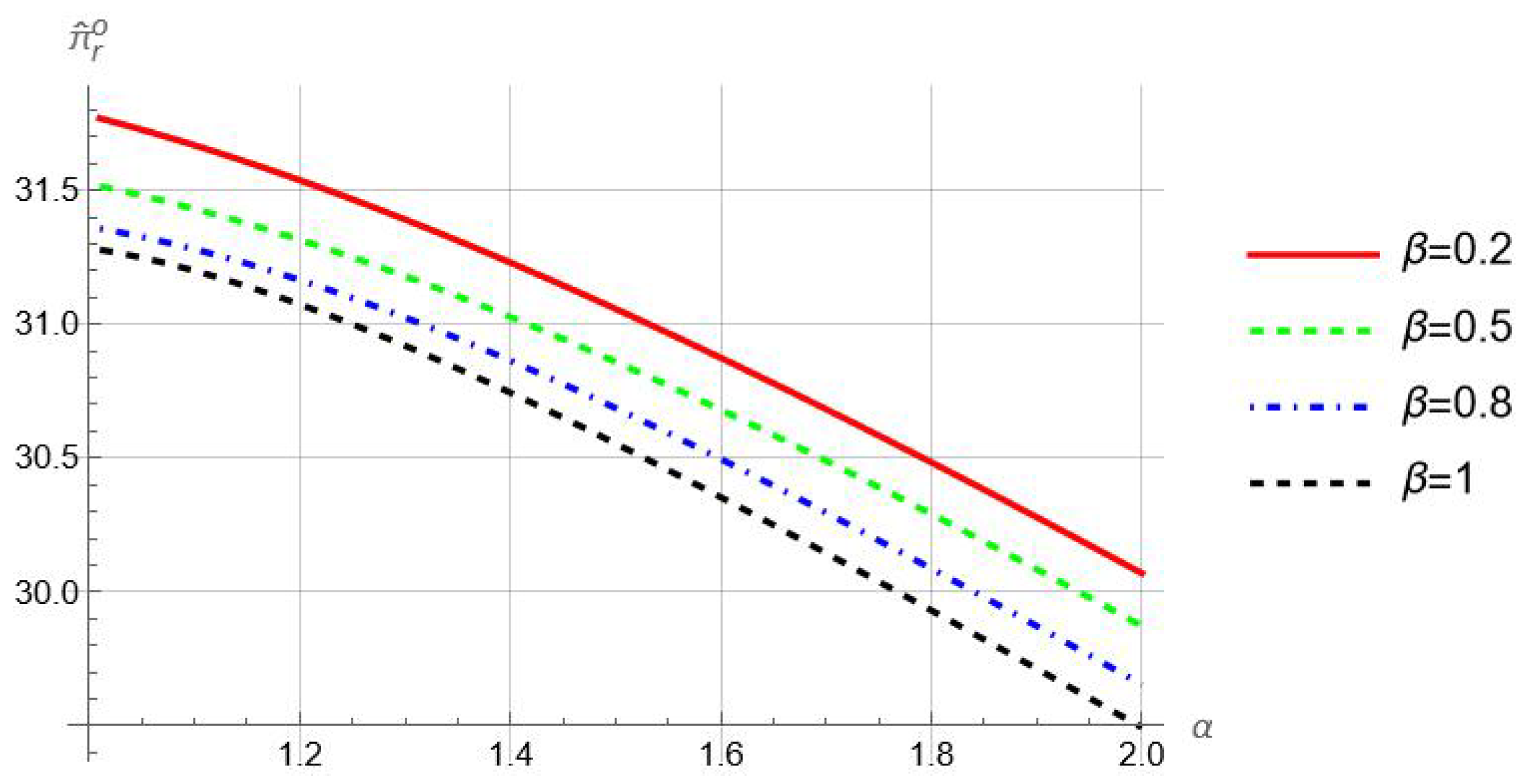Intuitively, more severe overconfidence exacerbates the distortion in investing behaviors from optimality, thus hurting the retailer. This is consistent with the case without information sharing, where overconfidence harms the retailer.

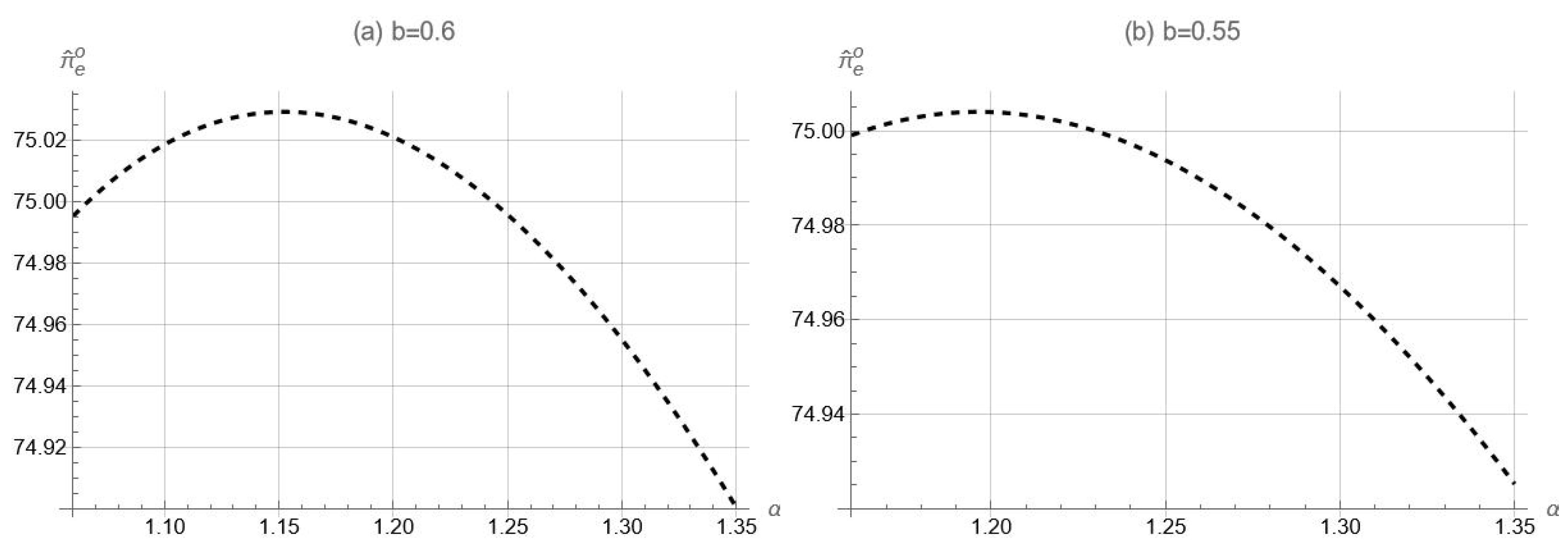
Proposition 4b indicates that under information sharing, retailer overconfidence can potentially benefit the supplier. To illustrate this, we plot how ${\widehat{\pi }}_s^o$ changes with respect to the parameter $\alpha$ in Figure 5 by specifying $v\left(\lambda \right)=\kappa ·{\lambda }^{\beta }$. Let ${\sigma }^2=42.5$ and $\kappa =0.4$ to ensure that ${\widehat{\lambda }}^o>0$ for any $\alpha$. For $\beta \in \{0.85,0.9,0.95\}$, Figure 5 indicates that our key result—the supplier can benefit from retailer overconfidence—continuously holds for the non-linear accuracy function. Furthermore, Figure 5 demonstrates that the range of overconfidence levels such that overconfidence benefits the supplier becomes larger as the value of $\beta$ increases. In fact, when adjusting the values of other parameters in (6), such as reducing $\kappa$ or using alternative accuracy functions, the impact of overconfidence is even more significant. This implies that our results are not only restricted to very low overconfidence. See Appendix B for details.

For insight, retailer overconfidence affects the supplier’s performance in two opposing ways. The first (direct) impact is negative—overconfidence leads the supplier to set irrational wholesale prices based on the forecast with “wrong” accuracy, as shown in (9). The second (indirect) impact, however, can be positive—higher overconfidence may improve forecast precision (Proposition 3b), enabling the supplier to make better decisions. The overall effect on supplier performance depends on the balance between these forces. When overconfidence is low, the positive impact of improved forecast accuracy generally outweighs the negative effect. Proposition 4b reveals an interesting dynamic: overconfidence in retailers can unintentionally benefit suppliers within an information-sharing framework. By promoting information sharing, suppliers gain access to more accurate demand forecasts, helping them optimize production schedules to align with anticipated demand.

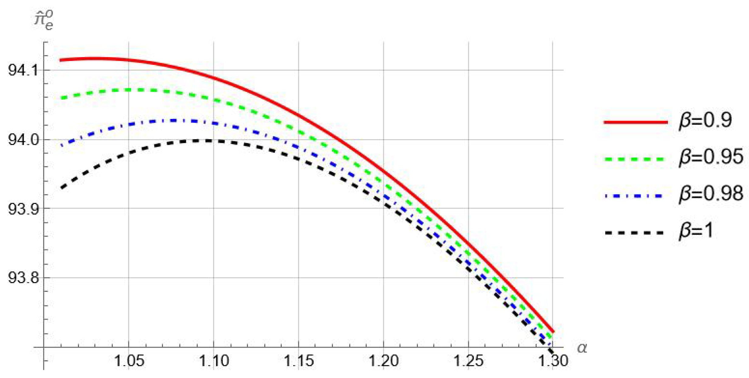
Proposition 5 examines whether overconfidence can benefit the supplier enough to positively impact the entire system, which includes both the supplier and the retailer. We calculate the system’s profit as ${\widehat{\pi }}_e^o:={\widehat{\pi }}_s^o+{\widehat{\pi }}_r^o$.

Proposition 5.

Suppose $v\left(\lambda \right)=\kappa ·\lambda$. Within a certain range of overconfidence levels, the system’s total profit ${\widehat{\pi }}_e^o$ increases as the overconfidence level rises.

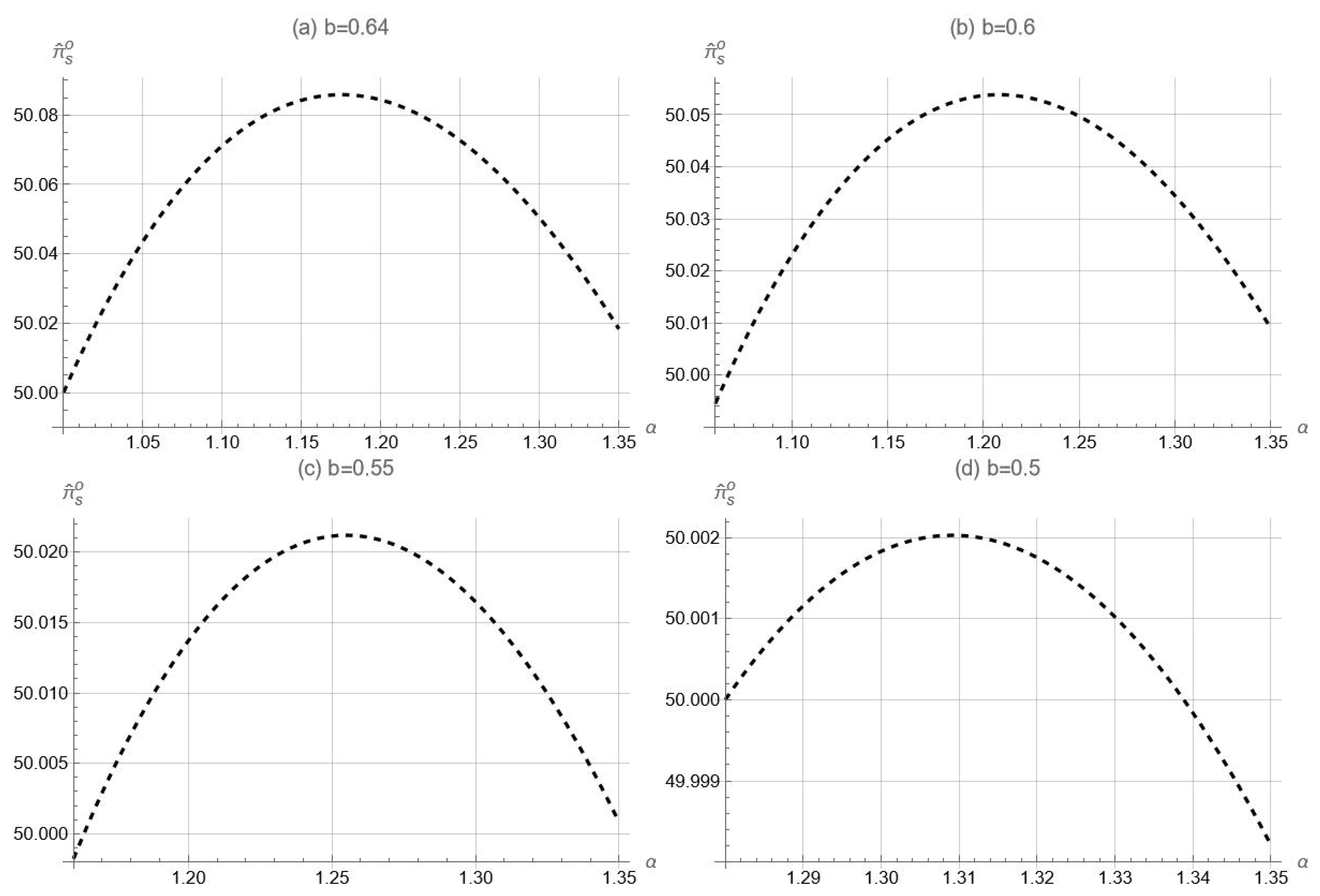
Proposition 5 indicates that, for the linear precision functions, retailer overconfidence can improve the system-wide performance within a certain range of overconfidence levels. Recall that overconfidence always hurts the retailer (Proposition 4a), while it can benefit the supplier (Proposition 4b). The enhanced system-wide performance demonstrated by Proposition 5 indicates that overconfidence can bring more benefits to the supplier than the harm it causes to the retailer. To check the robustness of this result, we plot how ${\widehat{\pi }}_e^o$ changes with respect to $\alpha$ in Figure 6 by assuming that $v\left(\lambda \right)=\kappa ·{\lambda }^{\beta }$. To ensure ${\widehat{\lambda }}^o>0$, we let ${\sigma }^2=42.5$ and $\kappa =0.4$. As per this figure, the system’s performance can improve as $\alpha$ increases for the non-linear accuracy functions, i.e., $\beta \ne 1$. Similar to Proposition 4b, the necessary condition for overconfidence to be beneficial, whether for the supplier or the system, is that the overconfidence level is relatively low. This low degree of overconfidence provides the retailer with a strong incentive to improve her forecast accuracy.

To understand and explore the intuition behind Proposition 5, we consider a centralized scenario where an overconfident central planner chooses an appropriate investment level to maximize the aggregate profit of both the supplier and the retailer. The forecast signal is transparent among the members of the supply chain. Given the signal s with subjective accuracy $\widehat{v}(\alpha ,\lambda )$, the total profit of the system is

$$p\left(a+{\displaystyle \frac{\widehat{v}(\alpha ,\lambda )s}{1+\widehat{v}(\alpha ,\lambda )}}-p\right)-\lambda .$$

It can be verified that the equilibrium price in this setting is $\widehat{p}(\lambda ,0)$, as shown in (5). Thus, the biased central planner behaves as if she sets the investment level to maximize

$$E\left[\widehat{p}(\lambda ,0)\left(a+{\displaystyle \frac{\widehat{v}(\alpha ,\lambda )s}{1+\widehat{v}(\alpha ,\lambda )}}-\widehat{p}(\lambda ,0)\right)-\lambda \right]={\displaystyle \frac{a^2}{4}}+{\displaystyle \frac{{\sigma }^2\widehat{v}(\alpha ,\lambda )}{4(1+\widehat{v}(\alpha ,\lambda ))}}-\lambda .$$

One can show that the equilibrium investment level for the biased central planner is $\widehat{\lambda }\left(\alpha \right)$, as defined in Proposition 1. Note that when $\alpha =1$, the centralized system can be viewed as a first-best benchmark. Accordingly, we call $\widehat{\lambda }(\alpha =1)$ the first-best investment level.

Proposition 6.

For a given α, $\widehat{\lambda }\left(\alpha \right)\ge {\widehat{\lambda }}^o\left(\alpha \right)$.

Proposition 6 shows that, for a given level of overconfidence, a biased centralized system invests more in forecasting than a decentralized system with information sharing. When $\alpha =1$, Proposition 6 further suggests that an unbiased decentralized system with information sharing underinvests in forecasting compared to the first-best level, $\widehat{\lambda }(\alpha =1)$. This underinvestment occurs because, in a decentralized system, the retailer only captures a fraction of the benefits from improved precision, reducing their incentive to invest. When the retailer is biased ($\alpha >1$), overconfidence can increase investment (Proposition 3b), moving it closer to the system-wide first-best level ($\widehat{\lambda }(\alpha =1)$). In this case, overconfidence helps mitigate the underinvestment caused by decentralization, thereby improving overall supply chain performance. As a result, the entire supply chain benefits from retailer overconfidence.

Overall, our findings offer a nuanced view of overconfidence in supply chains, showing that a certain level of retailer overconfidence can enhance system performance. Supply chain managers can foster positive overconfidence by providing resources that help retailers leverage their confidence constructively. The key challenge lies in identifying and maintaining an optimal level of overconfidence that maximizes system-wide benefits while avoiding negative effects.

6. Robustness Check

This section evaluates the robustness of our key insight—that is, retailer overconfidence can benefit the supplier and the entire supply chain. We first consider the scenario where the supplier can observe the retailer’s investment level (Section 6.1). Next, we explore the case where the supplier is fully aware of the retailer’s overconfidence (Section 6.2). In both extensions, the retailer’s investment policies remain consistent with Proposition 3. Given the complexity of deriving a closed-form solution for ${\widehat{\lambda }}^o$, we use numerical experiments to gain insights. Specifically, we specify the precision function as (6) with ${\sigma }^2=42.5$ and $\kappa =0.4$, which ensures positive ${\widehat{\lambda }}^o$ for any $\alpha >1$.

6.1. Observable Investment

With information sharing, the retailer discloses the signal s to the supplier, claiming its accuracy as $\widehat{v}(\alpha ,{\widehat{\lambda }}^o)$. However, the supplier observes the actual investment level ${\widehat{\lambda }}^o$ and, knowing the true precision function $v\left(\lambda \right)$, correctly anticipates the forecast’s accuracy as $v\left({\widehat{\lambda }}^o\right)$ rather than the claimed $\widehat{v}(\alpha ,{\widehat{\lambda }}^o)$. Given the investment level ${\widehat{\lambda }}^o$, the supplier sets the wholesale price $w^o\left({\widehat{\lambda }}^o\right)$ as defined in (7) and the equilibrium retail price $\widehat{p}({\widehat{\lambda }}^o,w^o)$ as defined in (5). Based on these results, the retailer’s expected profit is ${\widehat{\pi }}_r^b:=E\left[{\pi }_r(\widehat{p},w^o,{\widehat{\lambda }}^o)\right]$, the supplier’s expected profit is ${\widehat{\pi }}_s^b:=E\left[{\pi }_s(\widehat{p},w^o,{\widehat{\lambda }}^o)\right]$, and the total supply chain profit is ${\widehat{\pi }}_e^b:={\widehat{\pi }}_r^b+{\widehat{\pi }}_s^b$.

We plot the performance of the retailer, supplier, and system in Figure 7 for varying $\beta$. Figure 7a,b show that both the supplier and the system benefit from overconfidence, confirming that our key insights hold even when the supplier observes the investment level. However, as shown in Figure 7c, the retailer continues to suffer from overconfidence, consistent with the case of non-observable investments, where overconfidence invariably leads to self-harm.

6.2. Sophisticated Supplier

In practice, a monopoly supplier often possesses expertise in understanding the retailer’s identity. This means the supplier is sophisticated—unbiased and fully aware of the retailer’s overconfidence. Anticipating the biased investment level ${\widehat{\lambda }}^o$ and the equilibrium retail price $\widehat{p}({\widehat{\lambda }}^o,w)$, the sophisticated supplier’s problem becomes

$$\underset{w}{max}\left\{w\left[a+{\displaystyle \frac{v\left({\widehat{\lambda }}^o\right)·s}{1+v\left({\widehat{\lambda }}^o\right)}}-\widehat{p}({\widehat{\lambda }}^o,w)\right]\right\}.$$

By solving this, we obtain the equilibrium wholesale price as

$$w^f\left({\widehat{\lambda }}^o\right):={\displaystyle \frac{a}{2}}+{\displaystyle \frac{v\left({\widehat{\lambda }}^o\right)s}{1+v\left({\widehat{\lambda }}^o\right)}}-{\displaystyle \frac{\alpha v\left({\widehat{\lambda }}^o\right)s}{2\left(1+\alpha v({\widehat{\lambda }}_o\right))}}.$$

Here, we assume the value of signal s is sufficiently small relative to market potential a to ensure the regularity of $w^f\left({\widehat{\lambda }}^o\right)$. Let the retailer’s profit be ${\widehat{\pi }}_r^f:=E\left[{\pi }_r(\widehat{p},w^f,{\widehat{\lambda }}^o)\right]$ and the supplier’s profit be ${\widehat{\pi }}_s^f:=E\left[{\pi }_s(\widehat{p},w^f,{\widehat{\lambda }}^o)\right]$. Thus, the total system profit is ${\widehat{\pi }}_e^f:={\widehat{\pi }}_r^f+{\widehat{\pi }}_s^f$.

Although analytically assessing the impact of overconfidence on supplier and system performance is challenging, our numerical analysis confirms the main findings—that is, overconfidence can benefit both the supplier and the entire supply chain. Specifically, within a certain range of overconfidence levels, increasing retailer overconfidence enhances the profits of both the supplier and the system, as shown in Figure 8a,b.

Proposition 7.

When the retailer shares the forecast with a sophisticated supplier, the retailer’s performance can improve with increasing overconfidence.

In contrast to Proposition 2, Proposition 7 suggests that overconfidence does not always result in self-harm. To illustrate this, we plot the retailer’s profit in Figure 9. As per this figure, the retailer’s profit increases with overconfidence, particularly at lower levels of bias. Additionally, the range of overconfidence levels where the retailer benefits expands as $\beta$ increases. This challenges the conventional view of overconfidence as inherently detrimental, highlighting that in contexts like information sharing with a sophisticated supplier, overconfidence can enhance retailer performance.

For insight, overconfidence has two opposing effects on the retailer. The first (direct) effect is negative, as greater overconfidence exacerbates distortions in forecasting investments and retail pricing decisions (Proposition 2). Conversely, overconfidence can increase investment level when subjective forecast accuracy is low (Proposition 3b), enabling the sophisticated supplier to mitigate pricing distortions by setting a more accurate wholesale price. Thus, the second (indirect) effect is positive. When overconfidence is relatively low, the positive indirect effect outweighs the weaker direct negative effect, allowing the retailer to benefit from her overconfidence.

7. Conclusions, Discussion, and Managerial Insights

This study investigates the direct effects of retailer overconfidence on supply chain efficiency and explores how structural factors—such as investment transparency and supplier sophistication—shape outcomes. Overconfidence manifests when the retailer overestimates her ability to generate precise demand forecasts through investments. Our analysis reveals three key insights:

• Investment incentives: overconfidence amplifies the retailer’s motivation to invest in forecasting, particularly when forecasts are subjectively perceived as imprecise.
• Information sharing dynamics: Without Information Sharing: Overconfidence harms both the retailer and the supply chain, as distorted investment decisions reduce profitability. With information sharing, overconfidence counterintuitively enhances supply chain performance by mitigating underinvestment caused by decentralized decision-making.
• Sophisticated suppliers: When suppliers account for the retailer’s cognitive bias (sophistication), a win–win outcome emerges. The supplier adjusts pricing strategies to counteract the retailer’s overinvestment, benefiting both parties. Supplier sophistication thus acts as a moderating force, neutralizing the retailer’s self-harming behavior.

In sum, overconfidence’s impact is context-dependent, shifting from detrimental to beneficial based on supply chain coordination mechanisms. Further, strategic information sharing and supplier adaptability are critical to harnessing overconfidence’s paradoxical advantages.

7.1. Discussion

Our findings contribute to the growing literature on behavioral operations and forecast investment by explicitly modeling the impact of overconfidence on information acquisition decisions. In contrast to classical models of forecast investment, which typically assume fully rational agents optimizing under known distributions, our model introduces biased belief formation as a key determinant of investment behavior. This departure reveals that overconfident retailers may either over- or under-invest in forecast precision, depending on their perceived signal quality, leading to systematically different investment levels and supply chain outcomes than those predicted by rational benchmark models.

Furthermore, our work is closely related to the behavioral operations literature that examines cognitive biases in supply chain contexts, such as anchoring [54] and Dunning–Kruger Effect [55]. These studies demonstrate that biased beliefs often result in persistent inefficiencies in ordering or contracting decisions. Our model complements this stream by focusing specifically on forecast investment—a domain where belief distortions about signal precision play a pivotal role—and by analytically characterizing how overconfidence alters the value and timing of information acquisition.

Finally, our theoretical predictions are consistent with empirical and experimental findings in behavioral decision-making. For instance, the non-monotonic relationship we identify between overconfidence and supply chain performance aligns with experimental results showing that moderate overconfidence can lead to motivated effort and beneficial risk-taking, while excessive bias reduces judgment accuracy and impairs coordination (e.g., [31]). This reinforces the practical insight that the effects of overconfidence are context-dependent, and interventions must be carefully calibrated to avoid both under- and over-reaction to perceived forecast value.

By situating our findings within these three complementary streams—rational investment models, cognitive bias research, and empirical observations—we provide a more nuanced understanding of how behavioral distortions interact with information structures in operational settings.

7.2. Managerial Insights

The findings of this study offer several actionable insights for supply chain managers.

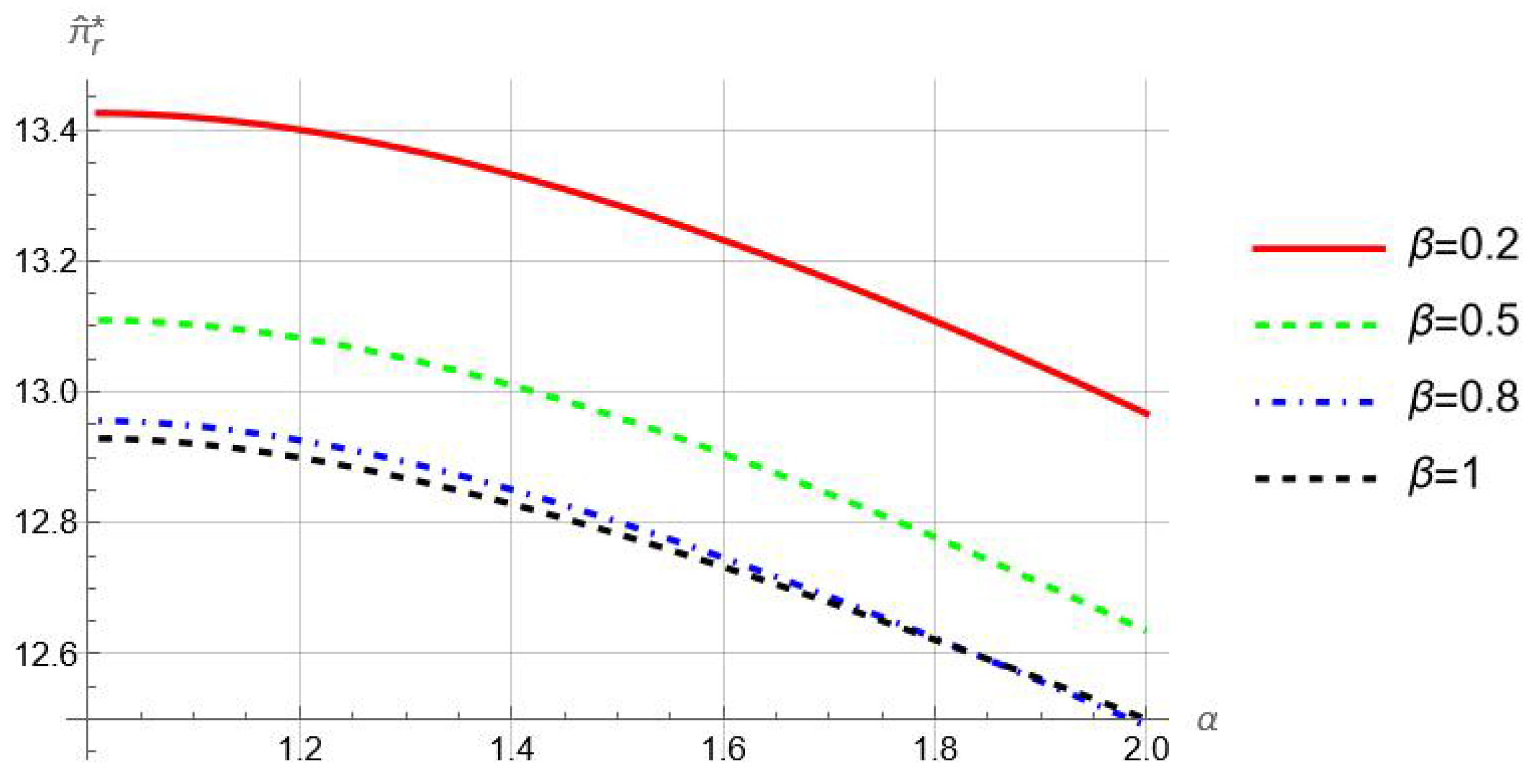
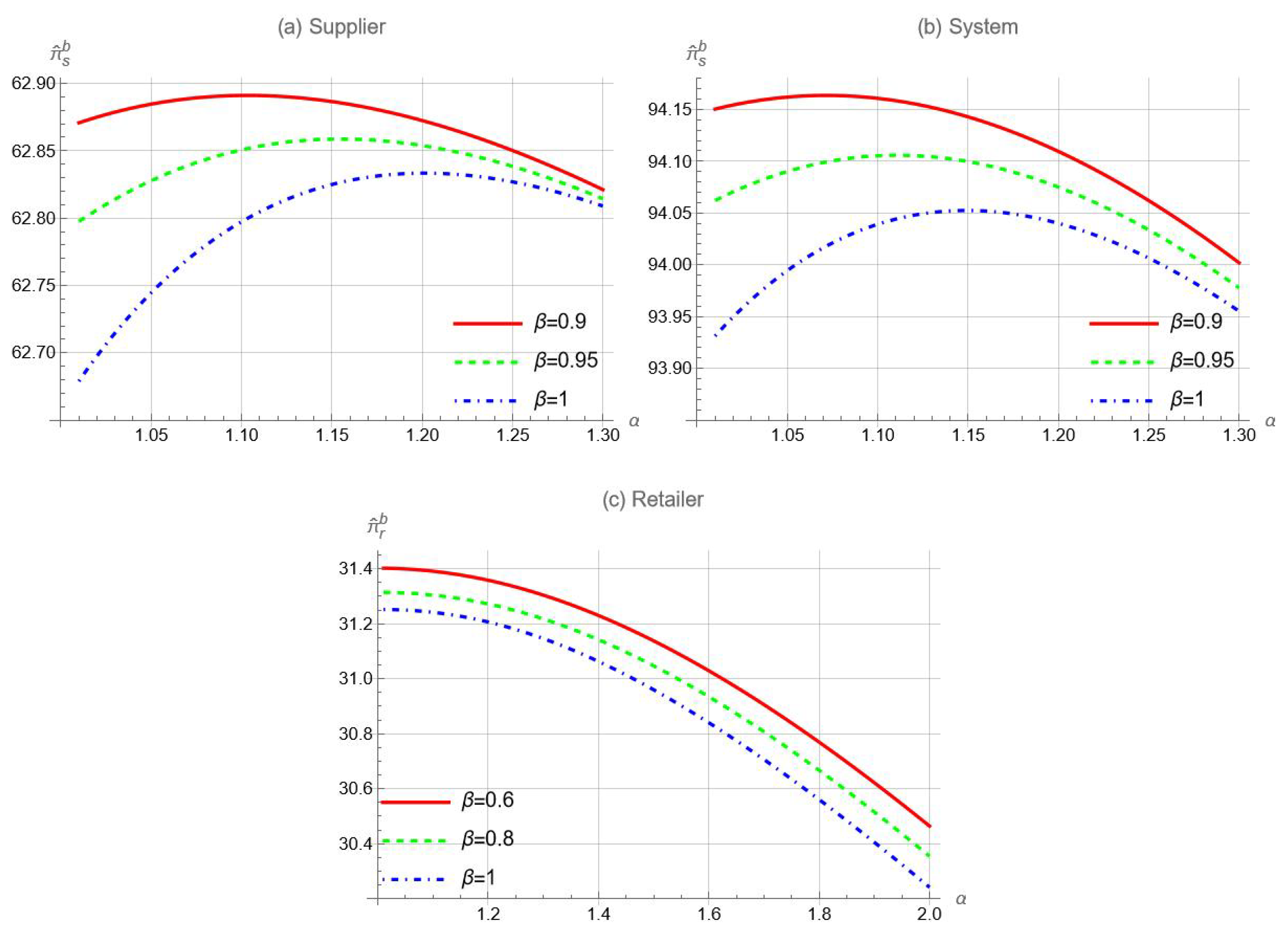
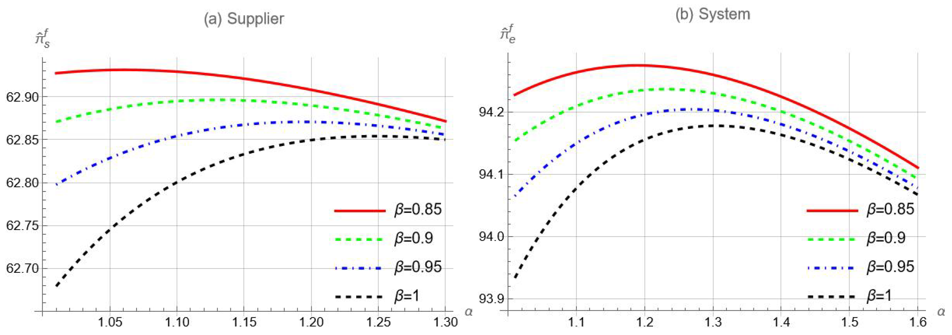
First, retailers must carefully evaluate whether and when to mitigate overconfidence. As overconfidence can either help or hinder forecast investment, depending on the decision environment, mitigation strategies should also be context-dependent. Our findings suggest corrective mechanisms (e.g., calibration training or incentive design) might be necessary to mitigate excessive overconfidence in scenarios without information sharing (Proposition 2). However, in supply chains with information sharing, reducing overconfidence may harm the retailer’s performance, especially with a sophisticated supplier (Proposition 7). Instead of fully eliminating overconfidence, reducing it to a manageable level emerges as a more effective strategy when supplier sophistication is present.

Second, suppliers and upstream partners can benefit from anticipating behavioral tendencies among their downstream counterparts. Our analysis shows that moderate overconfidence can benefit both the supplier and the entire supply chain under information sharing (Propositions 4b and 5). These findings highlight the importance of effective information sharing in enhancing supply chain performance and leveraging the potential positive effects of overconfidence. Understanding that some retailers may consistently over- or under-invest due to biased beliefs allows supply chain partners to proactively adjust their collaboration strategies, such as by sharing forecasts, offering data-driven insights, or structuring contracts that account for informational asymmetries.

The effective application of our managerial insights hinges on accurately assessing the degree of overconfidence. Retailers with high overconfidence should prioritize implementing mitigation programs. Similarly, if suppliers can precisely measure the retailer’s overconfidence, this bias can benefit individual supply chain members and the entire supply chain under an information-sharing strategy. Thus, accurately quantifying overconfidence is critical for leveraging our findings effectively.

The literature offers various methods to measure overconfidence. These include the following:

• Survey-based self-assessment tools, where individuals are asked to estimate their own forecasting accuracy or rank their ability relative to others, e.g., [31]. These are widely used in behavioral research to capture overplacement and overprecision.
• Calibration tests from experimental economics and psychology, which compare subjective confidence intervals with actual outcomes to assess the degree of miscalibration, e.g., [56].
• Prediction tasks: predict subjective performance across ability distributions and compare with objective (actual) results, as proposed by [55], which can reveal systematic overestimation of one’s own competence.

Recognizing overconfidence as a stable cognitive bias, managers can use these established measures to evaluate its degree. Understanding overconfidence levels enables informed decision-making, optimizing performance in response to this bias.

7.3. Future Research

This study opens several promising avenues for future research in the domain of behavioral supply chain management. While our theoretical model provides foundational insights into how overconfidence affects forecast investment decisions and supply chain outcomes, further work is needed to validate and extend these findings in more applied settings.

First, the empirical relevance of the model can be explored through experimental and field-based validation. For example, controlled laboratory experiments could be designed to simulate forecast investment environments where participants make decisions under varying degrees of confidence and information availability. Such experiments would allow for the systematic observation of behavioral deviations from rational benchmarks and help test the model’s predictions, such as the non-monotonic relationship between overconfidence and system performance.

Second, while we focus on overconfidence as the primary cognitive bias, other behavioral factors may also play important roles in shaping forecast investment decisions. For instance, loss aversion may cause managers to under-invest in information to avoid the perceived risk of wasted effort, while confirmation bias could lead decision-makers to selectively attend to signals that reinforce their prior beliefs. Similarly, ambiguity aversion may reduce willingness to invest in forecasts when signal reliability is uncertain. These biases can interact with overconfidence in complex ways, potentially amplifying or mitigating its effects. Future research could explore multi-bias behavioral models to capture these interactions and offer a more holistic view of bounded rationality in operational decision-making.