Integrating Uncertainties in a Multi-Criteria Decision Analysis with the Entscheidungsnavi

Abstract

The Entscheidungsnavi is an open-source decision support system based on multi-attribute utility theory, that offers various methods for dealing with uncertainties. To model decisions with uncertainties, decision-makers can use two categories: Forecast and Parameter Uncertainties. Forecast Uncertainty is modeled with (combined) influence factors using discrete, user-defined probability distributions or predefined ‘worst-median-best’ distributions. Parameter Uncertainty allows imprecision for utilities, objective weights, and probability distributions. To analyze these uncertainties, the Entscheidungsnavi offers several methods and tools, like a robustness check, based on (Monte Carlo) simulations and a sensitivity analysis. The objective weight analysis provides insights into the effects of different objective weight combinations. Indicator impacts, tornado diagrams, and risk profiles visualize the impact of uncertainties in a decision under risk. Risk profiles also enable a check for stochastic and simulation dominance. This article presents the complete range of methods for dealing with uncertainties in the Entscheidungsnavi using a hypothetical case study.

1. Introduction

Extensive research over the years has led to a plethora of different Multi-Criteria Decision-Making (MCDM) methods, whose strengths and limitations have been analyzed in numerous studies (e.g., [1,2]) and meta-studies [3]. In practice, software tools regularly accompany the application of these methods. The overview of the International Society on MCDM (https://www.mcdmsociety.org/content/software-related-mcdm-0, accessed on 30 March 2024) currently lists 28 tools, the majority of which are freely available. Most tools are based on a particular methodology, but a few offer a choice of methods (e.g., DEFINITE (https://spinlab.vu.nl/support/tools/definite-bosda/, accessed on 30 March 2024)).

Only a small number of MCDM tools focus on multi-attributive value or utility theory (MAVT/MAUT). MACBETH (https://m-macbeth.com, accessed on 30 March 2024) [4,5,6], for example, is a commercial decision support system (DSS) that has already been used in many different application contexts (e.g., [7,8,9]). FITradeoff (https://fitradeoff.org/, accessed on 30 March 2024) [10,11] and the Entscheidungsnavi (https://enavi.app/, accessed on 30 March 2024) [12] are available at no cost.

Decision-makers (DMs) seeking a method and software for their MCDM problems face a dilemma between ease of use and the quality of the decision recommendation. In general, the MAUT methodology [13] is considered demanding and difficult due to the trade-offs between objectives that need to be assessed. To reduce the application hurdles and avoid overwhelming the DM, certain methodologies, such as AHP [14] and outranking methods [15], are based on clear and simple queries. This also includes fuzzy methods [16,17], which deliberately anticipate a certain degree of fuzziness in the model. DMs can use these methods without having knowledge of the underlying algorithms. Although these lower demands on the DM reduce application hurdles and are often methodologically elegant, this can be at the expense of quality.

To achieve high decision quality, the DM needs to reflect on the decision problem. First of all, it is important to structure the decision situation, i.e., to clearly formulate the decision statement, analyze the fundamental objectives, and creatively develop alternatives [18,19]. Back in the 1990s, Keeney introduced the concept of Value-Focused Thinking (VFT), which has proven itself in many practical applications (e.g., [20,21,22]. If DMs are not supported during this phase of structuring, there is a risk that the problem will not be properly defined [23], the objectives will be incomplete or not fundamental [24], and potentially attractive alternatives will be overlooked [25].

Secondly, DMs must research and use relevant and reliable information. Furthermore, an evaluation or decision should be based on comprehensible logic and the DM’s identified preferences [19]. A transparent and comprehensible process prevents a black-box character, enabling the reflection of the DM’s preferences. MAUT has clear advantages over most other methods in this respect. The reason for this can be explained by the comparatively simple and strictly decomposition mathematics combined with a theoretically clean foundation [13]. Although the trade-offs between objectives required by MAUT are—as mentioned above—difficult to determine, they can be clearly interpreted in terms of content without further fuzziness. In addition, possible effects on the result are generally easy to understand. In terms of clarity and comprehension, MAUT is an evaluation logic that is highly reflective and transparent.

MAUT enables the consideration of uncertainties in various ways. This concerns not only the integration of risk preferences in utility functions based on axioms [26] but also the possibility of easily integrating various standard methods for dealing with uncertainties into the model. Which methods are suitable here and what an extension of these methods should look like should be based on how beneficial this integration is for the desired reflection of the DM. When faced with uncertainty, DMs can ask themselves, for example, the following questions to reflect on the decision situation: Are the parameters I have entered aggregated in a comprehensible and plausible way to produce a valid result? Are the uncertainties considered in the model exactly the uncertainties that may have a decisive influence on the result? To what extent can the respective uncertainties have a positive or negative impact on the result? Which uncertainties have the greatest influence on the result?

The Entscheidungsnavi is, as far as we know, the only DSS that comprehensively supports the DM in structuring decision-making situations, applying a transparent mathematical method for calculating the best alternative, and addressing these questions with regard to uncertainties. In the decision front-end, VFT [18] is used to structure the decision situation and identify the first pieces of relevant information (objectives and alternatives). In his recent book, Keeney [27] also refers to the Entscheidungsnavi as the only tool comprehensively supporting VFT. In the decision back-end, the concept of MAUT [13] is used to find the best alternative under uncertainty. In addition, the Entscheidungsnavi offers many different evaluation methods that allow the DM to reflect on and analyze their results.

In this paper, we present how to deal with uncertainties and how to analyze the questions mentioned above in the Entscheidungsnavi using a simple hypothetical case study. Therefore, we briefly introduce the Entscheidungsnavi (Section 2) and a case study (Section 3) that is constructed to show all available analysis tools and options for facing uncertainties in the following sections. In Section 4, we explain the implementation of MAUT in the Entscheidungsnavi, and in Section 5, we show how uncertainties can be modeled in the DSS. In Section 6, Section 7, Section 8 and Section 9, we present the following various analysis tools with which uncertainties can be examined more closely by the DM: methods for checking the robustness of the result (Section 6), objective weight analysis (Section 7), sensitivity analysis (Section 8), and indicator impacts, tornado diagrams, and risk profiles (Section 9). In Section 10, we conclude the paper and point out limitations in dealing with uncertainties in the Entscheidungsnavi.

2. The Entscheidungsnavi—A Decision Skill Trainer

The Entscheidungsnavi [12] is an open-source web tool that helps DMs make well-thought-out decisions and improve their decision-making competence. The first version of the tool was developed in 2017 for teaching purposes as part of the ‘Decision Theory’ course at RWTH Aachen University. In the following years, a group of computer science students worked continuously on implementing functionalities, improving usability, and incorporating extensive user feedback. The Entscheidungsnavi is now used by other universities and institutions for teaching and advisory purposes due to its high level of professionalization. As a non-profit project, this DSS is available at no cost to all users. To make this possible, the Entscheidungsnavi is supported by a non-profit organization (Reflektiert Entscheiden e.V. (https://reflektiert-entscheiden.de, accessed on 30 March 2024)) with users from various universities in Germany and Austria and a strategic management consultancy firm that uses the tool for consulting projects. Feedback from practical applications in the form of functionality requests flows directly into further development of the tool. This paper refers to the current version, 8.2.2; further versions with extended functions are already in development.

The Entscheidungsnavi is based on the approach of reflective decision-making [28] and consists of five successive steps: the formulation of the decision statement (1), the development of the fundamental objectives (2), the identification of alternatives (3), the establishment of a consequences table (4), and evaluation on the basis of preferences (5). The first three steps support the user in structuring the decision-making situation using the concept of VFT by Ralph Keeney [18]. VFT follows the idea that decisions should be approached proactively: i.e., decision situations should be seen as opportunities to shape something with foresight. Therefore, the first step promotes a broad and open formulation of the decision statement, which paves the way for a correspondingly large scope for action. The Entscheidungsnavi supports DMs in formulating a proactive decision statement by helping them reflect on their own values and asking several probing questions. In the second step, DMs should develop their fundamental objectives. Therefore, the second step requires DMs to brainstorm important aspects and intensively scrutinize all collected aspects in order to precisely define them. The Entscheidungsnavi supports DMs in developing the fundamental objectives by providing context-related master lists of objectives and an option to create an objective hierarchy. When identifying possible alternatives in the third step, VFT calls for a high degree of creativity in order to find or design new attractive alternatives. The fundamental objectives that have already been formulated should always be kept in mind so that a high level of attractiveness is achieved when designing new alternatives. The Entscheidungsnavi supports DMs with the following creativity techniques: finding weaknesses of known alternatives, performing an objective-focused search, and developing a strategy table. In the fourth step, DMs should establish the consequences table, in which biases [29] should be avoided. The Entscheidungsnavi informs DMs about these biases and thus sensitizes them when evaluating the consequences and possible uncertainties. In the final step, the DMs’ preferences are included in the model on the basis of MAUT. This is implemented by using utility functions and trade-offs to determine the objective weights. The tool supports DMs with the help of graphic illustrations and explanations of the functions. Finally, the Entscheidungsnavi offers a wide range of evaluation options to analyze and reflect on the final ranking of the alternatives in more detail. In this paper, we focus on the fourth and fifth steps, as the structuring phase of a decision situation does not affect uncertainties with regard to MAUT.

The Entscheidungsnavi places great emphasis on user-friendliness and an intuitive interface so that everyone can use the web tool. As not all DMs are familiar with the use of MCDM and MAUT, the Entscheidungsnavi is available in three variants: Starter, Educational, and Professional. The Starter variant is deliberately kept simple and, therefore, has a greatly reduced range of methods and functionalities. It is ideal for DMs who have no prior experience in MCDM and want to quickly obtain a first impression of the process. The focus in this version is on structuring the decision situation. The Educational variant guides DMs through the reflective decision-making process in small steps, supported by extensive explanations and background information. These cover the basics of decision theory, operating instructions, and tips and tricks for the respective step. This version is particularly suitable for DMs who want to deal intensively with all aspects of a reflective decision and improve their decision-making skills. Previous knowledge about MCDM is not necessary in this version either. The Professional variant provides a similar feature set to the Educational variant but does so without guiding DMs and with fewer explanations. This variant is, therefore, suitable for those who are familiar with the implemented tools and methods and simply want to solve a decision problem efficiently. All variants are based on requests and suggestions from DMs in the field.

3. Case Study

To subsequently explain the mathematical models and functionalities of the Entscheidungsnavi regarding the handling of uncertainties, we would first like to briefly introduce a case study in this section. It is important to note that this case study is a highly simplified model of a logistics decision and was solely created to explain how DMs can deal with and analyze uncertainties using the Entscheidungsnavi.

258 GmbH, a company that sells on-site-stored wood, would like to expand as part of its growth strategy. For this purpose, it is looking for a new location in North Rhine-Westphalia (NRW), Germany. The company’s decision statement is as follows: ‘Which location best suits the new wood warehouse with adjoining wood sales for 258 GmbH?’

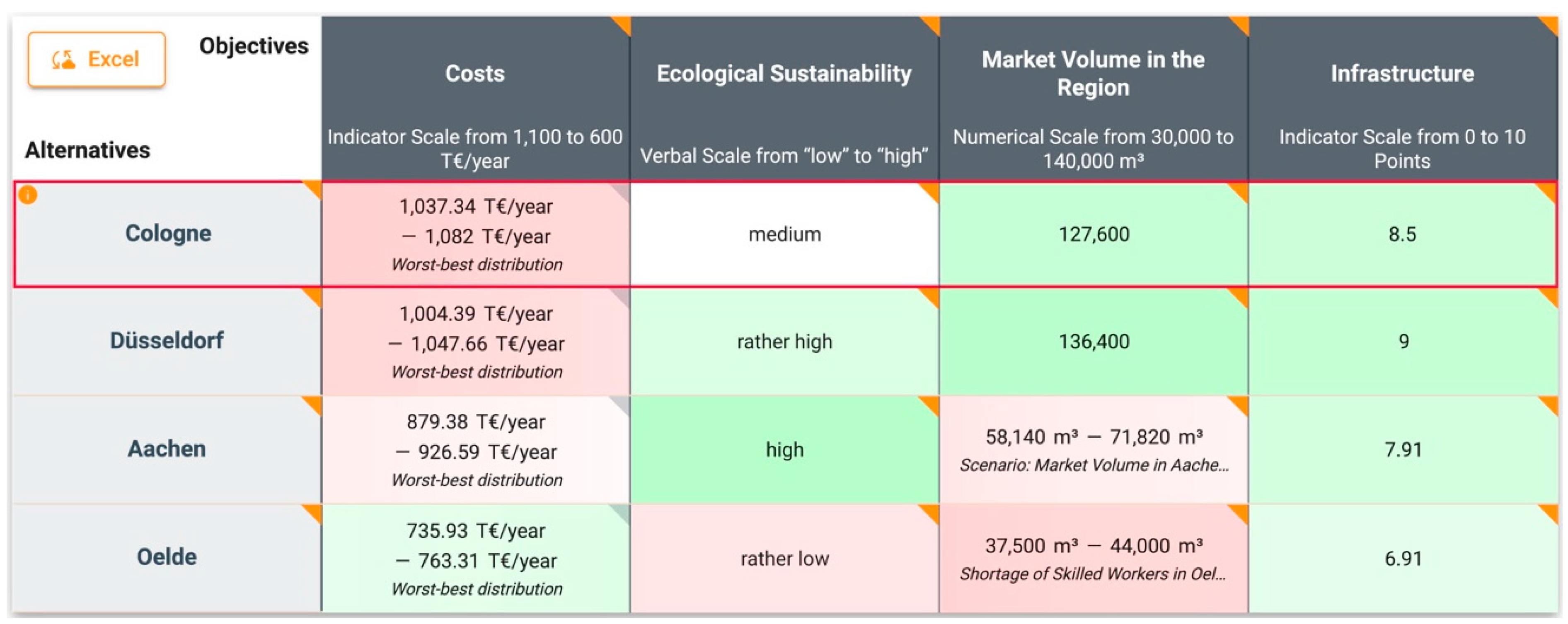
The company has already defined the objectives and alternatives of the decision statement and determined how well the alternatives fulfill the objectives in a consequences table (see Figure 1).

Figure 1. Consequences table for the decision statement ‘Which location best suits the new wood warehouse with adjoining wood sales for 258 GmbH?’. Good consequences are displayed in green, while average ones are displayed in white and bad ones are displayed in red.

258 GmbH defines four fundamental objectives: Costs, Ecological Sustainability, Market Volume in the Region, and Infrastructure.

The objective Costs deals with the expected annual costs for the operation of their wood sales business, including the wood warehouse, which, among other expenses, are costs for rent, the property lease, interest costs and loan repayment costs for the property, personnel costs, taxes and duties, and maintenance and operating costs. The model does not consider transport costs and sales tax, as they will be passed on to the customer through an increased retail price based on the location of the warehouse. The objective is measured using an indicator scale from 1100 T€/year (worst value) to 600 T€/year (best value), which is made up of five indicators: Personnel costs (€/month), Rent/Loan payment (€/month), Property tax (€/quarter), Electricity costs (€/year), and Other operating & maintenance costs (€/month).

The objective Ecological Sustainability evaluates properties at different locations based on their ecological sustainability. It is measured using a verbal scale from low (worst value) to high (best value), with five verbal levels.

The objective Market Volume in the Region is measured in terms of the expected volume of construction wood sold in m³. This takes two factors into account: geographical reach and competition. In large cities, we assume that residents travel a maximum distance of 50 km to buy wood. In more rural areas, we assume that residents travel up to 100 km to buy wood, as residents there are used to traveling longer distances to make purchases. To assess competition, we consider the extent of potential competition at the locations. We assume that there is already an abundance of wood merchants, particularly in urban centers. The objective is measured on a numerical scale from 30,000 m³ (worst value) to 140,000 m³ (best value).

The last objective, Infrastructure, is made up of two indicators: Current state of infrastructure and Expected future state of infrastructure. These indicators are used to assess the infrastructure at each location in terms of its quality and possible restrictions (e.g., due to extensive construction sites) now and in the future. Aspects such as highway connections, railways, shipping routes, and the general volume of traffic in the region are evaluated holistically. Airports are not considered in this model, as airplanes are not suitable for transporting the goods offered. The objective is measured using an indicator scale that ranges from 0 (worst value) to 10 points (best value).

Furthermore, 258 GmbH has already limited its choice of alternatives to four locations: Cologne, Düsseldorf, Aachen, and Oelde. Each alternative represents a specific property in the city. As the largest city in the Rhineland, Cologne offers excellent infrastructure with major highways, the Rhine port for transporting goods, and a lot of craftsmen and construction companies nearby. Düsseldorf, the state capital of NRW, has a strong economy, a well-developed road network, and a high density of construction sites. Aachen is located in the west of NRW, bordering Belgium and the Netherlands, which offers the strategic advantage of being able to sell to people from three countries. The region is also characterized by a decent amount of construction activity. Oelde is a small town in the east of NRW. The town is characterized by its excellent connection to the highway and offers the opportunity to set up a medium-sized wood warehouse.

The performance of the alternatives is assessed with regard to all objectives on the respective objective’s scale in the consequences table (see Figure 1). As some consequences are uncertain and depend on external factors, several influence factors are used. Examples of influence factors are the worst–best distribution, which is used to model a kind of general uncertainty regarding consequences, or the ‘Shortage of Skilled Workers’ in Oelde. In the following sections, we will discuss these uncertainties and the different methods with which to analyze them in the Entscheidungsnavi in more detail.

4. The Implementation of MAUT in the Entscheidungsnavi

The mathematical model of the Entscheidungsnavi is based on the additive utility function of MAUT, which is used to determine the best alternative in multi-criteria decisions under uncertainty [13,30,31]. In this model, alternatives are compared and ranked according to their utility. The alternative with the highest utility is regarded as the best and should be chosen by the DM. To use the additive model, DMs must first define a set of objectives $\mathbb{O}=\left\{O_1,\dots ,O_I\right\}$ and a set of alternatives $\mathbb{A}=\left\{A_1,\dots ,A_J\right\}$ for some natural numbers $I,J$ for the decision situation. Subsequently, they have to evaluate the consequences $x_{ij}$ of all $J$ alternatives in the respective $I$ objectives with $1\le i\le I$ and $1\le j\le J$ in a consequences table. The utility of each alternative $A_j$ is calculated using Formula (1) for the additive expected utility [26,32].

$$EU\left(A_j\right)={\sum }_{i=1}^I{w}_i\left[{\sum }_{k=1}^{K_{ij}}P\left(s_{ij}^k\right)U_i\left(x_{ij}^k\right)\right]$$

(1)

$${\sum }_{i=1}^I{w}_i=1$$

(1a)

$${\sum }_{\mathrm{k}=1}^{{\mathrm{K}}_{\mathrm{i}\mathrm{j}}}\mathrm{P}\left({\mathrm{s}}_{\mathrm{i}\mathrm{j}}^{\mathrm{k}}\right)=1$$

(1b)

Here, $w_i$ represents the weight of objective $O_i$. The sum of all objective weights must equal one (1a). Objective weights are determined using the trade-off method [13] in the Entscheidungsnavi. To model decisions under uncertainty, we have different states $s_{ij}^k$ that occur with corresponding probabilities $P\left(s_{ij}^k\right)$ and result in some consequences $x_{ij}^k$, with $1\le k\le K_{ij}$. So, if $K_{ij}=1$, the state $s_{ij}^1$ occurs with a probability of 100 percent, and therefore, $x_{ij}^1$ is a certain consequence. If $K_{ij}\ge 2$, the consequence $x_{ij}$ is uncertain. This is the case when influence factors are included in the model (see Section 5.1). The probabilities of all states for every $ij$ add up to one (1b). Finally, $U_i$ represents the utility of objective $O_i$. Utilities are used to map the DM’s preferences.

In the Entscheidungsnavi, the utilities of the consequences are determined differently for objectives with a verbal scale than for objectives with a numerical scale. The utilities for objectives with verbal scales are determined using discrete utilities, as shown in Formula (2a), while for objectives with numerical scales, the utilities are determined using the exponential utility function, as shown in Formula (2b). For a more thorough explanation of how the utilities in the Entscheidungsnavi are determined, see von Nitzsch et al. [12].

Discrete utilities for objectives with a verbal scale:

$$U_i\left(x_{ij}^k\right)=\left\{\begin{array}{cccc}0& & & if\hspace{0.17em}{x}_{ij}^k=x_i^{-}\hfill \\ DR\left(x_{ij}^k\right)& & & if\hspace{0.17em}{x}_{ij}^k\in (x_i^{-},x_i^{+})\hfill \\ 1& & & if\hspace{0.17em}{x}_{ij}^k=x_i^{+}\hfill \end{array}\right.$$

(2a)

Exponential utility function for objectives with a numerical scale:

$$U_i\left(x_{ij}^k\right)=\left\{\begin{array}{lllll}\frac{1-e^{-c_i\frac{x_{ij}^k-x_i^{-}}{x_i^{+}-x_i^{-}}}}{1-e^{-c_i}}& & & if& c_i\ne 0\\ \frac{x_{ij}^k-x_i^{-}}{x_i^{+}-x_i^{-}}& & & if& c_i=0\end{array}\right.$$

(2b)

All consequences $x_{ij}^k$ for objective $O_i$ must lie within the interval $\left[x_i^{-},x_i^{+}\right]$, which is defined by the DM and represents the measurement scale for the objective. While $x_i^{-}$ represents the consequence with the lowest utility (zero), and $x_i^{+}$ is the consequence with the greatest utility (one), the utility $U_i\left(x_{ij}^k\right)$ increases as the consequences $x_{ij}^k$ improve. The exact utility of the consequence levels is determined by the DM via direct rating; therefore, the utility for the consequence $x_{ij}^k$ is represented by the direct rating function $DR\left(x_{ij}^k\right)$. $c_i$ represents the risk aversion parameter for objective $i$. In some instances, the numerical value of $x_i^{+}$ can be smaller than that of $x_i^{-}$. This happens when inverted scales are used, which is, e.g., the case for cost objectives, where lower costs yield a higher utility.

It is also possible to measure the consequences of every objective using several numerical indicators $1\le q\le Q$ (indicator scale). In this case, the consequences $x_{ij}^k$ are not assessed directly but rather through the consequences for the respective indicators $x_{ijq}^k$ for all $Q$ indicators. Indicator consequences can be aggregated using either an additive-weighted composition or a user-defined formula. Formula (3) shows the calculation of consequences using an additive-weighted composition:

$$x_{ij}^k={\sum }_{q=1}^Q\left[x_i^{-}+\frac{x_{ijq}^k-x_{iq}^{-}}{x_{iq}^{+}-x_{iq}^{-}}(x_i^{+}-x_i^{-})\right]\frac{g_q}{{\sum }_{v=1}^Q{g}_v}$$

(3)

The interval $\left[x_{iq}^{-},x_{iq}^{+}\right]$ represents the indicator’s measurement scale and defines the possible range of consequences for the $q$-th indicator of objective $O_i$. Furthermore, $g_q$ represents the weight of the $q$-th indicator and can be any positive number. Similarly to the range of the consequence’s scale, $x_{iq}^{-}$ describes the consequence with the lowest utility of the $q$-th indicator, and $x_{iq}^{+}$ describes the consequences with the highest utility. Therefore, $x_{iq}^{+}$ can have a lower numerical value than $x_{iq}^{-}$ for inverted indicator scales. If a user-defined formula is chosen, the DM can decide whether the range of the aggregated scale should be automatically calculated or defined by the DM. The utilities for objectives that are measured using an indicator scale are determined using the exponential utility function in Formula (2b).

In the case study, the objectives Costs and Infrastructure are measured using an indicator scale. For the latter, the individual indicator consequences are aggregated additively according to their weights, as shown in Formula (3). In the objective Costs, the indicator consequences are aggregated according to a user-defined formula to determine the total costs per year. Therefore, five indicators are used: Personnel costs (€/month), Rent/Loan payment (€/month), Property tax (€/quarter), Electricity costs (€/year), and Other operating & maintenance costs (€/month). 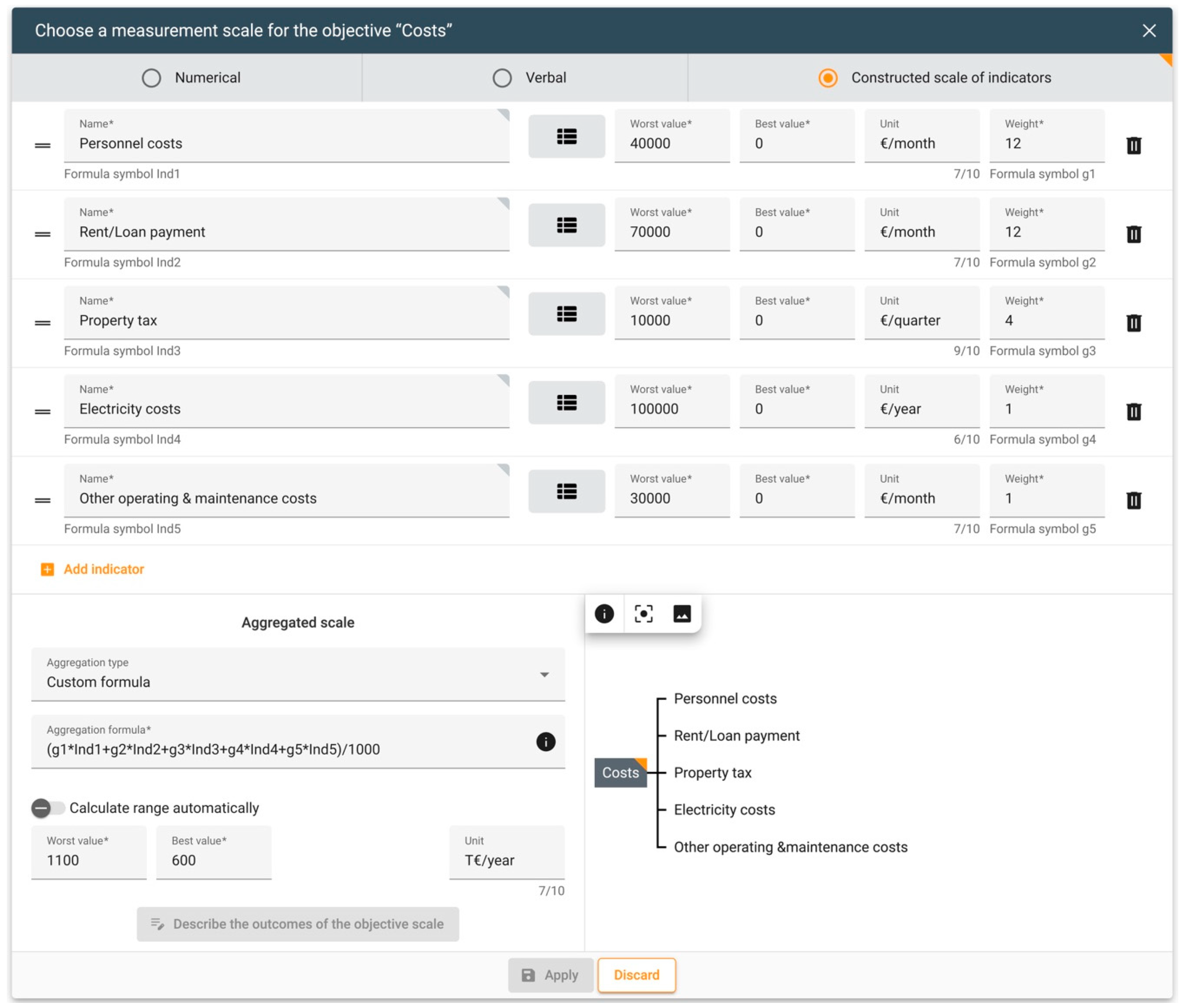Figure 2 shows the input mask for the definition of the indicator scale for the objective Costs in the Entscheidungsnavi.

Figure 2. Indicator scale for the objective Costs in the Entscheidungsnavi.

Each indicator is measured on an individual scale. Some of the costs are incurred monthly, while others are incurred quarterly or annually; e.g., Personnel costs (Ind1) are measured from 40,000 €/month (worst value) to 0 €/month (best value). Indicator weights are chosen so that we obtain the total yearly costs for all types of costs when we multiply the costs by their indicator weights; i.e., monthly costs have an indicator weight of 12, quarterly costs an indicator weight of 4, and yearly costs an indicator weight of 1. The aggregated measurement scale for costs ranges from 1100 T€/year (worst value) to 600 T€/year (best value), with the indicators being aggregated in the following way:

$$\frac{(g_{1}Ind1+g_{2}Ind2+g_{3}Ind3+g_{4}Ind4+g_{5}Ind5)}{1000}$$

5. Modeling Uncertainties in the Entscheidungsnavi

There are two categories of uncertainties to consider in MAUT. On the one hand, there are potentially uncertain forecasts about the environmental circumstances, i.e., Forecast Uncertainties (FUs) with their corresponding probabilities. On the other hand, there may be fuzziness regarding certain parameters when DMs cannot precisely specify them. This is called Parameter Uncertainty (PU) and can occur, e.g., for utilities, objective weights, and the probabilities of the environmental circumstances.

PU is commonly dealt with using fuzzy theory, which is particularly useful for translating verbal input into actionable numerical data. While DMs may have problems eliciting a specific probability for an event, they can commonly state that an event is very likely or unlikely. Fuzzy theory is used to assign degrees of membership to sets. In this case, a suitable membership function, e.g., of triangular, trapezoidal, or Gaussian shape, might assign a probability between 70% and 90% to the state ‘very likely’.

Even though it is possible to include fuzzy theory in the MAUT model [33] to a certain degree, the philosophical and theoretical foundations of MAUT limit the joint applicability of the two concepts, as MAUT heavily relies on the elicitation of probabilities. It is, however, still possible to account for fuzziness regarding parameters. The Entscheidungsnavi allows DMs to specify a mean and a degree of precision for parameters. This is comparable to the membership function of fuzzy set theory, as we limit the sets to the interval described by the mean and the degree of precision and assume a uniform distribution. Picking up on the previous example, the DM would have to specify a mean probability of 80% and a degree of precision according to Formula (8a,b) to achieve a similar result. While eliciting these values is harder for the DM, it helps them reflect on the decision situation and generates more transparency.

5.1. Modeling of Forecast Uncertainties (FUs)

Often, DMs cannot easily forecast the consequences in a consequences table. This can be due to consequences being dependent on external factors out of their control, which we call FUs. A common example would be the expected level of competition at a new location, which cannot be precisely specified, having an impact on the number of customers.

To account for this kind of uncertainty, the Entscheidungsnavi allows the DM to specify an influence factor that the consequence of an alternative regarding an objective depends on: i.e., an influence factor can be used to describe the consequence of any cell in the consequences table. While it is possible to use several different influence factors for different cells, it is only possible to use a single influence factor for any cell. The Entscheidungsnavi offers the DM two kinds of influence factors to model FUs: user-defined influence factors and a predefined influence factor.

5.1.1. User-Defined Influence Factors

When the uncertainty in FUs can be attributed to (a combination of) specific external factors with specific events, the DM can model this by utilizing user-defined influence factors, where the possible events are depicted by different states of the influence factor. In the Entscheidungsnavi, this is implemented by assigning probabilities to the states $P\left(s_{ij}^k\right)$ (see Formula (1)) of every influence factor $\widehat{\mathbb{S}}$, from which the DM can choose a set $\mathbb{S}$ to use for their decision. These influence factors can either be individual influence factors ${\widehat{\mathbb{S}}}_{ind}\subset \widehat{\mathbb{S}}$ or combined influence factors ${\widehat{\mathbb{S}}}_{com}\subset \widehat{\mathbb{S}}$. Together with $S_{cer}\in \widehat{\mathbb{S}}$, an influence factor with one state and 100% probability to model certainty, they encompass the entire set of influence factors ${\widehat{\mathbb{S}}}_{ind}\cup {\widehat{\mathbb{S}}}_{com}\cup \left\{S_{cer}\right\}=\widehat{\mathbb{S}}$. Individual influence factors (${\widehat{\mathbb{S}}}_{ind}$) are the simpler form for modeling uncertainties, where the DM specifically defines all the different states and the probability with which they occur. Combined influence factors (${\widehat{\mathbb{S}}}_{com}$) are comparatively more complex, as they are a combination of two previously defined influence factors, for which the probabilities are calculated automatically. They can be used by the DM to model FUs when the consequence depends on multiple external factors.

We let $S_{\alpha }, S_{\beta }\in \widehat{\mathbb{S}}$ denote (combined) influence factors without a connection to a consequence; i.e., $S_{\alpha }$, $S_{\beta }$ can be any $S_{ij}$ if the DM chooses to assess the consequence of objective $O_i$ for alternative $A_j$ using this influence factor. The DM can combine any $S_{\alpha }$ and $S_{\beta }$ that have not yet been set in a relationship with one another either directly or indirectly through some previously defined combined influence factor(s). For two influence factors $S_{\alpha },S_{\beta }$ with $K_{\alpha }$ and $K_{\beta }$ different states, the resulting newly defined combined influence factor $S_{\gamma }\in {\widehat{\mathbb{S}}}_{com}$ has $K_{\gamma }=K_{\alpha }\times K_{\beta }$ different states. The state probabilities of the combined influence factor for the case where the $d$-th state of influence factor $S_{\alpha }$ and the $e$-th state of influence factor $S_{\beta }$ occur simultaneously are denoted by $P\left(s_{\gamma }^{de}\right)$. Consequently, they are determined by multiplying the state probabilities $P\left(s_{\alpha }^d\right)$ and $P\left(s_{\beta }^e\right)$ of the individual influence factors that make up the state of the combined influence factor (see Formula (4)).

$$P\left(s_{\gamma }^{de}\right)=P\left(s_{\alpha }^d\right)\times P\left(s_{\beta }^e\right)$$

(4)

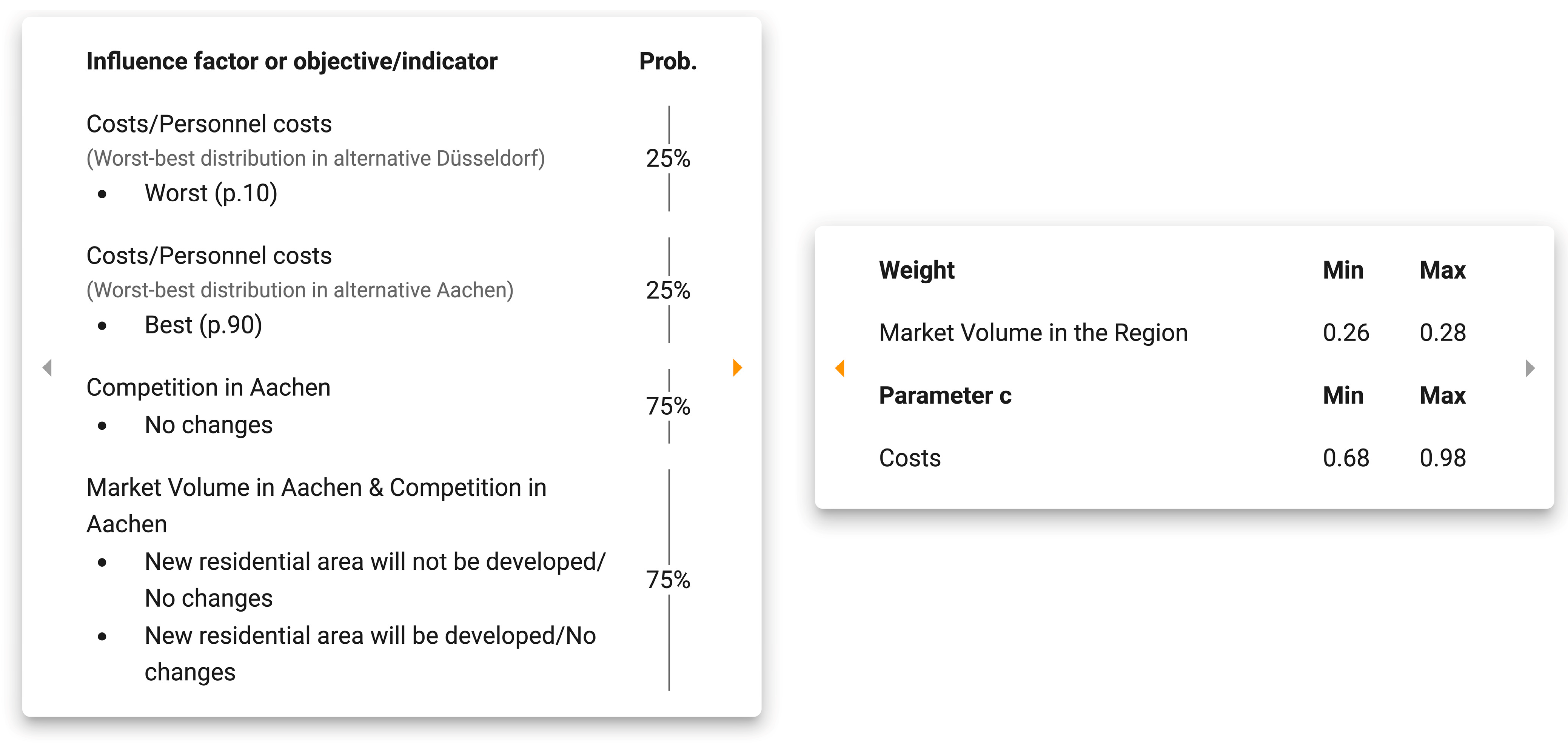
In the case study, 258 GmbH defines three individual influence factors and one combined influence factor to model the FUs of their decision (see Figure 3). The individual influence factor Shortage of Skilled Workers in Oelde is used to assess the consequence for the cell Oelde/Market Volume in the Region. Oelde is located in a very rural area, which is becoming less and less attractive to young people, which leads to problems in recruiting apprentices. Due to the limited attractiveness, only a few people move to Oelde from outside the area. In combination, these two factors indicate that a shortage of skilled workers will be expected in the future. The influence factor comprises two states with the following probabilities: No shortage of skilled workers (60%) and a Shortage of skilled workers (40%). Therefore, the company defines the consequence for each state, resulting in a range of consequences for the cell Oelde/Market Volume in the Region in the consequences table (see Figure 1). The combined influence factor merges the two individual influence factors Market Volume in Aachen and Competition in Aachen.

Figure 3. Influence factors in the Entscheidungsnavi.

If necessary, the company can add more states to its influence factors. Moreover, they can choose to base the probabilities on an automatic preset, where they can adjust the probabilities by defining the expected value and dispersion of the distribution. If the given probabilities do not add up to 100%, as required by Formula (1b), the Entscheidungsnavi normalizes the probabilities. Additionally, as the company is unsure about the exact probabilities, it has used PUs by defining a ‘precision interval’ for the influence factor Shortage of Skilled Workers in Oelde. PUs will be discussed in more detail in Section 5.2.

5.1.2. Predefined Influence Factor

If the uncertainty regarding the consequences of a cell in the consequences table cannot be attributed to one or a few specific external factors, the DM can model this type of uncertainty by using a predefined influence factor with a ‘worst-median-best’ distribution. This is often necessary when the uncertainty stems from using a large amount of data from previous or external projects to determine the likely consequences. Predefined influence factors require the p.10, p.50, and p.90 quantiles for the consequences to be specified. Using probabilities of 25% for p.10 and p.90 and 50% for p.50 is a good approximation of a normal distribution [34].

Contrary to the probability distributions of user-defined influence factors, the probability distributions for the predefined influence factor are stochastically independent. This is necessary due to the lack of specific external factors that cause the uncertainty, which can be different for every cell of the consequences table. If the consequence in a cell is assessed through multiple indicators (see Section 4, Figure 2), this stochastic independence even applies to the consequences of the individual indicators; e.g., while personnel costs could take their best value, the rent might take the median value.

In the case study, 258 GmbH cannot specify the exact costs that would result from choosing the individual alternatives and, therefore, uses the predefined influence factor to assess the consequences for the objective Costs for all alternatives. This allows the company to specify the consequences independently for each quantile and indicator, resulting in a range of consequences for each alternative. For example, the consequences range from 1037.34 T€/year to 1082 T€/year for the alternative Cologne (see Section 3, Figure 1).

5.2. Modeling of Parameter Uncertainties (PUs)

It is also common for DMs to have trouble specifying the exact parameters of a decision model; i.e., PU exists. In these cases, it is important to enable DMs to work with this uncertainty and allow imprecise information to be entered. In the Entscheidungsnavi, PUs can occur for three different types of parameters: the utilities $U_i$, the objective weights $w_i$, and the probability distributions $P\left(S_{ij}\right)$ of the influence factors. The idea of PUs in the Entscheidungsnavi for all three types of parameters is to identify a mean $\mu$ and a degree of precision $\epsilon$, resulting in an interval for the parameters. If the DM defines $\epsilon =0$, they can precisely elicit the parameter, whereas $\epsilon >0$ means that they use imprecise information. The handling of imprecise information is different for each type of parameter and will subsequently be explained.

5.2.1. PU Regarding Utilities

The way in which utilities are determined depends on the scale of the respective objective, which can be either a verbal or a numerical scale. The latter also includes indicator scales. The utility for verbal scales is determined with the help of discrete utilities, as shown in Formula (2a). The utilities for numerical scales are determined by using the exponential utility function shown in Formula (2b). For a deeper explanation of how utilities are determined in the Entscheidungsnavi, see von Nitzsch et al. [12].

When PU regarding discrete utilities is present, the utility $U_i\left(x_{ij}^k\right)$ of the consequence $x_{ij}^k$ is determined according to a continuous uniform distribution $U$ between the minimum $U_i^{min}\left(x_{ij}^k\right)$ and maximum $U_i^{max}\left(x_{ij}^k\right)$ utilities of the consequence, i.e., $U_i\left(x_{ij}^k\right) ~ U\left(U_i^{min}\left(x_{ij}^k\right),U_i^{max}\left(x_{ij}^k\right)\right).$ The minimum and maximum utilities are calculated according to Formula (5a,b) using the degree of precision ${\epsilon }_{U_i}>0$ for a discrete utility scale of the objective $O_i$, which can range from 0 to 50%.

$$U_i^{min}\left(x_{ij}^k\right)=U_i\left(x_{ij}^k\right)-{\epsilon }_{U_i}min\left\{U_i\left(x_{ij}^k\right),\right. \left.1-U_i\left(x_{ij}^k\right)\right\}$$

(5a)

$$U_i^{max}\left(x_{ij}^k\right)=U_i\left(x_{ij}^k\right)+{\epsilon }_{U_i}min\left\{U_i\left(x_{ij}^k\right),\right. \left.1-U_i\left(x_{ij}^k\right)\right\}$$

(5b)

For numerical scales, the utility $U_i\left(x_{ij}^k\right)$ of the consequence $x_{ij}^k$ is determined according to Formula (2b) using $c_i~ U\left(c_i^{min},c_i^{max}\right)$, where ${\epsilon }_{c_i}$ (between 0 and 10) is the degree of precision for a numerical utility function, and the minimum risk aversion parameter $c_i^{min}$ and maximum risk aversion parameter $c_i^{max}$ for objective $O_i$ are determined according to Formula (6a,b).

$$c_i^{min}=c_i-{\epsilon }_{c_i}$$

(6a)

$$c_i^{max}=c_i+{\epsilon }_{c_i}$$

(6b)

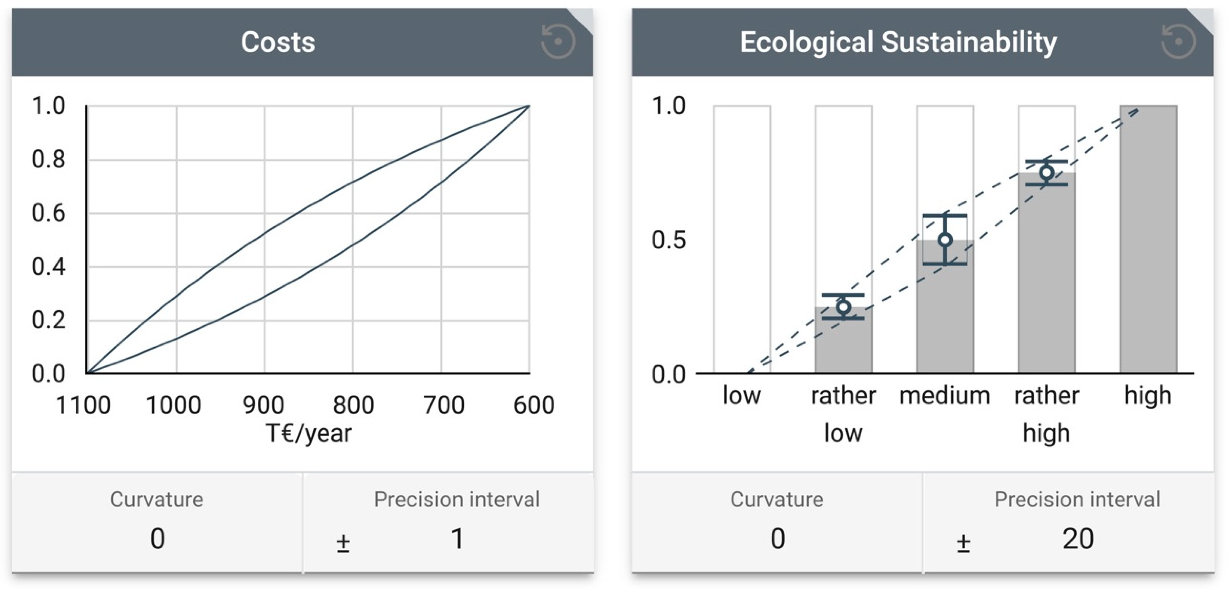
In the case study, 258 GmbH chooses linear utility functions and a linear increase in the discrete utilities for all objectives. However, the company defines precision intervals for the objectives Costs and Ecological Sustainability since it is unsure about its (risk) preferences for these objectives. Figure 4 shows an overview of the utility determination for the objectives Costs and Ecological Sustainability. For the objectives Costs, 258 GmbH chooses a precision interval of one, leading to a set of possible utility functions. This means that all utility functions within this set reflect the company’s preferences. For the objective Ecological Sustainability, 258 GmbH chooses a precision interval of 20. This also means that the utility of the individual levels is not precisely defined but lies within an interval. In both cases, the worst and best levels are determined by exact values: zero and one.

Figure 4. The determination of utility functions for the objectives Costs and Ecological Sustainability in the Entscheidungsnavi.

5.2.2. PU Regarding Objective Weights

The objective weights $w_i$ are determined by eliciting the exchange rates between two objectives through the trade-off method. Therefore, the DM has to choose a reference objective with which all other objectives are compared and then formulate preference statements for all pairs of objectives (trade-offs). The Entscheidungsnavi supports the DM by visualizing the trade-offs through indifference curves. If the DM chooses to use imprecise information for the objective weights, the individual objective weights $w_i$ are determined within their lower bounds $w_i^{min}$ and upper bounds $w_i^{max}$ according to a continuous uniform distribution $w_i~ U\left(w_i^{min},w_i^{max}\right)$. The bounds $w_i^{min}$ and $w_i^{max}$ are determined according to Formula (7a,b) using the degree of precision ${\epsilon }_{w_i}$ for every objective $O_i$. As having imprecise objective weights usually results in the sum of all objective weights deviating from 1, it is necessary to normalize them according to Formula (7c). In this case, the normalized objective weights $w_i^{normalized}$ replace $w_i$ in the calculation of the expected utility from Formulas (1) and (1b).

$$w_i^{min}=w_i-{\epsilon }_{w_i}$$

(7a)

$$w_i^{max}=w_i+{\epsilon }_{w_i}$$

(7b)

$$w_i^{normalized}=\frac{w_i}{\sum _{v=1}^I{w}_v}$$

(7c)

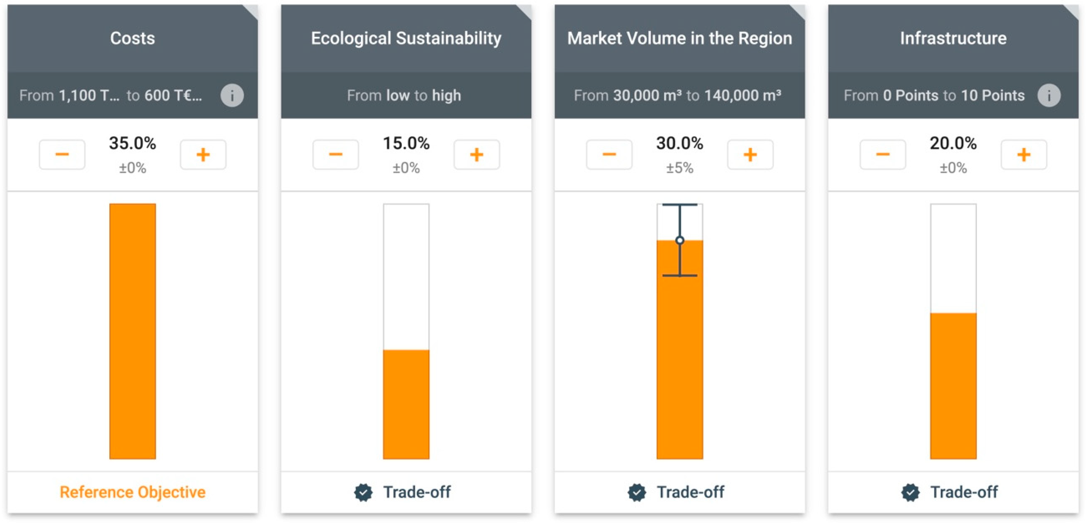
Figure 5 shows an overview of the determination of the objective weights in the Entscheidungsnavi. 258 GmbH chooses Costs as the reference objective, with which every other objective is compared in a trade-off. Every trade-off can be analyzed in detail. Figure 6 shows the detailed trade-off view of the objectives Costs and Market Volume in the Region. In this case, the company chooses a precision interval of ${\epsilon }_{w_{Market}}=5\%$, which leads to an interval from 25% to 35% for this objective weight.

Figure 5. Overview of determination of objective weights in the Entscheidungsnavi.

Figure 6. Detailed view of determination of trade-off between Costs and Market Volume in the Region in Entscheidungsnavi.

The detailed view (see Figure 6) shows the indifference curves (left side) resulting from the imprecise trade-off (right side). The company has chosen Cologne as a reference point for the trade-off with which two other imaginary alternatives (comparison points) are compared.

5.2.3. PU Regarding Probability Distributions

In cases where the DM cannot precisely elicit the state probabilities for an individual influence factor $S_{\delta }\in {\widehat{\mathbb{S}}}_{ind}$, they can define a degree of precision $0\le {\epsilon }_{P\left(S_{\delta }\right)}\le 50\%$ for this influence factor. This means that we have to find a probability distribution $P^{norm}\left(S_{\delta }\right)$ where the sum of all probabilities $\sum _{f=1}^{K_{\delta }}{P}^{norm}\left(s_{\delta }^f\right)$ equals one, and the probabilities $P^{norm}\left(s_{\delta }^f\right)$ of all $1\le f\le K_{\delta }$ states are between their minimum probability $P_{min}\left(s_{\delta }^f\right)$ and maximum probability $P_{max}\left(s_{\delta }^f\right)$ according to the given degree of precision. The minimum and maximum probabilities of the individual states are determined according to Formula (8a,b).

$$P_{min}\left(s_{\delta }^f\right)=P\left(s_{\delta }^f\right)-{\epsilon }_{P\left(S_{\delta }\right)}min\left\{P\left(s_{\delta }^f\right),\right. \left.1-P\left(s_{\delta }^f\right)\right\}$$

(8a)

$$P_{max}\left(s_{\delta }^f\right)=P\left(s_{\delta }^f\right)+{\epsilon }_{P\left(S_{\delta }\right)}min\left\{P\left(s_{\delta }^f\right),\right. \left.1-P\left(s_{\delta }^f\right)\right\}$$

(8b)

Simply determining the probabilities according to a continuous uniform distribution between the minimum and maximum probabilities will most likely result in the sum of all probabilities deviating from one. The subsequent necessary normalization step could, however, result in probabilities that are below or above the minimum and maximum probabilities if they have been scaled naïvely according to Formula (9).

$$P^{norm}\left(s_{\delta }^f\right)=\frac{P^{norm}\left(s_{\delta }^f\right)}{\sum _{v=1}^{K_{\delta }}{P}^{norm}\left(s_{\delta }^v\right)}$$

(9)

To avoid this, we use an algorithmic approach, where the individual probabilities $P^{norm}\left(s_{\delta }^f\right)$ are drawn in ascending order, and we ascertain that the sum of all probabilities equals one. For this, we will assume that the probabilities of $S_{\delta }$ are sorted in ascending order: i.e., $S_{\delta }=\left\{s_{\delta }^1, s_{\delta }^2, \dots , s_{\delta }^{K_{\delta }}\right\}$ is partially ordered by the relation $P\left(s_{\delta }^f\right)\le P\left(s_{\delta }^{f+1}\right)$. The probabilities $P^{norm}\left(s_{\delta }^f\right)$ are uniformly drawn from the interval between a specific minimum probability $P_{min}^{norm}\left(s_{\delta }^f\right)$ and maximum probability $P_{max}^{norm}\left(s_{\delta }^f\right)$ with a given degree of precision ${\epsilon }_{P\left(S_{\delta }\right)}$.

The specific minimum probability is determined according to the recursive Formula (10a) and in a way that ensures that all subsequent probabilities will be between their respective minimum $P_{min}\left(s_{\delta }^f\right)$ and maximum $P_{max}\left(s_{\delta }^f\right)$ probabilities. At the same time, they must at least be able to account for the remaining probability to ensure the sum of all probabilities is one.

$$P_{min}^{norm}\left(s_{\delta }^f\right)=\left\{\begin{array}{cc}{P}_{min}\left(s_{\delta }^f\right)& if f=1\\ \mathit{max}\left\{P_{min}\left(s_{\delta }^f\right), 1-\sum _{g=1}^{f-1}{P}^{norm}\left(s_{\delta }^g\right)-\sum _{g=f+1}^{K_{\delta }}{P}_{max}\left(s_{\delta }^g\right)\right\}& if 1<f<K_{\delta }\\ 1-\sum _{g=1}^{K_{\delta }-1}{P}^{norm}\left(s_{\delta }^g\right)& if f=K_{\delta }\end{array}\right.$$

(10a)

The specific maximum probability is determined analogously according to Formula (10b) while ensuring that we can at least allocate the minimum probability $P_{min}\left(s_{\delta }^f\right)$ to all subsequent states.

$$P_{max}^{norm}\left(s_{\delta }^f\right)=\left\{\begin{array}{cc}{P}_{max}\left(s_{\delta }^f\right)& if f=1\\ \mathit{min}\left\{P_{max}\left(s_{\delta }^f\right), 1-\sum _{g=1}^{f-1}{P}^{norm}\left(s_{\delta }^g\right)-\sum _{g=f+1}^{K_{\delta }}{P}_{min}\left(s_{\delta }^g\right)\right\}& if 1<f<K_{\delta }\\ 1-\sum _{g=1}^{K_{\delta }-1}{P}^{norm}\left(s_{\delta }^g\right)& if f=K_{\delta }\end{array}\right.$$

(10b)

Using this, the probabilities are determined by multiplying the possible range of the probability by a random variable $rnd ~ U\left(\mathrm{0,1}\right)$ and adding this to the specific minimum probability, as in Formula (11).

$$P^{norm}\left(s_{\delta }^f\right)=P_{min}^{norm}\left(s_{\delta }^f\right)+\left(P_{max}^{norm}\left(s_{\delta }^f\right)-P_{min}^{norm}\left(s_{\delta }^f\right)\right)\ast rnd$$

(11)

In the case study, 258 GmbH is unsure about the probabilities of the states of the influence factor Shortage of Skilled Workers in Oelde. Therefore, they adjust the degree of precision to use imprecise probabilities with $\epsilon =10\%$ (see Section 5.1.1, Figure 3). This results in an interval for both states. The probability of the state No shortage of skilled workers in Oelde lies between 56% and 64%, and the probability of the state Shortage of skilled workers in Oelde lies between 36% and 44%.

6. Methods for Checking the Robustness of the Result

While including FUs and PUs can greatly increase the complexity of the decision model, it often cannot be avoided. The expected utility of the MAUT model only captures the resulting risk in a limited way, as extreme results for rare events can be concealed by the method of aggregation. The robustness check can, however, reveal these risks and serve as a good starting point to identify alternatives and uncertainties that warrant further consideration. Using a simulation approach, the tool calculates a ranking of the alternatives for randomly generated scenarios that are based on the previously defined PUs and FUs with their given probabilities. It, therefore, helps the DM check how robust the ranking of alternatives is, pointing out scenarios in which an otherwise promising alternative might fall behind.

The analysis is based on a Monte Carlo simulation [35], as even decision models that are otherwise manageable in size can easily result in an infeasible number of calculations. For example, having a decision model with five alternatives and five objectives that are each measured through five indicators, using the predefined influence factor (with three states) for all forecasts results in $3^{5\ast 5\ast 5}\approx 4.36\times {10}^{59}$ different possibilities due to stochastic independence, making it infeasible to calculate an analytically correct result, even on the fastest computer to date. The simulation approach in the Entscheidungsnavi provides a very good approximation of this result with only a few million iterations. Furthermore, the DM can select the FUs, i.e., influence factors, and PUs, i.e., uncertainties regarding probabilities, utilities, and objective weights, for which they want to check robustness. This allows for specific analyses to be carried out while also giving the option to reduce computational complexity.

Running the simulation with enabled FUs generates information on how the alternatives react to the given influence factors, i.e., external factors out of the control of the DM. In this kind of simulation, it can be interesting to examine which requirements are necessary for an alternative to be the best and how likely these requirements are to be met. To generate this information, the specific state of every individual influence factor is drawn according to the discrete probability distribution of the influence factor for every simulation iteration. The states of combined influence factors are determined by a combination of states of the individual influence factors.

By enabling PUs for the simulation, DMs gain insights into how their inability to precisely elicit certain parameters affects the result. Based on this information, the DM can consider whether they should spend more time and effort on determining the parameters of the model or not. If the model is sensitive to PU (i.e., the best alternative depends on a randomly drawn parameter within the given interval), the DM should try to give a more precise assessment to aid the overall robustness of the model. To examine the influence of PUs, the uncertain parameters of every simulation iteration are determined according to the methodology explained in Section 5.2.

It is also possible to analyze the robustness of PUs and FUs simultaneously. This generates the most substantial insights, as every kind of uncertainty is considered. Any inferences on the robustness of the outcome should generally be based on a simulation covering PUs and FUs, while analyzing only individual PUs and FUs can aid the decision-making process through the generation of specific information. When running the simulation with FUs and PUs, a specific discrete probability distribution is drawn for all selected influence factors with imprecise probabilities for every simulation iteration. These specific probability distributions are then used to draw the specific states for every influence factor, as previously described for the case where only FU occurs.

The outcome of the Monte Carlo simulation is visually presented to the DM (see Figure 7). The Entscheidungsnavi shows a tabular overview of how often each individual alternative was ranked first, second, third, etc., in the simulation iterations performed. A score is calculated from all the frequencies for every alternative, which reflects the weighted average of ranks achieved on the basis of these frequencies. The lower this score is, the more frequently an alternative is in the top ranks and the more attractive it is. This score is used to check for a new form of dominance, namely, simulation dominance. It can be regarded as similar to stochastic dominance in that it takes probabilities into account. An alternative that achieves a score of exactly one absolutely dominates all other considered alternatives according to the simulation: i.e., it is better in every single iteration of the simulation. If the score deviates from one, no strict simulation dominance exists. The score can, however, still be interpreted as the degree of dominance.

Figure 7. Robustness check of case study in Entscheidungsnavi.

When only two alternatives are considered, the score for the alternatives can lie between one and two, and their sum adds up to three. As previously mentioned, an alternative with a score of one absolutely dominates the other alternatives, while a score close to one will indicate a strong degree of dominance of one alternative over the other. A score of 1.1 indicates that the alternative is better in 90% of cases, for example. A complete lack of dominance between the alternatives is ascertained when the scores for both alternatives are 1.5, i.e., when they are both the better alternative in 50% of the cases.

The Entscheidungsnavi also collects information on which states or which combination of states is necessary for the rank of an alternative. In the case where a state occurs in all scenarios that lead to a specific rank for an alternative, this information is deemed to be a requirement for the alternative to achieve a specific rank and will be presented to the DM. Additionally, the DM is presented with the range of calculated (conditional) expected utilities for each alternative to better grasp the extent of the impact on the individual alternatives. This can be interesting in cases where a DM wants to avoid risk and opt for an alternative that may be ranked lower in the average rank but shows little deviation in the expected utility across all simulation runs.

For efficiency reasons, the simulation is stopped once the average maximum change in the frequency with which an alternative achieves a rank is below ${10}^{-7}$ per iteration over the course of one second for any alternative. This is considered a stable result that approximates an analytical result well while keeping the necessary resources to a minimum. The DM can, however, always choose to continue the simulation if they want more valid results.

In this case study, the alternative Düsseldorf ranks first in almost all simulation iterations (see Figure 7). The expected utility varies between 57.98 and 69.80 and is only surpassed by the utility of Aachen in very few constellations. Depending on the values drawn, the second- and third-placed alternatives change, too. Aachen ranks second in 57% and third in 43% of iterations. Cologne ranks second in 43% and third in 57% of iterations. Oelde ranks last in almost all iterations (99.4%) of the simulation, while in a few cases, Cologne becomes the worst alternative (0.06%). While the result shows a very strong preference for the warehouse in Düsseldorf, there is still a small risk involved where Aachen would be the best alternative. Therefore, it is reasonable to further explore the conditions under which Aachen should be chosen for the location of the warehouse.

Hovering over the frequency bar for Aachen in the first place gives 258 GmbH insights on the necessary requirements (see Figure 8) to reach this rank. The Entscheidungsnavi provides the DM with information on the necessary influence factor states, objective weights, and utilities. In this case, Aachen only becomes the best alternative through a combination of FUs and PUs. This is indicated by the necessity for the influence factors on the left and the deviations of the objective weights and risk aversion parameter $c_{costs}$ from their defined means $w_{Market vol.}=0.3$ and $c_{costs}=0$, respectively.

Figure 8. Necessary requirements for Aachen to become best alternative.

7. Objective Weight Analysis

Eliciting one’s objective weights is one of the hardest parts of the decision-making process. In many cases, DMs are uncertain about their objective weights, up to the point where they cannot even properly elicit them using precision intervals. In these cases where DMs have a high PU regarding the objective weights, the objective weight analysis can be a helpful starting point to see which objective weight intervals would result in different outcomes, i.e., a different alternative with the highest expected utility.

The objective weight analysis uses a simulation approach and determines a range of statistical measures for the different objective weights that result in an alternative being the best, namely, the minimum, maximum, p.10 and p.90 quantiles, median, and average. These are initially determined by different objective weight combinations algorithmically chosen in each calculation step. The number of increments $N_{inc}$ of the objective weights describes the granularity with which the objective weights are altered during the simulation and depends on the number of objectives $\left|\mathbb{O}\right|$. The incrementation values have been chosen to provide a good ratio between the number of necessary calculations and the granularity of the objective weights. The different increment numbers can be seen in Formula (12).

$$N_{inc}=\left\{\begin{array}{cc}1000\hfill & if \left|\mathbb{O}\right|=2\\ 100\hfill & if \left|\mathbb{O}\right|=3\\ 40\hfill & if \left|\mathbb{O}\right|=4\\ 18\hfill & if \left|\mathbb{O}\right|=5\\ 11\hfill & if \left|\mathbb{O}\right|=6\\ 8\hfill & if \left|\mathbb{O}\right|=7\\ 6\hfill & if \left|\mathbb{O}\right|=8\\ 5\hfill & if \left|\mathbb{O}\right|=9\\ 4\hfill & if 10\le \left|\mathbb{O}\right|\le 11\\ 3\hfill & if 12\le \left|\mathbb{O}\right|\le 14\\ 2\hfill & if 15\le \left|\mathbb{O}\right|\end{array}\right.$$

(12)

The number of iterations for the algorithm depends on the number of objectives and amounts to the number of increments to the power of the number of objectives, i.e., $N_{inc}^{\left|\mathbb{O}\right|}$, and ranges between 500 thousand and 4.7 million for decisions with 14 or fewer objectives. For the calculation of the objective weights, we introduce the notation $⌊z⌋$ for the greatest integer less than or equal to z. Furthermore, we use the binary operation $y mod z$, as used in computer science [36], which returns the remainder of the division $\frac{y}{z}$ for any real numbers $y$ and $z$ (13a).

$$y mod z=y-z⌊\frac{y}{z}⌋,\hspace{1em}\hspace{1em}where z\ne 0;y mod 0=y; y,z\in \mathbb{Z}$$

(13a)

With this, we calculate the objective weight for objective $O_i$ in iteration $\lambda$ of the algorithm according to Formula (13b).

$$w_i^{\lambda }=\left(⌊\frac{\lambda }{N_{inc}^{i-1}}⌋ mod N_{inc}\right)\frac{1}{N_{inc}-1},\hspace{1em}\hspace{1em}where 1\le i\le \left|\mathbb{O}\right|, 1\le \lambda \le N_{inc}^{\left|\mathbb{O}\right|}$$

(13b)

To generate all possible objective weight combinations with the number of increments, we need a function that iterates through the different incremental values for the different objectives. The term $⌊\frac{\lambda }{N_{inc}^{i-1}}⌋$ delays the incrementation of $\lambda$ by a factor equal to the number of increments from one objective $w_i$ to another objective weight $w_{i+1}$; i.e., the function will repeat the same value for $N_{inc}^{i-1}$ times before increasing the value by one. Furthermore, the $mod$ function helps us ensure that we always have as many different integer results as we have increments: i.e., for an input value that is a multiple of the increments, the result will be zero, while the results are between one and the number of increments minus one for all other input values. In combination, this allows us to iterate through every possible objective weight combination regarding the number of increments. We can then multiply this value by $\frac{1}{N_{inc}-1}$ to generate equidistant unnormalized objective weights between zero and one.

If, at the end of the algorithm, the change in any of the statistical values recorded is greater than 0.05% for the calculations during the last ½ second of the algorithm, the Entscheidungsnavi will continue the simulation with randomly generated objectives weights $w_i^{\lambda }~U[0,1]$ until the maximum change in any of the values for all calculations during ½ second is less than 0.05%. Either way, the normalized objective weights $w_i^{\lambda ,norm}$ will be determined for every objective $i$ and every iteration $\lambda$ according to Formula (14) to obtain a valid set of objective weights for every iteration of the algorithm.

$$w_i^{\lambda ,normalized}=\frac{w_i^{\lambda }}{\sum _{v=1}^I{w}_v^{\lambda }}$$

(14)

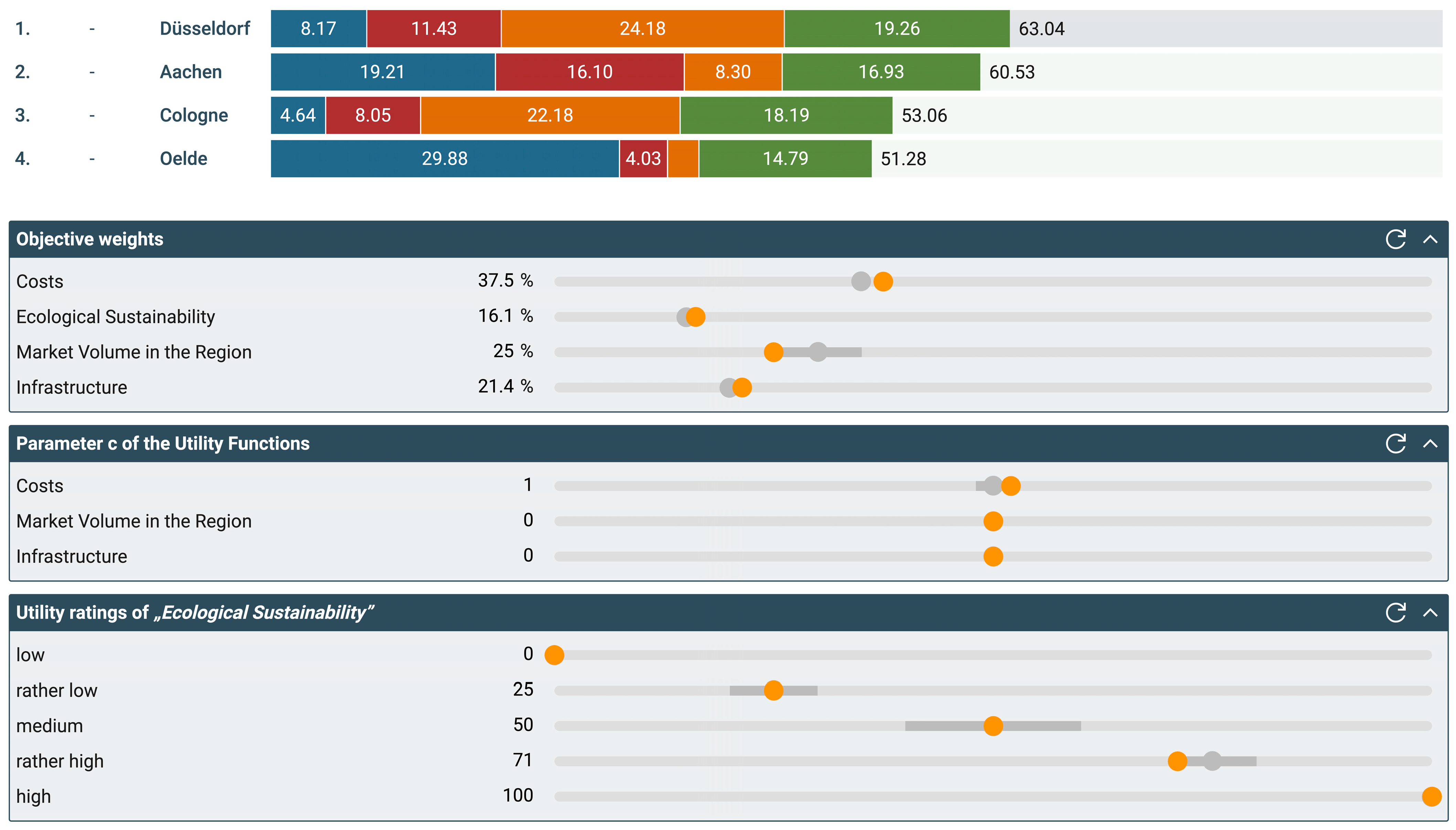
Figure 9 shows the objective weight analysis in the Entscheidungsnavi based on the case study. On the left, the DM can see how often an alternative has ended up in first place across all simulation runs. By default, the alternatives that most frequently reached first place are at the top. In the bar chart in the middle, the DM can see the average objective weights of the entire simulation for which the alternatives were the best (display: average) and the range of objective weights that can occur while an alternative is the best. In the more detailed view (display: distribution), the DM can also see the medians, the maximum and minimum values, and the p.10 and p.90 quantiles of the drawn objective weights with which the corresponding alternative has ended up in first place. The DM can also change the quantiles in this view to p.25 and p.75 quantiles.

Figure 9. Objective weight analysis in the Entscheidungsnavi.

The objective weight analysis (Figure 9) further strengthens the robustness of the result with Düsseldorf as the warehouse’s location. Even with objective weights outside the specified uncertainty, it is still the most promising location in 68.74% of cases. Only objective weights of 61% and above for Costs and above 71.7% for Ecological Sustainability hinder Düsseldorf from being in first place. However, in 27.55% of cases, Aachen becomes the best alternative when varying the objective weights. The narrow interval of possible objective weights for Market Volume in the Region can be attributed to Aachen’s relative weakness in that regard. The upper limit of 28.07% is, however, still within the uncertainty interval defined by 258 GmbH for this objective. Therefore, further analysis should be conducted.

Above the bar chart, DMs can also select which alternatives should be displayed. In addition, they can change the sorting based on their gut feeling. With the button on the top right, DMs can choose to vertically enlarge the diagram. When the DM hovers over the bars, the exact values of the different parameters are shown (see Figure 9).

8. Sensitivity Analysis

The sensitivity analysis helps DMs to check the plausibility of the model, i.e., whether the different parameters have the expected impact on the result and how big the impact is. This is mainly enabled by the multidimensional approach of the Entscheidungsnavi. While most other tools only allow a unidimensional analysis of the changes caused by varying a parameter, the Entscheidungsnavi offers the option to vary all parameters simultaneously. This allows the DM to analyze the impact of multiple uncertainties at the same time, which gives more realistic results than changing just one value at a time.

The sensitivity analysis allows the variation in the following parameters of the decision model: objective weights, utilities, probabilities of FUs, consequences, and indicator weights. Corresponding slider boxes are available for each parameter. The effects on the resulting ranking and utilities of alternatives can be observed while changing the slider. It is also possible to select which alternatives are shown.

The detailed display option for expected utilities shows the utility broken down into the contribution of each objective. Hovering over the colored bars shows the DM which objective the shown utility belongs to. All values are multiplied by 100 for better readability.

If imprecise parameters have been chosen, the precision interval specified by the DM is marked graphically on the slider with a dark-gray area. The DM can use this to easily check whether there are any effects on the result within the previously defined intervals.

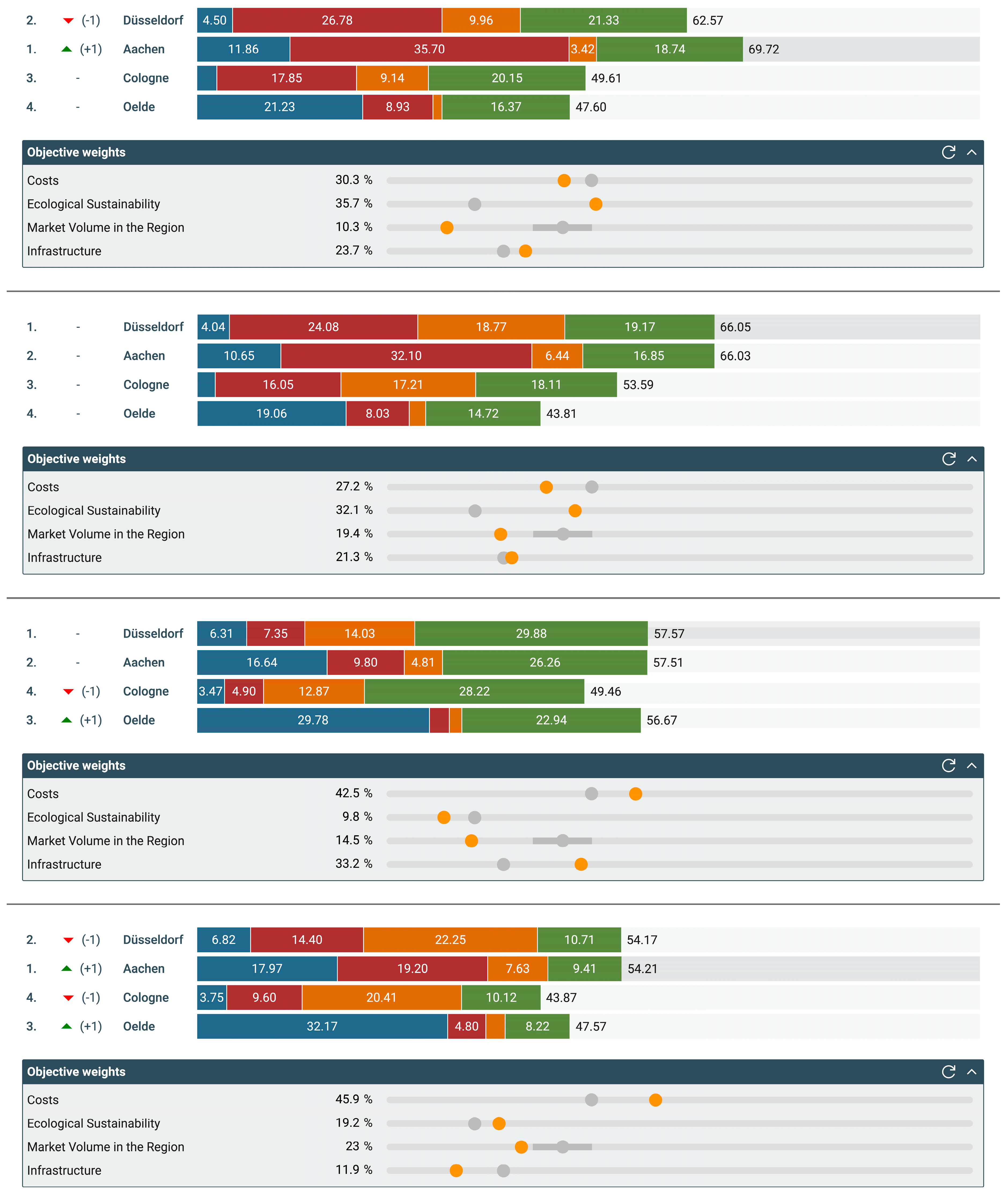
In the case study, 258 GmbH can use the sensitivity analysis to analyze the risks previously identified in the robustness check and objective weight analysis. Figure 10 shows the analysis regarding PU and confirms the findings indicated by the simulation of the robustness check. Even when all PUs take the least favorable values for Düsseldorf in accordance with the defined uncertainty intervals for the respective parameters, it still remains on top. 258 GmbH has minimized the objective weight for Market Volume in the Region (orange bar), where Düsseldorf has a higher utility than Aachen. It has also maximized the risk aversion parameter $c_{Costs}$, benefiting Aachen’s utility value, as the concave utility function generates a higher utility increase for Aachen than it does for Cologne as if the utility function were linear. Lastly, it has minimized the utility value for the rather high consequence level of the objective Ecological Sustainability, which is the consequence for Düsseldorf. As changing the PUs is not sufficient to put Aachen in first place, it can be said that the choice of location must also depend on the FUs identified in the robustness check (Figure 8), i.e., costs associated with the warehouses at the locations, the level of competition, and market volume in Aachen. Knowing this, 258 GmbH could try to perform a more precise assessment of the probabilities or the costs to minimize the effect of uncertainty on the model or use other types of analyses to assure themselves that they are making the right choice.

Figure 10. Sensitivity analysis for PU impact.

Figure 11 shows the continued analysis, this time regarding the risks from the objective weight analysis. Even though they were only uncertain about the exact objective weight of Market Volume in the Region, it is still reasonable to ensure that the result is maximally robust in this regard. Using the average objective weights that put Aachen in first place in the objective weight analysis, they conducted an extended investigation into possible thresholds that change the result. The starting point shows a considerable lead in utility for the location in Aachen but also a high deviation from the elicited objective weights for Ecological Sustainability and Market Volume in the Region, pointing to a strength in the first and a weakness in the latter for Aachen. Gradually increasing the objective weight for Market Volume in the Region shows that upon reaching an objective weight of 19.4%, Düsseldorf becomes the best alternative yet again. The same happens at 9.8% when decreasing the objective weight for Ecological Sustainability. A third analysis shows that even when trying to deviate as little as possible from the original objective weights, there is still a major deviation necessary to put Aachen in first place.

Figure 11. Sensitivity analysis for the impact of objective weights with detailed utilities for the objectives Costs (blue), Ecological Sustainability (red), Market Volume in the Region (orange), and Infrastructure (green).

9. Indicator Impacts, Tornado Diagrams, and Risk Profiles

There are three ways to visualize uncertainties and their associated risks in the Entscheidungsnavi: indicator impacts, tornado diagrams, and risk profiles.

9.1. Indicator Impacts

Indicator scales are helpful in assessing consequences because they give DMs a more granular form of input. When they are combined with influence factors, the Entscheidungsnavi can visualize the impact of the uncertainty for individual indicators on the overall consequence of an objective. Therefore, using indicator scales also makes it easier for DMs to gain insights into the main contributing factors for the consequences in a matrix cell and their associated risks. This can inform DMs for which uncertainties it would be most beneficial to gather more exact predictions and for which uncertainties the increased effort might be too costly.

The indicator impact diagram is available for every cell of the consequences table where an indicator scale is utilized. The diagram clearly shows which indicators have the greatest, the second greatest, etc., impact on the outcome for such a cell based on the respective existing FU. Depending on the type of influence factor used, i.e., user-defined or predefined, the DM is presented with different information and has different options to modify the diagram.

When the predefined influence factor is used, the impact of the indicators is initially determined under the assumption that either the Worst, Median, or Best state occurs for the indicator for which the impact is being determined, and the Median state occurs for all other indicators (selection: simple variant). The DM can, however, choose to have the impact determined under the assumption that either the Worst, Median, or Best state occurs for the indicator for which the impact is being determined and the states of all other indicators occur with a frequency according to their defined probability distributions (selection: probabilistic variant). To generate the information regarding the indicator impacts for user-defined influence factors, we treat the indicators as if their states were stochastically independent, even though they are not, and always calculate their impacts according to the probabilistic variant.

Figure 12 shows the indicator impacts on the objective Costs for the alternative Cologne in the Entscheidungsnavi. 258 GmbH can choose between three different display options for the range of the results scale: total scale (the entire bandwidth of the scale is used as a basis), worst–best scenarios (the limit of the scale results from a combination of the indicated best or worst results of the indicators), and adjusted (the range adjusts to the actual width of the indicator impact diagram). Moreover, the indicators can be sorted by their influence on the result or in the order in which the DM defined them.

Figure 12. Indicator impacts for the objective Costs in the alternative Cologne in the Entscheidungsnavi.

In this case study, the indicator Personnel costs has the biggest impact on the result of the objective Costs in the alternative Cologne, followed by the indicators Other operating & maintenance costs and Electricity costs. The indicator Other operating & maintenance costs causes the result to vary between 1063 T€/year and 1055 T€/year. Hovering over the bars will show these values to the DM.

9.2. Tornado Diagrams

Similarly to indicator impact diagrams, tornado diagrams present the DM with information about the impact of uncertainties on the utility, however, on a larger scale. They show the resulting change in expected utility for an alternative based on certain events occurring, i.e., conditional expected utilities. These effects can be analyzed in isolation when choosing a single alternative or in comparison to another alternative. This comparison is particularly interesting if the decision is to be made between two alternatives. In such a case, the DM can clearly see under which circumstances one alternative is better and for which uncertainties. The influence factor with the greatest impact and, therefore, the widest bar is shown at the top, and the other influence factors follow in descending order of impact. This also sheds light on which uncertainties should preferably be analyzed further, e.g., through more precise probability estimates, if the DM wants to reduce uncertainty in the decision situation.

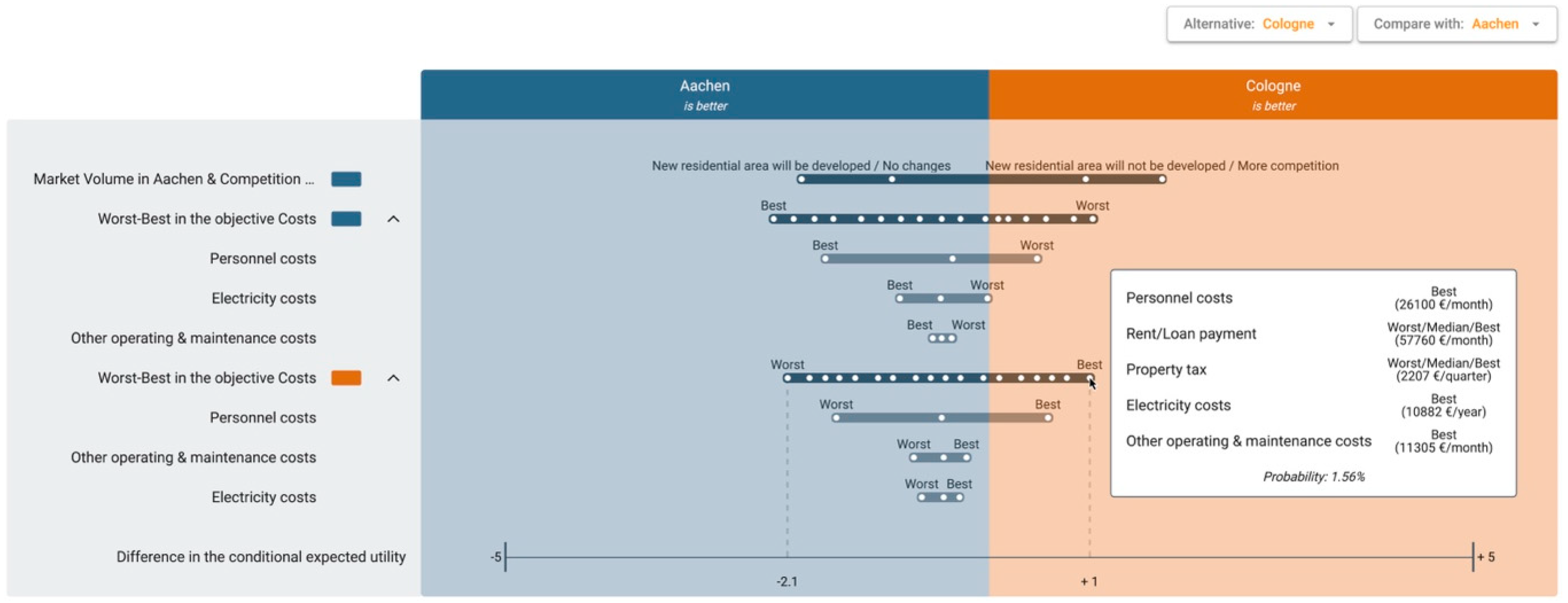
Figure 13 shows a comparison of two alternatives, Cologne and Aachen, in the tornado diagram. It helps the DM reflect how the uncertainties from the defined influence factors affect the evaluation of the alternatives.

Figure 13. Tornado diagram for overall result in Entscheidungsnavi.

If an objective is assessed through multiple indicators and the assessment is based on the predefined influence factor, DMs can expand the influence factor on the left and see the isolated effects of uncertainty on the individual indicators.

In the case study, 258 GmbH selects a compared alternative (Cologne) on the top right (see Figure 13). It is evident in the comparison of the two alternatives that uncertainties have the greatest impact on the relative advantage. Colored rectangles next to the influence factor names indicate which alternative the uncertainty refers to. Here, the combined influence factor ‘Market Volume in Aachen & Competition in Aachen’ has the greatest impact on the difference in the conditional expected utility, which varies between −1.9 and +1.8. Furthermore, 258 GmbH has the option to analyze the impact of the predefined influence factor in more depth. For the objective Costs, the conditional expected utility ranges between −2.1 and +1.0 because of the worst–best influence factor. By hovering over the individual points, DMs can see which indicator states lead to a certain conditional expected utility and how likely they are. With this illustration, the company can clearly see which states of the influence factor occur for the indicators when an alternative is better.

9.3. Risk Analysis

The Entscheidungsnavi offers multiple ways to analyze the risk associated with choosing an alternative. This analysis can be either conducted individually for every objective or aggregated over all objectives. When considering all objectives, it is also possible to analyze risk with and without the DM’s preferences and objective weights.

9.3.1. Individual Risk Profiles and Stochastic Dominance

Risk profiles can be considered a tool for experts with profound knowledge in decision theory. They show the likeliness of exceeding results and can, therefore, be used to check for dominance. In some cases, this can help DMs eliminate alternatives from consideration to reduce the complexity of the model and, therefore, efficiently use the resources available.

A risk profile $R\left(x\right)$ shows the probability of exceeding a certain result $x$. This means that $R\left(x\right)$ has a complementary relation to the distribution function $F\left(x\right)$, i.e., $R\left(x\right)=1-F\left(x\right)$. The DM can generate a risk profile for each cell in the consequences table, i.e., $R_{ij}\left(x_i\right)$ with ${x_i^{-}\le x}_i\le x_i^{+}$, for an alternative regarding a single objective that is determined using the distribution function for the specific influence factor $S_{ij}$. Based on this, comparisons can be made with other alternatives regarding the same objective, and first-degree stochastic dominance (for this context, see Hadar & Russell [37]) can thus be determined graphically for a single objective.

This type of dominance check is also conducted automatically, simultaneously over all objectives on a mathematical basis once the assessments of alternatives in the objectives have been completed. This is referred to as the dominance of alternative $\xi$ over $\pi$ if $\xi$ stochastically dominates $\pi$ in all objectives, i.e., if the risk profile for alternative $\xi$ is identical to or above that of alternative $\pi$ and above it for at least one point (see Formula (15)). Neither utility functions nor objective weights need to be defined for this.

$$\begin{gathered} R_{i\xi }\left(x_i\right)\ge R_{i\pi }\left(x_i\right) | 1\le i\le \left|\mathbb{O}\right|,\forall x_i\in \left[x_i^{-},x_i^{+}\right] \\ with at least one strong inequality for one i_0,x_0 \end{gathered}$$

(15)

Alternatives that are dominated by another alternative are marked in red with an info button. Clicking on this info button shows which alternative(s) dominate(s) the one in question. DMs can use this information to carefully consider whether or not to further analyze alternatives that are stochastically dominated for all objectives. Even if an alternative is dominated, it can still be the best alternative in rare scenarios. If an alternative is dominated by multiple alternatives or an alternative for which the assessment depends on the same influence factors, DMs can likely exclude it from further analysis.

In the case study, the alternative Düsseldorf dominates the alternative Cologne, as shown by the red marking in Figure 14. However, Düsseldorf only stochastically dominates Cologne over all objectives. While Cologne also achieves better outcomes than the other two alternatives for most objectives, Aachen and Oelde achieve better outcomes than Düsseldorf for Ecological Sustainability and Costs, respectively.

Figure 14. Checks for stochastic dominance in the Entscheidungsnavi.

9.3.2. Risk Comparison

DMs can also analyze the risk associated with the alternatives on the basis of their preference statements regarding utilities and objective weights. The risk comparison shows the overall utilities of the alternatives, i.e., $R_j^{overall}\left(\omega \right)$, with $0\le \omega \le 1$, aggregated across all objectives. The x-axis then shows the possible utilities of the alternatives, each of which only results under the condition that certain overall forecast scenarios occur. In this representation, the utility functions used are, strictly speaking, no longer interpreted as utility functions but as value functions. For the difference between these two functions, see Dyer and Sarin [38,39]. The information shown in the diagram is generated via a Monte Carlo simulation. The underlying data are equivalent to those generated in the robustness check when only FUs, i.e., influence factors, are considered.

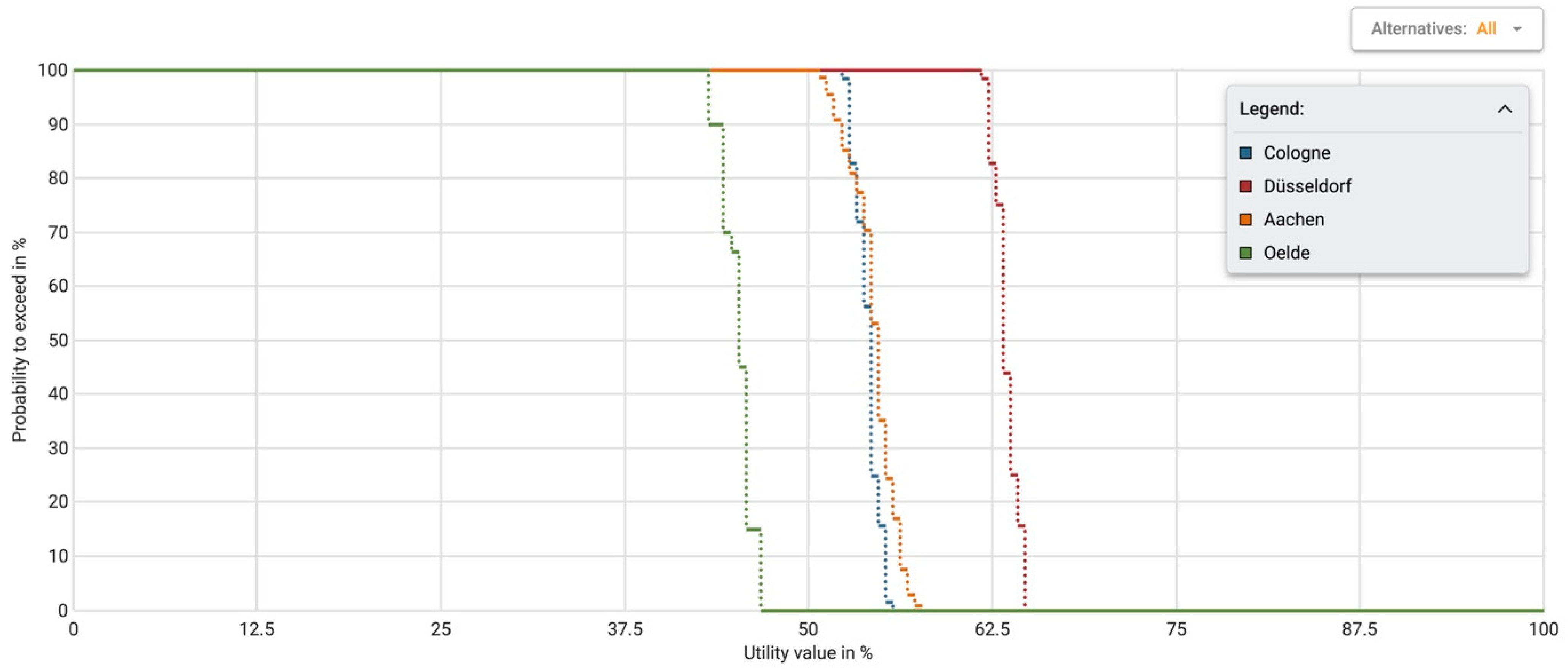
Figure 15 shows the risk comparison for the case study. It confirms the previous finding that opening the wood warehouse in Düsseldorf is a good choice, as it further confirms the previous finding regarding the alternative’s robustness. By analyzing the diagram, 258 GmbH can see that Düsseldorf can be regarded as the best alternative when looking at the likeliness of attaining an overall utility level, as it has the highest probability of all alternatives of exceeding any given utility.

Figure 15. Risk comparison in the Entscheidungsnavi.

10. Conclusions

This paper shows how uncertainties are integrated into a multi-criteria decision analysis in the DSS Entscheidungsnavi and how the methods and analyses can help support the desired reflection of the DM. Therefore, different types of uncertainties are described, and various methods are explained to analyze these uncertainties. The basic mathematical model in the system is the additive utility function of MAUT, which allows two types of uncertainties: Forecast Uncertainties (FUs) and Parameter Uncertainties (PUs). FUs can be modeled by influence factors in the consequences table. In the Entscheidungsnavi, a distinction is made between user-defined and predefined influence factors. User-defined influence factors can either be individual or combined influence factors. The predefined influence factor is based on a ‘worst-median-best’ distribution. PUs can be used if DMs cannot precisely determine the parameters of a decision model and only imprecise information is available. In the Entscheidungsnavi, PUs can be modeled for three different parameters: utility functions, objective weights, and the probabilities of the influence factors. With the help of PUs, DMs can define the intervals of these parameters. Furthermore, the paper presents various methods and analyses to check the impact of uncertainties, namely, methods for checking the robustness of the result, objective weight analysis, sensitivity analysis, and indicator impacts, tornado diagrams, risk profiles.

In the robustness check, a Monte Carlo simulation is used to check how robust the result is regarding FUs and PUs. This analysis gives DMs a better insight into how stable the ranking of the alternatives is regarding previously determined uncertainties. The objective weight analysis can be used as a starting point to see which objective weight intervals would result in a different ranking of alternatives. In the sensitivity analysis, DMs can analyze which parameters impact the result of the decision and to what degree. It is possible to vary the following parameters: objective weights, utilities, probabilities of FU, consequences, and indicator weights. Indicator impacts, tornado diagrams, and risk profiles help DMs visualize risks in the decision model. With the help of checks for stochastic and simulation dominance, DMs can identify dominated alternatives without determining utilities or objective weights.

The limitations of the proposed mathematical model under MAUT shown in this paper are the general applicability of the additive model and the use of expected utilities according to von Neumann and Morgenstern [26]. We assume (and demand) that the objectives of the decision situations are fundamental, measurable, redundancy-free, complete, and preference-independent. Other limitations are of a technical nature with regard to the possible and necessary number of iterations in the Monte Carlo simulation to reach a satisfactory validity of the results. In the case of the objective weight analysis, this is counteracted by gradually decreasing the granularity with which the objective weights are altered with an increasing number of objectives. Furthermore, due to the high development speed of browser engines and their supported technology, the Entscheidungsnavi officially only supports the last three major browser versions for the most common browsers, i.e., Firefox, Chrome, Safari, and Edge. While it will mostly run on older browsers as well, some functionalities might be limited or missing, as the tool often relies on new browser functions to support the best user experience possible.

In the future, further functionalities will be added to the Entscheidungsnavi. For example, it should soon be possible to use correlated combined influence factors to display FUs in the consequences table. Furthermore, a team version is currently being developed in which it will be possible to work with several team members on a decision situation and analyze it. The uncertainties in such a team decision result from the different preferences and information bases of the individual team members. It is important to create transparency here so that a considered decision can be made in the interests of all team members.