An In-Depth Investigation of the Riemann Zeta Function Using Infinite Numbers

Abstract

This study focuses on an in-depth investigation of the Riemann zeta function. For this purpose, infinite numbers and rotational infinite numbers, which have been introduced in previous studies published by the author, are used. These numbers are a powerful tool for solving problems involving infinity that are otherwise difficult to solve. Infinite numbers are a superset of complex numbers and can be either complex numbers or some quantification of infinity. The Riemann zeta function can be written as a sum of three rotational infinite numbers, each of which represents infinity. Using these infinite numbers and their properties, a correlation of the non-trivial zeros of the Riemann zeta function with each other is revealed and proven. In addition, an interesting relation between the Euler–Mascheroni constant (γ) and the non-trivial zeros of the Riemann zeta function is proven. Based on this analysis, complex series limits are calculated and important conclusions about the Riemann zeta function are drawn. It turns out that when we have non-trivial zeros of the Riemann zeta function, the corresponding Dirichlet series increases linearly, in contrast to the other cases where this series also includes a fluctuating term. The above theoretical results are fully verified using numerical computations. Furthermore, a new numerical method is presented for calculating the non-trivial zeros of the Riemann zeta function, which lie on the critical line. In summary, by using infinite numbers, aspects of the Riemann zeta function are explored and revealed from a different perspective; additionally, interesting mathematical relationships that are difficult or impossible to solve with other methods are easily analyzed and solved.

1. Introduction

The Riemann zeta function, denoted by the Greek letterζ (zeta), is a mathematical function of a complex variable (s) defined by the Dirichlet series (1) for Re(s) > 1, as well as its analytic continuation elsewhere, minus the point s =1. The Riemann zeta function is a meromorphic function on the whole complex plane, which is holomorphic everywhere except for a simple pole at s = 1 with residue 1. We notice that if we set s =1, we obtain the well-known harmonic series that diverts. We also notice that whenever Re(s) ≤ 1, the considered Dirichlet series also diverges. Euler was the first to give any substantial analysis of this series. The values of the Riemann zeta function at even positive integers were computed by Euler. The first of them, ζ(2), provides a solution to the famous Basel problem. In 1979, Roger Apery proved the irrationality of ζ(3). The values at negative integer points, also found by Euler, are rational numbers and play an important role in the theory of modular forms. The Riemann zeta function plays a pivotal role in analytic number theory and has applications in probability theory, physics, and statistics. In a sense, the Riemann zeta function is a magical tool that has propelled math and physics forward and threaded together many disparate fields in these disciplines, even though we still do not understand it well. Zeta functions are encountered in statistical mechanics when evaluating bosonic and fermionic particle distributions. The energy values of heavy nuclei (such as uranium) are distributed like the zeros of the Riemann zeta function. This means that the quantum mechanics of heavy nuclei are connected to prime numbers, which is an incrediblestatement in itself. Due to its relation to random matrices, the zeta function also appears in the study of neural networks, image processing, and wireless communications. It is unbelievable how much knowledge has been produced by the zeta function.

$$\zeta (s)={\displaystyle \sum _{\mathrm{n}=1}^{\infty }\frac{1}{{\mathrm{n}}^s}}$$

(1)

Euler’s most important contribution to the theory of the zeta function is the Euler product formula (2). This formula explicitly demonstrates the connection between prime numbers and the zeta function. The Euler product formula is also called the analytic form of the fundamental theorem of arithmetic. It demonstrates how the Riemann zeta function encodes information on the prime factorization of integers and the distribution of primes. The Euler product formula can be used to calculate the asymptotic probability that (s) randomly selected integers are set-wise coprime. Intuitively, the probability that any single number is divisible by a prime (or any integer) p is 1/p. Hence, the probability that s numbers are all divisible by this prime is 1/p^s, and the probability that at least one of them is not is (1 − 1/p^s).

$$\zeta (s)={\displaystyle \sum _{\mathrm{n}=1}^{\infty }\frac{1}{{\mathrm{n}}^{\mathrm{s}}}}={\displaystyle \prod _p{\left(1-\frac{1}{p^s}\right)}^{-1}}$$

(2)

The Riemann hypothesis is usually stated as follows: all the non-trivial zeros of the Riemann zeta function lie on the line Re(s) = 1/2 (critical line) of the complex plane. This hypothesis makes a very precise connection between two seemingly unrelated mathematical objects (namely, prime numbers and the zeros of analytic functions). Its solution will give us profound insight into number theory and, in particular, the nature of prime numbers. The great mathematician David Hilbert is credited with the following phrase “If I were to awaken after having slept for a thousand years, my first question would be: Has the Riemann hypothesis been proven?” [1].

The functional Equation (3) was also established by Riemann in his famous 1859 paper “On the Number of Primes Less Than a Given Magnitude” [2] and was used to construct the analytic continuation in the first place. The functional equation shows that the Riemann zeta function has zeros at −2, −4, −6, …; these are called the trivial zeros. They are trivial in the sense that their existence is relatively easy to prove; for example, from sin(πs/2) being 0 in the functional equation [3,4,5,6,7,8,9,10,11,12,13,14,15,16,17,18,19,20,21,22,23,24,25,26,27,28,29,30,31,32,33,34,35,36,37].

$$\zeta (s)=2^s{\pi }^{s-1}\sin \left({\displaystyle \frac{\pi s}{2}}\right)\Gamma (1-s)\zeta (1-s)$$

(3)

The quantification of infinity is a reasonable search for the human mind, dating back to the 19th century. The idea of quantitative infinity started from works by Cantor, Gottlob Frege, and Richard Dedekind [38,39,40,41,42,43] and continued after the mid-20th century with nonstandard analysis, which was developed by Abraham Robinson [44,45,46,47,48,49,50]. In the author’s previous papers—[51,52,53,54]—new infinite numbers and rotational infinite numbers were introduced with their properties and calculations. Unlike previous attempts, these infinite numbers quantify infinity in a way that is different from past efforts (by applying the theory of limits of functions) and are a useful tool for solving problems where infinity appears. The set of infinite numbers is a superset of the complex number set.

Using these numbers and functions, the extended (in the set of infinite numbers) Laplace and bilateral Laplace transforms, also proposed in [51,53], make it possible to solve specific differential equations defined piecewise over the entire domain of real numbers (−∞, +∞). Moreover, by using infinite number functions, a long series of infinite terms can be nicely transformed into a short, elegant infinite number function whose computation is an easy task. In general, infinite numbers are useful in solving mathematical and natural science problems where infinity occurs, such as series of infinite terms, improper integrals, limits of the form ∞/∞ in cases where we cannot use L’Hospital’s rule, etc., since infinite numbers offer the possibility of arithmetic operations and calculations.

This study presents a novel approach to investigating the Riemann zeta function. A new mathematical framework is introduced to analyze the non-trivial zeros of the Riemann zeta function, using infinite numbers and rotational infinite numbers. First, correlations of the non-trivial zeros of the Riemann zeta function with each other, as well as with the Euler–Mascheroni constant, are revealed and proven. Based on these correlations, interesting limits involving series and sequences of numbers with the non-trivial zeros of the Riemann zeta function are easily proven. In addition, a numerical verification of the results is presented. Finally, a new method for the numerical calculation of the zeros of the Riemann zeta function lying on the critical line is demonstrated. Interesting diagrams that better illustrate the results are presented. In conclusion, based on the above, the use of ordinary/rotational infinite numbers, with their properties, can easily provide an in-depth investigation of the Riemann zeta function, revealing interesting relations and solving problems that are quite difficult or impossible to solve using conventional methods. Such problems, for example, include those described below by relations (10), (29), (30), (38), and (43). The study integrates both theoretical and numerical methods to validate its claims and provides extensive mathematical derivations and graphical representations to support the findings. The application of infinite numbers as a tool to study the Riemann zeta function is innovative and provides a fresh perspective on an extensively researched problem.

The rest of this study is organized as follows: Section 2 presents some preliminary concepts and formulas regarding infinite numbers. Section 3 reveals and proves correlations of the Riemann zeta function non-trivial zeros with each other, as well as with the Euler–Mascheroni constant. In Section 4, a numerical validation is presented where the previously demonstrated results are verified numerically. Section 5 presents a new numerical method for calculating the zeros of the Riemann zeta function lying on the critical line. In Section 6, the conclusions of this study are presented.

2. Preliminary Concepts

As shown in [51,52,53], relation (4) defines the infinity unit (ξ). Moreover, every single-value, continuous, differentiable, and non-oscillating complex function, φ(·), of the infinity unit, ξ, namely, the function φ(ξ), is an “infinite number function”, which is also an “infinite number”. Furthermore, “rotational infinite functions” were defined as the functions of the infinity unit, ξ, of the form A(ξ)e^iφ(ξ), where A(ξ) and φ(ξ) are ordinary infinite numbers/functions. These “rotational infinite functions” are also “rotational infinite numbers”. They represent not single numbers but sets of infinite numbers [54].

$$\xi \equiv \underset{x\to +\infty }{\lim }(x)\mathrm{where}x\in ℝ$$

(4)

An infinite number can be represented in the complex plane by a vector, whose measure is equal to the measure of the infinite number, and its angle (with respect to the positive real axis) is equal to the angle of this infinite number. Rotational infinite numbers are generated as the ordinary infinite numbers are rotated in the complex plane. The important property of ordinary infinite numbers and rotational infinite numbers is that they make possible calculations with infinity that are otherwise impossible. The reason for this is that the infinity unit (ξ) no longer represents infinity in its general concept (∞) but rather its specific univocal form, as defined in Equation (4). Therefore, arithmetic operations on infinite numbers are performed just like arithmetic operations on limits of functions (as seen in the following example), since infinite numbers are basically limits of functions. However, infinite numbers/functions have additional interesting properties. One can calculate derivatives, indefinite/definite integrals, or the Laplace transform of these infinite functions. Moreover, series of infinite numbers can be equivalently transformed into simple infinite numbers/functions where calculations become an easy task.

Example 1.

Find the value of the following infinite number A:

$$\begin{array}{l}A=\left[{\displaystyle \frac{(2-i3e^{\xi })e^{i{\pi }^2}}{e^{\xi -i(2\pi +1)}}}-3\sin {(\pi +1)}^2\right]\\ =(2-i3e^{\xi })e^{i{\pi }^2}{e}^{i(2\pi +1)}{e}^{-\xi }-3\sin {(\pi +1)}^2=(2-i3e^{\xi })e^{i{(\pi +1)}^2}{e}^{-\xi }-3\sin {(\pi +1)}^2=2e^{i{(\pi +1)}^2}{e}^{-\xi }-i3e^{\xi }{e}^{i{(\pi +1)}^2}{e}^{-\xi }-3\sin {(\pi +1)}^2\\ =-i3e^{i{(\pi +1)}^2}-3\sin {(\pi +1)}^2=-i3\cos {(\pi +1)}^2+3\sin {(\pi +1)}^2-3\sin {(\pi +1)}^2=-i3\cos {(\pi +1)}^2=-i0.37691\mathrm{\dots }\end{array}$$

Infinite numbers are a superset of complex numbers. In the above example, the result of arithmetic operations is an imaginary number, namely A = −i0.37691…; therefore, infinite numbers also include complex/real numbers. However, in their generality, they constitute a broader set of numbers; for example, the number (A + 3ξ) = 3ξ − i0.37691… represents infinity and not a finite complex number. Also, the number (A +4ξ) represents infinity; however, (A + 3ξ) and (A + 4ξ) are different infinite numbers, and their difference is (−ξ).

In order to make the present article self-contained and to enable the reader to more easily follow the development of the article’s arguments,

Table 1. Basic definitions and properties of ordinary and rotational infinite numbers.

	Basic Definitions and Properties of Ordinary Infinite Numbers	Basic Definitions and Properties of Rotational Infinite Numbers
Unit:	$\xi =\underset{x\to +\infty }{\lim }(x)$, where x$\in$ℝ.	$Ru=e^{i\xi }=\underset{x\to +\infty }{\lim }{e}^{ix}$, where x$\in$ℝ.
Ordinary and rotational infinite number functions:	φ (ξ), where φ(·) is a single-value, continuous, differentiable, and non-oscillating complex function. Therefore:$\varphi (\xi )=\underset{x\to +\infty }{\lim }\varphi (x)$, where x $\in$ℝ.	A(ξ)eiφ(ξ), where A(ξ) and φ(ξ) are ordinary infinite numbers/functions. Notice that A(·)eiφ(·) is a multi-value, oscillating complex function.
Infinite number functions are also infinite numbers:	Ordinary infinite numbers.	Rotational infinite numbers.
The main differencebetween ordinary and rotational infinite numbers:	They are single numbers that can be real numbers, complex numbers, or infinity in any quantified form. Therefore, infinite numbers are a superset of complex numbers.	They are sets of ordinary infinite numbers.
Arithmetic operations (sum/subtraction/product/ratio) of two infinite numbers, ${\varphi }_1(\xi )$ and ${\varphi }_2(\xi )$:	${\varphi }_1(\xi )\pm {\varphi }_2(\xi )=\underset{x\to +\infty }{\lim }\left({\varphi }_1(x)\pm {\varphi }_2(x)\right)$ ${\varphi }_1(\xi )\cdot {\varphi }_2(\xi )=\underset{x\to +\infty }{\lim }\left({\varphi }_1(x)\cdot {\varphi }_2(x)\right)$ ${\displaystyle \frac{{\varphi }_1(\xi )}{{\varphi }_2(\xi )}}=\underset{x\to +\infty }{\lim }{\displaystyle \frac{{\varphi }_1(x)}{{\varphi }_2(x)}}$ where x $\in$ℝ.	It applies the same as with ordinary infinite numbers.
Unlike infinity in its general consideration (∞), where ∞−∞ = undefined and ∞/∞ = undefined, it applies:	ξ − ξ = 0 and ξ/ξ = 1	$e^{i\xi }-e^{i\xi }=0$ and $e^{i\xi }/e^{i\xi }=1$
Commutative and associative laws for addition and multiplication:	They apply.	Also, they apply.
Three main arguments of infinite numbers (measure, angle, velocity)	They apply.	Also, they apply.
Measure of an infinite numberwritten in the form$\varphi (\xi )=f_1(\xi )+i{f}_2(\xi )$:	$|\varphi (\xi )|=\sqrt{{f_1}^2(\xi )+{f_2}^2(\xi )}$	Also, the same applies.
Angle (θ) of an infinite number written in the form$\varphi (\xi )=f_1(\xi )+i{f}_2(\xi )$:	$\theta =\arctan \left({\displaystyle \frac{f_2(\xi )}{f_1(\xi )}}\right)$	Also, the same applies.
Velocity (v) of an infinite numberwritten in the form$\varphi (\xi )=f_1(\xi )+i{f}_2(\xi )$:	$v={\displaystyle \frac{d\varphi (\xi )}{d\xi }}={\displaystyle \frac{d{f}_1(\xi )}{d\xi }}+i{\displaystyle \frac{d{f}_2(\xi )}{d\xi }}$	Also, the same applies.
The measure of the corresponding unit:	ξ	1
The angle of the corresponding unit:	0	ξ
Velocity of the corresponding unit:	1	$e^{i\left(\xi +{\displaystyle \frac{\pi }{2}}\right)}$
The measure of the velocity of the corresponding unit:	1	1
Representation in the complex plane	They are represented by constant vectors	They are represented by rotating vectors
The inverse number of an infinite number φ(ξ), which is defined as [1/φ(ξ)]:	The inverse number of any ordinary infinite number representing infinity is zero.	Also, they exist.
Mirror number of an infinite number φ(ξ), which is defined as φ(1/ξ):	The mirror number of any ordinary infinite number representing infinity can be a finite number, zero, or infinity.	Also, they exist.
The inverse number of the corresponding unit:	1/ξ = 0	$1/e^{i\xi }=e^{-i\xi }$ (it has the same measure as the rotational infinity unit, but it rotates in the reverse direction in the complex plane).
Mirror number of the corresponding unit:	1/ξ = 0	$e^{i{\displaystyle \frac{1}{\xi }}}=e^0=1$
Angular velocity (ω) of a rotational number A(ξ)eiφ(ξ), which is defined as$\omega ={\displaystyle \frac{d\theta (\xi )}{d\xi }}$:	It is zero (ordinary infinite numbers do not rotate).	It can be a finite (not zero) real number or any infinite number being infinity.
Angular velocity(ω) of the corresponding unit:	0	1
The derivative/integral of an infinite number function, φ(ξ), is calculated if one obtains the derivative/integral of φ(x), where x$\in$ℝ, and then one takes the limit for x tending to infinity:	${\varphi }^{\prime }(\xi )=\underset{x\to +\infty }{\lim }{\varphi }^{\prime }(x)$ ${\displaystyle \int \varphi (\xi )}d\xi =\underset{x\to +\infty }{\lim }{\displaystyle \int \varphi (x)}dx$	Similarly to ordinary infinite numbers.
Since infinity is quantified via infinite numbers, the Laplace transform of any real function f(t), t $\in$ℝ, can be extended and calculated over the entire frequency spectrum (also for values of s$\in$, for which the corresponding generalized integraldoes not converge):	$F(s,\xi )={\displaystyle \underset{t=1/\xi }{\overset{t=\xi }{\int }}f(t)e^{-st}dt}$ where t $\in$ℝ and s$\in$.	Also, it applies.
The bilateral Laplace transform is also extended inthe set of infinite numbers:	$F(s,\xi )={\displaystyle \underset{t=-\xi }{\overset{t=\xi }{\int }}f(t)e^{-st}dt}$ where t $\in$ℝ and s$\in$.	Also, it applies.
Extended Laplace transforms in the set of infinite numbers, can solve specific differential equations defined piecewise over the entire domain of real numbers, also for t < 0 where the usual Laplace transform is not defined:	It applies.	Also, it applies.
Every series of infinite terms can be written equivalently as a simple infinite number. This helps to calculate difficult numerical limits.	Ιt applies.	Also, it applies.

briefly presents the basic definitions and properties of ordinary and rotational infinite numbers. In this way, the several concepts and properties of infinite numbers, which have been introduced, demonstrated, and proven in the previously published papers mentioned in the References, are presented concisely and in correspondence between ordinary and rotational infinite numbers.

It is known that the Riemann zeta function can be expressed using relation (5) (where s = α + ib and α, b, x$\in$ℝ), for values 0 <α = Re(s) < 1. As proved in detail in [54], for 0 < α <1, ζ(s) can be written as a sum of three rotational infinite numbers—A₁(ξ), A₂(ξ), and A₃(ξ) (all representing infinity)—the sum of which is a finite number C. More specifically, Equations (6)–(9) apply.

$$\zeta (\mathrm{s})={\displaystyle \frac{\mathrm{s}}{\mathrm{s}-1}}-s{\displaystyle \underset{x=1}{\overset{\infty }{\int }}\frac{x-⌊x⌋}{x^{s+1}}}dx$$

(5)

$$\zeta (\mathrm{s})=A_1(\xi )+A_2(\xi )+A_3(\xi )=C$$

(6)

$$A_1(\xi )=A_1={\displaystyle \frac{s}{s-1}}{\xi }^{-\mathrm{s}+1}$$

(7)

$$A_2(\xi )=1^{-s}+2^{-s}+3^{-s}+\mathrm{\dots }+{\xi }^{-s}$$

(8)

$$A_3(\xi )=-\xi \cdot {(\xi +1)}^{-\mathrm{s}}=-{\displaystyle \frac{\xi }{{(\xi +1)}^{\mathrm{s}}}}=-{\displaystyle \frac{{\xi }^s}{{(\xi +1)}^{\mathrm{s}}}}\cdot {\displaystyle \frac{\xi }{{\xi }^s}}=-{\left({\displaystyle \frac{\xi }{\xi +1}}\right)}^s\cdot {\xi }^{1-s}=-{\left({\displaystyle \frac{1}{1+\raisebox{1ex}{$1$}\!\left/ \!\raisebox{-1ex}{$\xi $}\right.}}\right)}^s\cdot {\xi }^{1-s}=-{\xi }^{-s+1}$$

(9)

3. Correlation of the Non-Trivial Zeros (for α = 1/2)of the Riemann Zeta Function with Each Other and with the Euler–Mascheroni Constant

Theorem 1.

Let us consider two roots (non-trivial zeros), s₁ = α + ib₁ and s₂ = α + ib₂(α, b₁, b₂$\in$ ℝ and 0 < α < 1), of the Riemann zeta function. Then, the following relation (10) is true:

$$\underset{n\to +\infty }{\lim }{\displaystyle \frac{\frac{1}{1^a{2}^a}\cos \left(b_1\ln \frac{1}{2}\right)+\mathrm{\dots }+\frac{1}{1^a{\xi }^a}\cos \left(b_1\ln \frac{1}{n}\right)+\mathrm{\dots }+\frac{1}{{(n-1)}^a{n}^a}\cos \left(b_1\ln \frac{(n-1)}{n}\right)}{\frac{1}{1^a{2}^a}\cos \left(b_2\ln \frac{1}{2}\right)+\mathrm{\dots }+\frac{1}{1^a{\xi }^a}\cos \left(b_2\ln \frac{1}{n}\right)+\mathrm{\dots }+\frac{1}{{(n-1)}^a{n}^a}\cos \left(b_2\ln \frac{(n-1)}{n}\right)}}={\displaystyle \frac{{(\alpha -1)}^2+{b_2}^2}{{(\alpha -1)}^2+{b_1}^2}}$$

(10)

Proof. 

Previous Equation (8) is transformed into the following:

$$A_2(\xi )=1^{-a-ib}+2^{-a-ib}+3^{-a-ib}+\mathrm{\dots }+{\xi }^{-a-ib}$$

$$={\displaystyle \frac{1}{1^a}}\cdot e^{-ib\ln 1}+{\displaystyle \frac{1}{2^a}}\cdot e^{-ib\ln 2}+{\displaystyle \frac{1}{3^a}}\cdot e^{-ib\ln 3}+\mathrm{\dots }+{\displaystyle \frac{1}{{\xi }^a}}\cdot e^{-ib\ln \xi }$$

which implies the following:

$$\begin{gathered} A_2(\xi )={\displaystyle \frac{1}{1^a}}(\cos (b\ln 1)-i\sin (b\ln 1))+{\displaystyle \frac{1}{2^a}}(\cos (b\ln 2)-i\sin (b\ln 2))+{\displaystyle \frac{1}{3^a}}(\cos (b\ln 3)-i\sin (b\ln 3))+\mathrm{\dots }+{\displaystyle \frac{1}{{\xi }^a}}(\cos (b\ln \xi )-i\sin (b\ln \xi )) \\ =\left({\displaystyle \frac{1}{1^a}}\cos (b\ln 1)+{\displaystyle \frac{1}{2^a}}\cos (b\ln 2)+{\displaystyle \frac{1}{3^a}}\cos (b\ln 3)+\mathrm{\dots }+{\displaystyle \frac{1}{{\xi }^a}}\cos (b\ln \xi )\right)-i\left({\displaystyle \frac{1}{1^a}}\sin (b\ln 1)+{\displaystyle \frac{1}{2^a}}\sin (b\ln 2)+{\displaystyle \frac{1}{3^a}}\sin (b\ln 3)+\mathrm{\dots }+{\displaystyle \frac{1}{{\xi }^a}}\sin (b\ln \xi )\right) \end{gathered}$$

which further implies the following:

$${\left|A_2(\xi )\right|}^2={\left({\displaystyle \frac{1}{1^a}}\cos \left(b\ln 1\right)+{\displaystyle \frac{1}{2^a}}\cos \left(b\ln 2\right)+\mathrm{\dots }+{\displaystyle \frac{1}{{\xi }^a}}\cos \left(b\ln \xi \right)\right)}^2+{\left({\displaystyle \frac{1}{1^a}}\sin \left(b\ln 1\right)+{\displaystyle \frac{1}{2^a}}\sin \left(b\ln 2\right)+\mathrm{\dots }+{\displaystyle \frac{1}{{\xi }^a}}\sin \left(b\ln \xi \right)\right)}^2$$

(11)

or equivalently:

$$\underset{n\to +\infty }{\lim }{\left|A_2(n)\right|}^2=\underset{n\to +\infty }{\lim }{\left({\displaystyle \frac{1}{1^a}}\cos \left(b\ln 1\right)+{\displaystyle \frac{1}{2^a}}\cos \left(b\ln 2\right)+\mathrm{\dots }+{\displaystyle \frac{1}{n^a}}\cos \left(b\ln n\right)\right)}^2+{\left({\displaystyle \frac{1}{1^a}}\sin \left(b\ln 1\right)+{\displaystyle \frac{1}{2^a}}\sin \left(b\ln 2\right)+\mathrm{\dots }+{\displaystyle \frac{1}{n^a}}\sin \left(b\ln n\right)\right)}^2$$

(12)

From Equation (11), we can calculate the square of the measure of the rotational infinite number A₂(ξ) as follows:

$${\left|A_2(\xi )\right|}^2=\left({\displaystyle \frac{1}{1^{2a}}}+{\displaystyle \frac{1}{2^{2a}}}+\mathrm{\dots }+{\displaystyle \frac{1}{{\xi }^{2a}}}\right)+2\left({\displaystyle \frac{1}{1^a{2}^a}}\cos (b\ln 1)\cdot \cos (b\ln 2)+\mathrm{\dots }+{\displaystyle \frac{1}{1^a{\xi }^a}}\cos (b\ln 1)\cdot \cos (b\ln \xi )+\mathrm{\dots }+{\displaystyle \frac{1}{{(\xi -1)}^a{\xi }^a}}\cos (b\ln (\xi -1))\cdot \cos (b\ln \xi )\right)$$

$$+2\left({\displaystyle \frac{1}{1^a{2}^a}}\sin (b\ln 1)\cdot \sin (b\ln 2)+\mathrm{\dots }+{\displaystyle \frac{1}{1^a{\xi }^a}}\sin (b\ln 1)\cdot \sin (b\ln \xi )+\mathrm{\dots }+{\displaystyle \frac{1}{{(\xi -1)}^a{\xi }^a}}\sin (b\ln (\xi -1))\cdot \sin (b\ln \xi )\right)$$

$$=\left({\displaystyle \frac{1}{1^{2a}}}+{\displaystyle \frac{1}{2^{2a}}}+\mathrm{\dots }+{\displaystyle \frac{1}{{\xi }^{2a}}}\right)+2\left({\displaystyle \frac{1}{1^a{2}^a}}\cos \left(b\ln {\displaystyle \frac{1}{2}}\right)+\mathrm{\dots }+{\displaystyle \frac{1}{1^a{\xi }^a}}\cos \left(b\ln {\displaystyle \frac{1}{\xi }}\right)+\mathrm{\dots }+{\displaystyle \frac{1}{{(\xi -1)}^a{\xi }^a}}\cos \left(b\ln {\displaystyle \frac{(\xi -1)}{\xi }}\right)\right)$$

(13)

Therefore,

$$\left|A_2(\xi )\right|=\sqrt{\left({\displaystyle \frac{1}{1^{2a}}}+{\displaystyle \frac{1}{2^{2a}}}+\mathrm{\dots }+{\displaystyle \frac{1}{{\xi }^{2a}}}\right)+G(\xi )}$$

(14)

or equivalently:

$$\underset{n\to +\infty }{\lim }\left|A_2(n)\right|=\underset{n\to +\infty }{\lim }\sqrt{\left({\displaystyle \frac{1}{1^{2a}}}+{\displaystyle \frac{1}{2^{2a}}}+\mathrm{\dots }+{\displaystyle \frac{1}{n^{2a}}}\right)+G(n)}$$

(15)

where

$$G(\xi )=2\left({\displaystyle \frac{1}{1^a{2}^a}}\cos \left(b\ln {\displaystyle \frac{1}{2}}\right)+\mathrm{\dots }+{\displaystyle \frac{1}{1^a{\xi }^a}}\cos \left(b\ln {\displaystyle \frac{1}{\xi }}\right)+\mathrm{\dots }+{\displaystyle \frac{1}{{(\xi -1)}^a{\xi }^a}}\cos \left(b\ln {\displaystyle \frac{(\xi -1)}{\xi }}\right)\right)$$

(16)

or equivalently:

$$\underset{n\to +\infty }{\lim }G(n)=\underset{n\to +\infty }{\lim }2\left({\displaystyle \frac{1}{1^a{2}^a}}\cos \left(b\ln {\displaystyle \frac{1}{2}}\right)+\mathrm{\dots }+{\displaystyle \frac{1}{1^a{n}^a}}\cos \left(b\ln {\displaystyle \frac{1}{n}}\right)+\mathrm{\dots }+{\displaystyle \frac{1}{{(n-1)}^a{n}^a}}\cos \left(b\ln {\displaystyle \frac{(n-1)}{n}}\right)\right)$$

(17)

In order to have a solution of the Riemann zeta function, and taking into account Equation (6), Equation (18) is as follows:

$$\zeta (\mathrm{s})=A_1(\xi )+A_2(\xi )+A_3(\xi )=0$$

(18)

From this relationship, it follows that

$$\left|A_2(\xi )\right|=\left|A_1(\xi )+A_3(\xi )\right|$$

(19)

It should be noted that relation (19) is a necessary but not sufficient condition for the Riemann zeta function to have zeros. This means that if the Riemann zeta function has zeros, relation (19) holds. However, the inverse is not true; namely, if relation (19) holds, Equation (18) is not certain to be valid (i.e., it is not certain that the Riemann zeta function has zeros). Given that the infinite numbers A₁, A₂, and A₃ are vectors in the complex plane, it is possible for the measure |A₂| to be equal to the measure |A₁ + A₃| without the sum of these three vectors (A₁+ A₂ + A₃) being zero (relation (18)).

Based on Equations (7) and (9), we have the following:

$$A_1(\xi )+A_3(\xi )={\displaystyle \frac{s}{s-1}}{\xi }^{-s+1}-{\xi }^{-s+1}={\displaystyle \frac{1}{s-1}}{\xi }^{-s+1}={\displaystyle \frac{{\xi }^{-a+1}}{\sqrt{{(\alpha -1)}^2+b^2}}}{e}^{-i\mathrm{atan}{\displaystyle \frac{b}{\alpha -1}}}{e}^{-ib\ln \xi }={\displaystyle \frac{{\xi }^{-a+1}}{\sqrt{{(\alpha -1)}^2+b^2}}}{e}^{-i\left(\mathrm{atan}{\displaystyle \frac{b}{\alpha -1}}+b\ln \xi \right)}$$

(20)

Combining Equations (19) and (20), we have the following:

$$\left|A_2(\xi )\right|={\displaystyle \frac{{\xi }^{-a+1}}{\sqrt{{(\alpha -1)}^2+b^2}}}$$

(21)

Therefore, assuming that we have a solution of the Riemann zeta function, from Equations (14) and (21), we obtain relation (22) as follows:

$$\sqrt{\left({\displaystyle \frac{1}{1^{2a}}}+{\displaystyle \frac{1}{2^{2a}}}+\mathrm{\dots }+{\displaystyle \frac{1}{{\xi }^{2a}}}\right)+G(\xi )}={\displaystyle \frac{{\xi }^{-a+1}}{\sqrt{{(\alpha -1)}^2+b^2}}}$$

(22)

Consequently:

$$\left({\displaystyle \frac{1}{1^{2a}}}+{\displaystyle \frac{1}{2^{2a}}}+\mathrm{\dots }+{\displaystyle \frac{1}{{\xi }^{2a}}}\right)+G(\xi )={\displaystyle \frac{{\xi }^{-2a+2}}{{(\alpha -1)}^2+b^2}}$$

(23)

However, based on [51,53], the series in the above relation can be written as Equation (24), where C′ is a finite number.

$${\displaystyle \frac{1}{1^{2a}}}+{\displaystyle \frac{1}{2^{2a}}}+\mathrm{\dots }+{\displaystyle \frac{1}{{\xi }^{2a}}}={\displaystyle \int \frac{1}{{\xi }^{2a}}d\xi =\frac{{\xi }^{-2a+1}}{-2\alpha +1}}+C^{\prime }$$

(24)

The number C′ is a finite number and not infinity (not a number of the form C′(ξ)), since the derivative of $\left({\displaystyle \frac{{\xi }^{-2a+1}}{-2\alpha +1}}+C^{\prime }\right)$ is equal to ${\displaystyle \frac{1}{{\xi }^{2a}}}$ (last infinite term of the series), only if ${\displaystyle \frac{d{C}^{\prime }}{d\xi }}=0$, meaning that C′ is a finite number.

Therefore, from (23) and (24), we have Equation (25), as follows:

$${\displaystyle \frac{{\xi }^{-2a+1}}{-2\alpha +1}}+C^{\prime }+G(\xi )={\displaystyle \frac{{\xi }^{-2a+2}}{{(\alpha -1)}^2+b^2}}$$

(25)

Combining Equations (16) and (25), we obtain the following:

$$G(\xi )=2\left({\displaystyle \frac{1}{1^a{2}^a}}\cos \left(b\ln {\displaystyle \frac{1}{2}}\right)+\mathrm{\dots }+{\displaystyle \frac{1}{1^a{\xi }^a}}\cos \left(b\ln {\displaystyle \frac{1}{\xi }}\right)+\mathrm{\dots }+{\displaystyle \frac{1}{{(\xi -1)}^a{\xi }^a}}\cos \left(b\ln {\displaystyle \frac{(\xi -1)}{\xi }}\right)\right)={\displaystyle \frac{{\xi }^{-2a+2}}{{(\alpha -1)}^2+b^2}}-{\displaystyle \frac{{\xi }^{-2a+1}}{-2\alpha +1}}-C^{\prime }$$

(26)

or simply:

$$G(\xi )={\displaystyle \frac{{\xi }^{-2a+2}}{{(\alpha -1)}^2+b^2}}-{\displaystyle \frac{{\xi }^{-2a+1}}{-2\alpha +1}}-C^{\prime }$$

(27)

Considering now two roots s₁, s₂ of the Riemann zeta function, e.g., s₁ = α + ib₁ and s₂ = α + ib₂(where α, b₁, b₂$\in$ℝ), and according to Equation (26), the following will be true, where C’ and C are finite numbers:

$${\displaystyle \frac{G_1(\xi )}{G_2(\xi )}}={\displaystyle \frac{2\left(\frac{1}{1^a{2}^a}\cos \left(b_1\ln \frac{1}{2}\right)+\mathrm{\dots }+\frac{1}{1^a{\xi }^a}\cos \left(b_1\ln \frac{1}{\xi }\right)+\mathrm{\dots }+\frac{1}{{(\xi -1)}^a{\xi }^a}\cos \left(b_1\ln \frac{(\xi -1)}{\xi }\right)\right)}{2\left(\frac{1}{1^a{2}^a}\cos \left(b_2\ln \frac{1}{2}\right)+\mathrm{\dots }+\frac{1}{1^a{\xi }^a}\cos \left(b_2\ln \frac{1}{\xi }\right)+\mathrm{\dots }+\frac{1}{{(\xi -1)}^a{\xi }^a}\cos \left(b_2\ln \frac{(\xi -1)}{\xi }\right)\right)}}={\displaystyle \frac{\frac{{\xi }^{-2a+2}}{{(\alpha -1)}^2+{b_1}^2}-\frac{{\xi }^{-2a+1}}{-2\alpha +1}-C^{\prime }}{\frac{{\xi }^{-2a+2}}{{(\alpha -1)}^2+{b_1}^2}-\frac{{\xi }^{-2a+1}}{-2\alpha +1}-C}}$$

which implies the following:

$${\displaystyle \frac{\frac{1}{1^a{2}^a}\cos \left(b_1\ln \frac{1}{2}\right)+\mathrm{\dots }+\frac{1}{1^a{\xi }^a}\cos \left(b_1\ln \frac{1}{\xi }\right)+\mathrm{\dots }+\frac{1}{{(\xi -1)}^a{\xi }^a}\cos \left(b_1\ln \frac{(\xi -1)}{\xi }\right)}{\frac{1}{1^a{2}^a}\cos \left(b_2\ln \frac{1}{2}\right)+\mathrm{\dots }+\frac{1}{1^a{\xi }^a}\cos \left(b_2\ln \frac{1}{\xi }\right)+\mathrm{\dots }+\frac{1}{{(\xi -1)}^a{\xi }^a}\cos \left(b_2\ln \frac{(\xi -1)}{\xi }\right)}}={\displaystyle \frac{\frac{1}{{(\alpha -1)}^2+{b_1}^2}}{\frac{1}{{(\alpha -1)}^2+{b_2}^2}}}={\displaystyle \frac{{(\alpha -1)}^2+{b_2}^2}{{(\alpha -1)}^2+{b_1}^2}}$$

or equivalently:

$$\underset{n\to +\infty }{\lim }{\displaystyle \frac{\frac{1}{1^a{2}^a}\cos \left(b_1\ln \frac{1}{2}\right)+\mathrm{\dots }+\frac{1}{1^a{\xi }^a}\cos \left(b_1\ln \frac{1}{n}\right)+\mathrm{\dots }+\frac{1}{{(n-1)}^a{n}^a}\cos \left(b_1\ln \frac{(n-1)}{n}\right)}{\frac{1}{1^a{2}^a}\cos \left(b_2\ln \frac{1}{2}\right)+\mathrm{\dots }+\frac{1}{1^a{\xi }^a}\cos \left(b_2\ln \frac{1}{n}\right)+\mathrm{\dots }+\frac{1}{{(n-1)}^a{n}^a}\cos \left(b_2\ln \frac{(n-1)}{n}\right)}}={\displaystyle \frac{{(\alpha -1)}^2+{b_2}^2}{{(\alpha -1)}^2+{b_1}^2}}$$

(28)

□.

Remark 1.

Relation (28) correlates two random, non-trivial roots (s₁ = α + ib₁ and s₂ = α + ib₂) of the Riemann zeta function with one another.

Remark 2.

According to relation (17), for random values of α and b, G(n) is a fluctuating quantity as it is a sum of cosines. Therefore, as shown in Equation (15), the measure |A₂(n)| includes a monotonically increasing component (which is inside the parentheses) and a fluctuating component G(n), which consists of cosines (sum of cosines). This theoretical result will be verified numerically in Section 4.

Remark 3.

As shown in Equation (27), and given that 0<α<1, quantity G(ξ) = $\underset{n\to +\infty }{\lim }G(n)$ is plus infinity. Therefore, it is interesting to notice that formula (28) is the quotient of two series tending to infinity. Consequently, it is very difficult, if not impossible, to calculate this fraction using existing methods. On the other hand, infinite numbers and rotational infinite numbers used in this analysis address and solve the problem very easily.

Example 2.

Prove the following limit of Equation (29), where 14.134… and 21.022… are the imaginary parts of the first two numerically known non-trivial roots of the Riemann zeta function.

$$\underset{n\to +\infty }{\lim }{\displaystyle \frac{\frac{1}{\sqrt{1\cdot 2}}\cos \left((14.134\mathrm{\dots })\ln \frac{1}{2}\right)+\mathrm{\dots }+\frac{1}{\sqrt{1\cdot n}}\cos \left((14.134\mathrm{\dots })\ln \frac{1}{n}\right)+\mathrm{\dots }+\frac{1}{\sqrt{(n-1)\cdot n}}\cos \left((14.134\mathrm{\dots })\ln \frac{(n-1)}{n}\right)}{\frac{1}{\sqrt{1\cdot 2}}\cos \left((21.022\mathrm{\dots })\ln \frac{1}{2}\right)+\mathrm{\dots }+\frac{1}{\sqrt{1\cdot n}}\cos \left((21.022\mathrm{\dots })\ln \frac{1}{n}\right)+\mathrm{\dots }+\frac{1}{\sqrt{(n-1)\cdot n}}\cos \left((21.022\mathrm{\dots })\ln \frac{(n-1)}{n}\right)}}={\displaystyle \frac{1+4\cdot {(21.022\mathrm{\dots })}^2}{1+4\cdot {(14.134\mathrm{\dots })}^2}}$$

(29)

Proof. 

According to Theorem 1 (relation (28)), and considerings₁=1/2 + i14.134… and s₂=1/2 + i21.022…, which are the first two non-trivial roots of the Riemann zeta function, the following equation holds:

$$\begin{gathered} \underset{n\to +\infty }{\lim }{\displaystyle \frac{\frac{1}{\sqrt{1\cdot 2}}\cos \left((14.134\mathrm{\dots })\ln \frac{1}{2}\right)+\mathrm{\dots }+\frac{1}{\sqrt{1\cdot n}}\cos \left((14.134\mathrm{\dots })\ln \frac{1}{n}\right)+\mathrm{\dots }+\frac{1}{\sqrt{(n-1)\cdot n}}\cos \left((14.134\mathrm{\dots })\ln \frac{(n-1)}{n}\right)}{\frac{1}{\sqrt{1\cdot 2}}\cos \left((21.022\mathrm{\dots })\ln \frac{1}{2}\right)+\mathrm{\dots }+\frac{1}{\sqrt{1\cdot n}}\cos \left((21.022\mathrm{\dots })\ln \frac{1}{n}\right)+\mathrm{\dots }+\frac{1}{\sqrt{(n-1)\cdot n}}\cos \left((21.022\mathrm{\dots })\ln \frac{(n-1)}{n}\right)}}={\displaystyle \frac{1/4+{(21.022\mathrm{\dots })}^2}{1/4+{(14.134\mathrm{\dots })}^2}} \\ ={\displaystyle \frac{1+4\cdot {(21.022\mathrm{\dots })}^2}{1+4\cdot {(14.134\mathrm{\dots })}^2}} \end{gathered}$$

□.

Theorem 2.

The Euler–Mascheroni constant (γ) can be expressed as the limit of infinite summing terms given by the following relation (30), where the parameter b is the imaginary part of any of the infinite zeros of the Riemann zeta function that lie on the critical line.

$$\gamma =\underset{n\to +\infty }{\lim }\left({\displaystyle \frac{4n}{1+4b^2}}-\ln n-2\left({\displaystyle \frac{1}{\sqrt{1\cdot 2}}}\cos \left(b\ln {\displaystyle \frac{1}{2}}\right)+\mathrm{\dots }+{\displaystyle \frac{1}{\sqrt{1\cdot n}}}\cos \left(b\ln {\displaystyle \frac{1}{n}}\right)+\mathrm{\dots }+{\displaystyle \frac{1}{\sqrt{(n-1)\cdot n}}}\cos \left(b\ln {\displaystyle \frac{(n-1)}{n}}\right)\right)\right)$$

(30)

Proof. 

In fact, relation (30) is the limit of a sequence of numbers when n tends to infinity, minus a series of infinite numbers, as is shown in the following equation:

$$\gamma =\underset{n\to +\infty }{\lim }\left({\displaystyle \frac{4n}{1+4b^2}}-\ln n\right)-\underset{n\to +\infty }{\lim }\left(2\left({\displaystyle \frac{1}{\sqrt{1\cdot 2}}}\cos \left(b\ln {\displaystyle \frac{1}{2}}\right)+\mathrm{\dots }+{\displaystyle \frac{1}{\sqrt{1\cdot n}}}\cos \left(b\ln {\displaystyle \frac{1}{n}}\right)+\mathrm{\dots }+{\displaystyle \frac{1}{\sqrt{(n-1)\cdot n}}}\cos \left(b\ln {\displaystyle \frac{(n-1)}{n}}\right)\right)\right)$$

For α = 1/2 and values of b such that we have zeros of ζ(s) = 0, Equation (14) becomes Equation (31).

$$\left|A_2(\xi )\right|=\sqrt{\left({\displaystyle \frac{1}{1}}+{\displaystyle \frac{1}{2}}+\mathrm{\dots }+{\displaystyle \frac{1}{\xi }}\right)+G(\xi )}$$

(31)

As proven in [54], the harmonic series, written in infinite numbers, is also equal to (lnξ + γ), where γ is the Euler–Mascheroni constant, which is equal to γ = 0.57721… Therefore, relation (31) transforms into the following relation:

$$\left|A_2(\xi )\right|=\sqrt{\ln \xi +\mathsf{\gamma }+G(\xi )}$$

Furthermore,

$${\left|A_2(\xi )\right|}^2=\ln \xi +\mathsf{\gamma }+G(\xi ),\mathrm{where}\gamma =0.57721\dots$$

(32)

Also, for α = 1/2, Equation (21) transforms into the following:

$${\left|A_2(\xi )\right|}^2={\displaystyle \frac{\xi }{1/4+b^2}}={\displaystyle \frac{4\xi }{1+4b^2}}$$

(33)

or equivalently:

$$\underset{n\to +\infty }{\lim }{\left|A_2(n)\right|}^2=\underset{n\to +\infty }{\lim }{\displaystyle \frac{n}{1/4+b^2}}={\displaystyle \frac{4n}{1+4b^2}}$$

(34)

Combining Equations (32) and (33), we finally obtain relation (35).

$${\displaystyle \frac{4\xi }{1+4b^2}}=\ln \xi +\mathsf{\gamma }+G(\xi )\Rightarrow$$

$$G(\xi )={\displaystyle \frac{4\xi }{1+4b^2}}-\ln \xi -\mathsf{\gamma }$$

(35)

or equivalently:

$$\underset{n\to +\infty }{\lim }G(n)=\underset{n\to +\infty }{\lim }\left({\displaystyle \frac{4n}{1+4b^2}}-\ln n-\mathsf{\gamma }\right)$$

(36)

Considering Equation (16), Equation(35) is further written as follows:

$$\gamma ={\displaystyle \frac{4\xi }{1+4b^2}}-\ln \xi -2\left({\displaystyle \frac{1}{\sqrt{1\cdot 2}}}\cos \left(b\ln {\displaystyle \frac{1}{2}}\right)+\mathrm{\dots }+{\displaystyle \frac{1}{\sqrt{1\cdot \xi }}}\cos \left(b\ln {\displaystyle \frac{1}{\xi }}\right)+\mathrm{\dots }+{\displaystyle \frac{1}{\sqrt{(\xi -1)\cdot \xi }}}\cos \left(b\ln {\displaystyle \frac{(\xi -1)}{\xi }}\right)\right)$$

(37)

or equivalently:

$$\gamma =\underset{n\to +\infty }{\lim }\left({\displaystyle \frac{4n}{1+4b^2}}-\ln n-2\left({\displaystyle \frac{1}{\sqrt{1\cdot 2}}}\cos \left(b\ln {\displaystyle \frac{1}{2}}\right)+\mathrm{\dots }+{\displaystyle \frac{1}{\sqrt{1\cdot n}}}\cos \left(b\ln {\displaystyle \frac{1}{n}}\right)+\mathrm{\dots }+{\displaystyle \frac{1}{\sqrt{(n-1)\cdot n}}}\cos \left(b\ln {\displaystyle \frac{(n-1)}{n}}\right)\right)\right)$$

□.

Remark 4.

Therefore, relation (30) is true, where b is the imaginary part of a random zero of the Riemann zeta function, for α = 1/2.Namely, for each of the infinite zeros of the Riemann zeta function, which lie on the critical line, and where b is their corresponding imaginary part, relation (30) holds. This parametric relation (which is a different equation for each different zero of the Riemann zeta function) constitutes a new innovative way of defining the Euler–Mascheroni constant (γ), and it was proven by using infinite numbers.

Remark 5.

In contrast to the generality (Equation (17)), where for random values of α and b, G(n) is a fluctuating quantity (as seen before), when α = 1/2 and we have zeros of the Riemann zeta function, according to relation (36), quantity G(n) ceases to fluctuate, and it is a monotonically increasing quantity. In other words, a condition for having zeros of the Riemann zeta function when α = 1/2 is that G(n) is a monotonically increasing quantity. Moreover, based on Equation (15), the measure |A₂(n)| includes two monotonically increasing components; therefore, it is itself a monotonically increasing quantity. This is also clearly seen in the linear relationship (34). This theoretical result will be verified numerically in Section 4.

Example 3.

Prove the following limit of Equation (38), where b is the imaginary part of any of the infinite zeros of the Riemann zeta function, which lie on the critical line.

$$\underset{n\to +\infty }{\lim }{\displaystyle \frac{\frac{1}{\sqrt{1\cdot 2}}\cos \left(b\ln \frac{1}{2}\right)+\mathrm{\dots }+\frac{1}{\sqrt{1\cdot n}}\cos \left(b\ln \frac{1}{n}\right)+\mathrm{\dots }+\frac{1}{\sqrt{(n-1)\cdot n}}\cos \left(b\ln \frac{(n-1)}{n}\right)}{\frac{4n}{1+4b^2}-\left(\frac{1}{1}+\frac{1}{2}+\mathrm{\dots }+\frac{1}{n}\right)}}={\displaystyle \frac{1}{2}}$$

(38)

Proof. 

According to Theorem 2, Equation (30), or, equivalently, Equation(37) applies, which can be written as follows:

$$2\left({\displaystyle \frac{1}{\sqrt{1\cdot 2}}}\cos \left(b\ln {\displaystyle \frac{1}{2}}\right)+\mathrm{\dots }+{\displaystyle \frac{1}{\sqrt{1\cdot \xi }}}\cos \left(b\ln {\displaystyle \frac{1}{\xi }}\right)+\mathrm{\dots }+{\displaystyle \frac{1}{\sqrt{(\xi -1)\cdot \xi }}}\cos \left(b\ln {\displaystyle \frac{(\xi -1)}{\xi }}\right)\right)={\displaystyle \frac{4\xi }{1+4b^2}}-(\ln \xi +\gamma )$$

(39)

Furthermore, as proven in [54], the harmonic series is equal to (lnξ + γ); thus, relation (40) applies. Combining Equations (39) and (40), relation (41) is proven.

$$\ln \xi +\gamma ={\displaystyle \frac{1}{1}}+{\displaystyle \frac{1}{2}}+\mathrm{\dots }+{\displaystyle \frac{1}{\xi }}$$

(40)

$$2\left({\displaystyle \frac{1}{\sqrt{1\cdot 2}}}\cos \left(b\ln {\displaystyle \frac{1}{2}}\right)+\mathrm{\dots }+{\displaystyle \frac{1}{\sqrt{1\cdot \xi }}}\cos \left(b\ln {\displaystyle \frac{1}{\xi }}\right)+\mathrm{\dots }+{\displaystyle \frac{1}{\sqrt{(\xi -1)\cdot \xi }}}\cos \left(b\ln {\displaystyle \frac{(\xi -1)}{\xi }}\right)\right)={\displaystyle \frac{4\xi }{1+4b^2}}-\left({\displaystyle \frac{1}{1}}+{\displaystyle \frac{1}{2}}+\mathrm{\dots }+{\displaystyle \frac{1}{\xi }}\right)$$

(41)

or equivalently:

$${\displaystyle \frac{\frac{1}{\sqrt{1\cdot 2}}\cos \left(b\ln \frac{1}{2}\right)+\mathrm{\dots }+\frac{1}{\sqrt{1\cdot \xi }}\cos \left(b\ln \frac{1}{\xi }\right)+\mathrm{\dots }+\frac{1}{\sqrt{(\xi -1)\cdot \xi }}\cos \left(b\ln \frac{(\xi -1)}{\xi }\right)}{\frac{4\xi }{1+4b^2}-\left(\frac{1}{1}+\frac{1}{2}+\mathrm{\dots }+\frac{1}{\xi }\right)}}={\displaystyle \frac{1}{2}}$$

(42)

Finally, relation (42) is equivalently written as follows:

$$\underset{n\to +\infty }{\lim }{\displaystyle \frac{\frac{1}{\sqrt{1\cdot 2}}\cos \left(b\ln \frac{1}{2}\right)+\mathrm{\dots }+\frac{1}{\sqrt{1\cdot n}}\cos \left(b\ln \frac{1}{n}\right)+\mathrm{\dots }+\frac{1}{\sqrt{(n-1)\cdot n}}\cos \left(b\ln \frac{(n-1)}{n}\right)}{\frac{4n}{1+4b^2}-\left(\frac{1}{1}+\frac{1}{2}+\mathrm{\dots }+\frac{1}{n}\right)}}={\displaystyle \frac{1}{2}}$$

□.

Remark 6.

Setting b = 21.022… (2^nd non-trivial zero of Riemann zeta function), the previous relationship becomes:

$$\underset{n\to +\infty }{\lim }{\displaystyle \frac{\frac{1}{\sqrt{1\cdot 2}}\cos \left((21.022\mathrm{\dots })\cdot \ln \frac{1}{2}\right)+\mathrm{\dots }+\frac{1}{\sqrt{1\cdot n}}\cos \left((21.022\mathrm{\dots })\cdot \ln \frac{1}{n}\right)+\mathrm{\dots }+\frac{1}{\sqrt{(n-1)\cdot n}}\cos \left((21.022\mathrm{\dots })\cdot \ln \frac{(n-1)}{n}\right)}{\frac{4n}{1+4\cdot {(21.022\mathrm{\dots })}^2}-\left(\frac{1}{1}+\frac{1}{2}+\mathrm{\dots }+\frac{1}{n}\right)}}={\displaystyle \frac{1}{2}}$$

(43)

Of course, relations (10), (29), (30), (38), and (43) are not easy to prove without the use of infinite numbers.

4. Numerical Validation of the Presented Results

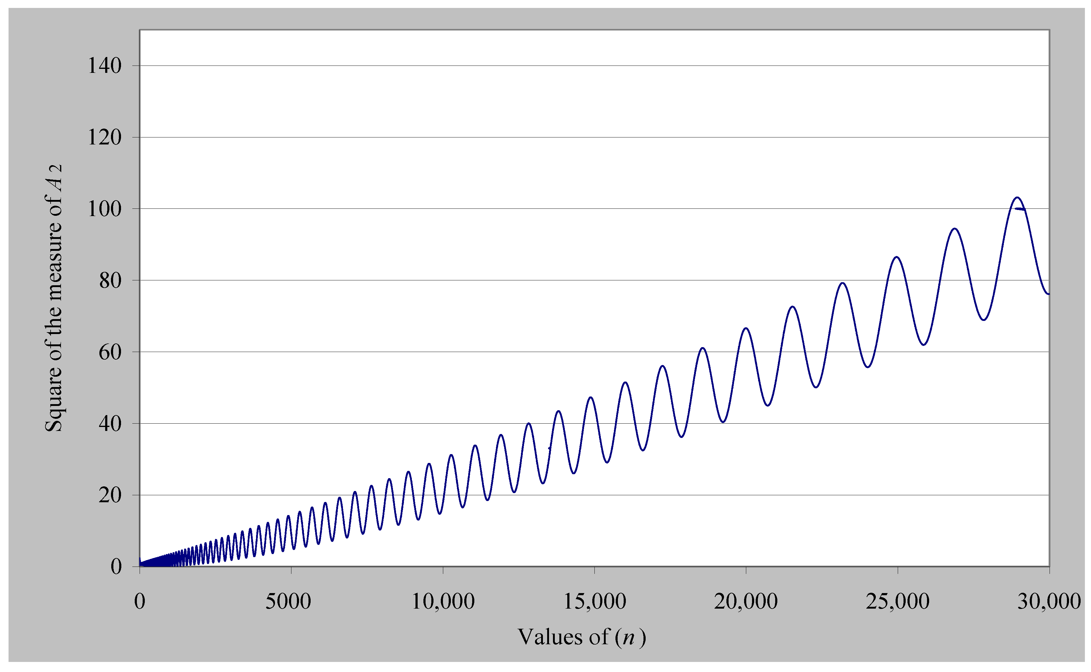
Formula (11), or equivalently Equation (12), gives us the square of the measure of the infinite number A₂(ξ), which for values 0 < α < 1 represents the square of the measure of the zeta function (Dirichlet series described by Equation (1)), which, of course, tends to infinity. Using formula (12), we can numerically calculate |A₂(n)|² with respect to integer values n. 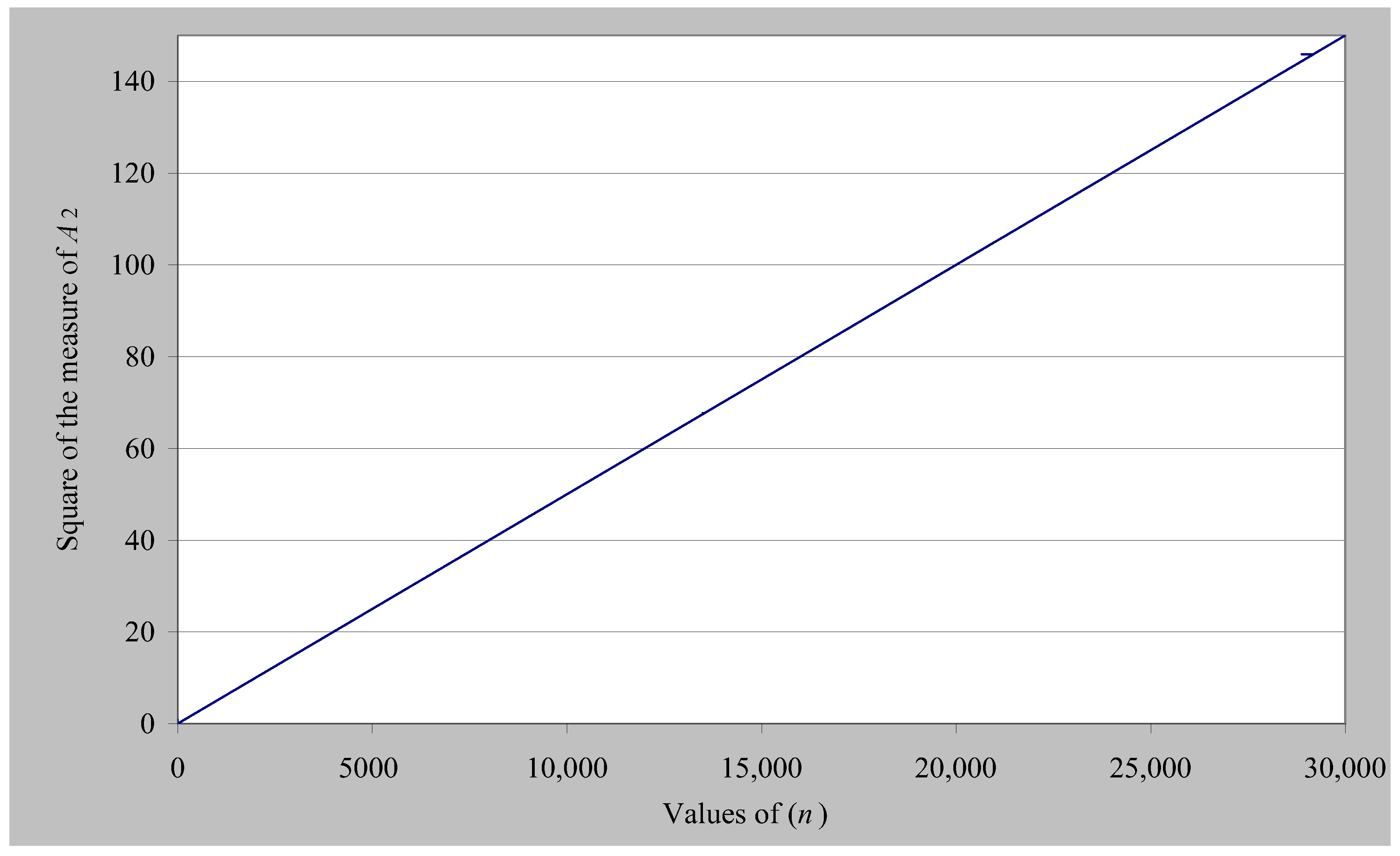Considering α =1/2 and b =16 (i.e., values that do not correspond to a zero of the Riemann zeta function), and obtaining n values up to 30,000, we calculate the diagram shown in Figure 1. In addition, considering α = 0.35 and b = 100 (i.e., values that do not correspond to a zero of the Riemann zeta function, and furthermore are outside the critical line), we also calculate the diagram shown in Figure 2. In both diagrams, we notice that we have a monotonically increasing component and a fluctuating one, as predicted by the theoretical relations (15) and (17). The same conclusion is reached if we take any value that is not a root of the Riemann zeta function.

On the other hand, considering α = 1/2 and b = 14.13472514 (i.e., values that correspond to the first non-trivial zero of the Riemann zeta function), we calculate the diagram shown in Figure 3, where we notice that |A₂(n)|² is monotonically increasing with respect to the integer values of n and, moreover, corresponds to a first-order equation, as can be seen in theoretical Equation (34). In addition, considering α = 1/2 and b = 52.97032148 (i.e., values that correspond to the 10th non-trivial zero of the Riemann zeta function), we calculate the diagram shown in Figure 4, where we notice again that |A₂(n)|² has a first-order equation relation with respect to the integer values of n. We reach the same conclusion if we take any known zero of the Riemann zeta function.

Furthermore, it would be interesting to examine whether relation (30) is confirmed by using a numerical calculation. Firstly, Equation (30) is equivalently written as Equation (44).

$$\underset{n\to +\infty }{\lim }\left(2\left({\displaystyle \frac{1}{\sqrt{1\cdot 2}}}\cos \left(b\ln {\displaystyle \frac{1}{2}}\right)+\mathrm{\dots }+{\displaystyle \frac{1}{\sqrt{1\cdot n}}}\cos \left(b\ln {\displaystyle \frac{1}{n}}\right)+\mathrm{\dots }+{\displaystyle \frac{1}{\sqrt{(n-1)\cdot n}}}\cos \left(b\ln {\displaystyle \frac{(n-1)}{n}}\right)\right)-{\displaystyle \frac{4n}{1+4b^2}}+\ln n\right)+\gamma =0$$

(44)

To this end, let us take a random root of the Riemann zeta function, e.g., the 49th numerically known root, with an accuracy of 11 decimal digits regarding its imaginary part, i.e., the value b =141.12370740402. Also, we obtain n = 40,000, i.e., we obtain the sum of the first 40,000 terms of the corresponding series of relation (44). For this purpose, and considering the large volume of numerical calculations, appropriate code was written in the Visual Basic programming language. Under these conditions, the left-hand side of relation (44) is calculated equal to 0.00000902…, i.e., a value that is very close to zero, thus validating the correctness of relation (44). If instead of n = 40,000, we take a higher value n = 60,000, the left-hand side of the relation (44) is calculated equal to 0.00000013…; therefore, we obtain an even better approximation to zero. Let us now examine the next root of the Riemann zeta function, which is the 50throot, where b =143.11184580762; so, again, for n = 40,000, the left-hand side of relation (44) is calculated to be equal to 0.00000833… (which is also very close to zero), again validating the correctness of relation (44). However, if we obtain a random value between these two consecutive non-trivial roots, for example, b =142.5, then the left-hand side of relation (44) is calculated to be equal to 6.585893…, a value which is not close to zero (like previously); therefore, this valueb =142.1 cannot be a root of Equation (44).

5. A New Numerical Method for Calculating the Zeros of the Riemann Zeta Function Lying on the Critical Line

Equation (30), which is equivalently written as Equation (44), is an analytic equation (of infinite terms) with an unknown variable b; therefore, it can be solved numerically (with the desired accuracy) and give us the values of its roots. It is interesting to note that the roots of Equation (44) with respect to the variable b are also roots of the Riemann zeta function for α = 1/2. However, since relation (19), from which relation (44) was derived, is a necessary and non-sufficient condition (as already explained), it is possible that Equation (44) also becomes zero for other values of the variable b, except for those that are roots of the Riemann zeta function.

For convenience, relation (44) is written equivalently as follows:

$$RES=G-M=0$$

(45)

where

$$G=\underset{n\to +\infty }{\lim }\left(2\left({\displaystyle \frac{1}{\sqrt{1\cdot 2}}}\cos b\ln {\displaystyle \frac{1}{2}}+\mathrm{\dots }+{\displaystyle \frac{1}{\sqrt{1\cdot n}}}\cos b\ln {\displaystyle \frac{1}{n}}+\mathrm{\dots }+{\displaystyle \frac{1}{\sqrt{(n-1)\cdot n}}}\cos b\ln {\displaystyle \frac{(n-1)}{n}}\right)\right)$$

(46)

$$M=\underset{n\to +\infty }{\lim }\left({\displaystyle \frac{4n}{1+4b^2}}-\ln n\right)-\gamma$$

(47)

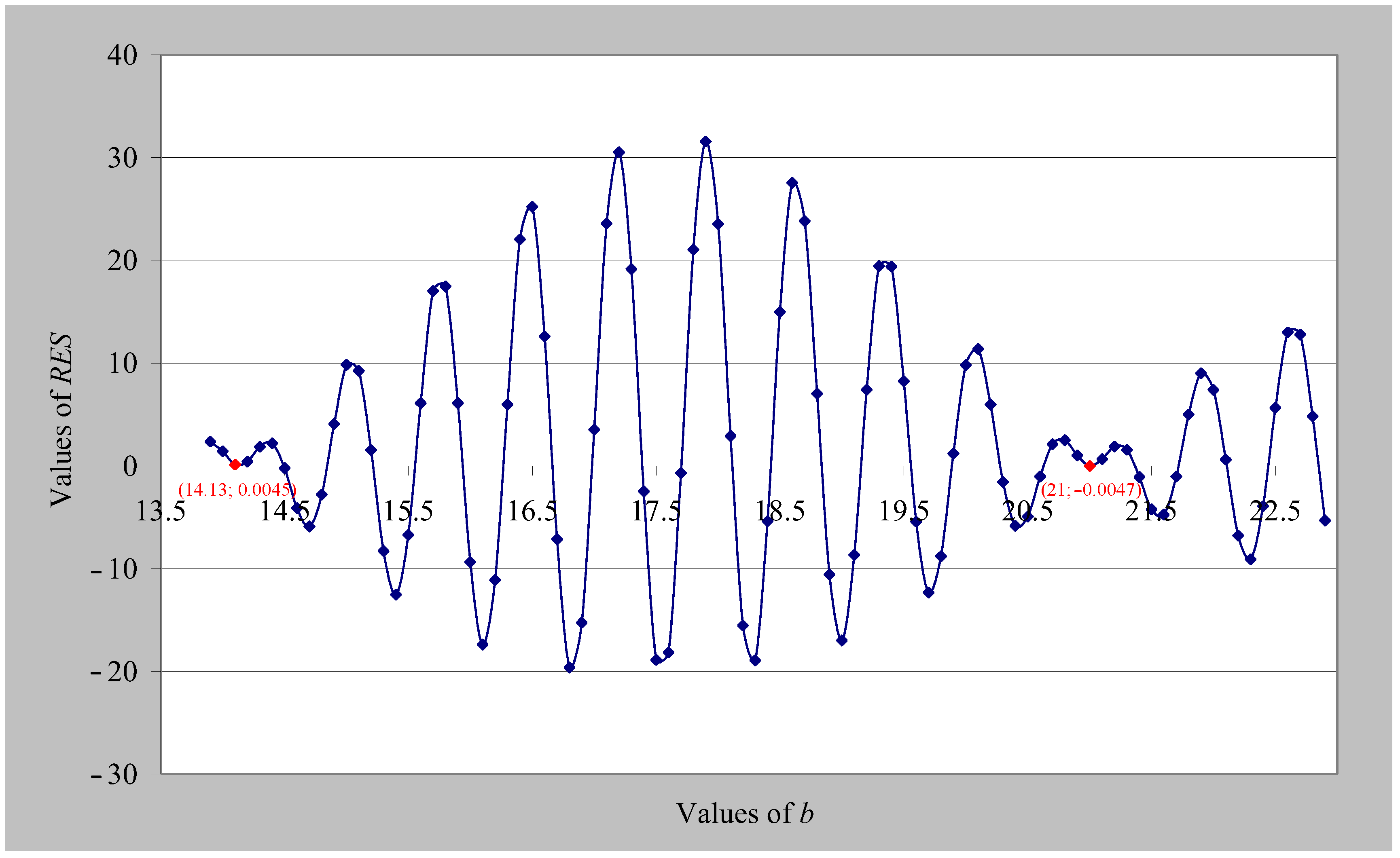
Using the above relations (45)–(47) and assuming a high value of n, e.g., n = 10,000, we can easily numerically calculate, with as much accuracy as we want, the values of the above quantities (M, G, RES).Figure 5 presents the RES values in relation to the corresponding b values, which must certainly be zero at the points where we have roots of the Riemann zeta function. The considered RES values have been calculated for values of b from 13.9 to 22.9, with step intervals equal to 0.1. To this end, appropriate code was also written in the Visual Basic programming language. As can be seen in Figure 5, at point b = 14.13, the value of RES becomes equal to RES = 0.0045, a value which is close to zero. We also notice that for b = 21, the value of RES becomes equal to RES = −0.0047, a value which is also close to zero. As is known, these two values of b correspond approximately to the first two numerically known non-trivial roots of the Riemann zeta function.

If we want a higher precision of the b value, e.g., for the first non-trivial root of the Riemann zeta function, we can iteratively use the same relations (45)–(47), gradually increasing or decreasing the b value and checking each time the corresponding value of RES, so that it continuously decreases (in absolute values) and tends toward zero. In this way, for b = 14.134, we obtain RES = 0.002476; furthermore, for b = 14.134725, we achieve an even higher accuracy (a better approximation to zero), namely RES = 0.002452. Therefore, the value b = 14.134725 is a good approximation (accuracy of six decimal digits) of the imaginary part b of the first non-trivial root of the Riemann zeta function. Consequently, the first non-trivial root of the Riemann zeta function is equal to 1/2 + i14.134725…, a value that coincides with the known value from the literature. 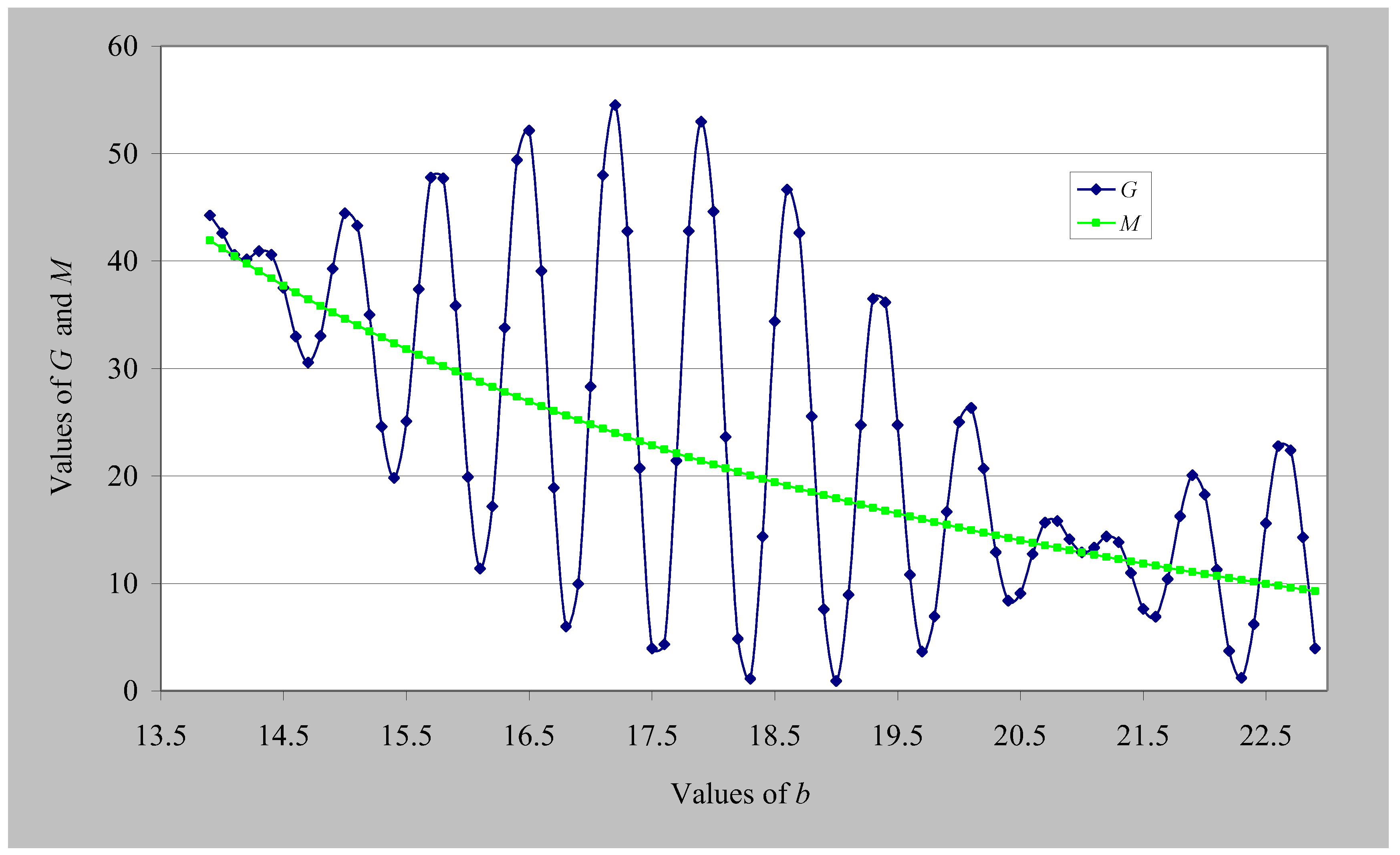Figure 6 presents the values of G and M for b values from 13.9 to 22.9, respectively, with a change step of b as before, i.e., equal to 0.1.

However, as we can see in Figure 5, between the aforementioned twob values, which correspond to the first two non-trivial roots of the Riemann zeta function, there are additional 18 points where the function RES(b) also becomes zero (it intersects the horizontal axis in the diagram shown in Figure 5). However, as already mentioned, relationship (44) and, consequently, relationships (45), (46), and (47), which are derived from (44), constitute a necessary but insufficient condition. In other words, there may be other values of b in addition to those corresponding to a root of the Riemann zeta function, which also makes Equation (44) zero, as well as Equation (45). How, then, will the distinction be made?

As we have seen before (Equation (36)), a condition for having a root of the Riemann zeta function when α = 1/2 is the non-fluctuating G(n) quantity (absence of sinusoidal functions). Therefore, considering Equation (45), in order to have a root of the Riemann zeta function, the RES quantity also ceases to fluctuate. Therefore, this criterion distinguishes between the b values that correspond to roots of the Riemann zeta function and the rest that do not. This conclusion can be confirmed numerically by taking a different value of n, e.g., n = 5000 instead of n = 10,000, where we observe that RES intersects the horizontal axis at different values, except for the points that have roots. Figure 7 presents both RES(b) diagrams, for n = 5000 and n = 10,000. Indeed, we observe that apart from the two known roots (b values) of the Riemann zeta function, where the corresponding RES values converge to zero (for both n = 5000 and n = 10,000 as shown in the zeroing points enclosed by green circles), for the remaining b values, the corresponding RES values do not converge but fluctuate sinusoidally.

We can now see, for α = 1/2, how many and which roots of the Riemann zeta function exist in the interval of values of b from 105 to 110. In Figure 8, we can see the values of RES for b ranging from 105 to 110, with a step change in b equal to 0.1, where n = 10,000. We notice that close to the value b = 105.5, as well as close to the value b = 107.2, there are the roots of the Riemann zeta function known from the literature, which we can calculate with as much precision as we want based on Equations (45)–(47). We also notice that there are five other points where the RES(b) function becomes zero (crosses the horizontal axis); however, at these points, the non-fluctuating condition is not satisfied. Therefore, using this numerical method, we can calculate on the critical line (α = 1/2), in any interval of values of b, how many and which exact roots of the Riemann zeta function exist.

This numerical method is simple and effective and gives results in a short time, of course depending on the desired accuracy of the results, that is, the number of decimal digits of the solution. For an accuracy of two to three decimal digits, the method gives results in a few minutes. The reason is that Equations (45)–(47) to be solved are simple. The relevant code in the Visual Basic programming language consists of less than 50 commands. Of course, the method offers the possibility to calculate the solution with as many decimal digits as we want, increasing the calculation time accordingly.

6. Conclusions

This study attempted an in-depth investigation of the Riemann zeta function and revealed important aspects of it from a different point of view. The study introduced a new mathematical framework to analyze the non-trivial zeros of the Riemann zeta function, using infinite numbers and rotational infinite numbers. The application of infinite numbers as a tool to study the Riemann zeta function is innovative and provides a fresh perspective on an extensively researched problem. Using these numbers and their properties, an interesting correlation between the non-trivial zeros of the Riemann zeta function lying on the critical line was revealed and demonstrated. Moreover, a relation between the Euler–Mascheroni constant (γ) and the non-trivial zeros of the Riemann zeta function (which also lie on the critical line) was discovered and proved. In this way, constant (γ) can be defined in a different way, as a limit of a series that includes any one of the infinite non-trivial zeros of the Riemann zeta function. Furthermore, based on this analysis, complex limits of series and ratios of series were presented and proven. In addition, it was shown that for complex values, s = α + ib (0 < α <1), which do not correspond to the zeros of the Riemann zeta function, the corresponding Dirichlet series, which certainly tends to infinity, includes a monotonically increasing component and a fluctuating one. However, when the α and b values correspond to zeros of the Riemann zeta function lying on the critical line, the fluctuating component of the corresponding Dirichlet series vanishes and the Dirichlet series grows linearly toward infinity. The previous theoretical results were fully confirmed numerically and clearly explained with illustrative corresponding diagrams. Finally, a new numerical method was presented with explanatory diagrams for the identification and numerical calculation of the roots of the Riemann zeta function that lie on the critical line. More specifically, the method can calculate how many and exactly which roots of the Riemann zeta function exist within a range of b values on the critical line (α = 1/2). In conclusion, the use of ordinary/rotational infinite numbers has illuminated different aspects of the Riemann zeta function, hitherto unknown, and made it possible to analyze and solve mathematical relations that are otherwise very difficult or impossible to solve using conventional methods. Such relations are like those appearing in Equations (10), (29), (30), (38), and (43), which are not easy to prove without the use of infinite numbers. Finally, in a future article, the Riemann Hypothesis will be investigated using the infinite numbers and the new possibilities they offer.