1. Introduction
Carbon dioxide (
) emissions worldwide continue to rise, and as a result, environmental sustainability is at risk; using correct and accurate models to predict emission rates of
is central to reducing the impact of climate change. Sophisticated forecasting models are essential not only for the development of specific strategies but also for the tracking of emission dynamics on a macro level [
1,
2]. The traditional way of developing prediction models is insufficient for such a case in general because of the nature of environmental data, which carries non-linear and random characteristics and is time-variable. These limitations have led to a search for better methods, especially those reinforced with artificial intelligence (AI) techniques based on fundamental concepts of machine learning (ML), which have been improved with optimization techniques [
3].
Machine learning models have recently been used widely in environmental data analysis because of their ability to find patterns and correlations in the datasets. However, the performance of these models has a strong link to the algorithms used in them, mainly when it comes to time-variant sequences like
emission [
4,
5,
6]. This research’s first approaches apply a set of preliminary yet sufficient ML models, namely Cat Boost, Gradient Boosting, Extra Trees, and XGBoost, which are well known for their stability and versatility in working with structured data. These ensemble learning methods, developed based on gradient-based optimization, offer an excellent baseline for the predictions made. However, they cannot model long-term dependencies effectively as they are inadequate in considering essential sequential details of the time series dataset [
7,
8,
9].
To address these limitations, this study advances to sophisticated Recurrent Neural Network (RNN) architectures, particularly Gated Recurrent Unit (GRU) variants. Three advanced architectures are emphasized: Bidirectional GRU (BIGRU), Stacked GRU, and Attention-enhanced BIGRU. BIGRU processes sequences bidirectionally, enhancing temporal relation capture [
10], while stacked layers enable hierarchical feature learning. Attention mechanisms further improve focus on critical time steps [
11,
12,
13].
The study introduces two novel optimization algorithms: Greylag Goose Optimization (GGO) and Al-Biruni Earth Radius (BER). GGO mimics avian collective behavior to balance exploration–exploitation [
14,
15,
16], while BER employs geometric principles for convergence in noisy optimization spaces [
17,
18,
19]. Their hybridization in GGBERO enables robust feature selection and model tuning.
The effectiveness of the proposed models and the optimization strategies is assessed using statistical techniques such as the Wilcoxon Signed Rank Test and the Analysis of Variance (ANOVA). The Wilcoxon test is useful when rating pairs of samples, allowing the treatment of the interspersed improvements between the models to be significantly improved [
20,
21,
22]. In contrast, ANOVA makes it easier to compare several models based on the given criteria and provide a general evaluation of the difference in performance. Such statistical comparisons are essential to ensure that all the improvements recorded are not because of random chances but the superior methods used in this research [
23,
24,
25].
This study proposes a unified framework for emission prediction using advanced machine learning structures and optimization techniques. The enhanced precision and reliability of the BIGRU model, mainly when the GGBERO algorithm is applied, is a significant finding. The study’s contributions to machine learning and environmental science are substantial, demonstrating the potential of AI-derived models in addressing global issues.
The subsequent sections of this research provide a comprehensive literature review of earlier studies, details of the dataset used, selection of the features, GRU models, and optimization techniques. The model’s success is critically evaluated in the experimental results section, and the key findings are discussed, along with suggestions for further studies.
2. Literature Review
In the literature review, the author focuses on comparing various research works that centered on forecasting carbon emissions with the various models and methodologies applied to enhance the predictive abilities of the forecast models. When governments across the globe press on the need to set ever-higher carbon reduction targets, accurate emission forecasts are inevitable. Of late, with the help of new-age techniques in machine learning and deep learning, efforts have been made to forecast better results. The following section reviews and compares these models across various sectors and regions, and how deep learning may provide better acknowledgment in future emission prediction. Also, the authors present studies that address carbon emissions in transportation, construction, and industrial segments of the economy while stressing the use of model performance indicators such as RMSE, MAPE, and R2. This review focuses on setting out an accurate picture of the role these models can play in achieving improvements in carbon emission mitigation methods.
Authors of [
26] compared the effectiveness of econometric, machine learning, and deep learning models for carbon emission forecasting. Their findings indicate that heuristic neural networks (a deep learning approach) demonstrate higher predictability for future emission forecasting compared to econometric models, though econometric models are more suitable for estimating changes due to specific factors. Also paper [
27] focused on the building and construction sector in China, analyzing emissions across 30 provinces with nine machine learning regression models. Their results show that a stacking ensemble regression model outperformed others, identifying urbanization and population as key drivers of emissions, thus supporting the development of targeted low-carbon policies.
Authors of [
28] addressed embodied carbon emissions in construction by applying artificial neural networks, support vector regression, and extreme gradient boosting to estimate emissions at the design phase. Their models, tested on 70 projects, achieved strong interpretability (R
2 > 0.7) and low error, supporting practical tools for emission estimation and reduction during construction. In addition, authors of [
29] developed an interpretable multi-stage forecasting framework using SHAP to analyze energy consumption and CO
2 emissions in the UK transport sector. Their results indicate that road carbon intensity is the most significant predictor, while population and GDP per capita have less impact than previously thought.
Authors of [
30] utilized XGBoost to analyze real-world driving data for heavy-duty vehicles in the EU, demonstrating that on-board monitoring data enables more accurate CO
2 emission predictions than traditional fuel-based methods. Also paper [
31] introduced an interpretable machine learning approach using land use data to predict emissions in the Yangtze River Delta. Their Extra Tree Regression Optimization model achieved high accuracy (R
2 = 0.99 on training, 0.86 on test data) and revealed spatial clusters of emissions, with industrial land use contributing to regional hotspots.
Authors of [
32] evaluated several machine learning models—including linear regression, ARIMA, and shallow and deep neural networks—for long-term CO
2 emissions forecasting in the building sector across multiple countries. Deep neural networks provided the best long-term prediction performance. Paper [
33] proposed a hybrid deep learning framework combining gated recurrent units (GRUs) and graph convolutional networks (GCNs) to capture both temporal and spatial dependencies in Chinese urban clusters. Their model outperformed baselines in both single- and multi-step forecasts and demonstrated strong generalizability.
Authors of [
34] developed and compared nine machine learning regression models for national-level CO
2 emissions, finding that optimized Gaussian Process Regression achieved the highest accuracy (R
2 = 0.9998). Paper [
35] used ARIMA, SARIMAX, Holt-Winters, and LSTM models to predict India’s CO
2 emissions, with LSTM achieving the lowest MAPE (3.101%) and RMSE (60.635), confirming its suitability for emission forecasting.
Paper [
36] applied deep learning, support vector machines, and artificial neural networks to forecast transportation-related CO
2 emissions and energy demand in Turkey, finding strong correlations between economic indicators and emissions, and predicting significant increases in both metrics over the next 40 years. Also Authors of [
37] used reinforcement learning to optimize ship routes, reducing fuel consumption and emissions. The DDPG algorithm achieved the best performance, demonstrating the potential of RL for emission reduction in shipping.
Authors of [
38] forecasted greenhouse gas emissions in Turkey’s electricity sector using deep learning and ANN, achieving high accuracy across several metrics, and highlighting the rapid growth of GHG emissions in recent decades. Also paper [
39] used LSTM models for high-frequency greenhouse gas emission prediction in transport networks, outperforming clustering and ARIMA models and supporting the use of deep learning for detailed, real-time emission forecasting. In addition paper [
40] improved CO
2 emission prediction in China by combining factor analysis with a PSO-optimized extreme learning machine (PSO-ELM), achieving higher accuracy than conventional ELM and backpropagation neural networks. Their approach supports more effective economic policy design for emission reduction.
Table 1 shows a comparative analysis of various studies on forecasting carbon emissions using different models and methodologies. The table captures key aspects, including the type of model used (deep learning, machine learning, econometric models), the main sector or region studied, performance metrics, and key findings. The comparison highlights that deep learning and machine learning models often exhibit higher accuracy and better prediction capabilities, particularly when applied to spatial–temporal data or in complex systems like transportation and construction. Moreover, econometric models tend to excel at estimating changes due to specific factors but may lack the predictive power of more advanced models. These findings align with the general trend in the literature, where machine learning models, especially ensemble and deep learning approaches, are increasingly favored for their adaptability and improved performance across diverse datasets and sectors.
As illustrated in this literature review section, various mitigation techniques and technologies are highlighted above to show how diverse they are for reducing from vehicles. The studies we analyzed above describe various strategies to reduce car emissions, such as regulation, technological, and other policy options. Though there has been some success in making transportation systems cleaner and more efficient, issues still need to be addressed, including the lack of infrastructure and customer acceptance to implement policies. A multidimensional strategy incorporating technological innovation, supportive policies, and social participation will have to be employed in the future to achieve significant reductions of emissions from vehicles collectively. The insights gathered from these studies thus create room for a greener and more effective transit environment. Policymakers can use the studies, business stakeholders, and researchers to assist them in decision-making as the world strives toward sustainability, promoting climate resilience.
Following the literature review, the key research gaps identified in this study are summarized as follows:
Inadequate handling of non-linear, time-dependent patterns in CO2 emissions data by traditional models;
Limited capacity of existing methods to capture long-term sequential relationships;
Insufficient integration of advanced optimization techniques for feature selection and hyperparameter tuning;
Absence of a unified framework combining deep learning architectures with hybrid optimization strategies.
To address these identified research gaps, this paper proposes the following methodological contributions:
Development of a unified framework integrating advanced GRU architectures with hybrid GGBERO optimization;
Demonstration of GGBERO-optimized BIGRU’s superior performance (MSE: 1.0 × 10⁻⁵);
Novel hybrid optimization strategy enhancing model robustness against local optima;
Comprehensive validation using the Wilcoxon Signed Rank Test and ANOVA;
Interpretable insights into emission drivers through attention mechanisms.
Collectively, these contributions fill the research gaps identified and enhance the existing carbon emission prediction by presenting a reliable, interpretable, and statistically proven modeling framework. It makes a sound foundation for future studies and applications in environmental data analysis and policymaking.
3. Materials and Methods
This section describes the research methods used in the study and the data used to develop the models from the data collection. Therefore, this research aims to achieve a high level of accuracy and reliability in predictions for emission levels and identify the hidden links between vehicle attributes and emissions through data analysis and feature selection methods coupled with state-of-the-art optimization techniques.
3.1. Dataset
The dataset adopted in this research provides clear insights into how different aspects of a vehicle affect the emission of
, hence creating a platform to model and accurately predict the same emissions. The dataset originates in the Canadian government’s official open-data portal and is seven years long, where variables are represented in 7385 rows and 12 columns, respectively. Every row is associated with a specific vehicle entry and contains crucial variables, which either interactively or non-interactively convey their impact on the vehicle’s
emissions. Since the data are collected over several years, identifying trends and patterns that may be typical of old and newer models will be more precise [
41].
The characteristics of the dataset cover aspects of basic vehicle description, including model type, transmission system, refueling type, and fuel consumption rates, all of which are crucial to defining a vehicle’s emission factors. All these features are named using standard four-letter alphanumeric codes for ease of analysis. For instance, the vehicle model is categorized based on its drivetrain configuration and body structure, including options such as four-wheel drive (4WD/4 × 4), all-wheel drive (AWD), flexible-fuel vehicles (FFV), as well as short (SWB), long (LWB), and extended wheelbases (EWB). These distinctions are critical, as they directly relate to the vehicle’s performance and, consequently, its emissions.
Transmission types are similarly encoded, covering a range of systems from fully automatic (A) to automated manual (AM), continuously variable (AV), and manual transmissions (M). Additionally, the dataset records the number of gears, reflecting the variability in gear configurations that can influence fuel efficiency and emissions. The inclusion of this level of detail allows for a more nuanced analysis of how transmission technology impacts output, acknowledging the complex interplay between gear ratios and driving conditions.
Fuel type is another critical variable, with categories including regular gasoline (X), premium gasoline (Z), diesel (D), ethanol (E85), and natural gas (N). Each fuel type has distinct properties affecting combustion efficiency and emission levels. For instance, diesel engines, while typically more fuel-efficient than gasoline, emit higher levels of certain pollutants, making this a key consideration in emission modeling. On the other hand, ethanol-blended fuels present a different profile due to their renewable content, highlighting the diverse factors influencing the dataset.
Fuel consumption is captured in city and highway conditions, expressed in liters per 100 km (L/100 km). A combined rating that blends 55% city driving and 45% highway driving is also provided, along with an alternative measure in miles per gallon (mpg). This dual metric approach offers a comprehensive view of a vehicle’s fuel economy, accommodating metric and imperial systems and enhancing the dataset’s applicability across different contexts. Accurate fuel consumption data is crucial, as it serves as a proxy for understanding how efficiently a vehicle converts fuel into energy and, by extension, its emission levels.
The primary variable of interest in the dataset is emissions, which has the unit of measurement as grams per kilometer (g/km). These figures depict the emissions during the commission of urban and extra-urban driving cycles, which mimic real-world driving typical of usage. The emphasis on output is essential for the present dataset as this indicator is significant in global climate change talks.
The dataset is collected from various government portals, ensuring enough detail and that the level of coverage is needed for model development. The qualities of the data are well-suited to the training and testing of machine learning models to make emission predictions based on vehicle features. Including all these features makes the dataset versatile so that many aspects of the relations between car attributes and their impact on the environment can be investigated.
3.2. Exploratory Data Analysis
Exploratory data analysis, or EDA, is the initial cost-effective step in the data analysis process and forms the basis of understanding the entire dataset and the initial spotting of relations, patterns, or even oddities. EDA is used to analyze the data’s intrinsic structure and identify valuable features that would be used in constructing the subsequent analysis. It makes it possible to establish relationships between variables and to determine the presence of outlying points or potential data distribution patterns, which are crucial for decisions throughout the analysis. To do this, EDA provides an understanding of complex data by displaying it on a heatmap, bar chart, or histogram to combine or prepare such data for a more complicated analysis [
42,
43].
Figure 1 represents a heat map of the correlation of several features of the raw data feed of
emissions and the model before the feature selection occurred, (color: dark orange = strong positive, light = weak, dark blue = strong negative). This means that this heatmap will show the detailed interaction between the variables, where the intensity of the color is a function of the interacting variables. Looking at this heatmap, we can find out if any features are very similar or those that are not contributing much to the model, and thus guide us on which features to keep in the model and which to discard. Sometimes, indicators might be highly correlated; this could be problematic regarding model tuning, particularly within machine learning algorithms.
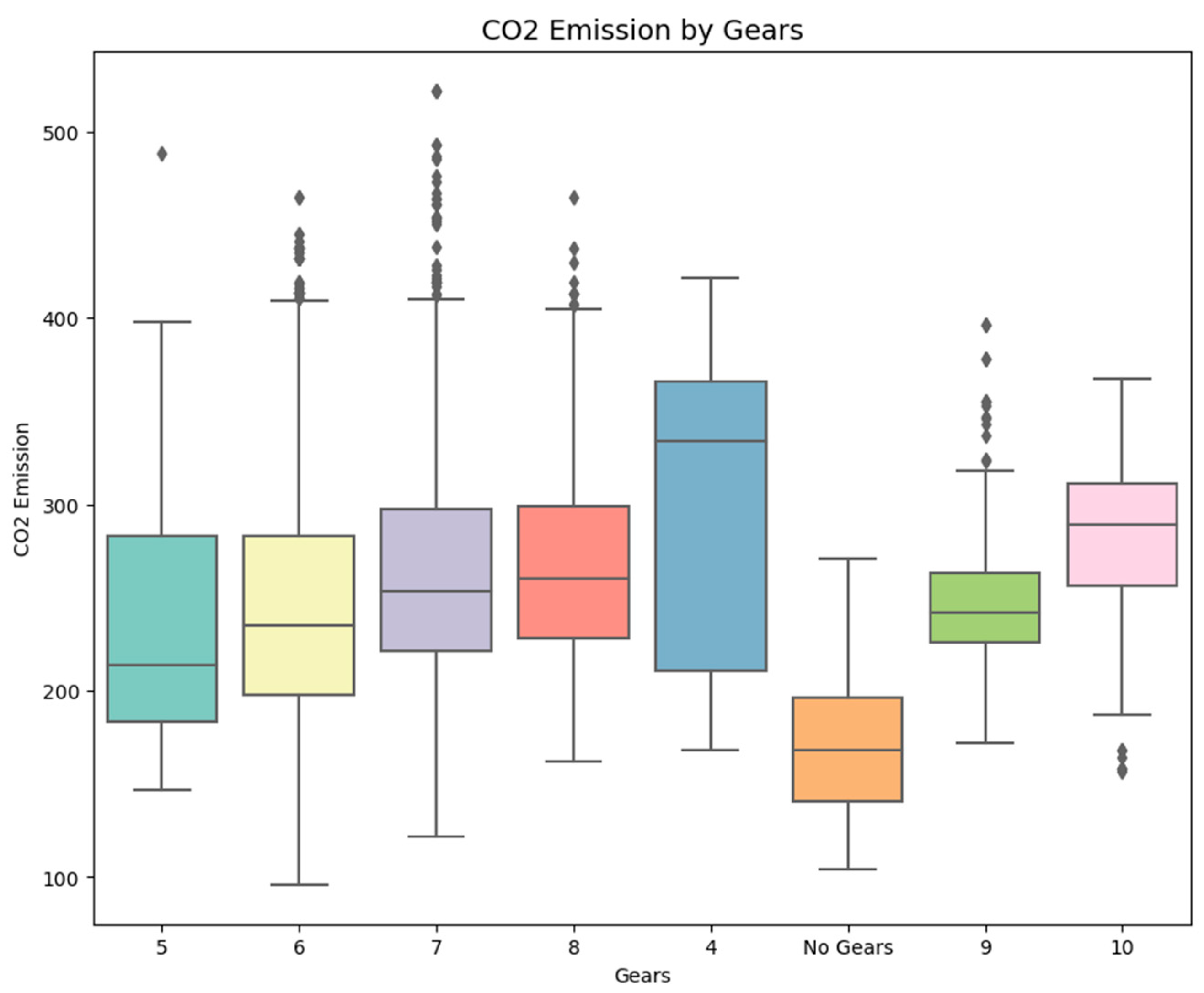
Figure 2 presents the percent share of
emissions of vehicles, depending on the number of gears. It arranges vehicles according to the gear count and then evaluates this aspect’s impact on emissions. The story shows whether cars with more gears have higher or lower emissions, which helps to understand the correlation between gear layout and
production. This analysis is essential to understanding how vehicle mechanics, such as gear systems, influence environmental impact.
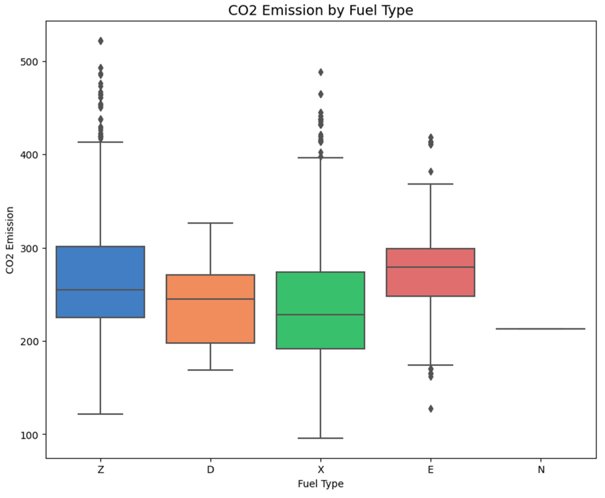
Figure 3 indicates how
emissions vary with each fuel type; how energy forms contribute to emission levels is equally evident. A component-wise plot of gasoline, diesel, ethanol, and natural gas compares them to give a direct perception about which fuel type is emitting high or low emissions. This visualization is beneficial for comparing the environmental impacts of various fuels and can be used to support the push for cleaner energy in automobiles.
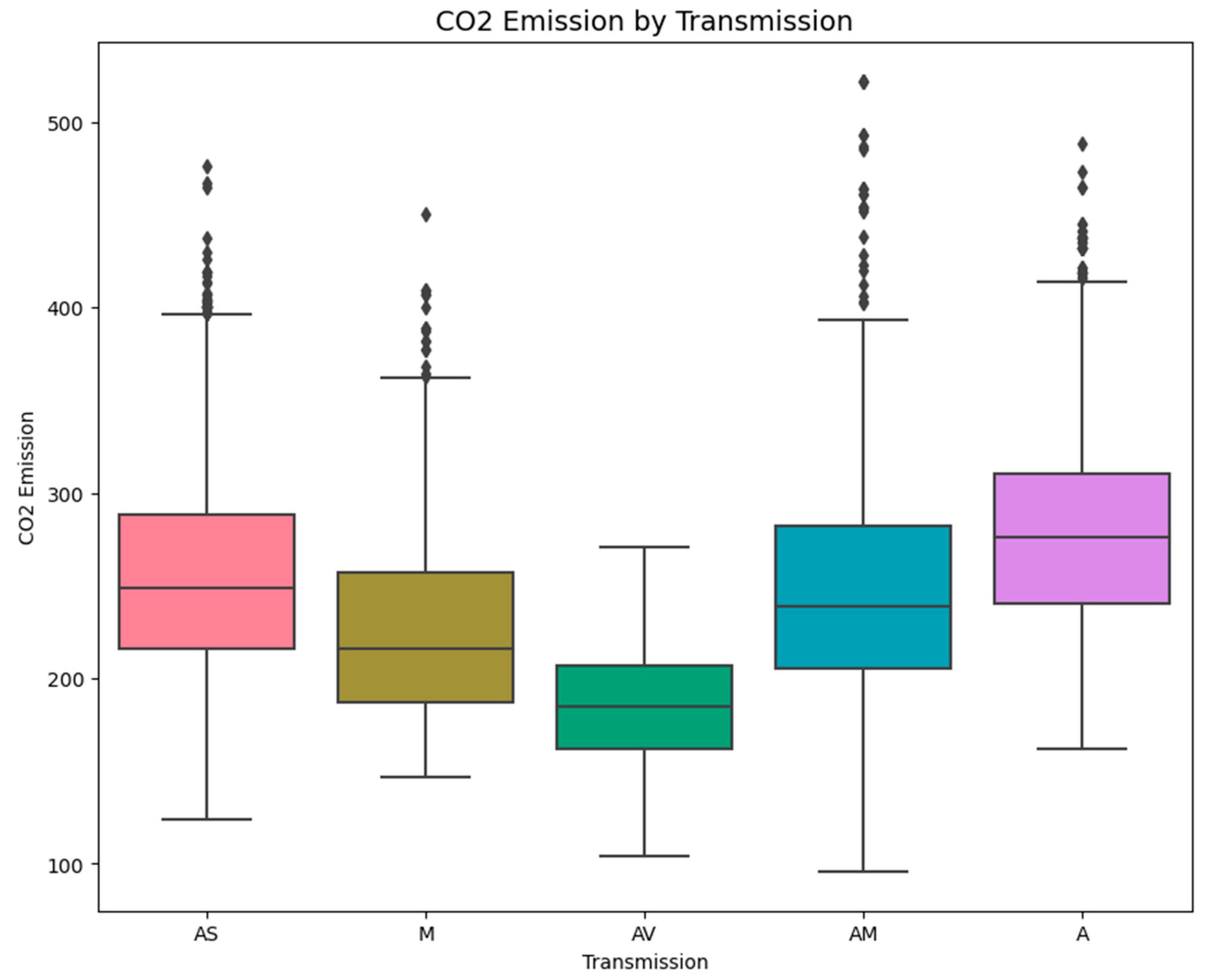
Figure 4 studies the trends in
emissions for the variants in the transmission type: automatic, manual, and continuously variable transmission (CVT). The plot enables the comparison of how transmission technology affects emissions. It is thus essential to determine these differences to evaluate which of the transmission systems is less hostile to the environment and can give some clues to the compromises between power and fuel consumption and emissions.
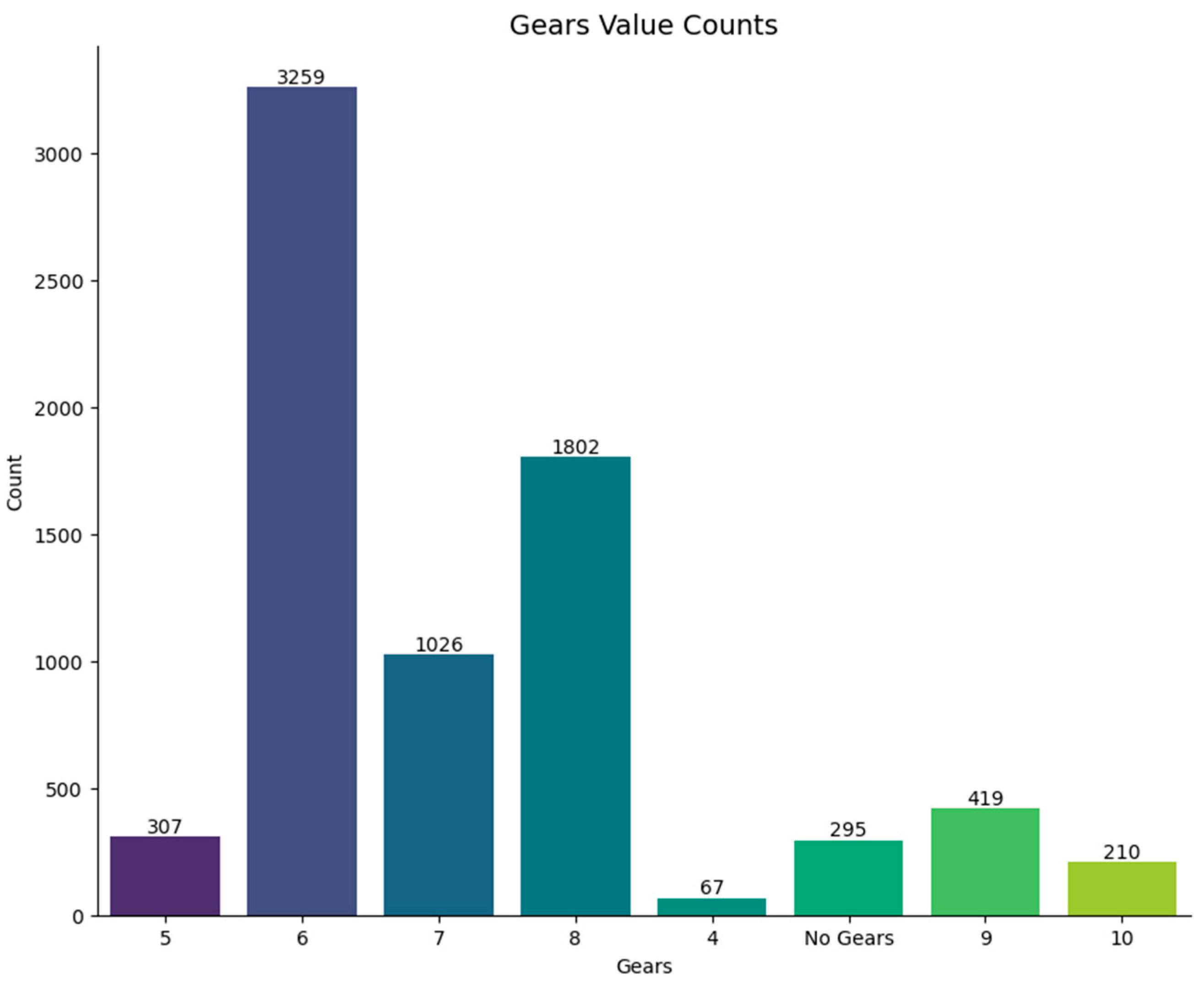
Figure 5 presents the number of vehicles per the number of gears available in each vehicle as a frequency distribution. This bar chart also, in a simple manner, presents information on how frequently each gear configuration is encountered in the dataset. Analyzing gear counts has value because it is a way of defining tendencies in values of vehicle design and fixes for interpreting observed emissions in the analyzed dataset. It also assists in analyzing the utilization of distinct gear configurations and their effect on the environment.
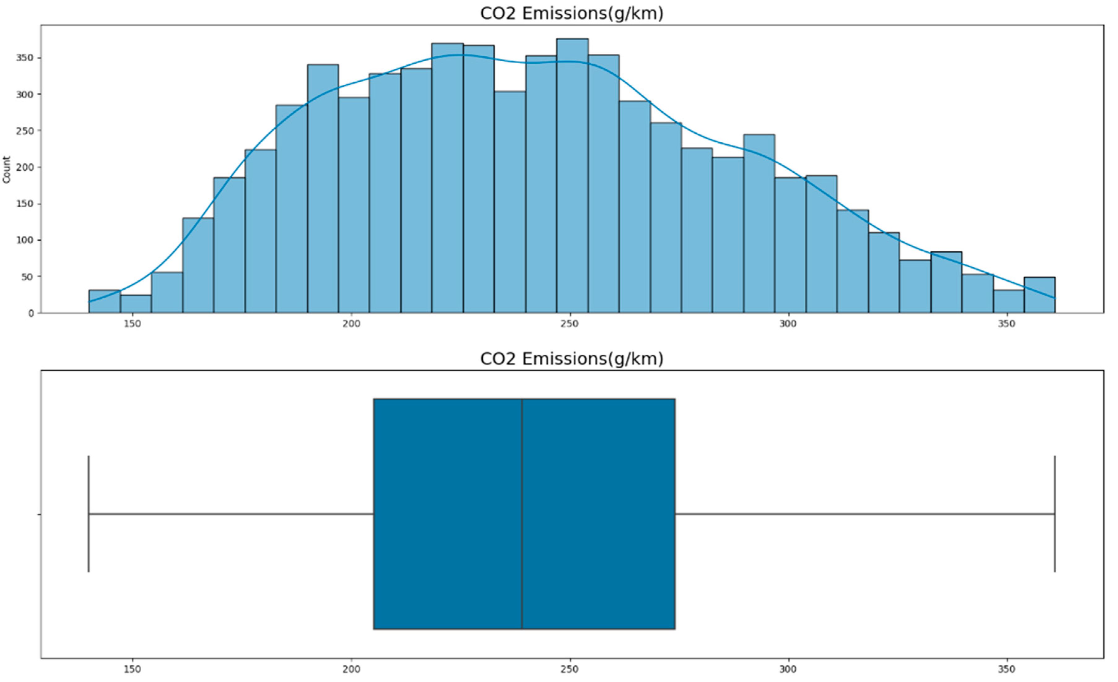
Figure 6 gives a graphical representation of the dispersion of
emissions in all the vehicles in the dataset. The first plot shown is a histogram with a density curve that maps out the distribution of emissions in terms of g/km and how frequent and dispersed they are. The histogram is positively skewed, suggesting that most vehicles produced between 180 and 260 g/km, and few vehicles are in the other bracket. The density curve extends the concept of the histogram more than it enlarges its value, as it smoothens the distribution and looks at the density of data in pollution concentration within any given dataset while amplifying any underlying trends.
The boxplot gives a brief description of the distribution’s most essential characteristics. It provides a median emission value indicated by the line inside the box and the interquartile range (IQR), which is the box’s overall spread. The whiskers go up to the minimum and maximum of 1. Meanwhile, ‘Outliers’ are calculated as 1.5 times the Inter-Quartile Range above the third quartile or below the first quartile. If ‘Outliers’ are calculated in this methodology, this current dataset has no Outliers as it is less than five times the IQR. From this point of view, this boxplot serves the purpose of quickly checking the variability and symmetry of the given dataset and detecting if there is a skewness and/or outliers that might influence further analysis.
Altogether, these visualizations comprise a comprehensive exploratory data analysis that facilitates a deeper comprehension of the factors that shape the values of emissions and subsequent accurate modeling.
3.3. Feature Selection
Feature selection has emerged as an essential step in data analysis since it offers a solution to the problem of high dimensionality by removing features that do not contribute any meaningful information to the analysis. To this end, this optimization seeks to provide the optimal features for the classification and reduction of error in different domains. Feature selection can, therefore, be viewed as a minimization problem optimization [
44]. The solutions are binary values, either zero or one, to enable the identification of features to be included in the optimal model. To convert continuous values to binary ones, the Sigmoid function is utilized:
where
represents the binary solution at iteration
and dimension
, and
is a parameter reflecting the chosen features. The Sigmoid function scales the output solutions to binary values, where the value changes to 1 if Sigmoid (m) is greater than or equal to 0.5; otherwise, it remains at 0.
In the binary optimization algorithm, the quality of a solution is evaluated using the objective equation
, which incorporates a classifier’s error rate (
), a set of chosen features (
), and a set of missing features (
):
where
and
. The k-nearest neighbor (k-NN) classification strategy is commonly used in feature selection to achieve a low classification error rate. While k-NN selects features based on the shortest distance between query and training instances, this experiment does not utilize a k-nearest neighbor model.
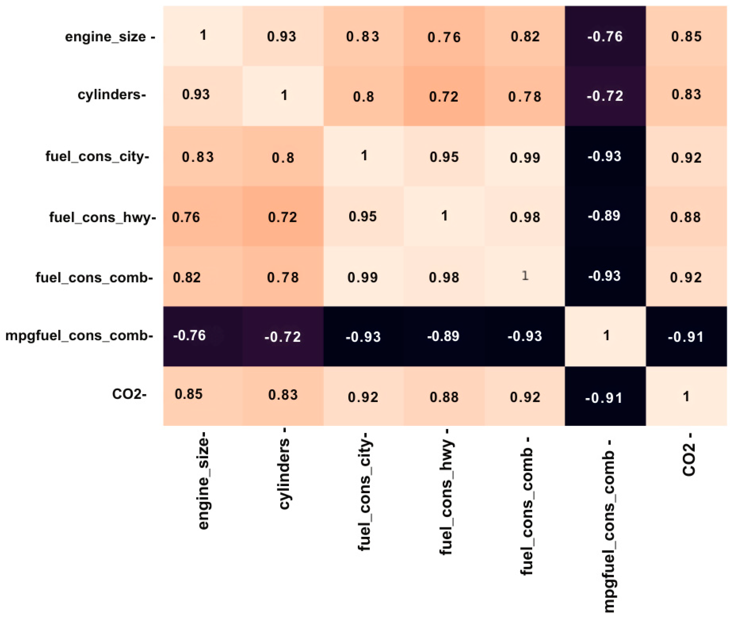
Figure 7 presents a heatmap that visualizes the correlations between critical features in the
emissions dataset after the feature selection process, (color: dark red = strong positive, light = weak, dark blue = strong negative). The heatmap focuses on variables that are most relevant for predicting
emissions, including engine size (L), number of cylinders, fuel consumption (combined L/100 km), and
emissions (g/km). The strength of the correlations is represented by the color intensity, with darker red shades indicating stronger positive correlations and lighter shades indicating weaker relationships.
The heatmap reveals that emissions have a strong positive correlation with fuel consumption (0.92), engine size (0.85), and the number of cylinders (0.83). This indicates that larger engines, more cylinders, and higher fuel consumption are closely associated with increased emissions. The engine size and number of cylinders are also highly correlated (0.93), suggesting that these features are typically aligned in vehicle design.
This heatmap provides valuable insights into the relationships among selected features, helping to confirm that the feature selection process effectively retains the most impactful variables for predicting emissions. The strong correlations highlight vital factors driving emissions, informing the development and optimization of machine learning models.
3.4. Gated Recurrent Unit (GRU) Models
Gated Recurrent Units (GRUs) are one of the most potent types of RNN developed to overcome some of the problems connected with traditional RNNs: vanishing and exploding gradients during training. As for GRUs, they have less architecture in contrast with RNNs since they unify the ‘forget’ and ‘input’ gates into one entity—the ‘update’ gate—which makes them less computationally intensive but, at the same time, capable of capturing dependencies over long sequences. This efficiency makes GRUs especially useful for time series, sequential data, and modeling, where the short- and long-term dependencies are critical to the prediction. In the context of
emission forecasting, long short-term memory deep bidirectional RNNs known as GRU are used to identify temporal dependencies within the datasets and forecast emissions based on the vehicle data retained in the database. Their effectiveness in using gating mechanisms to control the stream of information makes them very effective in this regard [
45].
3.4.1. Bidirectional GRU (BIGRU)
Bidirectional GRU (BIGRU) is a variation of the basic GRU that simultaneously considers past and future context during the training phase. Bidirectional encoding improves the model for analyzing the sequential data because it can notice dependencies between the data that may not be noticeable in a one-directional encoding. This is particularly so in time series prediction tasks such as the study of
emission forecast, where some trends could only be perceived once other future data are available along with previous data. BIGRU can make better predictions by integrating the information from both ends of the sequence because what might be missed by a unidirectional model is complemented by the information from the other end of the sequence. Therefore, BIGRU can capture more relevant information in a given context, such as emission levels that depend on patterns that are not easily identifiable from only a historical or future direction of the time series [
46].
3.4.2. Stacked GRU
However, a single-layer GRU is weak in structure and can only capture simple temporal patterns. This disadvantage is fixed in the Stacked GRU model, which uses multiple layers of GRU to learn hierarchical representations of the input at different levels. In Stacked GRU, the output of each layer is passed on to the next layer, where learn features are improved, and the layers can learn deeper relations in the data. In predicting
emissions, the Stacked GRU architecture allows the model to have a complex interdependence between various time scales, ranging from short to long. Such layering provides the model with granularity and makes the high-frequency identification more accurate and grounded on the low-frequency understanding of a process. The same component also makes the model learn better from the hierarchical form of the input sequences and thus generalize well to the unseen data [
47].
3.4.3. Attention-Based BIGRU
The Attention-based BIGRU model integrates attention mechanisms and BIGRU to improve focus on the significant parts of the input sequence for the prediction. Contrary to what happens in static models, in time-series forecasting, not all time steps contribute the same output. The features help to give different importance to the steps, allowing the model to focus on the moments that are more important for the final decision. When paired with BIGRU, the attention mechanism can enhance the mechanism of employing past and future contexts, with the capacity to weigh the most critical inputs in its present. In particular, the combination of the two features proves helpful for
emission prediction: the points marked as significant by the model can be either specific fuel consumption changes or variations in some driving conditions, which could be more relevant for
emissions. The attention mechanism allows for the dynamic selection of focused and unfocused parts of the input, which increases the interpretability and accuracy of the model, so it is suitable for sequential prediction problems [
48].
3.5. Optimization Algorithms
3.5.1. Greylag Goose Optimization (GGO) Algorithm
The GGO algorithm has been derived from the Greylag goose, including successful phases like the Embarking, Take-off, and Landing phases, as well as social behaviors like V-formations, Wiggling, and Muscular trembling. As mentioned, geese form a very tight-knit society and work together on most of the tasks used in the GGO algorithm. Geese are monogamous, partners for life, and may even create a protective circle around their offspring. Such a coherent social organization can be seen in the GGO view of the optimization process, where all people within the population contribute to the solution.
In the wild, there is a more prominent organization that they form known as gaggles; the members act and protect one another, and they even take turns to employ themselves. This is mimicked by the GGO algorithm, which partitions the population into exploration and exploitation populations at different stages. All these groups must search the solution space—the roles are shared by having everyone shift from exploring (finding new solutions) to exploiting (fine-tuning solutions found already). They do this similarly to the geese, achieving harmonized, efficient flight by flying in a ‘V’ formation so that the lead goose helps create less resistance for the rest of the formation.
The GGO algorithm starts by creating a population of potential solutions. It is like the population division in genetic algorithms, where individuals can be an exploration or exploitation type, modified based on performance. Exploration is looking for new regions within the solution space. In contrast, the leader (the best solution) guides the exploration group, whereas exploitation works to enhance solutions in the leader’s proximity. The mentioned division enables the algorithm to prevent premature exploitation while providing a reasonable level of exploitation.
Exploratory activities of GGO make a comprehensive exploration of the solution space possible. The agents’ positions are changed after using the mathematical formulas that guide promising search areas. After several iterations with no improvement, the algorithm increases the number of agents under exploration, improving the search space for better solutions rather than getting caught up in some local optima. On the other hand, it is the exploitation phase where solutions are refined through the guidance of the agents towards the best solution, which is brought about by the updates of the sentries that have surveillance duties for the quality of solutions.
The GGO flexibility derives from the real-time capability of agents’ shift between exploration and exploitation. The elitist approach used in the algorithm ensures that the best solution is retained and that there is a way of bringing diversity to the population. To accomplish this, the multi-agent architecture of GGO employs a process of continuous role interaction among the agents to interleave the two phases of the search. This is performed iteratively until there is a convergence, and the value with the optimum solution that satisfies the constraints is the output [
49].
3.5.2. Al-Biruni Earth Radius (BER) Optimization Algorithm
The Al-Biruni Earth Radius (BER) algorithm is named in this way because it is based on the idea of the eleventh-century scholar Al-Biruni, who determined the Earth’s radius by measuring the distance between the horizon and the ground from a hill. He initially found out the mountain’s elevation by measuring the angles opposite the peak from two different stations; then, he calculated the amount of Earth’s curvature, that is, the radius of the Earth, by measuring the depression of the horizon from the peak.
Operation with the BER algorithm is based on the increase and decrease of the population split between exploration and exploitation. At the outset, 70 percent of the people are assigned to exploration and 30 percent to exploitation. However, the proportion changes during the optimization stage because the model should pay more attention to refining solutions towards the end. The algorithm also escapes from stagnation by exploring more when no enhancements have been made over several iterations, thus not falling into local optima. Candidate solutions are evaluated iteratively using the fitness function until the best solution is found.
Exploration aims at searching new areas in a defined search space, and exploitation, on the other hand, aims at acceptable tuning solutions. In the exploration strategy, the regions to be explored are chosen, and in the exploitation process, solutions are improved because agents are guided to the best positions. There is also a mutation operation put in use to bring diversification into the algorithm, so the problem of early convergence is not realized. By minimizing and optimizing the size of the population and applying elitism, the BER algorithm guarantees a stable search, along with the best-reported solution across iterations.
It is also important to note that, due to the nature of the algorithm, people switch between exploration and exploitation tasks, which means that the search space does not get approached from the same direction all the time [
50].
3.5.3. GGBERO Algorithm: A Hybrid Approach Combining GGO and BER
The newly proposed GGBERO algorithm combines Greylag Goose Optimization (GGO) and Al-Biruni Earth Radius (BER) to provide the solution set for the global optimization problem. This synergistic approach combines the uncertainty and social interaction in GGO with the exploration and exploitation of BER to improve optimization and accuracy.
The given GGO algorithm emulates how several parties operate to fine-tune how they seek to accomplish their migration aims. Geese working in flight also forward and backward switch their roles so that they can continue working for long distances. In this regard, the GGO algorithm mimics this behavior by dynamically dividing the population by establishing the exploration and exploitation groups. Although many people on the move may end up implementing their ideas while they search for revolutionary solutions, GGO provides constant fine-tuning of the best solutions and enhances the weaknesses within the population based on real-time performance feedback rotation. This flexibility allows the algorithm to escape from the local optima while it progresses towards reaching the global optimum.
In contrast, the BER algorithm leverages an accurate and rather mechanical approach that you shall later learn Al-Biruni employed to determine the Earth’s radius. It emulates the cooperative optimization behaviors observed in swarms, like ant and bee colonies, in which members act in sub-swarms to achieve the same goal. BER also underlines the progress of switching the rates of exploration and exploitation as optimization goes on. This approach moves from a broad exploration of the solutions space to narrow it down, allowing the algorithm to move through the space as an optimization process; it avoids the problem of overspecialization (up to 70%) to maximize the use of the identified solutions. Borrowing from the evolutionary lessons, mutation mechanisms are introduced to guarantee diversity and make the search less susceptible to stagnation, even if the rate of improvement declines.
These strategies complement each other, which is why their combination is possible within the framework of the hybrid GGBERO algorithm, which makes this approach multifunctional. Despite this, in GGBERO, the exploration phase can leverage the dynamics of group-based cooperation that characterizes GGO to search within large solution spaces. At the same time, BER allows fine-tuning processes such as exploration–exploitation, adjusting the number of solution iterations to achieve excellent optimization, and excluding local optima. The advantages and the use of these two approaches make it possible for GGBERO to maintain a high exploration level while incrementally enhancing the quality of solutions, and this delicate balance is crucial when addressing the given kind of task.
Combining the role adaptation, we put into GGO with the subgroup organization and the dynamic rebalancing we proposed in BER, GGBERO improves performance in the exploration and exploitation phases. That is why it is beneficial for solving multimodal problems, for it is critical to keep diversification of solutions and prevent convergence to a local extreme. GGBERO, therefore, is a significant step up from GGO and BER optimization algorithms in that it brings the best of both to bear in optimizing different applications, as shown in Algorithm 1.
| Algorithm 1: GGBERO (Hybrid GGO + BER) Optimization Algorithm |
- 1.
), size . - 2.
Initialize GGO and BER parameters. - 3.
, exploration group size (30%). - 4.
Evaluate fitness for each . - 5.
Identify best solution . - 6.
While do - 7.
% Update exploration phase (GGO-based search) - 8.
for each solution in the exploration group do - 9.
if then - 10.
if (random < 0.5) then - 11.
then - 12.
Update agent’s position: - 13.
else - 14.
Select three random agents: . - 15.
Compute adaptation factor: . - 16.
Update position: . - 17.
end if - 18.
else - 19.
Update position using a sinusoidal motion: . - 20.
end if - 21.
else - 22.
Update individual positions: . - 23.
end if - 24.
end for - 25.
% Update exploitation phase (BER-based refinement) - 26.
for each solution in the exploitation group do - 27.
then - 28.
Compute local adjustments using three sentry solutions: - 29.
. - 30.
. - 31.
. - 32.
Compute updated position: . - 33.
else - 34.
Update position using a refined local search: . - 35.
end if - 36.
end for - 37.
Compute fitness for each . - 38.
Update best solution . - 39.
% Adaptive exploration-exploitation adjustment - 40.
if (Best Fn remains unchanged for two consecutive iterations) then - 41.
Increase exploration group size n1. - 42.
Decrease exploitation group size n2. - 43.
end if - 44.
Set t = t + 1. - 45.
End While - 46.
Return best solution .
|
The performance of metaheuristic algorithms is fundamentally influenced by their parameter settings, as these parameters govern critical aspects of the optimization process such as convergence speed, global search capacity, and avoidance of local optima. In the case of the hybrid GGBERO algorithm—an integration of Greylag Goose Optimization (GGO) and Al-Biruni Earth Radius (BER)—parameter tuning plays a pivotal role in harmonizing the strengths of both component algorithms and ensuring a robust balance between exploration and exploitation.
Parameter Tuning in GGO and BER Within GGBERO
For the GGO component, three core parameters are set: a population size of 30, a maximum iteration count of 500, and 30 independent runs for performance evaluation and statistical robustness. These choices align with the best practices in swarm intelligence, where a moderate population size facilitates diverse solution generation without incurring excessive computational overhead. The iteration count ensures that sufficient cycles of exploration and refinement are allowed, supporting convergence to high-quality optima.
The BER algorithm also uses a population size of 30 and 500 iterations, matching the GGO configuration for consistency in the hybrid framework. Additionally, BER introduces a mutation probability of 0.5, which plays a central role in maintaining diversity and escaping local optima. This probability ensures that half of the solutions are periodically altered, introducing perturbations that increase the search radius when needed. The K parameter, which begins at 2 and gradually decreases to 0 over time, modulates the intensity of the local search, with higher values promoting broader exploration in early stages and lower values enabling fine-tuning during later iterations.
These settings reflect a deliberate temporal adaptation strategy where the algorithm begins with a stronger emphasis on global exploration and gradually transitions toward local exploitation—a strategy often referred to as “exploration–exploitation annealing”. The combination of mutation and decaying K in BER complements the adaptive agent-role switching and flocking behavior in GGO, reinforcing a multi-phase optimization dynamic.
Balancing Exploration and Exploitation in GGBERO
The hybrid structure of GGBERO is explicitly designed to balance exploration and exploitation dynamically, leveraging the respective strengths of GGO and BER. GGO is inherently exploratory, mimicking the collective behavior of geese during migration, where leadership changes and flock formation encourage broad search across the solution space. In contrast, BER excels in local refinement, using historical and geometric cues to intensify exploitation near promising regions.
GGBERO maintains this balance through an adaptive population division. At each iteration, the total population is split between exploratory and exploitative subgroups. If convergence stalls, the algorithm increases the number of individuals allocated to exploration (e.g., by shifting agents from the BER component to GGO-like behavior), thus reinvigorating the search with greater diversity. Conversely, when progress is steady or nearing optimality, the algorithm intensifies exploitation by allocating more agents to BER’s precision-guided search mechanisms.
GGBERO’s feedback loop, based on exploratory objectives such as fitness stagnation and improvement rate, keeps the search away from premature convergence and ensures that the contextually activated global (exploration) and local (exploitation) search has a chance to play a role. This combination of components provides us with the capability to maintain both adaptiveness and resilience across complicated, multi-modal optimization landscapes, especially those in CO2 emission prediction and model tuning.
The core parameter configurations for Greylag Goose Optimization (GGO) and Al-Biruni Earth Radius (BER) algorithms integrated within the GGBERO hybrid optimization framework appear in
Table 2. The algorithms ran through a controlled environment of synchronized population sizes along with a consistent iteration count to maintain stability during the optimization process. GGO uses collective intelligence mechanisms along with dynamic role adaptation, and BER operates through mutation procedures and gradually diminishing control parameters for local search management. The selected parameters created a balanced environment between exploration and exploitation, which led to better performance of the hybrid model during feature selection and hyperparameter tuning.
As a summary, the parameter settings in GGBERO are not only calibrated, but they are also structured in a hybrid manner in the algorithmic side such that the search behavior can be dynamically rebalanced and as a result converges faster, has higher accuracy, and is also robust to both overfitting and getting trapped to local points.
5. Conclusions
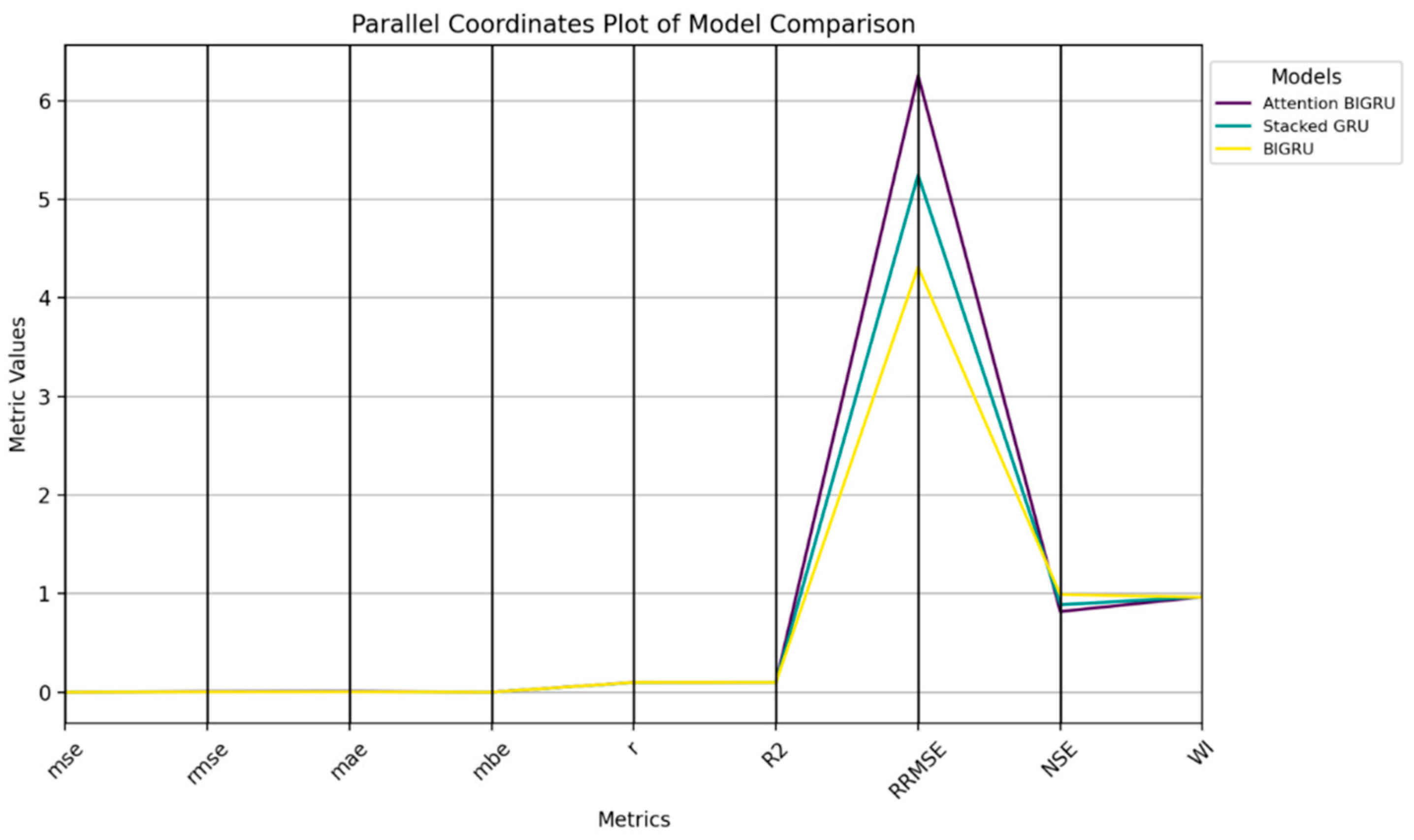
This study offers an extensive review of machine learning models and optimization algorithms for estimating emissions with a concern for feature extraction and model performance. The study presents a new optimization approach referred to as the GGBERO optimization technique, which is a combination of the Greylag Goose Optimization (GGO) and the Al-Biruni Earth Radius (BER) algorithms. The proposed combined GGBERO algorithm, therefore, performed better than its counterparts in terms of selecting the best features that greatly improved predictive measurements, minimized the rate of errors, and improved efficiency in model development. Specifically, ensemble models like Cat Boost and Gradient Boosting were used, where the given basic models delivered higher AUC-ROC than traditional models in terms of identifying non-linear dependencies in the dataset. These models had lower MSE and higher R2 incorporated for high-accuracy tasks, as these models were more suitable. Nevertheless, in comparison with other contemporary recurrent neural network models such as BIGRU, the traditional models of the given family had drawbacks, especially when working with time series that contain long memory dependencies.
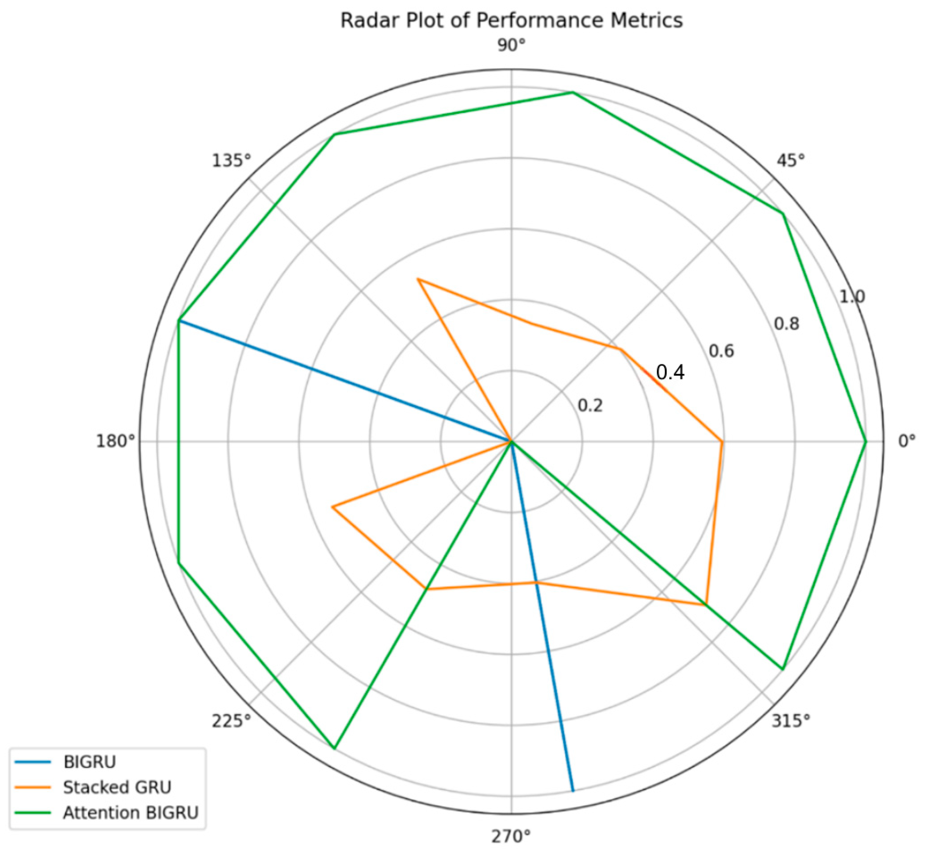
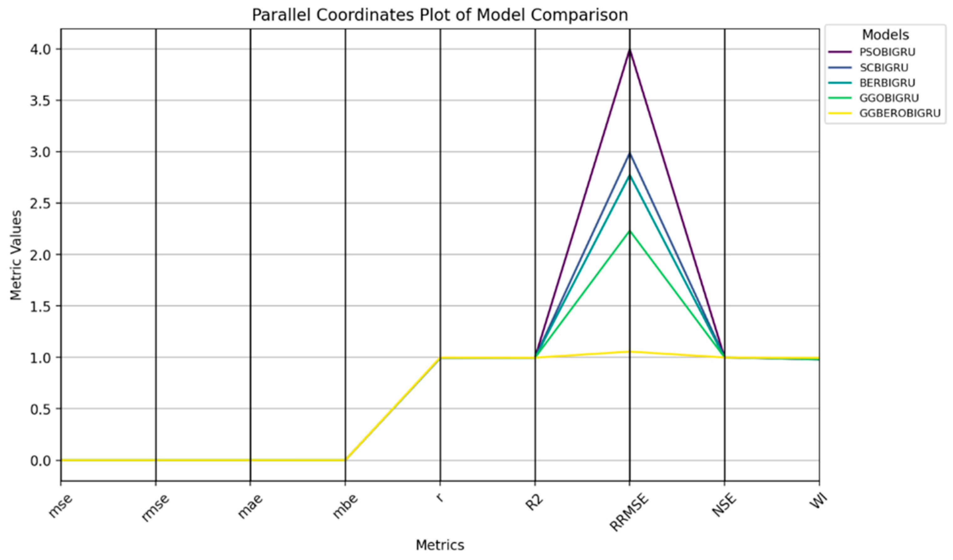
Huge performance enhancements were observed for the BIGRU, the Stacked GRU, and the Attention BIGRU models. Among them, BIGRU owned superior performance due to that it was designed to reveal the forward and backward relation between words and achieved better predictability. The addition of an attention mechanism augments the interpretable and attention-like property of the model and payload attentiveness towards the most relevant temporal positions in the sequence. The BIGRU model used in the proposed GGBERO fashion also provided splendid outcomes, which were far better than the other optimization techniques like GGO-BIGRU, BER-BIGRU, SC-BIGRU, and PSO-BIGRU. The BIGRU optimized for GGBERO was again the model with the lowest errors and the most stable predictions, showing very high R, MSE, RMSE, and R2 values. The discussed hybrid approach was successfully used to balance exploration and exploitation of the solution space, so the model could not get stuck in local optima and had much better convergence characteristics.
The analysis of variance (ANOVA) conducted on the collected results authorized the significant improvements that the driver GGBERO optimization brought. These checks confirmed that improvements in model performance were not accidental, but repeatable, and statistically significant, for different datasets and scenarios.


