A Dynamic Regional-Aggregation-Based Heterogeneous Graph Neural Network for Traffic Prediction

Abstract

Traffic flow prediction, crucial for intelligent transportation systems, has seen advancements with graph neural networks (GNNs), yet existing methods often fail to distinguish between the importance of different intersections. These methods usually model all intersections uniformly, overlooking significant differences in traffic flow characteristics and influence ranges between ordinary and important nodes. To tackle this, this study introduces a dynamic regional-aggregation-based heterogeneous graph neural network (DR-HGNN). This model categorizes intersections into two types—ordinary and important—to apply tailored feature aggregation strategies. Ordinary intersections aggregate features based on local neighborhood information, whereas important intersections utilize deeper neighborhood diffusion and multi-hop dependencies to capture broader traffic influences. The DR-HGNN model also employs a dynamic graph structure to reflect temporal changes in traffic flows, alongside an attention mechanism for adaptive regional feature aggregation, enhancing the identification of critical traffic nodes. Demonstrating its efficacy, the DR-HGNN achieved 19.2% and 15.4% improvements in the RMSE over 50 min predictions in the METR-LA and PEMS-BAY datasets, respectively, offering a more precise prediction method for traffic management.

1. Introduction

With the rapid development of intelligent transportation systems (ITSs) and urban traffic management, traffic flow prediction has become a key task in improving traffic efficiency, reducing congestion, and optimizing road network scheduling. Accurate traffic flow prediction not only provides strong support for traffic planning and real-time scheduling but also effectively alleviates congestion and enhances road safety. As shown in the traffic network diagram in Figure 1, where pentagons represent critical intersections and triangles represent ordinary intersections, accurately predicting different types of intersections can further improve the effectiveness of traffic flow prediction. Therefore, improving the accuracy of traffic flow prediction has become a key issue in current ITS research.

Existing traffic flow prediction methods can be broadly classified into three categories: traditional machine-learning methods, deep-learning methods, and graph neural network methods. Traditional machine-learning methods, such as support vector machines (SVMs), handle nonlinear features through kernel functions but struggle to capture the spatiotemporal dependencies in traffic data. Time-series models, such as long short-term memory (LSTM) networks, can model temporal features but overlook the spatial structure of the road network [1,2]. With the development of deep learning, convolutional neural networks (CNNs) have been introduced to traffic prediction, extracting local spatial features via convolutional kernels. However, their regular grid structure is difficult to adapt to the complex topologies of road networks. In recent years, graph neural network (GNN) methods have emerged, modeling the relationships between nodes through graph structures. However, a significant limitation remains: these methods adopt a unified modeling framework, applying the same treatment to all intersections and regions, which ignores the essential differences in traffic flow characteristics between ordinary and important intersections in the traffic network. To address this issue, it is necessary to perform differentiated modeling of ordinary and important intersections within the traffic network, treating important and ordinary intersections as distinct types of nodes. Based on the importance of different regions, adaptive feature aggregation strategies should be designed.

Moreover, traffic flow data exhibit significant spatiotemporal dependencies, where traffic states are influenced not only by periodic and trend-based factors in the temporal dimension but also by the topological structure of the traffic network and changes in neighboring traffic flows in the spatial dimension. Many existing traffic prediction methods based on graph neural networks typically assume that the traffic network is static, failing to effectively capture the dynamic characteristics of the traffic flow over time. Furthermore, most of these methods rely on homogeneous graph modeling, assuming that the attributes of all the nodes and edges are homogeneous (i.e., the same type and structure). Although this modeling approach simplifies computational complexity in certain scenarios, it often shows limitations when dealing with traffic networks that have complex spatiotemporal dependencies and heterogeneous features. As a result, static homogeneous graph modeling methods cannot comprehensively capture the dynamic, heterogeneous, and regional differences within the traffic network.

In summary, traditional methods face three key challenges: First, existing models generally overlook the heterogeneous features of the traffic network, treating intersections with different functions (such as commercial hub intersections and ordinary intersections) in the same way. Second, static graph modeling methods fail to capture the dynamic characteristics of the traffic flow evolution over time. Finally, there is a lack of effective regional differentiation modeling mechanisms, making it difficult to accurately reflect the impacts of important intersections on the global traffic. These limitations severely constrain the practical value of prediction models.

To address the aforementioned issues, this paper proposes a dynamic regional-aggregation-based heterogeneous graph neural network (DR-HGNN) model for traffic prediction. The main contributions are as follows:

• Heterogeneous graph modeling based on traffic networks: This paper models ordinary and important intersections as different types of nodes through the construction of heterogeneous graphs and processes different regional features through differentiated neighborhood aggregation strategies;
• Dynamic spatiotemporal modeling: This paper introduces a dynamic graph structure to model nodal characteristics in the temporal dimension, dynamically capturing the traffic flow variation patterns at different time points;
• Regional aggregation and a hierarchical attention mechanism: This paper innovatively proposes a dynamic regional aggregation strategy that adaptively adjusts the feature aggregation scope based on the relative importance differences of the target nodes. Additionally, an attention mechanism is introduced to weight the aggregation results from different regions, enabling the model to automatically recognize the relative importance of key regions to the overall traffic flow, further improving the prediction accuracy.

The experimental results show that the DR-HGNN model improves the prediction accuracy by over 15% compared to those of existing traditional methods in the METR-LA traffic flow dataset. By combining dynamic graph modeling and regional aggregation strategies, this paper provides a novel and effective solution for traffic flow prediction.

The structure of this article is as follows: Section 2 reviews the classical methods of traffic flow prediction and the latest progress and limitations of graph neural networks. Section 3 defines the traffic flow prediction task, clarifies the mathematical expressions of heterogeneous graph modeling and dynamic regional aggregation, and provides a framework for the method’s design. Section 4 elaborates on the DR-HGNN model, including the designs of its regional aggregation strategy and attention mechanism. Section 5 verifies the model’s ability to handle complex spatiotemporal dependencies, heterogeneity, and regional differences through experiments and ablation analyses of two public datasets. Section 6 summarizes the main contributions, discusses the application potential of the model in actual traffic management, and proposes future improvement directions.

2. Related Work

2.1. Traditional Traffic Flow Prediction Methods

Early traffic flow prediction methods primarily relied on statistical and physical models. For instance, time-series-based forecasting methods (such as autoregressive models and moving-average models) were commonly used for short-term traffic flow prediction [3,4]. These methods forecast the traffic flow by analyzing trends and seasonal variations in historical traffic data. However, they typically assume that the data are stationary and struggle to handle the nonlinearity and spatiotemporal dependencies inherent in the traffic flow. Additionally, classical regression analysis methods have been widely applied in traffic flow prediction [4,5,6]. Although these methods can provide reasonable predictions in specific scenarios, they fail to effectively capture the complex nonlinear relationships and high-dimensional spatiotemporal dependencies present in traffic flow data.

2.2. Machine-Learning-Based Traffic Flow Prediction Methods

With the rapid development of machine-learning technologies, an increasing number of studies have begun to adopt machine-learning algorithms for traffic flow prediction. Various methods, such as support vector machines [7], random forest [8], and k-nearest neighbors [9], have been widely applied to these tasks. SVMs construct hyperplanes in high-dimensional spaces for classification and regression, enabling them to handle nonlinear problems and, thus, demonstrate good performance in traffic flow prediction. Random forests train multiple decision trees in parallel, providing strong fitting capability and stability when handling high-dimensional data. In addition, neural network methods (such as feedforward neural networks and long short-term memory networks [10]) have been applied to traffic flow prediction. Long short-term memory networks, as a type of neural network that efficiently handles time-series data, are able to capture both long-term and short-term dependencies in traffic flows, especially exhibiting strong performance in short-term flow prediction. Although these methods address nonlinear and temporal dependencies in traffic flows to some extent, they typically fail to fully leverage the spatial structure of the traffic network and the complex dependencies between nodes.

2.3. Graph-Neural-Network-Based Traffic Flow Prediction Methods

Early traffic flow prediction methods based on graph neural networks primarily focused on approaches such as graph convolutional networks and graph recursive networks. Graph convolutional networks (GCNs) [11,12,13] perform convolutional operations on the information of neighboring nodes, effectively capturing the spatial dependencies between the nodes in the graph. Ref. [14] proposed a GCN-based traffic flow prediction method, which applied a GCN to process traffic flow data in road networks, successfully improving the prediction accuracy. Graph recursive networks (GRNs) [15,16,17] combine time-series analysis with graph convolutions, enabling the model to capture temporal dependencies while enhancing its ability to process spatial information. However, these methods often fail to fully account for regional differences in traffic networks, especially the traffic pattern variations at different types of intersections, which lead to limitations in their predictive performances in complex scenarios with significant spatiotemporal dependencies and regional discrepancies. In recent years, dynamic graph neural networks have made significant progress in the field of traffic prediction. Graph WaveNet for deep spatial–temporal graph modeling (Graph WaveNet) [18] improves the model’s adaptability to traffic flow variations by learning dynamic spatial dependencies through an adaptive adjacency matrix. The spatiotemporal hypergraph neural ODE network for traffic forecasting (STGODE) [19] combines spatiotemporal graph neural networks with ordinary differential equations, using continuous-time modeling to better capture the dynamic evolution of the traffic flow. The spatial–temporal dynamic graph convolutional neural network for air quality prediction (T-DGNN) [20] introduces a dynamic graph generation mechanism that can adjust the graph’s structure in real time based on traffic conditions.

As shown in

Table 1. Comparison of the differences between DR-HGNN and other models.

Contrast Dimension	HA	DCRNN	T-GCN	Graph WaveNet	DR-HGNN
Graph structure type	Graphless structure	Static homogeneous graph	Static homogeneous graph	Static homogeneous graph	Dynamic heterogeneous graph
Regional differentiation	no	no	no	no	yes
Spatiotemporal modeling method	Time average	Diffuse convolution + GRU	Spacetime block separation	Adaptive adjacency matrix	Dynamic heterogeneous spacetime convolution
Attention mechanism	no	no	no	yes	yes

, compared to existing methods, the DR-HGNN model proposed in this paper has the following innovations: First, a regional-aggregation-based strategy is introduced, where different aggregation methods for neighborhood nodes of varying orders are applied to different types of regions (such as ordinary and important regions), enabling a better capture of the multiscale characteristics of the traffic flow. Second, by combining the structures of dynamic and heterogeneous graphs, DR-HGNN can dynamically capture traffic flow variations in real time while considering regional differences. These innovations allow the DR-HGNN model to achieve superior performance in handling complex spatiotemporal dependencies, regional heterogeneity, and the heterogeneity of the traffic network.

3. Preliminary Information

Definition 1

(Dynamic Heterogeneous Graph [21]). A dynamic heterogeneous graph refers to a graph structure where the types of nodes and edges not only change across different time steps but also vary within each time step. In a dynamic heterogeneous graph, both the topological structure of the graph and the attributes and types of the nodes and edges evolve dynamically over time. Given a graph $G_t=(V_t,E_t)$, where $V_t$ is the set of nodes at time t, and $E_t$ is the set of edges at time t, each node $v\in V_t$ and edge $e\in E_t$ has distinct types and attributes, and these nodes and edges evolve dynamically as time progresses.

Definition 2

(Lth-Order Neighbors). In a graph, an lth-order neighbor of a node refers to the direct neighbors (i.e., first-order neighbors) of the node as well as the neighbors of these neighbors (i.e., lth-order neighbors). For a node $v_i$, its first-order neighbors are the set of nodes directly connected to $v_i$, denoted as $N_1\left(v_i\right)$, which include all the nodes connected to $v_i$ by edges. The lth-order neighbors are the set of nodes that are connected to the nodes in $N_{l-1}\left(v_i\right)$, denoted as $N_l\left(v_i\right)$, which include all the nodes connected to the first-order neighbors of $v_i$ and are formally expressed as follows:

$$N_l\left(v_i\right)=\bigcup _{v_j\in N_{l-1}\left(v_i\right)}{N}_1\left(v_j\right)$$

In the traffic flow prediction model, the lth-order neighbor aggregation strategy is applied to ordinary regions, focusing mainly on the relationships between the target node and its direct neighbors, as well as the neighbors of those neighbors.

Definition 3

(Region). In a traffic network, a region is a specific geographical area composed of several adjacent traffic nodes and the roads connecting them. The boundaries of a region are typically defined by the multi-order neighbors of different types of nodes.

4. Model

This section provides a detailed introduction to the dynamic regional-aggregation-based heterogeneous graph neural network traffic prediction model (DR-HGNN). Traffic flow prediction relies not only on the static traffic network structure but also on the spatiotemporal dynamics of the traffic flow and the differences between regions. Given the existence of different types of intersections and regions within the traffic network, their impacts on the overall traffic flow vary significantly, especially in traffic-dense areas, such as intersections and commercial districts. Therefore, traditional homogeneous graph methods struggle to fully capture these regional differences, which, in turn, affect the prediction accuracy. To address this issue, this paper proposes a dynamic regional-aggregation-based heterogeneous graph neural network (DR-HGNN).

The model’s structural framework is shown in Figure 2, consisting of four core modules: the ordinary regional aggregation module, the important regional aggregation module, the full regional fusion layer, and the spatiotemporal dependency feature-learning module. The specific tasks of each module are as follows:

Ordinary Regional Aggregation Module: This module primarily handles the ordinary regional nodes in the traffic network. These regions typically refer to areas with relatively stable traffic flows and a small impact on the overall traffic flow, such as T-junctions. For these regions, the fluctuations in the traffic flow are usually small, and their impacts on the global network are limited. Therefore, a simplified neighbor aggregation method can effectively capture their spatiotemporal features. Next, a graph convolutional operation is applied to update the nodal features at time step t, capturing the direct dependency relationships between the target node and its neighbors. Finally, the spatial feature representation of the ordinary regional node at time t is generated to support subsequent predictions.

Important Regional Aggregation Module: This module is designed for important regional nodes, which have significant traffic flow fluctuations and a substantial impact on the overall traffic flow (e.g., intersections near commercial areas). The traffic flow in these areas varies more significantly, requiring more complex aggregation operations to accurately capture their spatiotemporal dependencies. In this module, the traffic nodes near commercial areas are first identified, and their local neighborhood information is propagated along with deeper neighborhood diffusion for feature aggregation. A graph convolutional operation is then used to update the nodal features at time step t. Finally, a richer nodal feature representation at time t is generated, highlighting the key contribution of important regional nodes to the traffic flow prediction.

Full Regional Fusion Layer: First, the aggregated results at time t from both ordinary and important regions are merged to form a unified feature representation. The aggregation information from each region is weighted according to its importance, highlighting the influence of the key regions on the prediction results. By introducing an attention mechanism, the model can automatically learn the weights of features from different regions, thereby determining the contribution of each region to the traffic flow prediction during the global fusion process. The final output is a fused nodal feature representation at time t that combines the features of both ordinary and important regions.

Spatiotemporal Dependency Feature-Learning Module: To further enhance the model’s ability to represent spatiotemporal features, this module aggregates the nodal features from all the time steps using an LSTM network, capturing the dynamic evolutionary patterns of the traffic flow. Through average pooling, this module ensures that the contributions of the nodal features from each time step to the final representation are balanced, eliminating biases between features at different time steps. This allows the model to adapt to the dynamic changes in the traffic network, precisely capturing the spatiotemporal features of nodes at different time intervals. The final result is a comprehensive nodal representation that provides more accurate and dynamic inputs for tasks such as traffic flow prediction.

4.1. Ordinary Regional Aggregation Module

In the ordinary regional aggregation module, the DR-HGNN model aggregates the features of ordinary regional nodes in the traffic network through graph convolutional operations, capturing the spatiotemporal dependencies between nodes. Within the ordinary region, the features of a node are mainly influenced by its direct neighbors (first-order neighbors) and the neighbors of those neighbors (second-order neighbors).

In the ordinary regional aggregation module, the DR-HGNN model updates the nodal features using not only the aggregation of first- and second-order neighbor information but also incorporating dynamic feature increments, $\Delta V\left(t\right)$, which reflect the dynamic changes in the nodal features over time.

For nodes in ordinary regions of the traffic network, the feature update begins with the first-order neighbor aggregation. The feature update of node $v_i$ at time step t is represented as follows:

$$v_i\left(t+1\right)=v_i\left(t\right)+{\Delta }_i\left(t\right)$$

(1)

where $V_i\left(t\right)$ is the feature of node $v_i$ at time t, and ${\Delta }_i\left(t\right)$ represents the feature increment of node $v_i$. The feature increment, ${\Delta }_i\left(t\right)$, is determined by the results of feature propagation through the first- and second-order neighbors as follows:

$${\Delta }_i\left(t\right)=\sum _{v_j\in N_1\left(v_i,t\right)}{W}_1{h}_j\left(t\right)+\sum _{v_k\in N_2\left(v_i,t\right)}{W}_2{h}_k\left(t\right)$$

(2)

where $W_1$ and $W_2$ are learnable weight matrices, and $h_j\left(t\right)$ and $h_k\left(t\right)$ are the features of the first- and second-order neighbors at time t. $N_1(v_i,t)$ and $N_2(v_i,t)$ represent the sets of first- and second-order neighbors of node $v_i$, as defined by the following equations:

$$N_1(v_i,t)=\{v_j\mid (v_i,v_j)\in E\}$$

(3)

$$N_2\left(v_i,t\right)=\bigcup _{v_j\in N_1\left(v_i,t\right)}{N}_1\left(v_j\right)$$

(4)

where $N_1\left(v_i\right)$ is the set of nodes directly connected to $v_i$, and $N_2\left(v_i\right)$ is the set of neighbors of $v_i$’s first-order neighbors.

For the neighbors of the first-order neighbors in the ordinary regional aggregation module, the feature of node $v_i$ is first aggregated by weighted summation with the features of its first-order neighbors, capturing the spatiotemporal dependency between the target node and its direct neighbors. The updated feature increment, ${\Delta }_i^1\left(t\right)$, is computed as follows:

$${\Delta }_i^1\left(t\right)=\sigma (W_2{h}_i\left(t\right)+\sum _{v_j\in N_1(v_i,t)}{W}_2{h}_j\left(t\right))$$

(5)

where $h_i\left(t\right)$ is the feature of node $v_i$ at time t, $h_j\left(t\right)$ is the feature of its first-order neighbor ($v_j$), and $W_2$ is the weight matrix used for learning the weighted features of the first-order neighbors. $\sigma (·)$ represents the activation function (ReLU).

Because traffic flow fluctuations in ordinary regions are generally small and have a lesser impact on the overall network, a simplified aggregation method through the second-order neighbors is sufficient to effectively capture their spatiotemporal features. The feature aggregation using the second-order neighbor feature increment, ${\Delta }_i^2\left(t\right)$, is computed as follows:

$${\Delta }_i^2\left(t\right)=\sigma (W_3{h}_i^1\left(t\right)+\sum _{v_k\in N_2(v_i,t)}{W}_3{h}_k\left(t\right))$$

(6)

where ${\Delta }_i^1\left(t\right)$ is the feature of node $v_i$ after the first-order neighbor aggregation, $h_k\left(t\right)$ is the feature of second-order neighbor $v_k$ at time t, and $W_3$ is the weight matrix used for learning the weighted features of the second-order neighbors.

To prevent feature over-expansion, the model normalizes the aggregated nodal features to ensure consistent scaling after each graph convolutional operation, avoiding the excessive accumulation of information. This normalization is performed using the following formulae, yielding the final nodal feature, $h_i(t+1)$, for ordinary regions:

$${\widehat{\Delta }}_i^l\left(t\right)={\displaystyle \frac{{\Delta }_i^l\left(t\right)}{\sqrt{deg\left(v_i\right)+\gamma }}}$$

(7)

$$h_i\left(t+1\right)=\sigma \left({\displaystyle \frac{V_i\left(t\right)+{\widehat{\Delta }}_i^l\left(t\right)}{\sqrt{deg\left(v_i\right)+\gamma }}}\right)$$

(8)

where $deg\left(v_i\right)$ is the degree of node $v_i$ (i.e., the number of neighbors directly connected to $v_i$), and $\gamma$ is a small smoothing term to avoid division by zero. The index l corresponds to the level of the neighborhood, specifically for the lth-order neighbors of node $v_i$.

4.2. Important Regional Aggregation Module

In the important regional aggregation module, the model primarily focuses on feature aggregation for nodes in the important regions of the traffic network. The aggregation range is extended to capture broader spatiotemporal dependencies. Unlike the ordinary regional aggregation module, important regions (such as intersections near schools and commercial areas) have a greater influence on the traffic flow, so a wider neighbor expansion (up to third-order neighbors) is employed to capture traffic flow information over greater distances.

In this module, the DR-HGNN model aggregates the features of the important regional nodes in the traffic network through graph convolutional operations, capturing the spatiotemporal dependencies between nodes. For nodes in important regions, the feature update is not only based on the aggregation of higher-order neighbor information but also includes dynamic feature increments to reflect the dynamic changes in nodal features.

First, the DR-HGNN model updates nodal features through first-order neighbor aggregation. In the traffic network, node $v_m$ represents an important traffic intersection (e.g., intersections near schools and shops), and its feature update at time step t is given by

$$v_m\left(t+1\right)=v_m\left(t\right)+{\Delta }_m\left(t\right)$$

(9)

where ${\Delta }_m\left(t\right)$ is the feature increment of node $v_m$ from time t to $t+1$, which can be represented by the feature change propagated through first-, second-, and third-order neighbors as follows:

$${\Delta }_m\left(t\right)=\sum _{v_n\in N_1(v_m,t)}{W}_4{h}_x\left(t\right)+\sum _{v_k\in N_2(v_m,t)}{W}_5{h}_y\left(t\right)+\sum _{v_l\in N_3(v_m,t)}{W}_6{h}_l\left(t\right)$$

(10)

where $N_1(v_m,t)$, $N_2(v_m,t)$, and $N_3(v_m,t)$ are the first-, second-, and third-order neighbor sets of node $v_m$ at time t. $W_4$, $W_5$, and $W_6$ are learnable weight matrices; $h_x\left(t\right)$, $h_y\left(t\right)$, and $h_l\left(t\right)$ represent the features of the first-, second-, and third-order neighbors at time t, respectively. The third-order neighbor set, $N_3(v_m,t)$, is computed as follows:

$$N_3\left(v_m,t\right)=\bigcup _{v_k\in N_2\left(v_m,t\right)}{N}_1\left(v_k\right)$$

(11)

By expanding to third-order neighbors, the model captures more distant spatiotemporal dependencies, which are particularly important for traffic hubs or key intersections.

In the important regional aggregation module, because of the larger traffic fluctuations at these nodes, more complex aggregation operations are required to accurately capture the spatiotemporal dependencies. The feature aggregation proceeds by first aggregating information from first-order neighbors, as shown by the following formula:

$${\Delta }_m^1\left(t\right)=\sigma (W_1{h}_m\left(t\right)+\sum _{v_n\in N_1(v_m,t)}{W}_1{h}_x\left(t\right))$$

(12)

where $h_m\left(t\right)$ is the feature of node $v_m$ at time t, and $h_x\left(t\right)$ is the feature of a first-order neighbor, $v_n$, at time t. $W_1$ is the weight matrix used for learning the weighted features of the first-order neighbors, and $\sigma (·)$ represents the ReLU activation function. Then, the feature aggregation is extended to the second-order neighbors as follows:

$${\Delta }_m^2\left(t\right)=\sigma (W_2{h}_m^1\left(t\right)+\sum _{v_k\in N_2(v_m,t)}{W}_2{h}_y\left(t\right))$$

(13)

where $h_m^1\left(t\right)$ is the feature of node $v_m$ after the first-order neighbor aggregation, and $h_y\left(t\right)$ is the feature of a second-order neighbor, $v_k$, at time t. $W_2$ is the weight matrix for learning the weighted features of the second-order neighbors.

Finally, node $v_m$ aggregates information from its third-order neighbors to further capture more distant spatiotemporal dependencies as follows:

$${\Delta }_m^3\left(t\right)=\sigma (W_3{h}_m^2\left(t\right)+\sum _{v_l\in N_3(v_m,t)}{W}_3{h}_l\left(t\right))$$

(14)

where ${\Delta }_m^2\left(t\right)$ is the feature of node $v_m$ after the second-order neighbor aggregation, and $h_l\left(t\right)$ is the feature of a third-order neighbor, $v_l$, at time t. $W_3$ is the weight matrix for learning the weighted features of the third-order neighbors. These operations significantly enhance the model’s ability to capture traffic flow information from more distant nodes, which is crucial for traffic flow prediction in important regions.

As in the ordinary regional aggregation module, feature normalization is applied to prevent the over-expansion of the features. The final nodal feature, $h_m(t+1)$, in the important region is updated based on the aggregation from the first-, second-, and third-order neighbors using the following formulae:

$${\widehat{\Delta }}_m^l\left(t\right)={\displaystyle \frac{{\Delta }_m^l\left(t\right)}{\sqrt{deg\left(v_m\right)+\gamma }}}$$

(15)

$$h_m\left(t+1\right)=\sigma \left({\displaystyle \frac{V_m\left(t\right)+{\widehat{\Delta }}_m^l\left(t\right)}{\sqrt{deg\left(v_m\right)+\gamma }}}\right)$$

(16)

where $deg\left(v_m\right)$ is the degree of node $v_m$ (i.e., the number of neighbors directly connected to $v_m$), and $\gamma$ is a small smoothing term to avoid division by zero. The index l corresponds to the level of the neighborhood (first, second, or third).

This process ensures that nodal features in important regions are accurately updated, enabling the model to effectively capture the spatiotemporal dependencies of the traffic flow, which is particularly important for traffic prediction at key intersections.

4.3. Full Regional Fusion Layer

To effectively integrate these two types of features and ensure that the influence of important regions is emphasized, the full regional fusion layer combines the features obtained from the ordinary regional aggregation module and the important regional aggregation module. It employs an attention mechanism to weight the aggregation results from the different regions.

The full regional fusion layer effectively integrates the features of ordinary and important regions through a regional attention mechanism, with the core innovation being the dynamic weighting of the differential contributions from the two types of regions. Specifically, this layer first receives feature inputs from two parallel modules: the final representation, $h_i(t+1)$, of the ordinary regional node, $v_i$, which captures local traffic patterns through second-order neighborhood aggregation, and the final representation, $h_m(t+1)$, of the important regional node, $v_m$, which captures broader spatial dependencies through third-order neighborhood aggregation.

In the feature interaction stage, the model maps the features from the two regions to a shared semantic space using learnable query–key transformation matrices ($W_q,W_k$), and computes the cross-regional similarity, or attention scores, between ordinary and important regions using scaled dot-product attention as follows:

$${\alpha }_{im}={\displaystyle \frac{W_q{h}_i\left(t+1\right)·W_k{h}_m\left(t+1\right)}{\sqrt{d}}}$$

(17)

where $W_q$ and $W_k$ are the linear transformation matrices for the query and key spaces, respectively; · denotes the dot product operation; and d is the dimension of the nodal features, which is used for scaling to ensure the stability of the dot-product results.

The attention scores are computed using the following formula and then normalized via a softmax operation, resulting in the final attention weight, ${\widehat{\alpha }}_{im}$, which represents the relative importance between the two regions:

$${\widehat{\alpha }}_{im}=\mathrm{softmax}\left({\displaystyle \frac{W_q{h}_i\left(t+1\right)·W_k{h}_m\left(t+1\right)}{\sqrt{d}}}\right)$$

(18)

Using the computed attention weights, the features of both the ordinary and important regions are weighted and summed. The final weighted feature representation of the target node is then obtained. In the feature fusion stage, the weighted aggregation mechanism in Equation (19) constructs a learnable feature-mixing channel. When ${\widehat{\alpha }}_{im}$ approaches 1, it emphasizes the regularity of the ordinary regional nodes, and when it approaches 0, it highlights the influence of the important regional nodes. This adaptive balancing significantly enhances the model’s ability to capture regional heterogeneity.

$$h_v(t+1)={\alpha }_{im}{h}_i(t+1)+(1-{\alpha }_{im})h_m(t+1)$$

(19)

where $h_v(t+1)$ is the nodal feature after the full regional aggregation, and ${\alpha }_{im}$ is the attention weight calculated by the attention mechanism, which reflects the relative importance between the ordinary and important regions. Finally, through this weighted aggregation and attention mechanism, the node’s final feature representation, $h_v(t+1)$, incorporates the spatiotemporal information from both the ordinary and important regions.

The full regional fusion layer brings threefold improvement to the overall model performance: First, by establishing explicit associations between regions, it addresses the issue of feature fragmentation between ordinary and important regions in traditional methods. Second, the dynamic adjustment mechanism of the attention weights enables the model to adapt to the spatiotemporal evolution of the traffic states, such as automatically increasing the weights of important regions during peak hours. Finally, the hierarchical fusion strategy maintains computational efficiency while ensuring that the final feature, $h_v(t+1)$, incorporates both the dynamic characteristics of ordinary regional intersections and the traffic information from important regions, providing a more comprehensive spatiotemporal representation for the prediction module.

4.4. Spatiotemporal Dependency Feature-Learning Module

To further enhance the expressions of spatiotemporal features, the spatiotemporal dependency feature-learning module leverages dynamic graph neural networks (DGNs) and average pooling operations to capture the spatiotemporal dependencies of nodes and generate comprehensive nodal feature representations. These integrated features will serve as inputs for subsequent tasks, such as traffic flow prediction. Specifically, for the nodal features, $h_v(t+1)$, which are obtained from the full regional fusion layer and include the aggregated features from both ordinary and important regions, the spatiotemporal information of each node, v, at time step t is provided.

At each time step, the changes in the traffic flow may lead to variations in the traffic density at certain intersections, which, in turn, can adjust their adjacency relationships. Therefore, the dynamic graph in the model is updated at each time step, depending on the current traffic flow data. For each time step, t, the adjacency matrix in the graph is recalculated to reflect real-time traffic flow changes. The adjacency matrix, $A\left(t\right)$, is updated based on the traffic flow information at each time step. The changes in the adjacency matrix at each time step can be expressed as follows:

$$A\left(t\right)=\mathrm{Update}\left(A\right(t-1),\mathrm{TrafficFlow}(t\left)\right)$$

(20)

where the $\mathrm{TrafficFlow}\left(t\right)$ represents the dynamic changes in the traffic flow, which influence the weights in the adjacency matrix.

To capture the temporal variation in nodal features, long short-term memory (LSTM) networks are used to process the historical feature sequences of each node. LSTM effectively extracts the temporal dependencies of the node and generates a temporal feature representation. First, for each node, v, the module constructs its historical feature sequence, $H_v$, and inputs it to the LSTM as follows:

$$H_v=\{h_v\left(1\right),h_v\left(2\right),\dots ,h_v\left(t\right)\}$$

(21)

This sequence generates the hidden state’s sequence at each time step as follows:

$$S_v=\{s_v\left(1\right),s_v\left(2\right),\dots ,s_v\left(t\right)\}$$

(22)

where $s_v\left(t\right)$ contains the historical information of node v from time step 1 to time step t.

Because the traffic network is continuously changing in real time, the model uses dynamic graph neural networks (DGNs) to dynamically update the graph at each time step according to traffic data, ensuring an accurate reflection of the latest state of the traffic network. As the traffic flow fluctuates, the traffic volumes at intersections may change, which could impact adjacency relationships and edge weights. When performing feature aggregation on the dynamic graph, because different nodes may have varying numbers of neighbors, the model employs an average pooling method to ensure that the contribution of each time step to the nodal features is equal, thus avoiding the over-amplification or neglect of the information.

For each node, v, the average value of its neighboring nodes’ (including its own) LSTM hidden states at each time step is calculated as follows:

$${\overline{s}}_v\left(t\right)={\displaystyle \frac{1}{\left|N\right(v\left)\right|+1}}\sum _{u\in N\left(v\right)\cup \left\{v\right\}}{s}_u\left(t\right)$$

(23)

where $N\left(v\right)$ is the set of neighbors of node v, and ${\overline{s}}_v\left(t\right)$ is the average pooled feature of node v at time step t.

After the LSTM temporal feature extraction and average pooling, the model combines the generated temporal features with the spatial features to form the final integrated nodal feature as follows:

$$h_v^{*}(t+1)=\sigma (s_v\left(t\right)+{\overline{s}}_v\left(t\right))$$

(24)

where $s_v\left(t\right)$ is the hidden state at the final time step of the LSTM, and $\sigma (·)$ is a nonlinear activation function (ReLU). The integrated nodal feature, $h_v^{*}(t+1)$, contains the spatiotemporal feature representation of node v at time step $t+1$, which can be used for subsequent tasks, such as traffic flow prediction and anomaly detection. The dynamic graph neural network module, utilizing LSTM and average pooling operations, captures the spatiotemporal dependencies of nodes and generates more refined nodal feature representations. The LSTM network extracts the historical features of nodes along the time dimension, reflecting the trends and patterns in the nodal behavior over time. On the other hand, the dynamic graph neural network dynamically adjusts the adjacency relationships and edge weights, ensuring that the neighborhood relationships of the nodes at each time step accurately reflect the real-time changes in the traffic flow.

For the traffic flow prediction task addressed in this paper, the model uses the mean-square-error (MSE) loss function to measure the error between the model’s output and the true observed values, thereby optimizing the model. During the prediction phase, the obtained nodal features, $h_v^{*}(t+1)$, are first input into the prediction layer and then mapped through a fully connected layer, and the predicted value, ${\widehat{y}}_v(t+1)$, is obtained. This represents the predicted traffic flow of node v at time step $t+1$. The MSE calculation formula is as follows:

$$\mathcal{L}={\displaystyle \frac{1}{N}}\sum _{v=1}^N{\left({\widehat{y}}_v(t+1)-y_v(t+1)\right)}^2$$

(25)

5. Experiment

5.1. Datasets

To evaluate the effectiveness of the proposed model, two publicly available datasets were used. The first dataset is METR-LA [22], a traffic flow dataset comprising data for Los Angeles, primarily used for traffic flow prediction and spatiotemporal dependency modeling. This dataset contains traffic data from 207 sensors distributed across several key roads in the Los Angeles area. Each sensor provides time-series data, including the traffic flow, occupancy, and speed, recorded every 5 min over several weeks.

The second dataset is PEMS-BAY [23], a traffic flow dataset comprising data for the Bay Area, specifically the San Francisco Bay Area. This dataset includes traffic flow data from 325 sensors located across multiple important transportation hubs and road networks in the Bay Area. Each sensor records hourly data on the traffic flow, occupancy, and speed.

To effectively handle the complex spatiotemporal dependencies and traffic network heterogeneity in both datasets, this study matches the types of intersectional nodes in the traffic network with sensor types. A heterogeneous graph-based traffic flow prediction model was then constructed. Specifically, the nodal types represent various intersectional types (such as T-junctions, crossroads, and intersections near commercial areas), with each intersectional node being connected by different types of road edges. By constructing these traffic network datasets in a heterogeneous graph structure, the model is able to capture the heterogeneous characteristics of the traffic network and perform effective aggregation and prediction across different regions, such as transportation hubs and regular road segments.

Table 2. Dataset introduction.

Dataset	PEMS-BAY	METR-LA
T-junction	4212	4120
Crossroad	5646	5963
Commercial intersection	1296	2019

presents the heterogeneous graph structure constructed from the METR-LA and PEMS-BAY datasets.

5.2. Evaluation Metrics

To evaluate the performance of the proposed DR-HGNN model and compare it with those of existing methods, the following two common regression evaluation metrics were used:

• Mean Absolute Error (MAE): This metric measures the average absolute error between the predicted and actual values. It is defined as follows:

  $$\mathrm{MAE}={\displaystyle \frac{1}{T}}\sum _{i=1}^T\left|v_t-\widehat{v_t}\right|$$

  (26)

  where $v_t$ is the true traffic flow at time step t, $\widehat{v_t}$ is the traffic flow predicted by the model, and T is the total number of time steps in the test set.
• Root-Mean-Square Error (RMSE): This metric quantifies the average-square error between the predicted and actual values, emphasizing the impacts of larger errors. Its calculation formula is as follows:

  $$\mathrm{RMSE}=\sqrt{{\displaystyle \frac{1}{T}}\sum _{i=1}^T{\left(v_t-\widehat{v_t}\right)}^2}$$

  (27)

  where $v_t$ and $\widehat{v_t}$ are defined similarly as those for the MAE.

These metrics enable a comprehensive evaluation of the model’s prediction accuracy, with the MAE focusing on the average error and the RMSE being more sensitive to larger deviations between the predicted and true values.

5.3. Experimental Parameter Settings

The experimental parameters for the DR-HGNN are set as follows: two layers of graph convolution are used, with an output dimension of 64 for each layer. The hidden layers’ activation function is ReLU to enhance the model’s nonlinear representation ability. The ordinary region uses two-hop neighbor aggregation, while the important region uses three-hop neighbor aggregation. The mean-square error (MSE) is used as the loss function to optimize the accuracy of the traffic flow prediction. The Adam optimizer is adopted, with an initial learning rate set at 0.001, and a learning rate decay strategy is employed, reducing the learning rate by 0.1 every 10 training epochs. The maximum number of training epochs is set at 100, and early stopping is used, where the training process is terminated early if there is no improvement in the validation error over several consecutive epochs. The batch size is set at 64, and training is conducted by randomly selecting data subsets for each training session. The experimental code is implemented in Python 3.9 and relies on the deep-learning frameworks PyTorch 2.5 and TensorFlow for model training and inference. The experiments are run on a high-performance computing platform equipped with an Intel Xeon 3.2 GHz thirty-two-core CPU system and four NVIDIA TITAN Xp GPUs.

To distinguish between ordinary regional intersectional nodes and important regional intersectional nodes, this experiment establishes a classification standard for important and ordinary regional nodes according to multidimensional features. The specific classification rules for the two datasets are as follows:

For identifying important regional nodes, a dual criterion based on “location attributes + traffic flow” is employed. First, according to the location attributes, all the intersectional nodes within a 500-meter radius of commercial areas (such as shopping centers and commercial streets), educational institutions (primary and secondary schools and universities), and medical institutions (general hospitals, specialty hospitals, etc.) are automatically labeled as important regional nodes. Second, for other intersectional nodes, if their average daily traffic flow reaches 50% or more of the average flow of adjacent important regional nodes, they are also upgraded to important regional nodes. In the screening process for ordinary regional nodes, a dynamic threshold, $ϵ$, is introduced as the basis for classification. Specifically, after excluding the already identified important regional nodes, the remaining intersectional nodes are sorted by their average traffic flow over the past 30 days. Nodes with traffic in the lower 50% (i.e., $ϵ=50\%$) are selected as the ordinary regional nodes for further study.

5.4. Baselines

To systematically evaluate the performance of the DR-HGNN model, we selected six representative baseline models for comparative experiments. These models cover a range of typical algorithms, from traditional statistical methods to deep-learning approaches. In terms of parameter settings, all the comparison models were configured with the same experimental setup to ensure fairness: The hidden layers’ dimension was uniformly set at 64, a two-layer graph convolutional structure (where applicable) was used, the time-modeling unit adopted the GRU or LSTM architecture, and the Adam optimizer (with an initial learning rate of 0.001) and early stopping mechanism were applied. Below is a brief introduction to these baseline models.

HA [24] (Historical Approach): This model is a basic statistical method that mainly relies on the average of historical traffic flow data to predict future flows. It predicts the traffic flow at the next time step by calculating the average flow over a past period. In comparison with DR-HGNN, the HA model cannot handle dynamic traffic flow changes or spatial heterogeneity.

FNN [25] (Feedforward neural network): This model uses a traditional feedforward neural network architecture with three hidden layers, learning the mapping between input data and output data through nonlinear activation functions. The FNN model evaluates the performances of simple neural networks in traffic flow prediction. The DR-HGNN explicitly models the spatial relationships in the traffic network using graph structures, while FNNs implicitly learn spatial correlations via fully connected layers.

T-GCN [26] (A temporal graph convolutional network for traffic prediction): T-GCNs combine graph convolutional networks (GCNs) and gated recurrent units (GRUs), where a GCN is used to capture spatial correlations, and GRUs are employed to model temporal dependencies. The T-GCN model considers the spatial dependencies between road segments in a static heterogeneous graph structure and uses time-series information for flow prediction.

DCRNN [14] (A diffusion convolutional recurrent neural network for data-driven traffic forecasting): A DCRNN models traffic flow prediction as a graph diffusion process. It uses diffusion convolutional neural networks (DCNNs) to capture spatial dependencies and upgraded GRU units to handle temporal dependencies, achieving efficient spatiotemporal modeling. In contrast to a DR-HGNN, which captures multilevel spatial dependencies through second/third-order differentiated neighborhood aggregation, a DCRNN uses a fixed diffusion convolutional pattern.

DA-RNN [27] (A dual-stage attention-based recurrent neural network for time-series prediction): A DA-RNN is a time-series prediction model that incorporates a dual-stage attention mechanism and has performed well in various fields. The DR-HGNN applies the attention mechanism to the fusion of regional features in the spatial dimension, while a DA-RNN primarily focuses on attention in the temporal dimension.

NLSTM [28] (Nested LSTMs): An NLSTM is a time-series prediction method based on an LSTM, capable of capturing complex temporal dependencies. Compared to the DR-HGNN, the NLSTM model only processes the time series.

5.5. Comparative Experiments

In these experiments, the traffic flow data from the past 10 time steps are used to predict the traffic flow values for the next 10 time steps.

Table 3. Comparative experimental results.

Model	METR-LA		PEMS-BAY
	MAE	RMSE	MAE	RMSE
HA	11.32	22.39	15.36	16.33
FNN	6.32	8.17	6.28	7.85
T-GCN	5.39	8.02	7.14	9.97
DCRNN	4.89	5.39	5.39	8.21
DA-RNN	5.01	6.52	6.14	10.36
NLSTM	8.98	5.36	7.85	8.22
DR-HGNN	4.26	5.03	5.32	6.37

shows the prediction errors of the different models in two datasets, specifically for predicting the traffic flow for the next ten time steps (i.e., predicting the next 50 min). The experimental results are shown in Table 3 and Figure 3.

From Table 3, it can be concluded that the HA performs the worst, indicating that relying solely on historical averages cannot effectively capture the complex spatiotemporal dependencies. The FNN, through simple neural network modeling, shows some improvement, but still lacks effective modeling of the spatial characteristics of the traffic network. Graph neural network models (such as T-GCN and DCRNN) perform better than traditional models, with the DCRNN showing significant effectiveness in capturing spatial diffusion and temporal dependencies, but its limited use of heterogeneous graph structures hinders further performance improvement. Time-series models (such as DA-RNN and NLSTM) perform well in temporal dependency modeling, but their ability to model spatial features is inadequate, resulting in higher prediction error rates. In contrast, the DR-HGNN achieves the best performance in both datasets (METR-LA: MAE 4.26, RMSE 5.03; PEMS-BAY: MAE 5.32, RMSE 6.37). This is because of its combination of a heterogeneous graph structure and a regional aggregation strategy, which can fully model the complex spatiotemporal characteristics and regional differences in the traffic network.

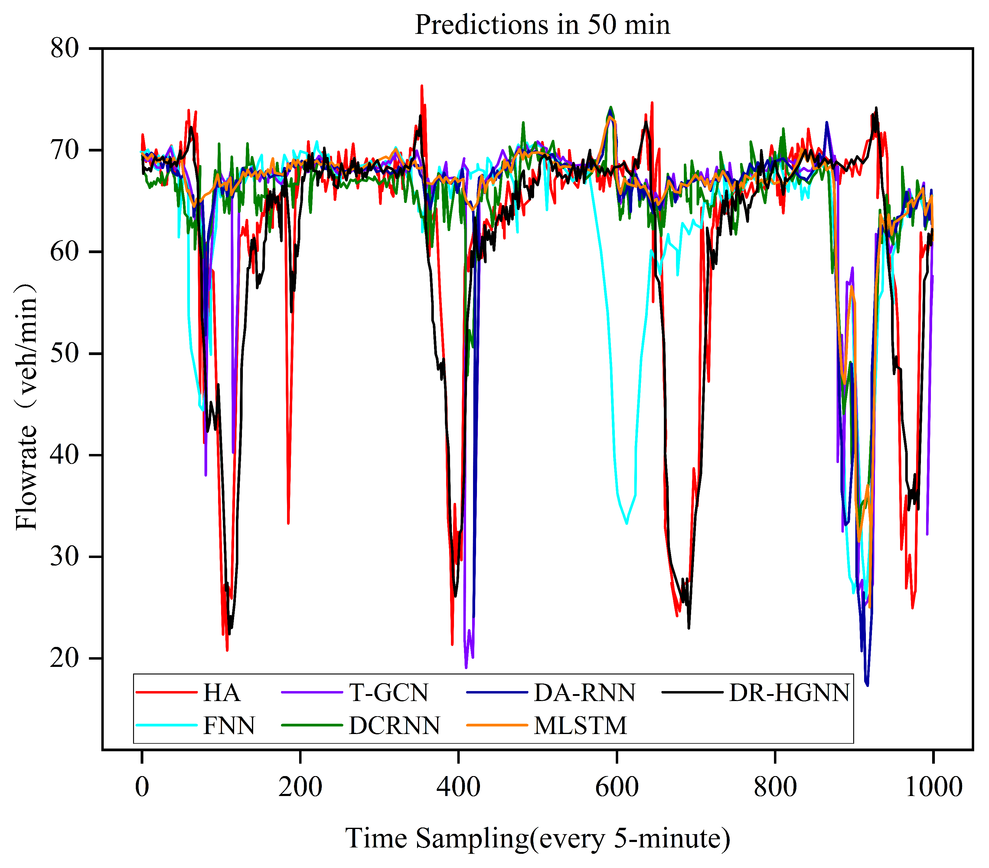
Figure 3 shows the performances of the various models in predicting the next 50 min of the traffic flow in the METR-LA dataset, including the HA, FNN, T-GCN, DCRNN, DA-RNN, MLSTM, and the proposed DR-HGNN model. The horizontal axis represents time-sampling points (every 5 min), and the vertical axis represents the traffic flow (in vehicles per minute).

From the figure, it can be observed that HA (the historical average model) deviates significantly from the actual traffic flow trend, failing to accurately reflect the complex dynamic traffic conditions. The traditional FNN model shows some improvement in relatively stable areas but still exhibits noticeable delays or deviations in areas with rapid traffic changes. Graph-neural-network-based models, such as T-GCNs and DCRNNs, perform more stably, capturing spatial and temporal dependencies to some extent, but still have some errors in regions of sudden change (e.g., at around the 600th time point). In contrast, the proposed DR-HGNN model (black curve) maintains a high degree of consistency with the actual traffic flow throughout the period, especially in areas with sharp fluctuations in traffic levels. The model can quickly capture and adapt to traffic changes. This demonstrates that the DR-HGNN, through dynamic heterogeneous graphs and regional aggregation strategies, effectively enhances its ability to predict complex traffic flow variations.

5.6. Ablation Experiments

To further investigate the impact of each component of the DR-HGNN model on its performance, this study conducts ablation experiments, including the performance after removing the ordinary regional aggregation module (DR-HGNN-w/o-Ordinary Regional Aggregation) and the important regional aggregation module (DR-HGNN-w/o-Important Regional Aggregation), as well as a comparison with the performance of the complete model (DR-HGNN). The ablation experiments are conducted in two datasets (METR-LA and PEMS-BAY), using MAE (mean absolute error) and RMSE (root-mean-square error) as evaluation metrics.

Table 4. Ablation experimental results of the DR-HGNN model.

Model	METR-LA		PEMS-BAY
	MAE	RMSE	MAE	RMSE
DR-HGNN-w/o-Ordinary Regional Aggregation	5.18	5.31	7.48	9.36
DR-HGNN-w/o-Important Regional Aggregation	4.88	5.24	6.07	8.88
DR-HGNN	4.26	5.03	5.32	6.37

presents the results of the ablation experiments for the DR-HGNN model.

From Table 4, it can be observed that after removing the ordinary regional aggregation module, the model’s MAE increases to 5.18 and 7.48, and it’s RMSE increases to 5.31 and 9.36 in the METR-LA and PEMS-BAY datasets, respectively. This indicates that the ordinary regional aggregation module significantly affects the overall performance. On the other hand, the increases in MAE and RMSE are relatively smaller when removing the important regional aggregation module, but this still demonstrates the importance of the key nodal predictions in the important region. The complete model (DR-HGNN) outperforms all the other models in both datasets, validating the complementary and necessary roles of both the ordinary regional and important regional aggregation modules in enhancing the model’s performance.

Therefore, both the ordinary regional aggregation module and the important regional aggregation module make crucial contributions to the model’s performance. The ordinary regional aggregation module has a greater impact on the model’s overall prediction performance, while the important regional aggregation module significantly improves the model’s performance in key areas. The complete DR-HGNN model achieves the best performance in both datasets by integrating the advantages of these two modules, demonstrating the rationality and effectiveness of the proposed model design.

5.7. Complexity Analysis

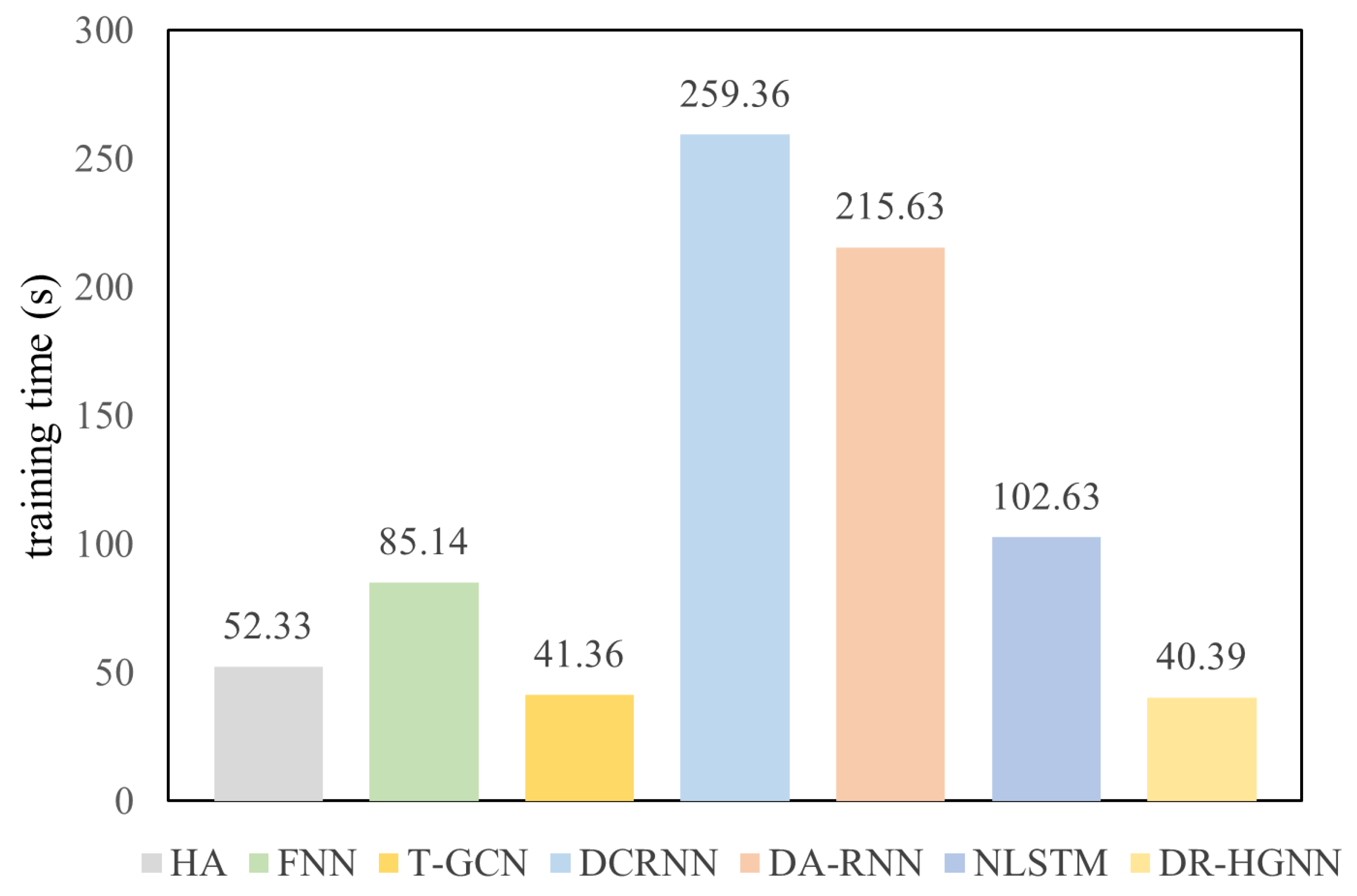
To evaluate the computational efficiency of the proposed model, we compared the average training time per epoch of the DR-HGNN model with those of the six baseline models in the METR-LA dataset, as shown in Figure 4. It can be observed that the training time for the DR-HGNN is 40.39 s, which is the shortest among all the models. In contrast, the training times for the DCRNN and DA-RNN are 259.36 s and 215.63 s, respectively, significantly higher than those of the other models. This indicates that traditional models still have shortcomings in terms of computational complexity and training efficiency. However, the DR-HGNN not only significantly reduces the training time but also maintains strong prediction performance, demonstrating its superiority in dynamic traffic flow prediction tasks.

As shown in

Table 5. The complexities of the different models in the METR-LA dataset.

Model	FLOPs (M)
HA	$3.6\hspace{0.17em}\times \hspace{0.17em}{10}^2$
FNN	$5.3\hspace{0.17em}\times \hspace{0.17em}{10}^3$
T-GCN	$1.0\hspace{0.17em}\times \hspace{0.17em}{10}^4$
DCRNN	$1.3\hspace{0.17em}\times \hspace{0.17em}{10}^2$
DA-RNN	$5.2\hspace{0.17em}\times \hspace{0.17em}{10}^3$
NLSTM	$8.6\hspace{0.17em}\times \hspace{0.17em}{10}^2$
DR-HGNN	$2.4\hspace{0.17em}\times \hspace{0.17em}{10}^3$

, the computational complexity of the DR-HGNN for the METR-LA dataset is $2.4\times {10}^3$ M, which is at a moderate level compared to those of the baseline models. It is significantly lower than those of traditional methods, such as the FNN ($5.3\times {10}^3$ M) and T-GCN ($1.0\times {10}^4$ M), but higher than those of lightweight models, like the DCRNN ($1.3\times {10}^2$ M). This computational overhead mainly arises from its heterogeneous graph structure and dynamic spatiotemporal modeling mechanism, where multi-type nodal relationships and high-order neighborhood aggregation increase the computational burden. However, through optimization strategies, such as sparse graph computation and hierarchical aggregation, the DR-HGNN achieves a 53.8% reduction in the computational complexity compared to that of the DA-RNN ($5.2\times {10}^3$ M), while maintaining strong expressive capability. Although its computational cost is higher than that of the DCRNN, its superior prediction accuracy justifies this increase in the computational complexity, making it suitable for scenarios where higher levels of precision are required.

5.8. Parameter Sensitivity Experiment

This section presents a systematic parameter sensitivity experiment focusing on the nodal division threshold, $ϵ$. The experiment tested the impacts of different $ϵ$ values on the model’s performance, using the METR-LA and PEMS-BAY benchmark datasets. The results show that the setting of the $ϵ$ parameter has a significant impact on the prediction accuracy, with the optimal value consistently at around 50%.

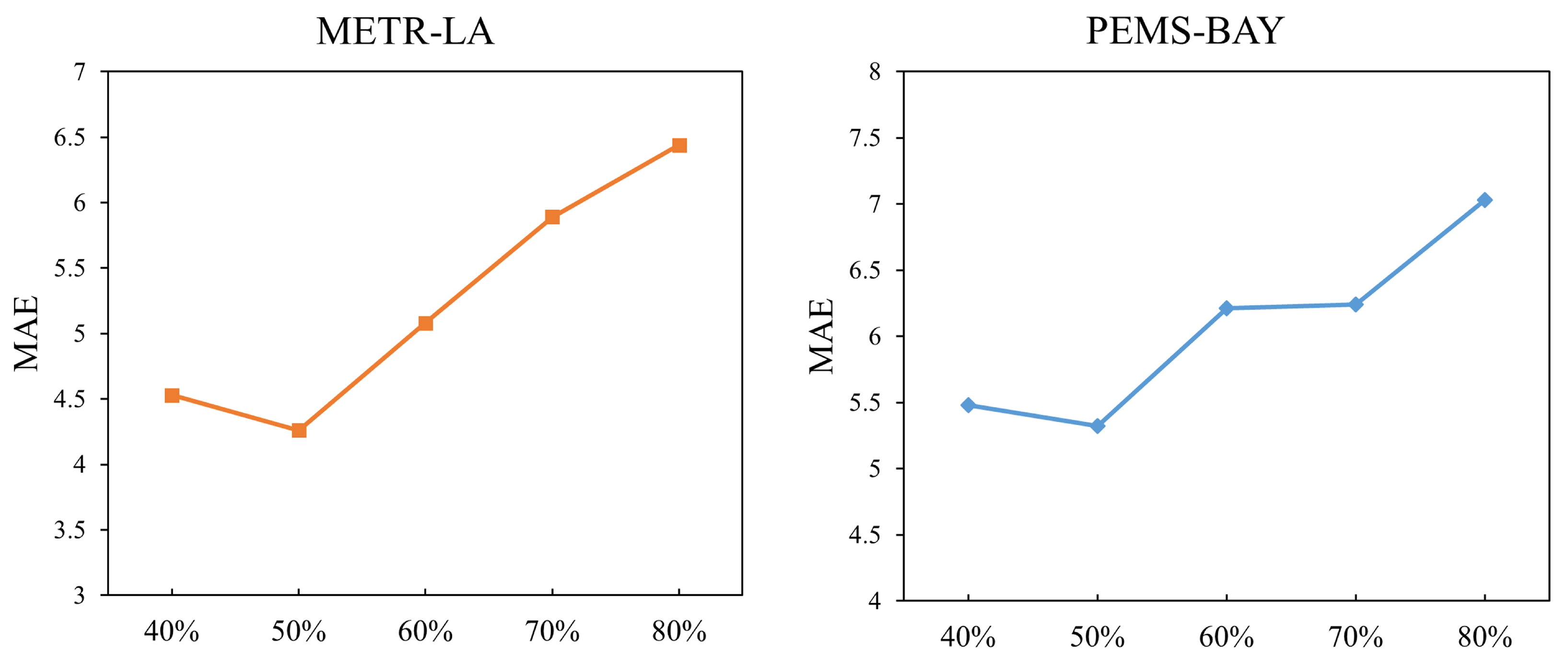
As shown in Figure 5, similar patterns of MAE variation were observed in both datasets. When $ϵ$ increased from 40% to 50%, the model’s performance improved significantly: the MAE of the METR-LA dataset decreased by 5.96%, and the PEMS-BAY dataset’s MAE decreased by 2.92%. This indicates that appropriately increasing the proportion of ordinary nodes helps the model to learn more representative traffic patterns. However, when $ϵ$ exceeds 50%, the MAEs of both datasets show a monotonously increasing trend, suggesting that too many ordinary nodes dilute the influence of important nodal features.

It is worth noting that the sensitivity to $ϵ$ changes varies across datasets. The METR-LA dataset demonstrated a stronger sensitivity, with a maximum fluctuation of 42.2%, reflecting the urban road network structure’s strong dependence on the nodal division. In contrast, the PEMS-BAY dataset reached a performance plateau in the 60–70% range, which may be because of its more uniform traffic flow distribution characteristics.

6. Conclusions

We propose a dynamic regional-aggregation-based heterogeneous graph neural network (DR-HGNN) for traffic flow prediction. This model effectively captures the spatiotemporal dependencies of traffic data by constructing a heterogeneous graph of the traffic network and incorporating a regional aggregation strategy. In ordinary regions, the model aggregates features from the second-order neighbors of the target nodes, while in important regions, the model aggregates features from the third-order neighbors, fully exploring the differences between ordinary and important regions. Additionally, attention mechanisms are used to fuse the aggregated features, providing more accurate traffic predictions. Experiments on the METR-LA and PEMS-BAY public datasets demonstrate that our model significantly outperforms existing baseline methods. Ablation studies further validate the critical roles of the ordinary and important regional aggregation modules in enhancing the model’s performance. This indicates that region-based heterogeneous graph modeling can better capture the dynamic spatial–temporal dependencies in different regions of the traffic network. Future research will further explore the applicability of dynamic heterogeneous graph neural networks in more complex scenarios, including the consideration of various external factors (e.g., weather and events) that affect the traffic flow, and optimizing the model to adapt to larger-scale and higher-frequency traffic data, thereby improving the accuracy and timeliness of traffic predictions.

However, this study still has some limitations. First, the model’s division of regional importance still relies on prior knowledge and has not fully achieved adaptive dynamic regional identification. Second, the model’s robustness needs further improvement when handling abnormal traffic conditions, such as extreme weather or emergency events. Finally, as the road network’s scale increases, the computational complexity caused by higher-order neighbor aggregation may affect the real-time performance of the model. Future research will focus on addressing these issues by introducing an adaptive regional division mechanism, enhancing anomaly detection capabilities, and optimizing computational efficiency to further improve the model’s applicability in complex real-world scenarios. Additionally, exploring multimodal data fusion (such as weather, POIs, and other external factors) will be an important research direction.