Detecting Clinical Risk Shift Through log–logistic Hazard Change-Point Model

Abstract

The change–point problem is about identifying when a pattern or trend shifts in time–ordered data. In survival analysis, change–point detection focuses on identifying alterations in the distribution of time–to–event data, which may be subject to censoring or truncation. In this paper, we introduce a change–point in the hazard rate of the log–logistic distribution. The log–logistic distribution is a flexible probability distribution used in survival analysis, reliability engineering, and economics. It is particularly useful for modeling time–to–event data exhibiting decreasing hazard rates. We estimate the parameters of the proposed change–point model using profile maximum likelihood estimation. We also carry out a simulation study and Bayesian analysis using the Metropolis–Hastings algorithm to study the properties of the proposed estimators. The proposed log–logistic change–point model is applied to survival data from kidney catheter patients and acute myeloid leukemia (AML) cases. A late change–point with a decreasing scale parameter in the catheter data reflects an abrupt increase in risk due to delayed complications, whereas an early change–point with an increasing scale parameter in AML indicates high early mortality followed by slower hazard progression in survivors. We find that the log–logistic change–point model performs better in comparison to the existing change–point models.

1. Introduction and Background

In survival analysis, the log–logistic distribution serves as an alternative to the more commonly used Weibull and log–normal distributions, offering an advantage when the data display a decreasing hazard rate. The probability density function (PDF) and the hazard function of the log–logistic distribution are, respectively, given by the following:

$$f(x;\alpha )={\displaystyle \frac{\alpha }{{(\alpha +x)}^2}},x>0$$

$$h(x;\alpha )={\displaystyle \frac{\alpha }{\alpha +x}},x>0$$

(1)

where $\alpha >0$.

The log–logistic distribution is widely used in survival analysis due to its ability to model decreasing hazard rates, making it suitable where the risk of an event declines over time. Several studies have contributed to the application of the log–logistic model. To mention a few, Gupta et al. (1999) [1] considered the log–logistic model to analyze lung cancer data and evaluated the confidence intervals for both parameters and the critical points. They also computed the mean residual life function and maximum likelihood estimators, which were found to be unique for both parameters. Bennett (1983) [2] considered a log–logistic regression model by equating one parameter of the distribution with a linear function of the covariates, which was a special case of the proportional odds model, and tested it on patients with advanced inoperable lung cancer. He fitted the data using the Generalized Linear Interactive Modeling software and found that the model captured the general shape of the data very well. Muse et al. (2021) [3] comprehensively reviewed the log–logistic distribution and its generalizations, highlighting its mathematical properties, applications, and advancements in statistical modeling.

Apart from analyzing survival data, the log–logistic distribution has gained increasing traction in various fields such as economics, medical sciences, hydrology, and social sciences. Lemonte (2014) [4] incorporated the beta distribution as a weight function, allowing for greater adaptability in fitting real–world data. Ashkar and Mahdi (2006) [5] investigated the use of the generalized moment (GM) method for estimating parameters and quantiles in the two–parameter log–logistic (LL2) distribution. They compared the GM method with other common estimation techniques, including the generalized probability–weighted moments and the maximum likelihood method, and observed that the GM method provided more accurate parameter estimates in the LL2 case when moment orders were appropriately selected. Shoukri, Mian, and Tracy (1988) [6] examined the sampling properties of the estimators for the log–logistic distribution, focusing on its application to Canadian precipitation data. They compared the following two estimation methods: probability–weighted moments and maximum likelihood estimation. Their findings confirmed that the log–logistic distribution provided an excellent fit for various meteorological datasets, making it a valuable tool in hydrology and climatology. De Santana et al. (2012) [7] introduced the Kumaraswamy–log–logistic distribution, a generalization of the log–logistic distribution designed to provide greater flexibility in modeling lifetime and survival data. Ramos et al. (2013) [8] introduced the Zografos–Balakrishnan–log–logistic distribution, an extension of the traditional log–logistic model. This distribution accommodated various hazard function shapes, enhancing flexibility in survival analysis. Alfaer et al. (2021) [9] introduced the extended log–logistic (Ex–LL) distribution, a flexible extension of the traditional log–logistic model designed to better capture actuarial and engineering risk data, particularly those with heavy–tailed distributions. Felipe et al. (2023) [10] proposed a robust estimation approach for the log–logistic distribution using minimum density power divergence estimators (MDPDEs) to address the limitations of traditional methods in the presence of outliers. The study demonstrated, through simulation and real data, that the MDPDEs offered a favorable balance between efficiency and robustness, making them suitable for practical survival analysis. Gaire and Gurung (2024) [11] introduced a new four–parameter log–logistic distribution based on the Rayleigh distribution. They carried out two methods of estimation and derived the statistical properties of the estimators, such as moments, survival function, etc. They applied it on two real–world datasets and found that the proposed model performed better than some select probability models.

Change–Point Problems in Survival Analysis

The problem of change–points in survival analysis has been a topic of interest for researchers in the past few decades. Matthews and Farewell (1982) [12] were among the first to consider change–point detection in hazard functions. Chang, Chen, and Hsiung (1994) [13] developed estimation methods for change–point hazard rate models under random censorship. Gijbels and Gürler (2003) [14] proposed a model incorporating a hazard jump at a specific time point and estimated the unknown parameters using maximum likelihood estimation, a least squares estimator, and the cumulative hazard–based approach introduced by Chang, Chen and Hsiung. Goodman, Li, and Tiwari (2011) [15] developed methods to detect multiple change–points in piecewise constant hazard functions. Williams and Kim (2013) [16] developed a Weibull hazard model considering Type–I censoring and staggered entry and studied the applicability of the model through a data on chronic granulomatous disease. Joshi et al. (2017) [17] proposed the Lindley hazard change–point model, estimating that the risk of death from a bone marrow transplant in patients with acute lymphoblastic leukemia significantly decreases after certain time. Palmeros et al. (2018) [18] considered a Weibull hazard regression model in the presence of covariates and censored observations. They estimated the parameters using maximum likelihood estimation and Monte Carlo simulation and applied the model on data regarding chronic granulomatous disease. Joshi and Rattihalli (2019) [19] proposed a general hazard regression change–point model where the effect of covariates on lifetime begins after the change–point. The Exponential–Lindley hazard change–point model was introduced by Joshi and Rattihalli (2020), ref. [20] where the failure rate remained constant before and after the change–point, following a Lindley distribution failure rate. Gierz and Park (2022) [21] proposed a sequential testing approach for detecting multiple change–points in a Weibull accelerated failure time (AFT) model and conducted a simulation study to show that the proposed method detected change–points and estimated the model quite accurately.

Despite the log–logistic model being a popular survival model, its scope in the field of change–point analysis is unattempted. Thus, in this paper, we aim to achieve the following:

• Introduce a novel hazard change–point model, namely the log–logistic hazard change–point model;
• Estimate the model parameters using the profile maximum likelihood estimation method and the Bayesian method, as well as compare the results for varying sample sizes and censoring levels;
• Show the suitability of the model to detect a change–point in two real–world datasets.

The article is organized as follows: After an introduction and background in Section 1, the proposed change–point model is introduced in Section 2. In Section 3, parameter estimation using the profile maximum likelihood estimation procedure is shown followed by a simulation study in Section 4. We also evaluate the performance of the estimators through a Bayesian analysis, carried out in Section 5. In Section 6, a real–life data analysis is performed using the proposed change–point model. Lastly, Section 7 discusses the findings and future works.

2. log–logistic Hazard Change–Point Model for Survival Analysis

Let T be a survival time variable with a hazard function given by Equation (1). Suppose after a certain point in time, say $\tau$, ${\alpha }_1$ changes to ${\alpha }_2$. The hazard model under this setup is now given by the following equation:

$$h\left(t\right)=\left\{\begin{array}{cc}{\displaystyle \frac{1}{{\alpha }_1+t}},\hfill & 0⩽t⩽\tau ,\hfill \\ \\ {\displaystyle \frac{1}{{\alpha }_2+t}}\hfill & t>\tau ,\hfill \end{array}\right.$$

where ${\alpha }_1>0$ and ${\alpha }_2+\tau >0$. It can be seen that if ${\alpha }_1$ < (>)${\alpha }_2$, then the hazard function beyond the change–point is at lower (higher) level than the hazard function below the change–point. It can also be noted that both the hazard functions are decreasing in X (Figure 1).

The PDF and the survival function corresponding to the above model are as follows

$$f\left(t\right)=\left\{\begin{array}{cc}{\displaystyle \frac{{\alpha }_1}{{({\alpha }_1+t)}^2}},\hfill & 0⩽t⩽\tau ,\hfill \\ \\ {\displaystyle \frac{{\alpha }_1({\alpha }_2+\tau )}{({\alpha }_1+\tau ){({\alpha }_2+t)}^2}}\hfill & t>\tau ,\hfill \end{array}\right.$$

and

$$S\left(t\right)=\left\{\begin{array}{cc}{\displaystyle \frac{{\alpha }_1}{{\alpha }_1+t}},\hfill & 0⩽t⩽\tau ,\hfill \\ \\ {\displaystyle \frac{{\alpha }_1({\alpha }_2+\tau )}{({\alpha }_1+\tau )({\alpha }_2+t)}}\hfill & t>\tau .\hfill \end{array}\right.$$

(2)

where we have three parameters—${\alpha }_1$, ${\alpha }_2$, and $\tau$—to be estimated. In the next section, we discuss the profile maximum likelihood estimation (PMLE) method.

3. Parameter Estimation Using PMLE

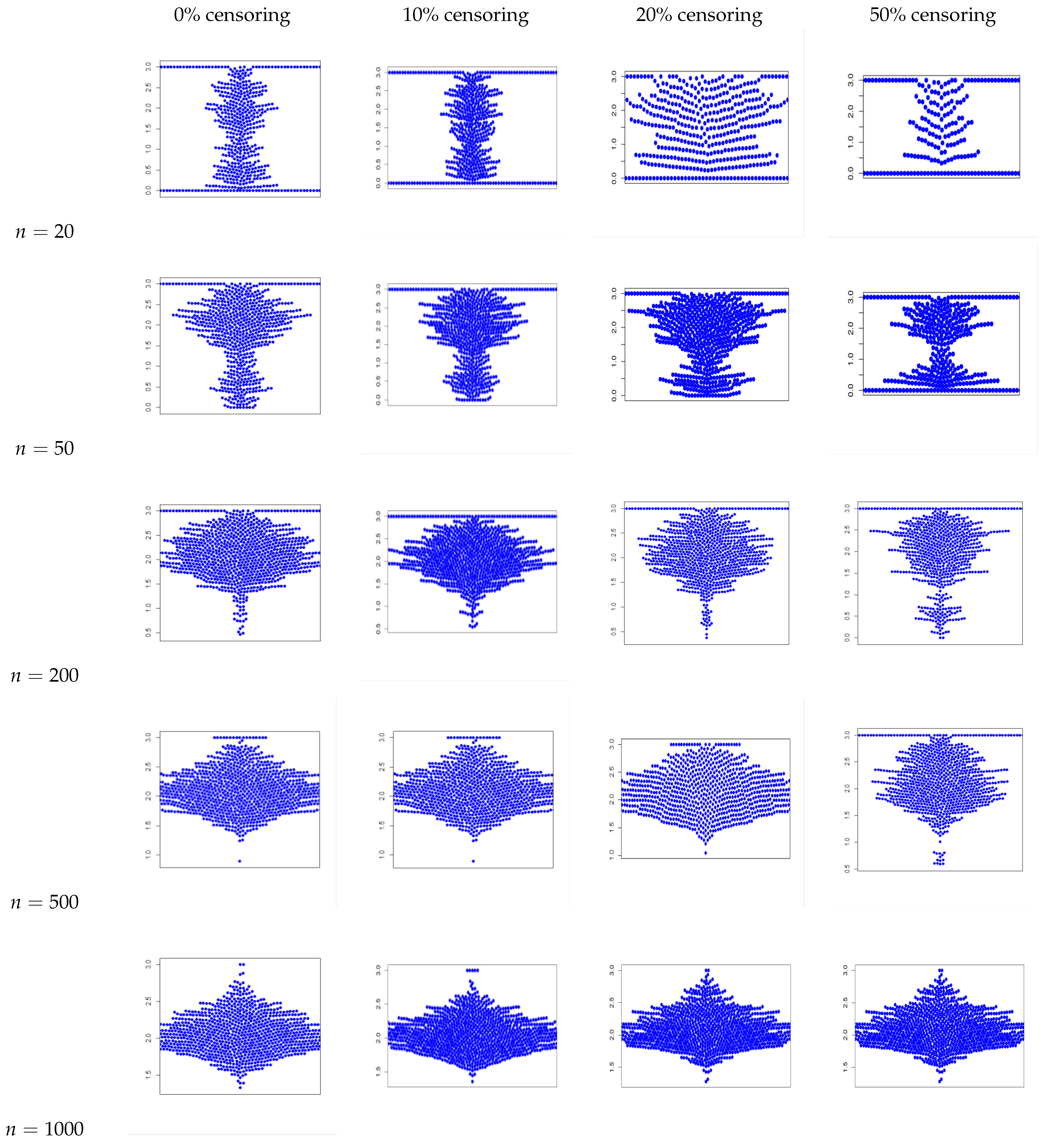
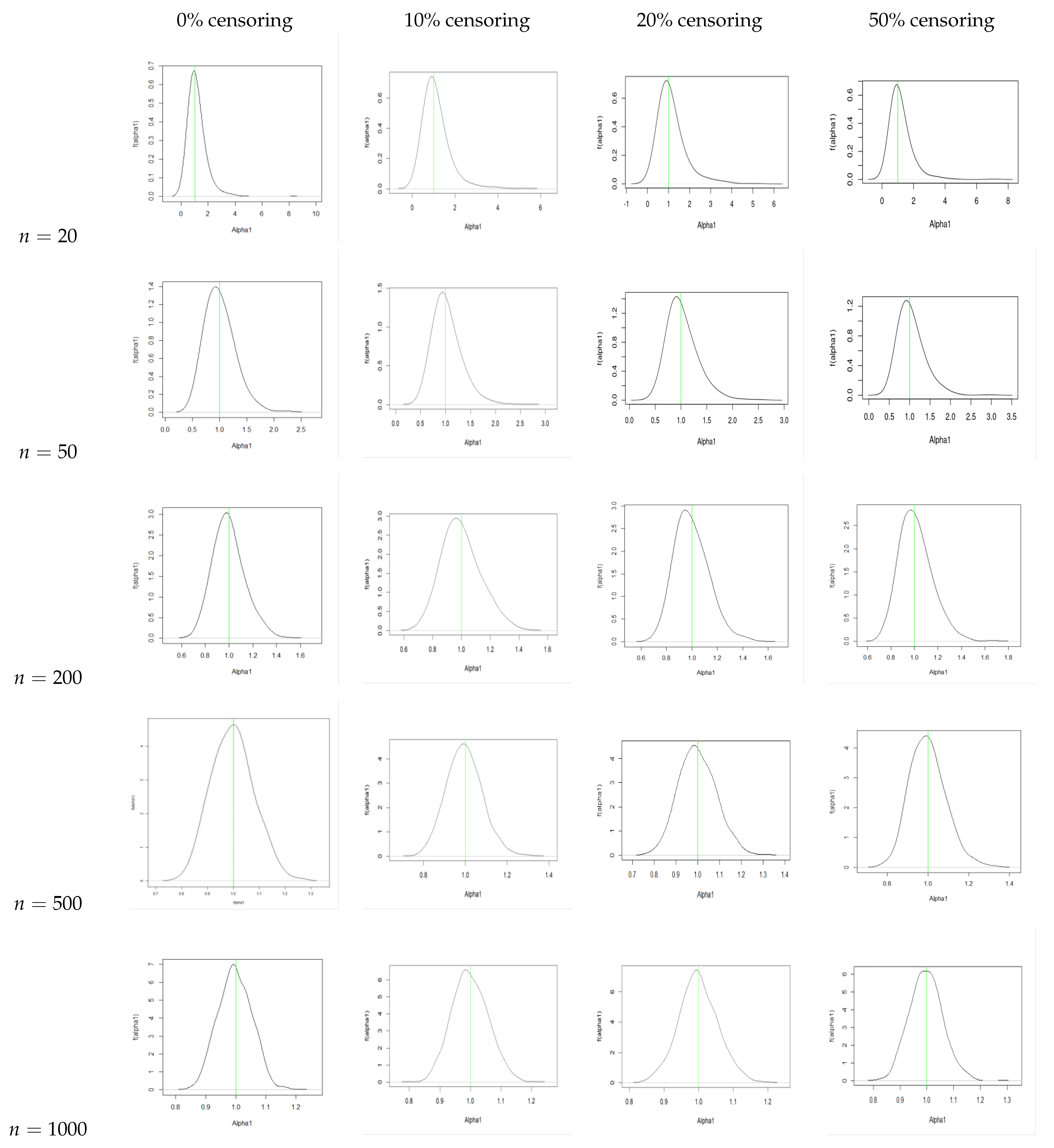
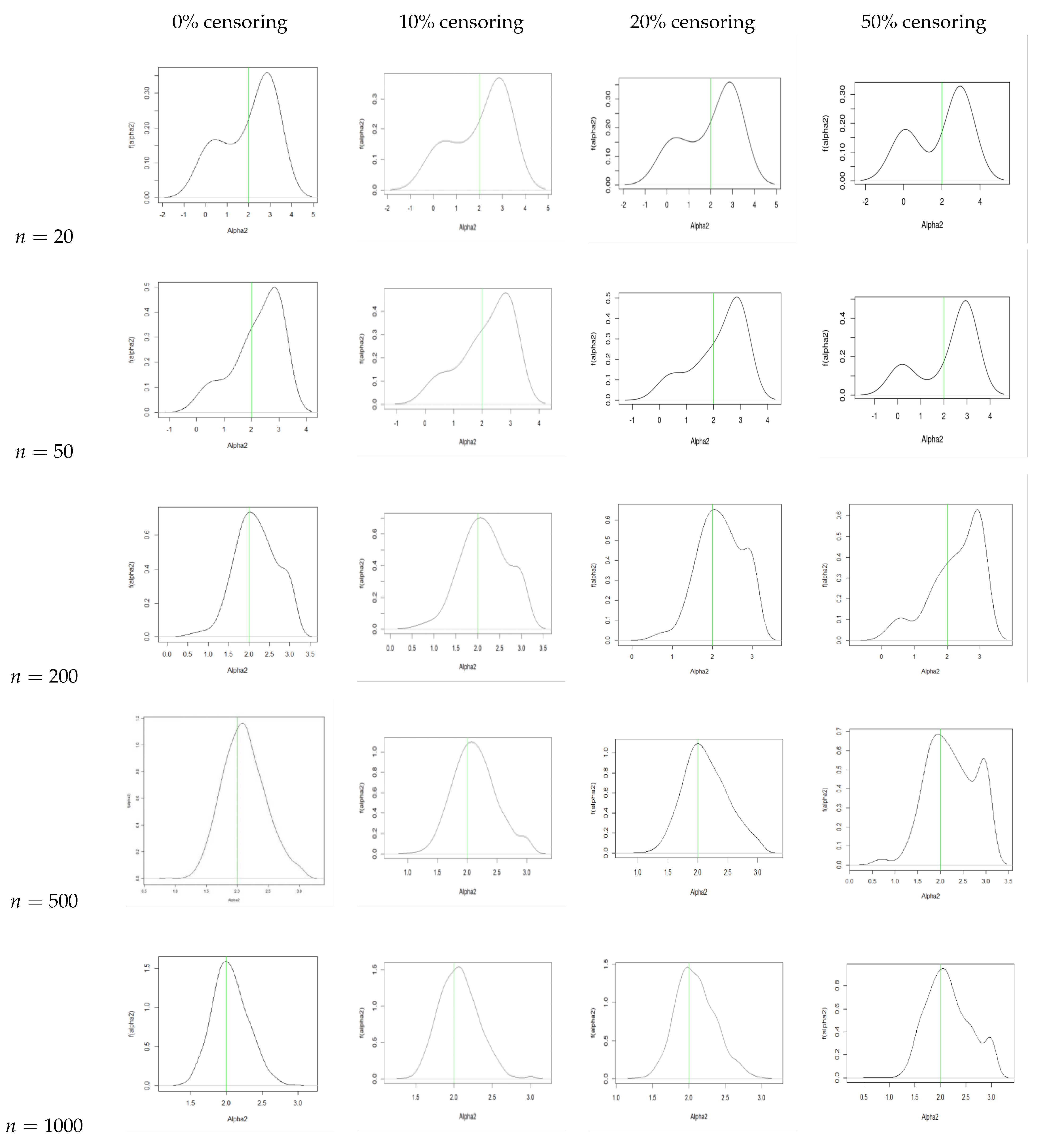
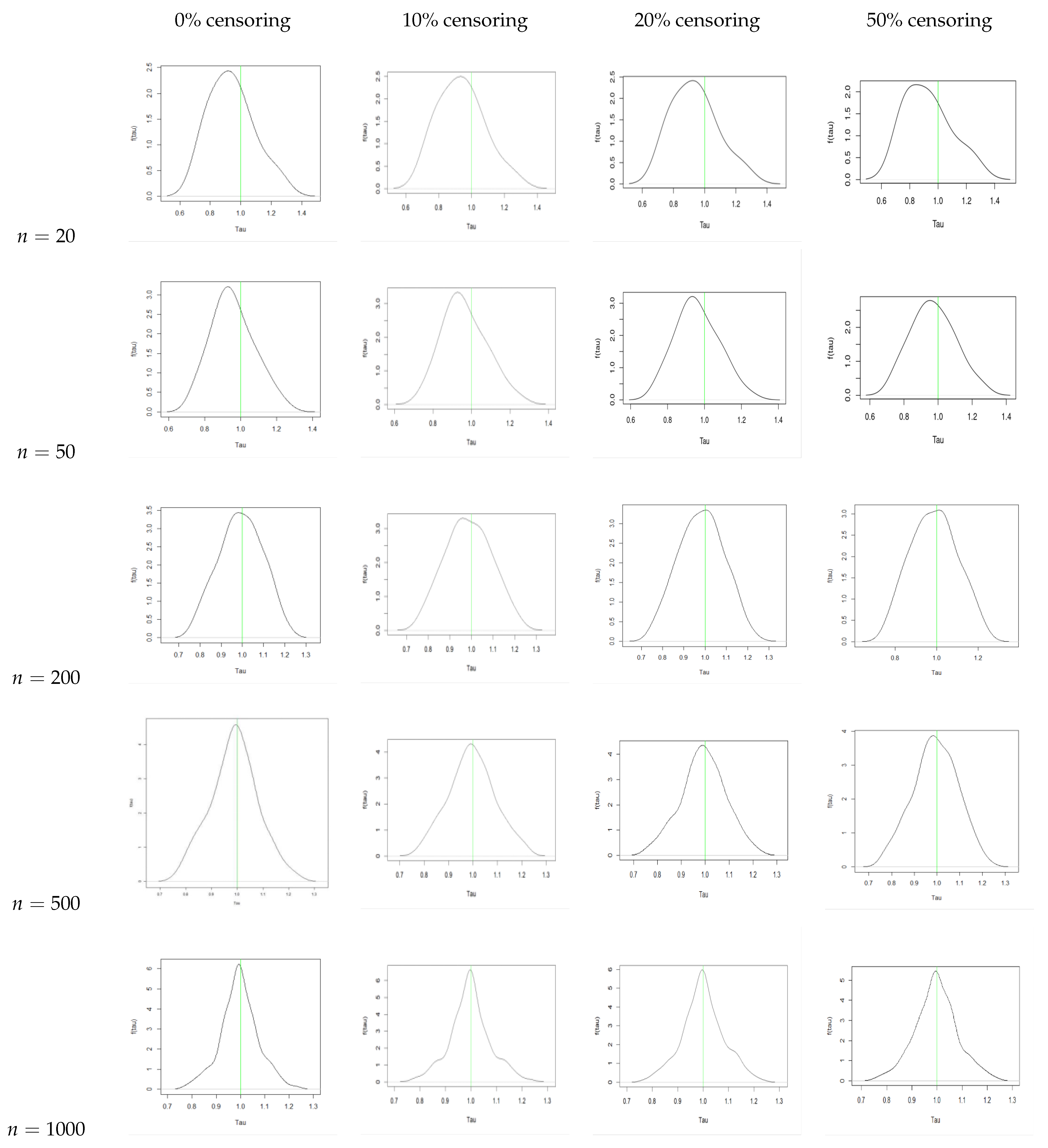
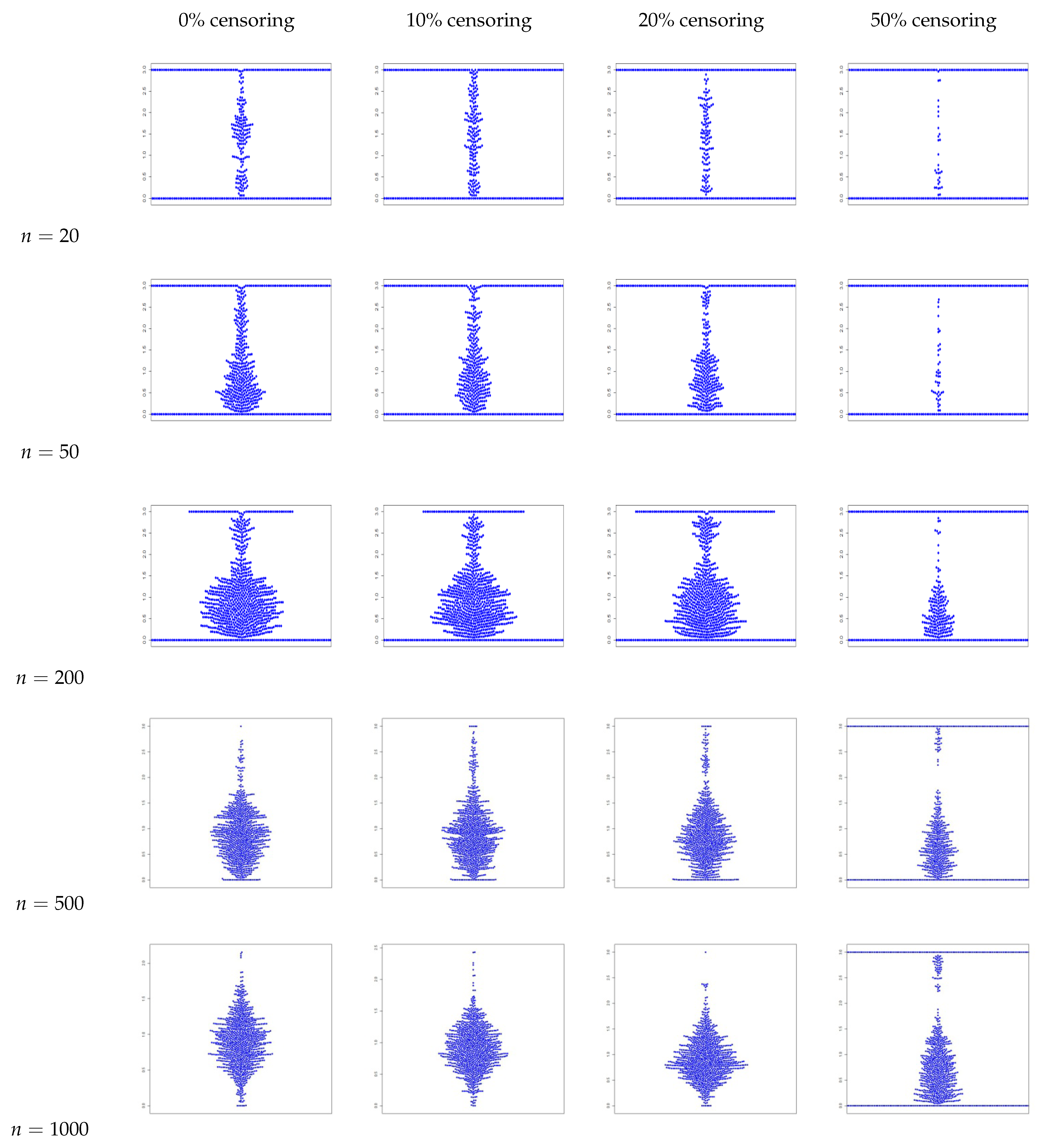
To estimate the parameters, we opt for PMLE; however, one may use any command based approach of multi parameter estimation in R or any other suitable platform.

We shall consider random right censoring, i.e., instead of observing the survival time $T_i$, we observe a pair ($T_i$, $C_i$) ($C_i$ is the right censored observations) and a censoring indicator ${ϵ}_i$, where ${ϵ}_i=1$ for an uncensored observation, and 0 for a censored observation. The study variable now becomes $X_i=$min$(T_i,C_i)$.

With the assumption of independent censoring, the likelihood function for the pair ($X_i$, ${ϵ}_i$) is expressed as follows:

$$\begin{array}{ccc}\hfill L({\alpha }_1,{\alpha }_2,\tau |\underline{x})& \propto & \prod _{i=1}^n{\left(f\left(x_i\right)\right)}^{{ϵ}_i}\prod _{i=1}^n{\left(S\left(x_i\right)\right)}^{(1-{ϵ}_i)}.\hfill \end{array}$$

where n is the total number of observations in the data. In the presence of a change–point, the likelihood changes to the following:

$$\begin{array}{ccc}\hfill L({\alpha }_1,{\alpha }_2,\tau |\underline{x})& \propto & \prod _{i=1}^n{\left(f\left(x_i\right)\right)}^{I(X_i⩽\tau ){ϵ}_i}\prod _{i=1}^n{\left(S\left(x_i\right)\right)}^{I(X_i⩽\tau )(1-{ϵ}_i)}\hfill \\ \hfill & & \prod _{i=1}^n{\left(f\left(x_i\right)\right)}^{I(X_i>\tau ){ϵ}_i}\prod _{i=1}^n{\left(S\left(x_i\right)\right)}^{I(X_i>\tau )(1-{ϵ}_i),}\hfill \end{array}$$

where $I_{[0,\tau ]}\left(X_i\right)$ is the indicator function. Substituting the values of $f\left(x\right)$ and $S\left(x\right)$ for the proposed log–logistic model, we obtain the likelihood function as follows:

$$\begin{array}{ccc}\hfill L({\alpha }_1,{\alpha }_2,\tau |\underline{x})& \propto & \prod _{i=1}^n{\left({\displaystyle \frac{{\alpha }_1}{{({\alpha }_1+x_i)}^2}}\right)}^{I(X_i⩽\tau ){ϵ}_i}\prod _{i=1}^n{\left({\displaystyle \frac{{\alpha }_1}{{\alpha }_1+x_i}}\right)}^{I(X_i⩽\tau )(1-{ϵ}_i)}\hfill \\ \hfill & & \prod _{i=1}^n{\left({\displaystyle \frac{{\alpha }_1({\alpha }_2+\tau )}{({\alpha }_1+\tau ){({\alpha }_2+x_i)}^2}}\right)}^{I(X_i>\tau ){ϵ}_i}\prod _{i=1}^n{\left({\displaystyle \frac{{\alpha }_1({\alpha }_2+\tau )}{({\alpha }_1+\tau )({\alpha }_2+x_i)}}\right)}^{I(X_i>\tau )(1-{ϵ}_i)}.\hfill \end{array}$$

The log-likelihood function corresponding to the above expression is as follows:

$$\begin{array}{ccc}\hfill logL({\alpha }_1,{\alpha }_2,\tau |\underline{x})& \propto & \sum _{i=1}^n{ϵ}_{i}I(X_i⩽\tau )log\left({\displaystyle \frac{{\alpha }_1}{{({\alpha }_1+x_i)}^2}}\right)+\sum _{i=1}^n(1-{ϵ}_i)I(X_i⩽\tau )log\left({\displaystyle \frac{{\alpha }_1}{{\alpha }_1+x_i}}\right)\hfill \\ & & +\sum _{i=1}^n{ϵ}_{i}I(X_i>\tau )log\left({\displaystyle \frac{{\alpha }_1({\alpha }_2+\tau )}{({\alpha }_1+\tau ){({\alpha }_2+x_i)}^2}}\right)+\sum _{i=1}^n(1-{ϵ}_i)I(X_i>\tau )log\left({\displaystyle \frac{{\alpha }_1({\alpha }_2+\tau )}{({\alpha }_1+\tau )({\alpha }_2+x_i)}}\right).\hfill \end{array}$$

Let $n_u$ be the total number of uncensored observations in the data. Let $u\left(\tau \right)={\sum }_{i=1}^{n}I(X_i⩽\tau ){ϵ}_i$ and $c\left(\tau \right)={\sum }_{i=1}^{n}I(T_i⩽\tau )(1-{ϵ}_i)$ be the number of uncensored and censored observations by time $\tau$, respectively. The log-likelihood function can be further simplified as follows:

$$\begin{array}{c}\hfill logL({\alpha }_1,{\alpha }_2,\tau |\underline{x})\propto nlog{\alpha }_1-2\sum _{i=1}^n{ϵ}_{i}I(X_i\le \tau )log(x_i+{\alpha }_1)-\sum _{i=1}^n(1-{ϵ}_i)I(X_i\le \tau )log(x_i+{\alpha }_1)\\ \hspace{1em}\hspace{1em}-(n-u\left(\tau \right)-c\left(\tau \right))\left[log({\alpha }_1+\tau )-log({\alpha }_2+\tau )\right]-2\sum _{i=1}^n{ϵ}_{i}I(X_i>\tau )log(x_i+{\alpha }_2)\hfill \\ \hspace{1em}\hspace{1em}-\sum _{i=1}^n(1-{ϵ}_i)I(X_i>\tau )log(x_i+{\alpha }_2)\hfill \end{array}$$

Let $X_{\left(i\right)}$ be the order statistics corresponding to $X_i$, and ${ϵ}_{\left(i\right)}$ be the corresponding censoring indicator. For estimating ${\alpha }_1,{\alpha }_2$ and $\tau$, we assume that $\tau (=\tilde{\tau })$ is known. We consider $\tilde{\tau }$ to be the mid-point of each interval in all the $(n-1)$ intervals $[X_{\left(j\right)},X_{(j+1)}]$, $j=1,2,\cdots ,(n-1)$. The confined log-likelihood is given as follows:

$$\begin{array}{c}\hfill logL({\alpha }_1,{\alpha }_2,\tilde{\tau }|\underline{x})\propto nlog{\alpha }_1-2\sum _{i=1}^n{ϵ}_{\left(i\right)}I(X_{\left(i\right)}\le \tilde{\tau })log(x_{\left(i\right)}+{\alpha }_1)-\sum _{i=1}^n(1-{ϵ}_{\left(i\right)})I(X_{\left(i\right)}\le \tilde{\tau })log(x_{\left(i\right)}+{\alpha }_1)\\ \hspace{1em}\hspace{1em}-(n-u\left(\tilde{\tau }\right)-c\left(\tilde{\tau }\right))\left[log({\alpha }_1+\tilde{\tau })-log({\alpha }_2+\tilde{\tau })\right]-2\sum _{i=1}^n{ϵ}_{\left(i\right)}I(X_{\left(i\right)}>\tilde{\tau })log(x_{\left(i\right)}+{\alpha }_2)\hfill \\ \hspace{1em}\hspace{1em}-\sum _{i=1}^n(1-{ϵ}_{\left(i\right)})I(X_{\left(i\right)}>\tilde{\tau })log(x_{\left(i\right)}+{\alpha }_2)\hfill \end{array}$$

(3)

By applying the principle of maximum likelihood (ML) estimation and taking the partial derivatives of the simplified log-likelihood with respect to ${\alpha }_1$ and ${\alpha }_2$, we get the following equations:

$${\displaystyle \frac{\partial logL({\alpha }_1,{\alpha }_2,\tau |\underline{x})}{\partial {\alpha }_1}}={\displaystyle \frac{n}{{\alpha }_1}}-2\sum _{i=1}^n{\displaystyle \frac{{ϵ}_{i}I(X_i⩽\tau )}{{\alpha }_1+x_i}}-\sum _{i=1}^n{\displaystyle \frac{(1-{ϵ}_i)I(X_i⩽\tau )}{{\alpha }_1+x_i}}-{\displaystyle \frac{n-u\left(\tau \right)-c\left(\tau \right)}{{\alpha }_1+\tau }},$$

and

$${\displaystyle \frac{\partial logL({\alpha }_1,{\alpha }_2,\tau |\underline{x})}{\partial {\alpha }_2}}={\displaystyle \frac{n_u-u\left(\tau \right)-c\left(\tau \right)}{{\alpha }_2+\tau }}-2\sum _{i=1}^n{\displaystyle \frac{{ϵ}_{i}I(X_i>\tau )}{{\alpha }_2+x_i}}-\sum _{i=1}^n{\displaystyle \frac{(1-{ϵ}_i)I(X_i>\tau )}{{\alpha }_2+x_i}}.$$

The above likelihood equations cannot be solved analytically for both ${\alpha }_1$ and ${\alpha }_2$, therefore we employ numerical methods of estimation using the nlm() and the optimize() function in R [22]. To estimate ${\alpha }_1$, we consider ${\alpha }_2$ to be known (nuisance parameter). The initial value of ${\alpha }_2$ is taken to be the one used in the data simulation. By maximizing Equation (3) with respect to ${\alpha }_1$, using the nlm() function and the same seed value of ${\alpha }_1$ as that used in the data simulation, we obtain the PML estimate of ${\alpha }_1$ for the $jth$ interval, denoted as ${\widehat{{\alpha }_1}}_j$. Then, by replacing ${\alpha }_1$ with ${\widehat{{\alpha }_1}}_j$ in (3) and maximizing it for ${\alpha }_2$ using the optimize() function, as well as considering the interval for ${\alpha }_2$ such that the estimated value falls in the given interval, (0,3) yields the PML estimate of ${\alpha }_2$ for the $jth$ interval, denoted as ${\widehat{{\alpha }_2}}_j$. Substituting the values of ${\widehat{{\alpha }_1}}_j$ and ${\widehat{{\alpha }_2}}_j$ obtained in (3) and maximizing the function over [$X_{\left(1\right)},X_{\left(n\right)}$] will give us the estimate ${\widehat{\tau }}_j$. Proceeding iteratively, we obtain the estimates ${\widehat{{\alpha }_1}}_j,{\widehat{{\alpha }_2}}_j,$ and ${\widehat{\tau }}_j$ for all the intervals.

We compute the log-likelihood $log{L}_j({\widehat{{\alpha }_1}}_j,{\widehat{{\alpha }_2}}_j,{\widehat{\tau }}_j),j=1,2,\cdots ,(n-1)$. Suppose the maximum value of the likelihood is obtained at index $\overline{j}$. The estimates of $({\widehat{{\alpha }_1}}_j,{\widehat{{\alpha }_2}}_j,{\widehat{\tau }}_j)$ corresponding to $\overline{j}$ will provide us with the PML estimates of the parameters, i.e., ${\widehat{{\alpha }_1}}_{\overline{j}},{\widehat{{\alpha }_2}}_{\overline{j}},{\widehat{\tau }}_{\overline{j}}$.

4. Simulation Study

In order to simulate data for our analysis, we use the inverse cumulative distribution function (CDF) technique. For this purpose, we obtain a random sample from a standard rectangular distribution $U(0,1)$ of the same size as our data. If our distribution function is denoted by $F\left(x\right)$, equating it with the random uniform sample $F\left(x\right)=u$ previously generated will yield the required data $x=F^{-1}\left(u\right)$ for a fixed value of $({\alpha }_1,{\alpha }_2,\tau )$.

The distribution function for the model proposed in Equation (2) is as follows:

$${\displaystyle F\left(x\right)=1-S\left(x\right)=\left\{\begin{array}{cc}\frac{x}{{\alpha }_1+x},\hfill & 0⩽x⩽\tau ,\hfill \\ \frac{({\alpha }_1+\tau )x+({\alpha }_2-{\alpha }_1)\tau }{({\alpha }_1+\tau )({\alpha }_2+x)},\hfill & x>\tau .\hfill \end{array}\right.}$$

For the change–point $\tau$, the corresponding uniform number will be $u_0=F\left(\tau \right)={\displaystyle \frac{\tau }{{\alpha }_1+\tau }}$. The generated sample is thus given by the following:

$${\displaystyle x=F^{-1}\left(u\right)=\left\{\begin{array}{cc}\frac{u{\alpha }_1}{1-u},\hfill & 0\le u\le u_0,\hfill \\ \frac{1}{1-u}\left(\frac{{\alpha }_2+\tau }{{\alpha }_1+\tau }\right){\alpha }_1-{\alpha }_2+{\alpha }_{2}u,\hfill & u_0<u\le 1.\hfill \end{array}\right.}$$

To check how well the proposed estimators work, we use PMLE. We use the following two sets of parameters for the estimation: (${\alpha }_1$ = 1, ${\alpha }_2$ = 2, $\tau$ = 1) and (${\alpha }_1$ = 2, ${\alpha }_2$ = 1, $\tau$ = 3). The estimation procedure is repeated 1000 times to ensure the reliability of the results. For each simulation run, we generate random samples from the log–logistic distribution with predefined parameters. We test for different sample sizes (n), 20, 50, 200, 500, and 1000, to see how the estimators perform under four levels of right-censoring, including 0%, 10%, 20%, and 50%. To assess the performance of the proposed estimators, we calculate bias and mean square error (MSE) and present them in

Table 1. Mean estimated value (MEV), bias, and MSE of proposed model based on 1000 iterations for ${\alpha }_1$ = 1, ${\alpha }_2$ = 2, $\tau$ = 1.

		${\mathit{\alpha }}_1$			${\mathit{\alpha }}_2$			$\mathit{\tau }$
Censoring	$\mathit{n}$	MEV	Bias	MSE	MEV	Bias	MSE	MEV	Bias	MSE
0%	20	1.1166	0.1166	0.3426	2.1987	0.1987	1.2613	0.9383	−0.0616	0.0225
	50	1.0076	0.0076	0.0769	2.1770	0.1770	0.7837	0.9565	−0.0434	0.0156
	200	0.9972	−0.0028	0.0179	2.1079	0.1079	0.2890	0.9887	−0.0112	0.0105
	500	0.9973	−0.0027	0.0067	1.9134	−0.0865	0.1290	0.9922	−0.0077	0.0088
	1000	0.9981	−0.0018	0.0031	2.0605	0.0605	0.0684	0.9960	−0.0039	0.0062
10%	20	1.1175	0.1175	0.4022	2.1609	0.1609	1.2923	0.9388	−0.0611	0.0222
	50	1.0312	0.0312	0.0835	2.1525	0.1525	0.8102	0.9640	−0.0359	0.0140
	200	0.9953	−0.0046	0.0179	2.1294	0.1294	0.3024	0.9859	−0.0140	0.0113
	500	0.9984	−0.0015	0.0072	2.0645	0.0645	0.1477	0.9950	−0.0050	0.0089
	1000	0.9995	−0.0004	0.0034	2.0309	0.0309	0.0686	0.9966	−0.0031	0.0063
20%	20	1.1421	0.1421	0.4310	2.2000	0.2000	1.3633	0.9374	−0.0625	0.0239
	50	1.0286	0.0286	0.0871	2.1937	0.1937	0.8994	0.9611	−0.0388	0.0146
	200	0.9971	−0.0028	0.0180	2.1383	0.1383	0.3371	0.9823	−0.0176	0.0113
	500	0.9990	−0.0009	0.0072	2.0972	0.0972	0.1522	0.9921	−0.0078	0.0088
	1000	0.9995	−0.0004	0.0031	2.0015	0.0015	0.0843	1.0000	0.0000	0.0068
50%	20	1.1863	0.1863	0.5001	2.2389	0.2389	1.8697	0.9289	−0.0710	0.0296
	50	1.0413	0.0413	0.1063	2.2263	0.2263	1.3949	0.9712	−0.0288	0.0165
	200	0.9973	−0.0027	0.0193	2.1904	0.1904	0.6604	0.9873	−0.0126	0.0126
	500	1.0107	0.0107	0.0078	2.1628	0.1628	0.3369	0.9925	−0.0074	0.0097
	1000	0.9992	−0.0008	0.0038	1.9302	−0.0697	0.2124	0.9976	−0.0023	0.0072

and

Table 2. Mean estimated value (MEV), bias and MSE of proposed model based on 1000 iterations for ${\alpha }_1$ = 2, ${\alpha }_2$ = 1, $\tau$ = 3.

		${\mathit{\alpha }}_1$			${\mathit{\alpha }}_2$			$\mathit{\tau }$
Censoring	$\mathit{n}$	MEV	Bias	MSE	MEV	Bias	MSE	MEV	Bias	MSE
0%	20	2.2831	0.2831	1.0149	1.2853	0.2853	1.9994	3.0450	0.0450	0.0397
	50	2.0877	0.0877	0.3095	1.0913	0.0913	1.5068	3.0317	0.0317	0.0244
	200	2.0222	0.0222	0.0666	0.9105	−0.0895	0.7233	3.0313	0.0313	0.0156
	500	2.0139	0.0139	0.0267	0.9184	−0.0816	0.2782	3.0292	0.0292	0.0149
	1000	2.0098	0.0098	0.0129	0.9682	−0.0318	0.1272	3.0135	0.0135	0.0120
10%	20	2.2886	0.2886	1.1477	1.2994	0.2994	2.0088	3.0485	0.0485	0.0413
	50	2.1016	0.1016	0.3339	0.9163	−0.0837	1.5001	3.0311	0.0311	0.0259
	200	2.0326	0.0326	0.0730	0.9180	−0.0820	0.7256	3.0276	0.0276	0.0161
	500	2.0215	0.0215	0.0272	0.9453	−0.0547	0.3060	3.0228	0.0228	0.0140
	1000	2.0095	0.0095	0.0114	1.0238	0.0238	0.1377	3.0199	0.0199	0.0124
20%	20	2.2438	0.2438	1.2129	1.2414	0.2414	2.0381	3.0471	0.0471	0.0424
	50	2.1164	0.1164	0.3623	0.8776	−0.1224	1.6715	3.0316	0.0316	0.0252
	200	2.0335	0.0335	0.0706	1.1176	0.1176	0.8812	3.0290	0.0290	0.0157
	500	2.0146	0.0146	0.0279	0.9209	−0.0791	0.3597	3.0270	0.0270	0.0140
	1000	2.0141	0.0141	0.0135	0.9915	−0.0085	0.1742	3.0233	0.0233	0.0138
50%	20	2.3193	0.3193	1.9843	1.5387	0.5387	2.4975	3.0267	0.0267	0.0523
	50	2.0939	0.0939	0.3805	1.3016	0.3016	2.2389	3.0220	0.0220	0.0411
	200	2.0365	0.0365	0.0790	1.1406	0.1406	1.8872	3.0130	0.0130	0.0167
	500	2.0227	0.0227	0.0325	0.9288	−0.0712	1.4062	3.0053	0.0053	0.0153
	1000	2.0084	0.0084	0.0149	1.0551	0.0551	0.9191	3.0004	0.0004	0.0150

.

Conclusion of the Simulation Study

From Table 1 and Table 2, we observe the following:

• The estimators for ${\alpha }_1$, ${\alpha }_2$, and $\tau$ are consistently close to the true values across all sample sizes and censoring levels, with both bias and MSE decreasing as the sample size increases. This indicates that the estimators are approximately unbiased and consistent, even under high censoring. However, an increase in censoring percentage increases the MSE, because it introduces uncertainty due to missing information in the likelihood.
• We plot bee-swarm plots to visualize the estimates of all the parameters (Figure A1, Figure A2, Figure A3 and Figure A7, Figure A8, Figure A9), and we observe that all the plots show similar observations, which indicates that the estimators are asymptotically unbiased and consistent.
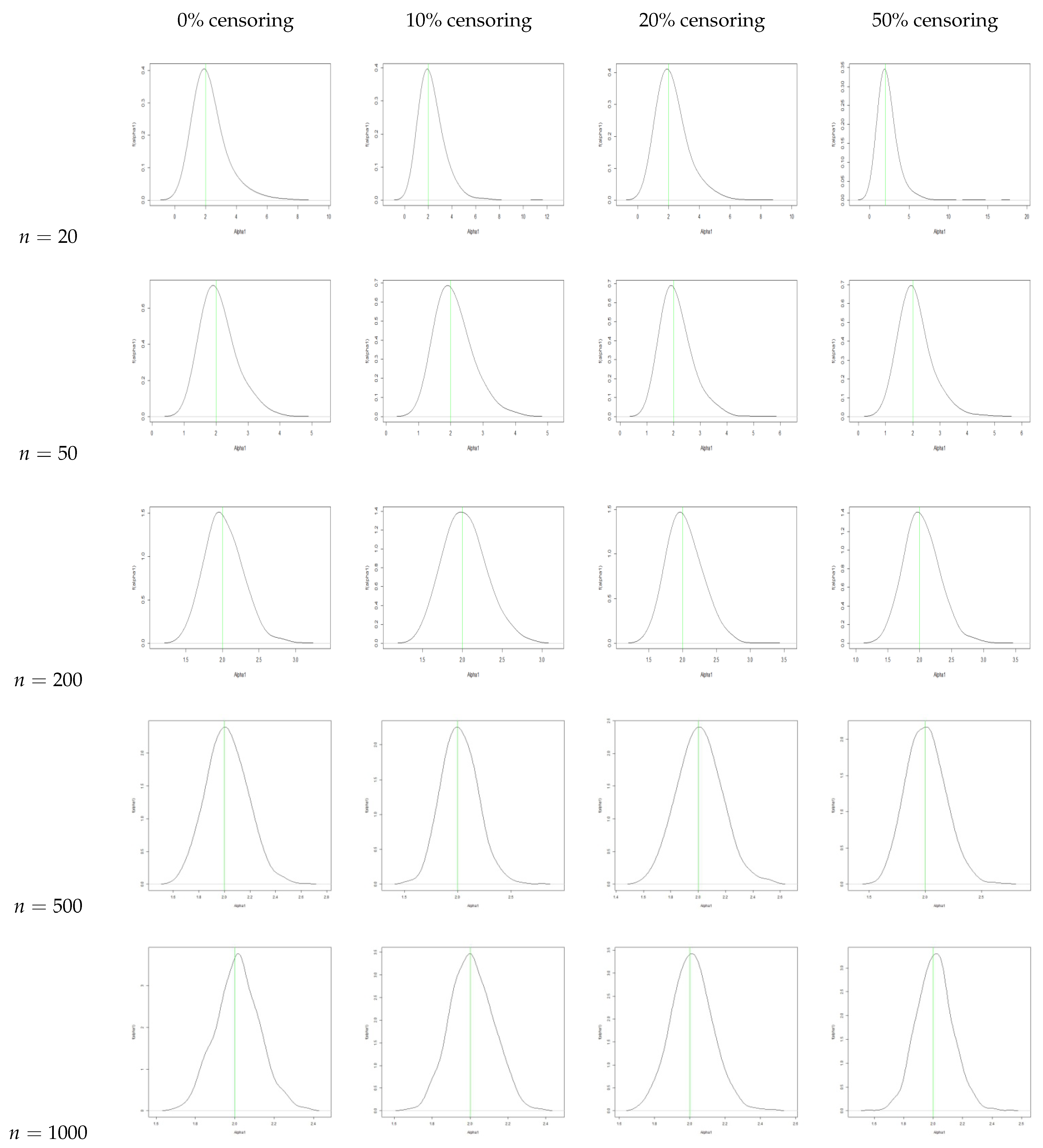
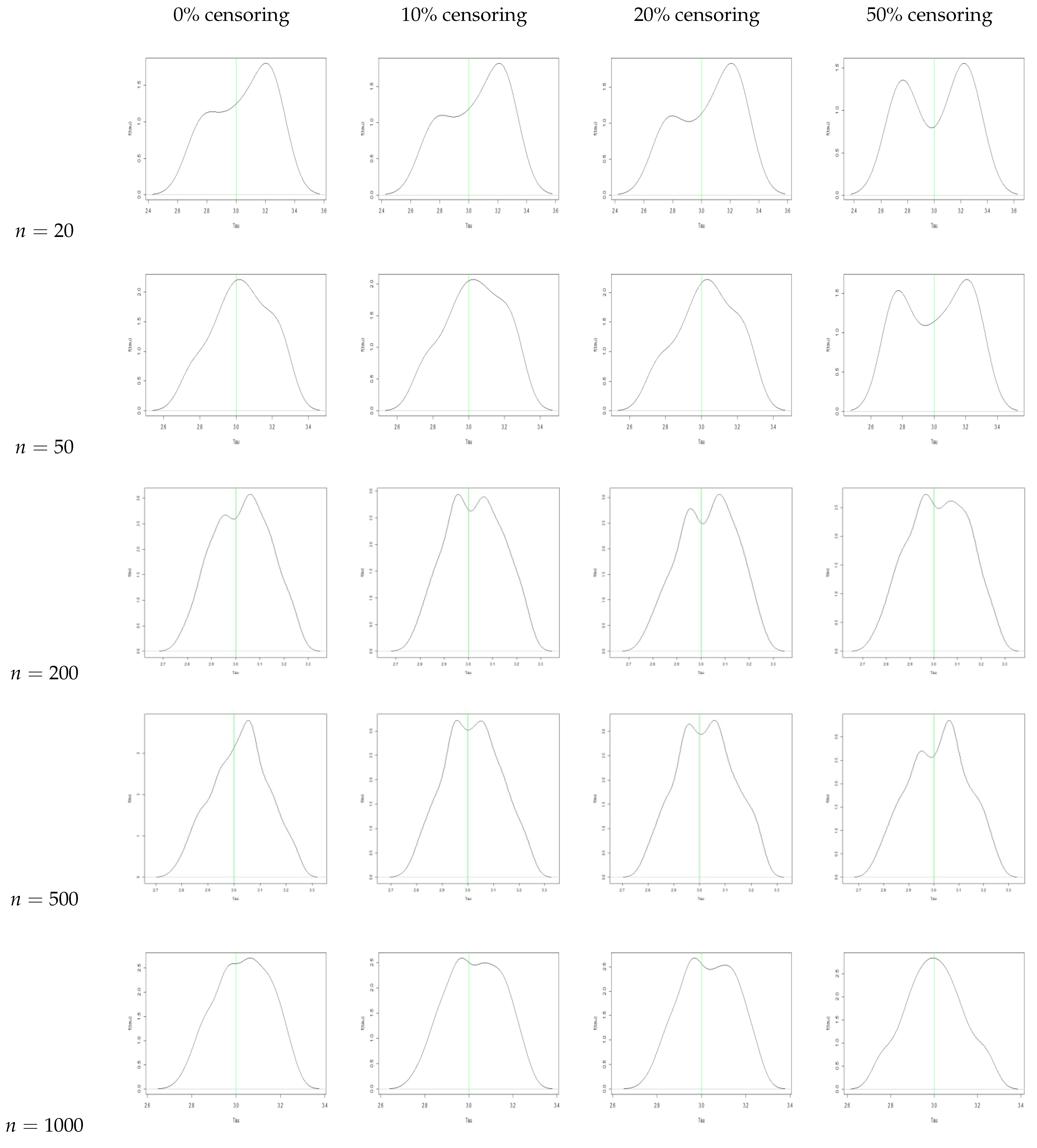
• We also plot the kernel density estimates to assess the normality. From Figure A4, Figure A5, Figure A6 and Figure A10, Figure A11, Figure A12, we see that the estimators are asymptotically normal. Here, in the case of 50% censoring when ${\alpha }_2=1$, we find that the kernel density estimator does not converge to normality at sample size 1000; however, the convergence can be achieved with a larger sample size.

5. Bayesian Analysis

We also establish the properties of the estimators obtained in Section 3 using a Bayesian analysis. We apply the Metropolis–Hastings (M-H) algorithm [23] and a Markov Chain Monte Carlo (MCMC) technique to estimate ${\alpha }_1,{\alpha }_2\mathrm{and}\tau$. We choose a normal distribution for all our three parameters (with an optimal choice of variance for all three parameters) as our proposal distribution.

If ${\tilde{\alpha }}_1,{\tilde{\alpha }}_2,\mathrm{and}\tilde{\tau }$ denote, respectively, the random variables ${\alpha }_1,{\alpha }_2,\mathrm{and}\tau$, they are then expressed as follows:

$${\tilde{\alpha }}_1\sim N({\alpha }_1,{0.5}^2),{\tilde{\alpha }}_2\sim N({\alpha }_2,{0.3}^2)\mathrm{and}\tilde{\tau }\sim N(\tau ,{0.7}^2)$$

Under a normal prior, the log of the posterior likelihood is given by the following:

$$\begin{array}{c}\hfill logL({\tilde{\alpha }}_1,{\tilde{\alpha }}_2,\tilde{\tau }|{\alpha }_1,{\alpha }_2,\tau ,\underline{x})\propto nlog{\tilde{\alpha }}_1-2\sum _{i=1}^n{ϵ}_{i}I(X_i\le \tilde{\tau })log(x_i+{\tilde{\alpha }}_1)-\sum _{i=1}^n(1-{ϵ}_i)I(X_i\le \tilde{\tau })log(x_i+{\tilde{\alpha }}_1)\\ \hspace{1em}\hspace{1em}-(n-u\left(\tilde{\tau }\right)-c\left(\tilde{\tau }\right))\left[log({\tilde{\alpha }}_1+\tilde{\tau })-log({\tilde{\alpha }}_2+\tilde{\tau })\right]-2\sum _{i=1}^n{ϵ}_{i}I(X_i>\tilde{\tau })log(x_i+{\tilde{\alpha }}_2)\hfill \\ \hspace{1em}\hspace{1em}-\sum _{i=1}^n(1-{ϵ}_i)I(X_i>\tilde{\tau })log(x_i+{\tilde{\alpha }}_2)-log\left(\sqrt{2\pi }0.5\right)-{\displaystyle \frac{1}{2}}{\left({\displaystyle \frac{{\tilde{\alpha }}_1-{\alpha }_1}{0.5}}\right)}^2-log\left(\sqrt{2\pi }0.3\right)\hfill \\ \hspace{1em}\hspace{1em}-{\displaystyle \frac{1}{2}}{\left({\displaystyle \frac{{\tilde{\alpha }}_2-{\alpha }_2}{0.3}}\right)}^2-log\left(\sqrt{2\pi }0.7\right)-{\displaystyle \frac{1}{2}}{\left({\displaystyle \frac{\tilde{\tau }-\tau }{0.7}}\right)}^2\hfill \end{array}$$

We run the algorithm 10,000 times. At each iteration i, a proposed value is generated from ${\underline{\theta }}^{\left(i\right)}\sim N({\underline{\theta }}^{(i-1)},{\sigma }^2)$, where ${\underline{\theta }}^{(i-1)}=({\tilde{\alpha }}_1^{(i-1)},{\tilde{\alpha }}_2^{(i-1)},{\tilde{\tau }}^{(i-1)})$ denotes the value of the parameters at the $(i-1)th$ iteration. The M-H algorithm is described as follows:

Algorithm:

• First, generate a proposal ${\theta }^{*}={\theta }^{\left(i\right)}$ from the proposal distribution $N({\underline{\theta }}^{(i-1)},{\sigma }^2)$.
• Next, compute the acceptance ratio, which is given as follows:

  $$r_i=min\left(1,{\displaystyle \frac{L\left({\theta }^{\left(i\right)}\right|{\alpha }_1,{\alpha }_2,\tau ,\underline{x})}{L\left({\underline{\theta }}^{(i-1)}\right|{\alpha }_1,{\alpha }_2,\tau ,\underline{x})}}\right)$$

  (4)
• Then, draw a random variable $u_i\sim U[0,1]$.
• If $u_i\le r_i$, accept the proposal and set ${\theta }^{*}={\theta }^{\left(i\right)}$; otherwise, reject the proposal and set ${\theta }^{*}={\theta }^{(i-1)}$.

We consider sample sizes of 20, 50, 200, 500, and 1000 under 0%, 10%, 20%, and 50%, censoring for the set of parameters ${\alpha }_1$ = 2, ${\alpha }_2$ = 1, and $\tau$ = 3. We do not discard the burn-in samples; we retain all 10,000 samples.

We plot trace plots for all parameters (shown in Figure A13, Figure A14, Figure A15) and tabulate the mean, bias, MSE, and the acceptance rate (AR), which is defined as the proportion of accepted samples out of the 10,000 simulated samples. The results are shown in

Table 3. Mean, bias, MSE and AR of the proposed log–logistic hazard change–point model based on 10,000 iterations of the Metropolis–Hastings algorithm for ${\alpha }_1$ = 2, ${\alpha }_2$ = 1, $\tau$ = 3.

		${\mathit{\alpha }}_1$			${\mathit{\alpha }}_2$			$\mathit{\tau }$			AR
Censoring	$\mathit{n}$	Mean	Bias	MSE	Mean	Bias	MSE	Mean	Bias	MSE
0%	20	1.9973	−0.0027	0.0640	0.9986	−0.0014	0.0081	2.9879	−0.0121	0.2465	0.9861
	50	1.9979	−0.0021	0.0637	1.0010	0.0010	0.0081	2.9895	−0.0105	0.2444	0.9906
	200	2.0017	0.0017	0.0622	1.0008	0.0008	0.0080	2.9929	−0.0071	0.2442	0.9948
	500	1.9994	−0.0006	0.0617	1.0006	0.0006	0.0080	2.9932	−0.0068	0.2430	0.9968
	1000	2.0005	0.0005	0.0612	0.9999	−0.0001	0.0079	2.9954	−0.0046	0.2427	0.9976
10%	20	1.9937	−0.0063	0.0643	0.9986	−0.0014	0.0082	2.9903	−0.0097	0.2426	0.9776
	50	1.9969	−0.0031	0.0642	0.9989	−0.0011	0.0082	2.9909	−0.0091	0.2406	0.9827
	200	2.0031	0.0031	0.0634	1.0003	0.0003	0.0081	2.9952	−0.0048	0.2391	0.9954
	500	1.9977	−0.0023	0.0627	1.0001	0.0001	0.0080	2.9959	−0.0041	0.2388	0.9961
	1000	1.9983	−0.0017	0.0625	0.9999	−0.0001	0.0080	2.9972	−0.0028	0.2370	0.9968
20%	20	1.9964	−0.0036	0.0631	0.9992	−0.0008	0.0082	2.9913	−0.0087	0.2451	0.9823
	50	1.9980	−0.0020	0.0628	0.9995	−0.0005	0.0081	2.9933	−0.0067	0.2408	0.9902
	200	1.998	−0.002	0.0626	1.0004	0.0004	0.008	2.9950	−0.0050	0.2404	0.9941
	500	1.9979	−0.0021	0.0622	1.0001	0.0001	0.0080	3.0038	0.0038	0.2361	0.9956
	1000	2.0001	0.0001	0.0621	1.0000	0.0000	0.0080	3.0017	0.0017	0.2347	0.9965
50%	20	1.9939	−0.0061	0.0624	0.9976	−0.0024	0.0083	2.9773	−0.0227	0.2421	0.9745
	50	1.9947	−0.0053	0.0630	0.9990	−0.0010	0.0082	2.9912	−0.0088	0.2413	0.983
	200	2.0005	0.0005	0.0630	1.0010	0.0010	0.0081	2.9919	−0.0081	0.2391	0.9949
	500	1.9979	−0.0021	0.0629	0.9999	−0.0001	0.0079	3.0049	0.0049	0.2386	0.9955
	1000	1.998	−0.002	0.0622	1.0000	0.0000	0.0078	2.9986	−0.0014	0.2361	0.9965

.

From Table 3 and from the trace plots, we observe the following:

• With an increase in sample size, there is a reduction in the bias and the MSE for all three parameters.
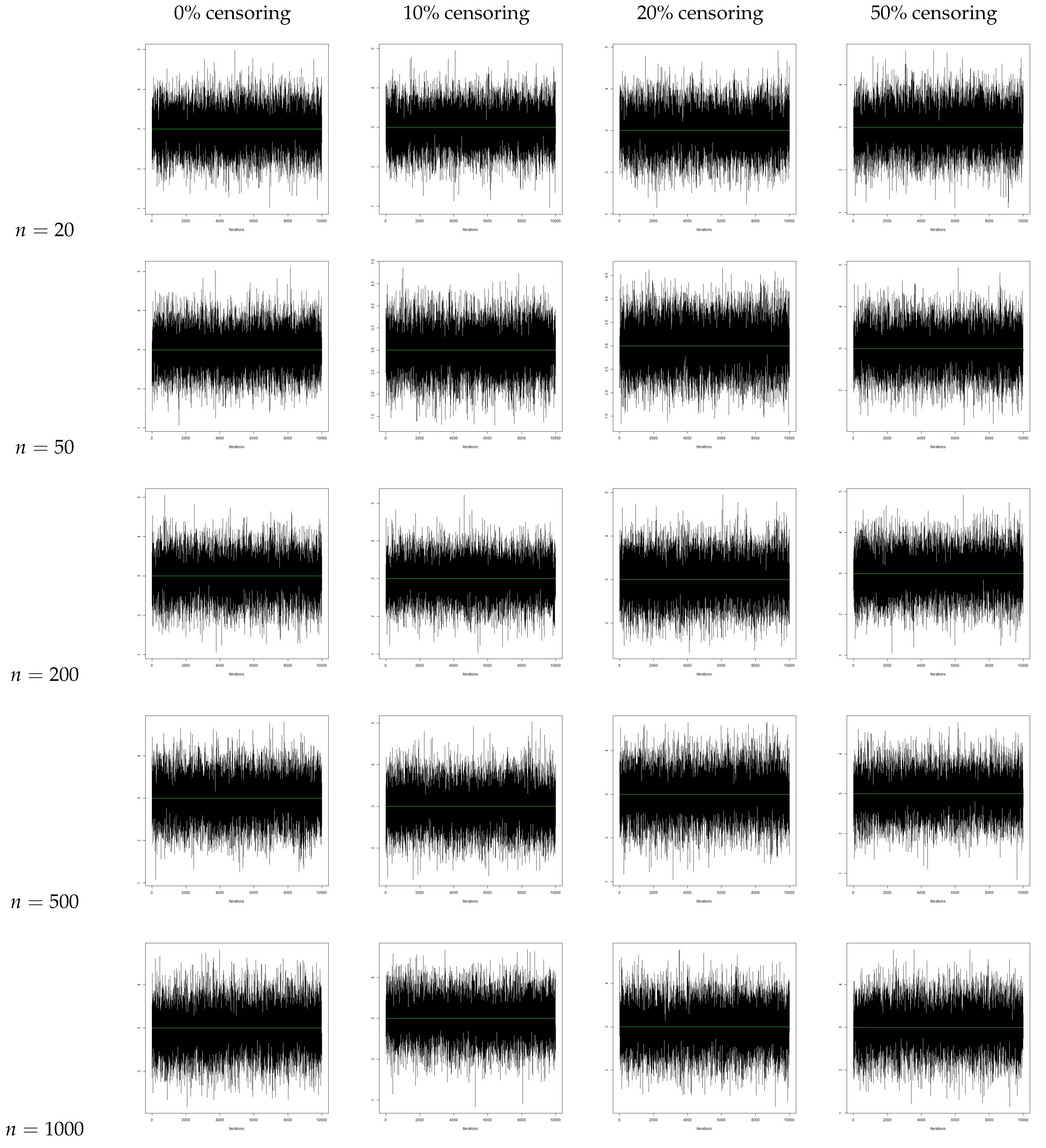
• We observe that the AR increases with an increase in sample size. We also see that the AR is lower for the same sample size when we increase the censoring percentage. Hence, we can infer that censoring has a slight effect on the AR of the samples.
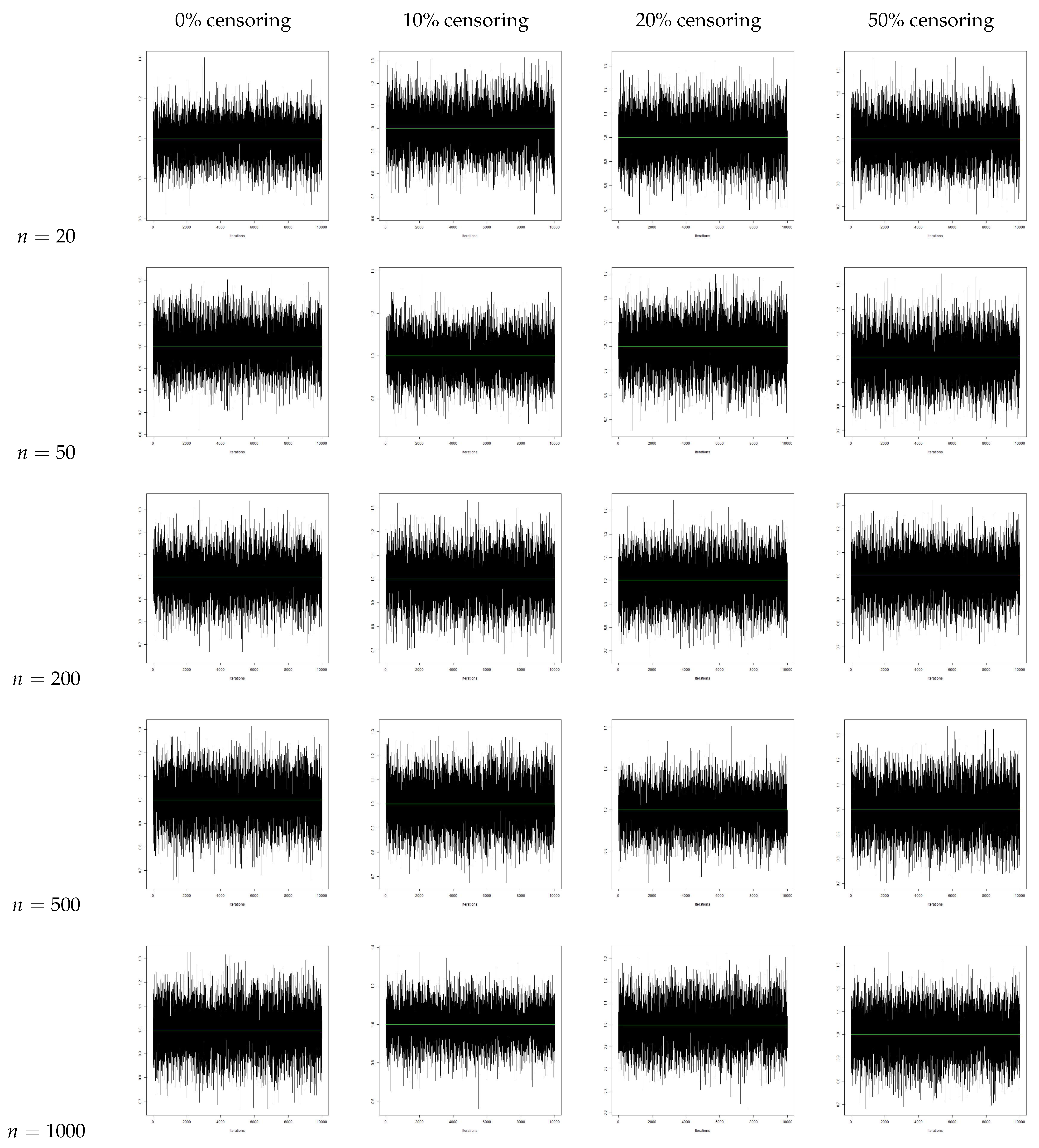
• From the traceplots, we see that there is no trend or fluctuation observed in any of the three parameters, indicating a good mix of the chain.

Comparing the Bayesian analysis with the PMLE, we find that the bias and MSE are significantly lower for the Bayesian analysis compared to the PMLE; this could be due to the greater number of iterations in the Bayesian scenario, as well as the use of normal priors with small variance as the proposal distribution. Overall, the simulation results and the Bayesian analysis indicate that the proposed estimators are asymptotically unbiased, consistent, and asymptotically normal.

6. Data Analysis

In this section, we apply the proposed log–logistic hazard change–point model (LLHM) to two real-life datasets and evaluate its performance by comparing it with the exponential hazard change–point model (EHM), the Lindley hazard change–point model [LHM], and the Weibull hazard change–point model [WHM].

• Model Evaluation Criteria and Goodness-of-Fit Measures

The AIC and BIC are defined as follows: [24]

AIC = −2 ln L + 2k, BIC = −2 ln L + k ln n

where ln L is the maximum value of the log-likelihood function for the estimated model, k is number of estimated parameters, and n is the sample size. Further, to assess the accuracy of the proposed model, the goodness-of-fit metrics—Manhattan distance ($L_1$ norm), Euclidean distance ($L_2$ norm), and Kolmogorov–Smirnov ($K\text{–}S$) statistic—are defined as follows:

$$\begin{array}{c}\hfill L_1\mathrm{norm},d_1(a,b)=\sum _{j=1}^n|a^{\left(j\right)}-b^{\left(j\right)}|\end{array}$$

$$\begin{array}{c}\hfill L_2\mathrm{norm},d_2(a,b)=\sqrt{\sum _{j=1}^n{(a^{\left(j\right)}-b^{\left(j\right)})}^2}\end{array}$$

$$\begin{array}{c}\hfill K\text{–}S\mathrm{statistic},d_3(a,b)=\underset{1\le k\le n}{max}\left|\sum _{j=1}^k{a}^{\left(j\right)}-\sum _{j=1}^k{b}^{\left(j\right)}\right|\end{array}$$

The Anderson–Darling (A-D) test is employed to determine whether the distribution of the model-generated data is statistically similar to that of the observed data. This test evaluates the null hypothesis $H_0$, which states that both samples are drawn from the same underlying distribution.

The A-D statistic is given by the following:

$$A^2=-n-{\displaystyle \frac{1}{n}}\sum _{i=1}^n(2i-1)\left[lnF\left(X_{\left(i\right)}\right)+ln\left(1-F\left(X_{(n+1-i)}\right)\right)\right]$$

where n is the sample size, $X_{\left(i\right)}$ are the ordered sample values, and F is the cumulative distribution function of the reference distribution (in this case, the empirical distribution of the observed data).

A high p-value (typically $p>0.05$) indicates that there is no statistically significant difference between the model and observed distributions, supporting the similarity assumption and indicating a good fit of the model to the data.

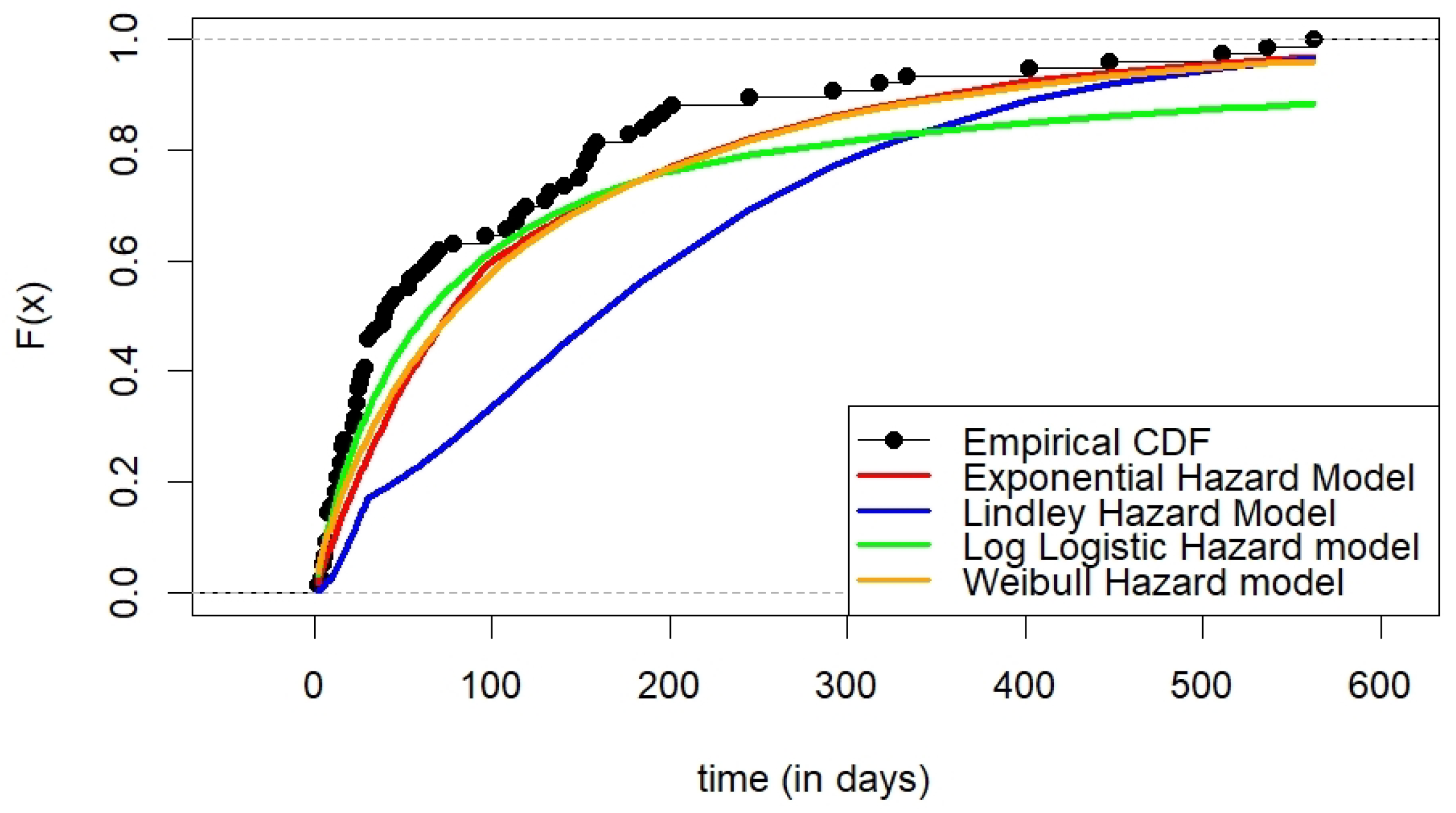
6.1. Kidney Catheter Data

The kidney dataset in the survival package is based on a medical study that investigated repeated kidney infection in patients following catheter treatment. A total of 76 patients were monitored over time to record the duration until a recurrence of infection, out of which 18 were censored. The dataset included information such as the time (in days) until the event of interest occurred, such as catheter failure or removal, censoring status, treatment type, and other related clinical details. The study was originally described in McGilchrist and Aisbett (1991).

Early catheter failures are frequently associated with acute complications, such as improper placement, immediate post-insertion infection, or suboptimal initial care. However, patients who avoid these early risks tend to reach a period of relative stability, during which the catheter can function effectively for an extended duration [25].

The change–point models are applied to the selected dataset. Model adequacy is assessed using the standard selection criteria, and their performance is evaluated through a range of predefined similarity and goodness-of-fit measures. The results of these evaluations are summarized in

Table 4. Parameter estimates of the change–point models when applied to data on recurrence times to infection of kidney patients.

Parameter	EHM	LHM	WHM	LLHM
${\alpha }_1$	0.0092	0.0239	62.2149	0.0170
${\alpha }_2$	0.0055	0.0088	143.7017	0.0155
$\tau$	96.0000	30.0000	107.9997	201.0000

and

Table 5. Different measures to assess the goodness of fit of the change–point models for Kidney Catheter data set.

Metrics	EHM	LHM	WHM	LLHM
AIC	684.5601	696.1884	681.1359	677.3659
BIC	691.5523	703.1806	688.1281	684.3581
$L_1$-norm	7.4771	16.4211	6.4272	5.1790
$L_2$-norm	1.0032	2.0890	0.8541	0.6724
$K\text{–}S$ statistic	0.2174	0.3620	0.1810	0.1351
$A\text{-}D$ test	2.605	11.07	1.891	1.658
$A\text{-}D$ asymptotic p-value	0.04279	0.0000	0.1041	0.1413

, with graphical representations of the cumulative distribution functions (CDFs) (Figure 2) illustrating how well each model fits the observed data.

From Table 5, it is observed that, among all the competing models, the proposed LLHM yields the smallest values across all distance-based evaluation metrics, indicating a better fit to the data. Also from the A-D test, the asymptotic p-value indicates that the proposed model is not significant at 5% level of significance and is therefore a good fit. Based on the analysis, from Table 4, a change–point is identified at 201 days and the scale parameter decreases from 0.0170 to 0.0155, i.e., there is an abrupt increase in the hazard rate after around 201 days, after which the infection increases at a faster rate, signaling catheter removal or failure. This finding also aligns with the fact that the median duration of catheter dialysis is 190 days [25].

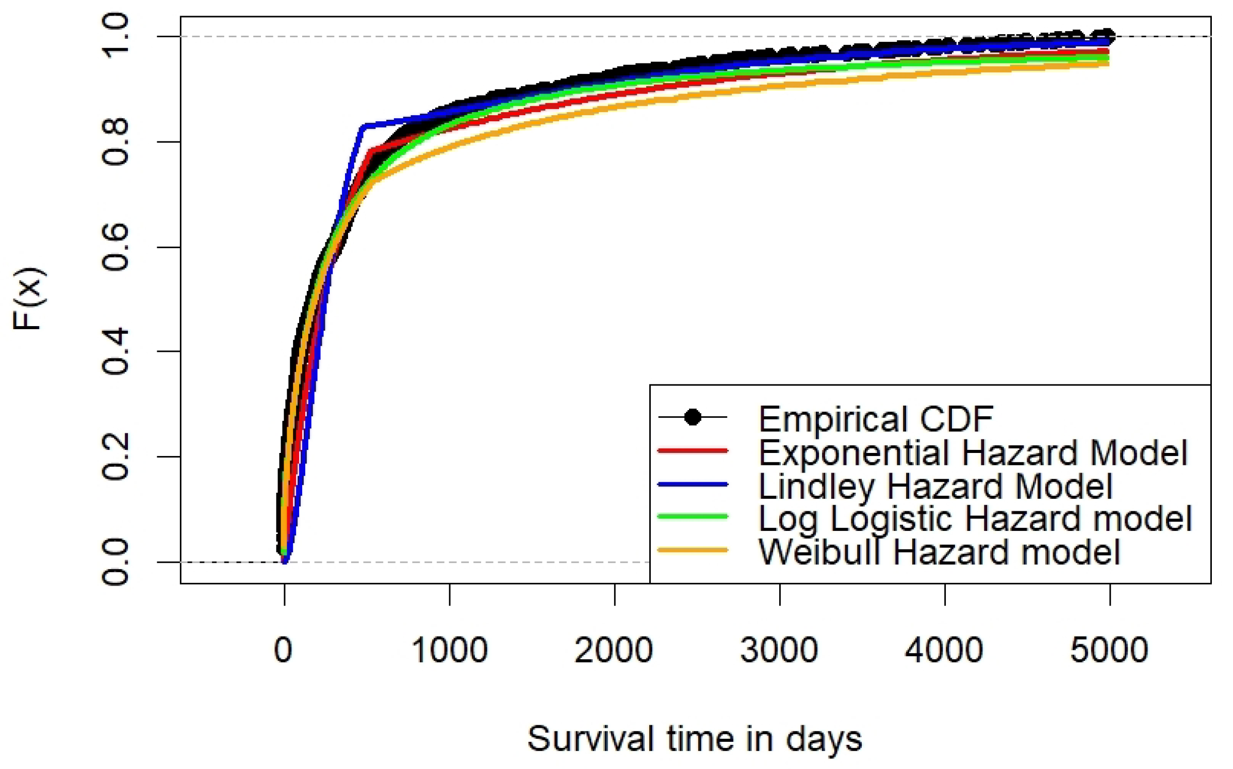
6.2. Acute Myeloid Leukemia

The analysis in this study is based on the LeukSurv dataset, which contains detailed survival data for 1043 patients diagnosed with acute myeloid leukemia (AML). It includes key variables such as time (in days) to event (death), event status (indicating death or censoring), age, sex, and white blood cell count (wbc) at diagnosis. For AML, the hazard rate plays a critical role in understanding disease progression and evaluating treatment outcomes. AML typically exhibits a high early hazard, especially during induction therapy, due to treatment-related toxicity and complications such as infections or bleeding [26].

The change–point models are applied to the selected dataset. Model adequacy is assessed using the standard selection criteria, and their performance is evaluated through a range of predefined similarity and goodness-of-fit measures. The results of these evaluations are summarized in

Table 6. Parameter estimates of change–point models when applied to data on duration of acute myeloid leukemia in patients.

Parameter	EHM	LHM	WHM	LLHM
${\alpha }_1$	0.0028	0.0066	0.01812	62.7735
${\alpha }_2$	0.0004	0.0008	0.0085	232.6557
$\tau$	527.0006	479.0017	534.9997	11.0000

and

Table 7. Different measures to assess the goodness of fit of the change–point models for Acute Myeloid Leukemia data set.

Metrics	EHM	LHM	WHM	LLHM
AIC	10,783.44	13,692.67	12,224.05	12,180.56
BIC	10,798.29	13,707.52	12,238.9	12,195.41
$L_1$-norm	71.4478	114.0331	22.5485	11.7279
$L_2$-norm	2.7499	4.4937	0.9709	0.4706
$K\text{–}S$ statistic	0.1531	0.2586	0.0671	0.0397
$A\text{-}D$ asymptotic p-value	0.0000	0.0000	0.0015	0.1225

, with graphical representations of the cumulative distribution functions (CDFs) (Figure 3) illustrating how well each model fits the observed data.

From the above-mentioned results (Table 6 and Table 7), the EHM shows lower $AIC$ and $BIC$ values, which might be due to the simplicity of the model as compared to LLHM. However, other evaluation measures such as the goodness-of-fit tests show higher values, indicating a poor fit of EHM to the data. This means that although EHM looks good based on $AIC$ and $BIC$, it does not capture the actual pattern of the data well. Apart from $AIC$ and $BIC$, the LLHM performs best across multiple evaluation criteria. It shows the smallest values in the $L_1$ norm, $L_2$ norm, and $K\text{–}S$ statistic, indicating that its CDF curve is closest to the observed data. Additionally, the $A\text{-}D$ test yields a p-value that is not significant at 5% level of significance, further supporting that the model fits the data well.

The WHM, LLHM, and EHM estimate delayed change-points ranging from approximately 479 to 535 days. Among these, the LLHM identifies a change–point at 11 days, indicating a sharp increase in hazard very early in the disease course. From Table 6, a small change–point indicates that the risk of failure (e.g., death or relapse) is initially high during the early weeks after diagnosis. However, the increase in the scale parameter after this early change–point suggests that patients who survive this critical early period tend to have a slower progression of risk over time. This finding of a change–point at 11 days is consistent with the fact that the maximum risk of death due to AML occurs within 3–4 weeks after start of the treatment [26].

7. Conclusions and Future Work

In this paper, we introduce a log–logistic hazard model in the presence of a change–point. We derive expressions for the PDF and the survival function. We then estimate parameters using the PMLE and study the estimators obtained using different statistical measures and plots. The proposed change–point model is applied to both the Kidney Catheter and the Acute Myeloid Leukemia datasets and compared with the EHM, LLHM, and WHM. In both cases, LLHM provides the best fit, as indicated by lower values in the distance-based metrics (e.g., $K\text{–}S$ statistic, $L_1$ and $L_2$ norms) and the A-D test asymptotic p-value.

Interestingly, the change–point occurred earlier in the AML dataset, and the scale parameter increased after the change–point, suggesting that risk was highest in the early phase, but patients who survived this period tended to have slower hazard progression. In contrast, the Kidney Catheter dataset showed a later change–point with a decrease in the scale parameter, indicating that the patients were initially relatively stable, but hazard increased more sharply beyond a certain time, aligning with the possibility of delayed complications such as infections. These findings demonstrate the flexibility and clinical relevance of the LLHM in capturing disease-specific survival dynamics.

We may further extend the log–logistic change–point model to test for the presence of multiple change-points in a dataset, as well as the presence of covariates, so as to enhance the applicability of this model to diverse fields.

References

1. Gupta, R.C.; Olcay, A.; Sergey, L. A study of log-logistic model in survival analysis. Biom. J. J. Math. Methods Biosci. 1999, 41, 431–443. [Google Scholar] [CrossRef]
2. Steve, B. log–logistic regression models for survival data. J. R. Stat. Soc. Ser. C Appl. Stat. 1983, 32, 165–171. [Google Scholar]
3. Muse, A.H.; Mwalili, S.; Oscar, N. On the log–logistic distribution and its generalizations: A survey. Int. J. Stat. Probab. 2021, 10, 93. [Google Scholar] [CrossRef]
4. Lemonte, A.J. The beta log–logistic distribution. Braz. J. Probab. Stat. 2014, 28, 313–332. [Google Scholar] [CrossRef]
5. Fahim, A.; Mahdi, S. Fitting the log–logistic distribution by generalized moments. J. Hydrol. 2006, 328, 694–703. [Google Scholar]
6. Shoukri, M.M.; Mian, I.U.H.; Tracy, D.S. Sampling properties of estimators of the log-logistic distribution with application to Canadian precipitation data. Can. J. Stat. 1988, 16, 223–236. [Google Scholar] [CrossRef]
7. De Santana, T.V.F.; Ortega, E.M.; Cordeiro, G.M.; Silva, G.O. The Kumaraswamy-log–logistic distribution. J. Stat. Theory Appl. 2012, 11, 265–291. [Google Scholar]
8. Ramos, P.L.; Balakrishnan, N.; Zografos, K. The Zografos-Balakrishnan log–logistic distribution: Properties and applications. J. Stat. Theory Appl. 2013, 12, 275–290. [Google Scholar]
9. Alfaer, N.M.; Gemeay, A.M.; Aljohani, H.M.; Afify, A.Z. The extended log–logistic distribution: Inference and actuarial applications. Mathematics 2021, 9, 1386. [Google Scholar] [CrossRef]
10. Felipe, A.; Jaenada, M.; Miranda, P.; Pardo, L. Robust parameter estimation of the log–logistic distribution based on density power divergence estimators. arXiv 2023, arXiv:2312.02662. [Google Scholar] [CrossRef]
11. Gaire, A.K.; Gurung, Y.B. Rayleigh generated log–logistic distribution properties and performance analysis. J. Turk. Stat. Assoc. 2024, 15, 13–28. [Google Scholar]
12. Matthews, D.E.; Farewell, V.T. On Testing for a Constant Hazard against a Change-Point Alternative. Biometrics 1982, 38, 463–468. [Google Scholar] [CrossRef]
13. Chang, I.S.; Chen, C.H.; Hsiung, C.A. Estimation in Change-Point Hazard Rate Models with Random Censorship. Lect. Notes-Monogr. Ser. 1994, 23, 78–92. [Google Scholar]
14. Gijbels, I.; Gürle, U. Estimation of a Change-Point in a Hazard Function Based on Censored Data. Lifetime Data Anal. 2003, 9, 395–411. [Google Scholar] [CrossRef] [PubMed]
15. Goodman, M.S.; Li, Y.; Tiwari, R.C. Detecting Multiple Change-Points in piece-wise Constant Hazard Functions. J. Appl. Stat. 2011, 38, 2523–2532. [Google Scholar] [CrossRef]
16. Williams, M.R.; Kim, D.Y. A test for an Abrupt Change in Weibull Hazard Functions with Staggered Entry and Type-I Censoring. Commun. Stat. Theory Methods 2013, 42, 1922–1933. [Google Scholar] [CrossRef]
17. Joshi, S.; Jose, K.K.; Bhati, D. Estimation of a Change-Point in the Hazard Rate of Lindley Model under Right Censoring. Commun. Stat. Simul. Comput. 2017, 46, 3563–3574. [Google Scholar] [CrossRef]
18. Palmeros, O.; Villaseñor, J.A.; González, E. On computing estimates of a change–point in the Weibull regression hazard model. J. Appl. Stat. 2018, 45, 642–648. [Google Scholar] [CrossRef]
19. Joshi, S.; Rattihalli, R.N. Estimation of parameters in a general hazard regression change–point model. J. Indian Stat. Assoc. 2019, 57, 19–40. [Google Scholar]
20. Joshi, S.; Rattihalli, R.N. Estimation of Parameters in the Exponential-Lindley Hazard Change-Point Model. Adv. Intell. Syst. Comput. 2020, 1169, 345–356. [Google Scholar]
21. Gierz, K.; Park, K. Detection of multiple change points in a Weibull accelerated failure time model using sequential testing. Biom. J. 2022, 64, 617–634. [Google Scholar] [CrossRef] [PubMed]
22. Matloff, N. The Art of R Programming: A Tour of Statistical Software Design; No Starch Press: San Francisco, CA, USA, 2011. [Google Scholar]
23. Lynch, S.M. Introduction to Applied Bayesian Statistics and Estimation for Social Scientists; Springer: New York, NY, USA, 2007; Volume 1. [Google Scholar]
24. Akaike, H. A new look at the statistical model identification. IEEE Trans. Automat. Contr. 1974, 19, 716–723. [Google Scholar] [CrossRef]
25. Griffith, I.R.; Newsome, B.B.; Leung, G.; Block, G.A.; Herbert, R.J.; Danese, M.D. Impact of Hemodialysis Catheter Dysfunction on Dialysis and Other Medical Services: An Observational Cohort Study. Int. J. Nephrol. 2012, 8, 1179–1187. [Google Scholar] [CrossRef]
26. Walter, R.B.; Othus, M.; Borthakur, G.; Ravandi, F.; Cortes, J.E.; Pierce, S.A.; Appelbaum, F.R.; Kantarjian, H.A.; Estey, E.H. Prediction of early death after induction therapy for newly diagnosed acute myeloid leukemia with pretreatment risk scores: A novel paradigm for treatment assignment. J. Clin. Oncol. 2011, 29, 4417–4423. [Google Scholar] [CrossRef] [PubMed]
Figure 1. Hazard function of the log–logistic distribution at the change–point.
Mathematics 13 01457 g001
Figure 2. CDF Curves of kidney catheter data set under different models.
Mathematics 13 01457 g002
Figure 3. CDF Curves of acute myeloid leukemia data set under different models.
Mathematics 13 01457 g003