Abstract
This article first selects the “Urban Statistical Yearbook” data of 264 prefecture-level cities in China from 2004 to 2018 as the raw data, and uses principal component analysis and the Wilson model to calculate the spatial information diffusion capacity of each prefecture-level city. The correlation analysis between industrial agglomeration, spatial information diffusion capacity, and urban economic resilience is verified, and this article provides reference materials for the specific application of principal component analysis and the Wilson model in urban economics.
Keywords:
principal component analysis; Wilson model; spatial information diffusion capability; urban economics MSC:
37M99
1. Introduction to the Concept of Spatial Information Diffusion and the Theoretical Framework of Urban Spatial Information Diffusion
Spatial information diffusion refers to the process of information spreading to the outside world through various media in a transactional or non-transactional manner, which comes from the circulation and diffusion of information. Its advantages for social development are increasing the speed of information flow and promoting social progress. But the negative impact it brings to society cannot be ignored. Firstly, the diffusion of spatial information leaks personal privacy and information security, which can bring unfair competition to the market. For example, some information reflects the sensitive information of citizens, and the leakage of personal privacy can easily cause the leakage of individual, organizational, and commercial secrets. With the development of society, the weight of information in the economic operation of society continues to strengthen, and the spatial distribution of industries has created the birth of information radiation centers (information radiation centers refer to centers in a region or institution that have a wide impact and radiation effect on surrounding regions or countries through information dissemination and technological exchange). At the same time, due to the information asymmetry between manufacturers and markets, this exacerbates the dependence of industry development on information hinterlands (information hinterlands are usually resource-rich areas that can provide energy, minerals, agricultural products, etc., needed for economic development, supporting the industrial development of the region). Therefore, spatial information diffusion, as an intermediate bridge of industrial clusters, can promote a positive interactive mechanism bridge between industrial clusters and the resilient development of urban economy. Enterprises can expand their market share at home and abroad and increase market interest in investors by publicly disclosing demand information. And enterprises can also grasp real-time market news at home and abroad through publicly available information, which can identify market demand dynamics and avoid unnecessary risks and troubles. The spatial information diffusion effect is similar to a magnet, exerting a centripetal force on the distribution of industrial clusters.
Hypothesis 1:
The diffusion effect of spatial information has a positive promoting effect on the development of diversified industrial agglomeration. The new economic growth theory holds that the positive externality of spatial information diffusion effect is the intrinsic driving force for promoting industrial agglomeration development. The spatial information diffusion effect and industrial agglomeration are linked through the proximity of geographical locations between industries and between enterprises. Baldwin and Forslid (1999) argue that industrial agglomeration and spatial information spillover effects can promote urban economic growth, which is independent of the velocity of capital flow. This indicates that spatial spillover effects have a positive promoting effect on the development of industrial agglomeration [1]. Ottaviano and Martin (2001) hypothesized that production factors within industrial agglomeration areas are immobile, established a self-reinforcing model of economic growth and spatial agglomeration, and concluded that industrial agglomeration can promote knowledge dissemination and technology overflow within the agglomeration area through spatial information diffusion effects, thereby reducing the cost and risk of enterprise innovation [2]. Fujita (1999) believe that the development of industrial clusters can not only enhance local market competitiveness, but also drive the development of surrounding industries through spatial information diffusion effects, and attract more talents and resources to serve the local area, thereby further enhancing the agglomeration advantage of local industries. Although the research hypotheses and backgrounds of various scholars are different, the conclusions obtained are basically consistent, that is, the spatial information diffusion effect shows a positive correlation with industrial agglomeration. Based on the existing literature, this article further proves the authenticity of Hypothesis 1 through empirical analysis [3].
Hypothesis 2:
There is a significant mutual influence effect between spatial information diffusion and urban economic resilience. The impact mechanism of spatial information diffusion on urban economic resilience can be analyzed from the perspectives of supply and demand. From the perspective of demand, feedback from the market to the supply side can help related industries quickly understand market demand, organize and operate production in a timely manner, and incorporate new ideas into the production process, thereby optimizing product quality and improving industry resilience. From the perspective of supply, the positive externalities of spatial information diffusion on urban economic resilience originated from Marshall’s theory of externalities. Marshall (1920) believed that only when companies in the same or related industries gather together can specialized labor aggregation, intermediate product input in related fields, and the generation of knowledge and technology sharing be promoted. The enhancement of industrial innovation capability is the fundamental way to promote urban economic resilience, but the fundamental methods of promoting industrial innovation are the sharing of knowledge within or between industries, the introduction of talents, and the spillover effects of technology. Knowledge can be divided into explicit and implicit knowledge. Explicit knowledge can be improved through learning from textbooks and media. Implicit knowledge can only be acquired through information exchange and spatial information diffusion. Only by being geographically adjacent to industrial clusters and being close to the information hinterland can advanced production technologies and business knowledge be imitated and improved. Due to the accumulation of a large amount of knowledge, technology, and human capital within industrial clusters, it is easy to achieve positive externalities on the surrounding areas through spatial information diffusion effects, which not only helps the development of the surrounding areas but also attracts more high-quality resources to the local area, thereby promoting the joint development of local and surrounding cities’ economic resilience [4].
2. Introduction to the Theory of Wilson Model
The measurement of urban spatial information diffusion capability can be traced back to the Wilson model. According to Liang Lin (2014) [5], measuring the spatial information diffusion capability of each city first requires calculating the information radiation radius of each city. However, Wilson provided ideas and methods for measuring urban information radiation capability. Wilson was a famous physicist in the 1970s. There is a mutual interaction relationship between two neighboring cities or cities with close communication, which is related to the distance between the two cities. The Wilson model is currently widely used in information radiation in various industries. This article will measure the spatial information diffusion capacity of 264 prefecture-level cities in China. The premise of applying the Wilson model is that all macro- and micro-level events have the same probability. The formation of a region is mainly composed of different node regions. According to the law of conservation of energy, the energy input of one region to another region is equivalent to the energy output of another region in that region. Referring to Liang Lin (2014) [5], the formula expression for the gate valve value θ of the spatial information diffusion ability of a certain city i to another city j is shown in Formula (1):
θ = Tiexp(−βɣij)
T represents the maximum output of resources from one region to another, or the input of resources from another region to a certain region. The logarithm of both sides of the equation is taken simultaneously to obtain the spatial information diffusion radius r, which is the spatial information diffusion effect model shown in Formula (2):
r = (1/β) × ln(Ti/θ)
By performing extreme evaluation on (2), the following three relationships can be obtained, as shown in Equations (3)–(5):
if β → +∞, ɣ = lim(1/β) × ln(Ti/θ) = 0
if β → 0, ɣ = lim(1/β) × ln(Ti/θ) = +∞
if β → 1, ɣ = lim(1/β) × ln(Ti/θ) = ln(Ti/θ)
In the process of setting indicators for spatial information diffusion, refer to Table 1:

Table 1.
Indicator setting of spatial information diffusion capability in various cities.
In Table 1, these three criteria can be subdivided into 10 different indicators, and we can use factor analysis to measure the total amount of spatial information diffusion in China. Currently, many cities in eastern China have become growth centers for spatial information diffusion. With the adjustment of economic structure, the economic situation of central and western cities is gradually stabilizing and rising. So what is the spatial information diffusion capability of each city, and what is the correlation between industrial agglomeration, spatial information diffusion, and urban economic resilience? These are the issues we will discuss next. Referring to Liang Lin (2014) [5], in order to solve the problem of inconsistent units among the selected indicators and avoid deviation caused by large variances in the calculated results, the collected data were standardized and factor analysis was used to reduce the dimensionality of the selected indicators using SPSS 29.0 software. Before conducting factor analysis, it is necessary to use KMO (Bartlett sphericity test) to test the correlation and collinearity between the selected indicators, in order to determine whether factor analysis can be used, as shown in Table 2:
Table 2.
Bartlett’s test of sphericity KMO test results (2004–2018).
From a statistical perspective, a KMO value exceeding 0.6 is suitable for factor analysis, and the larger the KMO value, the higher the collinearity of the model, making it more suitable for using factor analysis to process data. According to the results in Table 2, the value of KMO is 0.807, which is larger than 0.6; the significant term 0.000 is smaller than 0.01, thus rejecting the assumption that the matrix is an identity matrix. This indicates that the variables in the model have collinearity and are suitable for dimensionality reduction. Factor analysis was used to process the data. The main idea of factor analysis is dimensionality reduction. As shown in Table 3, we can select two common factors to replace the original 12 indicators to measure the spatial information diffusion ability of cities. The cumulative variance contribution rate of these two common factors is 59.397%.
Table 3.
Analysis of variance contribution (2004–2018).
We can use a variance contribution analysis chart and apply the principle of variance maximization to rotate each factor to illustrate the proportion of the two common factors we have selected in order to simplify the model and explain the factors, as shown in Figure 1 and Table 4 and Table 5.
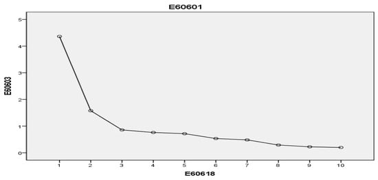
Figure 1.
Analysis of variance contribution (2004–2018).
Table 4.
Factor loading results after orthogonal rotation (2004–2018).
Table 5.
Principal factor load analysis table (2004–2018).
We analyzed the proportions of the ten selected indicators in the two principal components, and the specific proportions are shown in Table 6, resulting in Models (6)–(8):
T1 = 0.152X1 − 0.094X2 − 0.092X3 + 0.260X4 + 0.218X5 + 0.105X6 + 0.259X7 + 0.108X8 + 0.156X9 + 0.081X10
T2 = 0.114X1 + 0.358X2 + 0.443X3 − 0.218X4 − 0.095X5 + 0.245X6 − 0.246X7 + 0.117X8 + 0.07X9 + 0.232X10
T = 0.4364T1 + 0.1576T2
Table 6.
Score coefficient matrix for each component (2004–2018).
According to Formula (8), combined with Table 1 and standardized processing, we can calculate the comprehensive score T of the total information resources of 264 prefecture-level cities in China from 2004 to 2018. The larger the T value, the greater the total information resources of the city, and the smaller the T value, the smaller the spatial information diffusion resources of the city. Because according to principal component analysis, cities with a comprehensive score of less than 5 in total information resources have a comprehensive score of less than one-thousandth in principal component analysis, their effect can be ignored. Therefore, we set the threshold value to 5, which means that the city does not have the qualification for information spillover if it is less than 5.
In the process of measuring 264 prefecture-level cities in China, a total of 114 prefecture-level cities had information scores exceeding 5 from 2004 to 2018, making them radiation cities for spatial information diffusion. There are 58 cities in the eastern region, including 11 cities in Guangdong Province, 8 cities in Zhejiang Province, 11 cities in Shandong Province, 2 cities in Liaoning Province, 13 cities in Jiangsu Province, 3 cities in Hebei Province, 1 city in Hainan Province, and 6 cities in Fujian Province, in addition to Beijing, Shanghai, and Tianjin. There are 32 cities in central China, including 2 cities in Shanxi Province, 4 cities in Jiangxi Province, 6 cities in Hunan Province, 8 cities in Hubei Province, 11 cities in Henan Province, and 1 city in Anhui Province. There are 19 cities in the western region, including 2 cities in Yunnan Province, 1 city in Xinjiang, 5 cities in Sichuan Province, 4 cities in Shaanxi Province, 1 city each in Qinghai, Ningxia, Inner Mongolia, Guangxi, and Gansu, and 2 cities in Guizhou. Table 7 lists the top 20 cities in terms of spatial information diffusion resource capability.
Table 7.
Top 20 cities in terms of comprehensive score of total information resources among 264 prefecture-level cities in China (2004–2018).
Next, we selected the Wilson model (Model (9)) to measure the information radiation radius of 264 prefecture-level cities in China from 2004 to 2018. The Chinese scholars Liang Lin (2014) [5] also used the Wilson model in their research on population mobility and information radiation, and summarized the measurement formula for information attenuation factor as follows:
In Formula (9), T represents the total sample size of the research city. We selected 264 prefecture-level cities in China, so T = 264; Tmax represents the cities in the sample that have information radiation capabilities. Based on the data analysis in the previous section, we found that there were 114 cities with information radiation capabilities from 2004 to 2018. Therefore, tmax = 114. D represents the average administrative area of the 264 prefecture-level cities in China that we selected. According to the urban statistical yearbook, we calculated D = 16,111.1 km2. Using Formula (9), we can obtain the information radiation attenuation factor of 0.0170 for the 264 prefecture-level cities we selected from 2004 to 2018. Therefore, based on Formula (2), we can obtain the information radiation radius of the 264 prefecture-level cities in China from 2004 to 2018. The information radiation radius of a city is the spatial information diffusion effect of the city.
3. Measurement of Spatial Information Diffusion in Chinese Prefecture-Level Cities
We usually use (ifo) to represent the spatial information diffusion effect. Currently, there are many methods used to measure the spatial information diffusion mode of enterprises. In this article, we mainly use certain indicators that can reflect the spatial information diffusion degree of enterprises as alternative indicators. As shown in Table 1, these three criteria can be subdivided into 10 different indicators. We refer to Liang Lin’s (2014) [5] selection of the Wilson model to measure the spatial information diffusion capacity of 264 prefecture-level cities in China, as shown in Model (10):
ifo = (1/β) × ln(Ti/θ)
In Model (10), β represents the attenuation factor of urban spatial information diffusion effect, ifo is the spatial information diffusion effect of the city, and θ is a threshold set for the spatial information diffusion effect of the selected 264 prefecture-level cities in this paper. When the spatial information diffusion effect of a city is lower than a certain threshold, we assume that the city is the recipient of the spatial information diffusion effect. When the spatial information diffusion effect of this city exceeds a certain threshold, we set the threshold in this article to 5. When T > 5, we can consider this city to have spatial information diffusion effect.
This article mainly uses data from 264 prefecture-level cities in China from 2004 to 2018, sourced from the China Urban Statistical Yearbook. Firstly, when measuring the spatial information diffusion capability of a city, as shown in Table 1, we included three aspects: information infrastructure, information development scale, and information subjects. The spatial information diffusion ability of the 264 prefecture-level cities selected in this article shows that 114 cities have spatial information diffusion effects exceeding the threshold, therefore tmax = 114. This indicates that from 2004 to 2018, 114 cities out of these 264 prefecture-level cities have the output ability of spatial information diffusion. Among these 114 cities, the eastern cities account for 50.8%, the central cities account for 33.3%, and the western cities account for 15.9%. According to the data on administrative land area in the 2004–2018 China City Statistical Yearbook, D = 16,111.1 km2 was calculated. Therefore, the attenuation factor β of spatial information diffusion effect in 264 prefecture-level cities in China from 2004 to 2018 is 0.0169. Based on these data, the spatial information diffusion radius and spatial information diffusion effect data score of 264 prefecture-level cities in China from 2004 to 2018 can be calculated, as shown in Table 8.
Table 8.
Top 20 cities with information effect scores among 264 prefecture-level cities in China (2004–2018).
Next, we selected the Wilson model (Model (11)) to measure the information radiation radius of 264 prefecture-level cities in China from 2004 to 2018. The Chinese scholars Lin (2014) [5] also used the Wilson model in their research on population mobility and information radiation, and summarized the measurement formula for information attenuation factor:
In Formula (11), T represents the total sample size of the research city. We selected 264 prefecture-level cities in China, so T = 264; Tmax represents the cities in the sample that have information radiation capabilities. Based on the data analysis in the previous section, we found that there were 114 cities with information radiation capabilities from 2004 to 2018. Therefore, tmax = 114. D represents the average administrative area of the 264 prefecture-level cities in China that we selected. According to the urban statistical yearbook, we calculated D = 16,111.1 km2. Using Formula (11), we can obtain the information radiation attenuation factor of 0.0170 for the 264 prefecture-level cities we selected from 2004 to 2018. Therefore, based on Formula (8), we can obtain the information radiation radius of the 264 prefecture-level cities in China from 2004 to 2018. The information radiation radius of a city is the spatial information diffusion effect of the city.
4. Empirical Results and Analysis
4.1. Descriptive Statistical Analysis
The spatial information diffusion resource capacity of 264 prefecture-level cities in China has been measured and described above. In order to further analyze the relationship between industrial agglomeration, spatial information diffusion, and urban economic resilience, this paper uses urban panel data from 2004 to 2018 to test the correlation between industrial agglomeration, spatial information diffusion, and urban economic resilience. The descriptive statistics of each variable are shown in Table 9.
Table 9.
Descriptive statistics of variables (2004–2018).
Through the descriptive statistics of variables in Table 9, we can see that the dependent variable, urban economic resilience, and the standard deviation of the explanatory variable are both very large. This indicates that there are significant differences in economic resilience, industrial agglomeration level, and spatial information diffusion ability among cities in different geographical locations in China. This also indicates that China has a vast geographical area, and there is still a lot of room for improvement in the economic resilience and development status of underdeveloped cities. We took resilience of urban economy as the explained variable; resilience t − 1, the industrial agglomeration item nonagr, and the spatial information diffusion item ifo as the main explained variables; and the proportion of the primary industry in GDP, the proportion of the tertiary industry in GDP, FDI in GDP, and fixed assets investment in GDP as the control variables. We divided the 264 prefecture-level cities in China we selected into three categories: eastern, central, and western. The expression is as shown in Formula (11):
resiliencez,t = aresiliencez,t−1 + βnonoagrz,t + cifoz,t + rXz,t +uz + §z,t
4.2. Benchmark Regression Analysis
According to statistical description, the so-called individual fixed effect refers to the impact on the stability of the model we set up when the sample we study changes with spatial variation but not with temporal variation. The time fixed effect refers to the impact on the stability of the model we set up when it changes with time and does not change with space. We performed the Lagrange test, Robust test, and correlation test between fixed effects and time effects on Formula (9) to choose which test method is more suitable in Formula (9).
Table 10 provides estimates and tests for the correlation between industrial agglomeration, spatial information diffusion, and urban economic resilience using a non-spatial-panel, non-fixed-effects model. Table 10 reports the OLS benchmark regression results of this chapter. From a national perspective, the impact of industrial agglomeration on urban economic resilience is significantly positive at the 1% level. For every 1 percentage point increase in industrial agglomeration, urban economic resilience will increase by 1585.307 percentage points. The impact of spatial information diffusion on urban economic resilience is significantly positive at the 5% level, and for every 1 percentage point increase in spatial information diffusion, urban economic resilience will increase by 0.0732 percentage points. In columns (2), (3), and (4), eastern, central, and western cities were added, respectively. It was found that the impact of industrial agglomeration on urban economic resilience was significantly positive at the 1% level in eastern, central, and western cities. Moreover, for every 1 percentage point increase in industrial agglomeration, urban economic resilience increased by 1000.05, 6881.75, and 46,678.79 percentage points in eastern, central, and western cities, respectively. The spatial information diffusion resources are significantly positive at the 5% level in both eastern and central cities, and for every 1 percentage point increase in the spatial information diffusion term, the urban economic resilience level increases by 0.012 and 0.0369 percentage points, respectively. The impact of spatial information diffusion on urban economic resilience in western cities is significantly negative at the 5% level, and for every 1 percentage point increase in spatial information diffusion, it will affect urban economic resilience by −0.194 percentage points. Therefore, this is also the purpose of the national industrial base transfer during the 13th Five Year Plan period, which aims to accelerate the incomplete information resources in underdeveloped western regions, and help enterprises and residents in western regions improve the infrastructure level and technological service quality of their living environment.
Table 10.
Estimation results and testing of non-spatial-panel, non-fixed-effects mixed model.
Other control variables include the proportion of the primary industry in GDP, the proportion of the tertiary industry in GDP, the proportion of FDI in GDP, and the proportion of fixed assets investment in GDP. The proportion of the primary industry to GDP has no significant impact on the overall economic resilience of cities, whether in the country or in eastern, central, and western cities. The impact of the tertiary industry on urban economic resilience is significantly positive at the 1% level nationwide, in eastern and western cities, and at the 10% level in central cities. The impact of FDI as a proportion of GDP on urban economic resilience is significantly negative in eastern cities, but not significant in national, central, and western cities. The proportion of fixed assets investment in GDP is significantly positive both in China and in eastern, central and western cities.
In Table 10, the mixed model estimation coefficients of the ordinary panel passed the significance test, the fitting coefficients R2 and Adj-R2 were both high, and the likelihood function value LogL was low. The joint test of individual fixed effects and time fixed effects showed that both individual fixed effects and time fixed effects passed the significance test (p = 0.000), indicating that neither test method can be rejected. This indicates that there is no spatial correlation between the non-spatial panel individual fixed effects and non-spatial panel temporal fixed effects of the 264 prefecture-level cities selected in this chapter, including the eastern, central, and western cities. Simply using individual fixed effects can easily overlook the impact of time fixed effects on industrial agglomeration and urban economic resilience, leading to biased and ineffective conclusions. Therefore, as shown in Table 11, Table 12, Table 13 and Table 14, we conducted an individual fixed effects spatial lag model, individual fixed effects error model, time fixed effects lag model, and time fixed effects error model on 264 prefecture-level cities in China, and comprehensively tested the regression results of these four models to analyze the correlation between industrial agglomeration, spatial information diffusion, and urban economic resilience.
Table 11.
Estimation results and testing of individual fixed effects model for Spatial Panel I.
Table 12.
Estimation results and testing of individual fixed effects models for Spatial Panel II.
Table 13.
Estimation results and testing of time fixed effects model for Spatial Panel I.
Table 14.
Estimation results and testing of time fixed effects model for Spatial Panel II.
As shown in Table 11 and Table 12, establishing a spatial panel model requires abandoning the results of non-spatial panel least squares regression and constructing a spatial weight matrix to create a spatial panel individual fixed effects model and a spatial panel time fixed effects model. Spatial econometric methods were used to analyze the correlation between industrial agglomeration, spatial information diffusion, and urban economic resilience. Due to the fact that the fitting degree r2 of the fixed effects of spatial panel time and individual in spatial panel models is much higher than that of the fixed effects of time and individual in non-spatial panel models, these all indicate that non-spatial panel models ignore spatial autocorrelation phenomena and have certain defects. The estimated results are also prone to bias, and spatial panel regression largely corrects the shortcomings of non spatial panel regression.
According to the overall regression results from Table 11 and Table 12, from a national perspective, industrial agglomeration has a positive effect on urban economic resilience, and is significantly positive at the 1% level. Specifically, for every 1% increase in the industrial agglomeration term of a city, the level of urban economic resilience will increase by 3036.73 percentage points in the individual fixed effects spatial lag model, while in the individual fixed effects error model, the level of urban economic resilience will increase by 3407.01 percentage points. The diffusion effect of spatial information has a positive impact on urban economic resilience, and is significant at the 1% level. Specifically, for every 1% increase in the spatial information diffusion term of a city, the level of urban economic resilience will increase by 0.0432 and 0.046 percentage points, respectively, in the individual fixed effects spatial lag model and individual fixed effects error model. The levels of industrial agglomeration and spatial information diffusion effects in eastern, central, and western cities have a significant positive impact on urban economic resilience. The impact of industrial agglomeration on urban economic resilience in eastern cities is positively significant at the 5% and 10% levels in the individual fixed effects spatial lag model and individual fixed effects error model, respectively, with impact coefficients of 2428.18 and 1226.294. The impact of spatial information diffusion on urban economic resilience in eastern cities is positively significant at the 1% level in both the individual fixed effects spatial lag model and the individual fixed effects error model, with impact coefficients of 0.039 and 0.071, respectively. The impact of industrial agglomeration in central cities on urban economic resilience is positively significant at the 5% level in both the individual fixed effects spatial lag model and the individual fixed effects error model, with impact coefficients of 8183.24 and 1226.294, respectively. The impact of the spatial information diffusion effect on urban economic resilience in central cities is positively significant at the 1% level in both the individual fixed effects spatial lag model and the individual fixed effects error model, with impact coefficients of 0.094 and 0.0707, respectively. The impact of industrial agglomeration on urban economic resilience in western cities is positively significant at the 5% level in both the individual fixed effects spatial lag model and the individual fixed effects error model, with impact coefficients of 22,923.14 and 12,395.95, respectively. The impact of spatial information diffusion effect on urban economic resilience in western cities is positively significant at the 1% level in both the individual fixed effects spatial lag model and the individual fixed effects error model, with impact coefficients of 0.0414 and 0.0428, respectively.
According to the rankings of the industrial agglomeration and spatial information diffusion capabilities of 264 prefecture-level cities in China from 2004 to 2018, we found a positive correlation between the scores of industrial agglomeration and spatial information diffusion. This is not difficult to understand. Over the past 40 years of China’s reform and opening up, developed regions in the eastern and southeastern regions such as Beijing, Shanghai, Tianjin, Zhejiang, Jiangsu, and Guangdong have become radiation centers for economic and information development with their policy and geographical advantages. At the same time, these regions are also densely populated areas for industrial enterprises in China.
The estimation results and tests of the fixed effects model of spatial panel and time on the impact of industrial agglomeration and spatial information diffusion on urban economic resilience are shown in Table 13 and Table 14. The regression performance of these three types of cities is not significantly different. The impact of industrial agglomeration on urban economic resilience across the country is positively significant at the 1% level in both the time fixed effect spatial lag model and the time fixed effect error model, with impact coefficients of 2276.74 and 3023.89, respectively. The spatial information diffusion term is positively significant at the 1% level in both the time fixed effects spatial lag model and the time fixed effects error model, with influence coefficients of 0.038 and 0.0438, respectively. The impact of industrial agglomeration on urban economic resilience in eastern cities is positively significant at the 1% level in both the time fixed effects spatial lag model and the time fixed effects error model, with impact coefficients of 1868.25 and 2300.07, respectively. The impact of spatial information diffusion on urban economic resilience is positively significant at the 1% level in both the time fixed effects spatial lag model and the time fixed effects error model, with impact coefficients of 0.038 and 0.042, respectively. The impact of industrial agglomeration in central cities on urban economic resilience is positively significant at the 10% and 5% levels in the time fixed effects spatial lag model and time fixed effects error model, respectively, with impact coefficients of 228.99 and 8788.71. The spatial information diffusion term of central cities is positively significant at the 1% level in both the time fixed effects spatial lag model and the time fixed effects error model, with influence coefficients of 0.0379 and 0.0413, respectively. The impact of industrial agglomeration on urban economic resilience in western cities is positively significant at the 10% level in the time fixed effects spatial lag model, with a coefficient of 9147.428, but not significant in the time fixed effects error model.
The main reason for the significant differences in the same indicator among eastern, central, and western cities is that the country has implemented a strategy to restrict the development of large cities and focus on supporting second- and third-tier cities, especially central and western cities. The implementation of this strategy has promoted the development of cities in the central and western regions and led to an increase in housing prices in Dongcheng City. The scarcity of land resources is an important reason for this regression result.
5. Further Discussion
In order to further capture the information dissemination capacity of Chinese cities after the epidemic and the impact of overseas market demand such as the United States or the European Union, this article selects data from 260 prefecture-level and above cities in China from 2019 to 2022 to study the correlation between China’s industrial agglomeration, spatial information diffusion, and urban export resilience, and construct a Model (13) in which the factors are represented as follows: industry innovation degree (X1), proportion of fixed assets investment in GDP (X2), industrial structure (X3), proportion of primary industry in GDP (X4), and port distance (X5).
resiliencez,t = anonoagrz,t + βifoz,t + rXz,t +uz +§z,t
The explained variable in Model (13) is urban export resilience. The industrial agglomeration item nonagr and spatial information diffusion item ifo are the main explained variables, and the proportion of the primary industry in GDP, the proportion of the tertiary industry in GDP, the proportion of FDI in GDP, and the proportion of fixed assets investment in GDP are the control variables. Table 15 reports the benchmark regression results of industrial agglomeration, spatial information diffusion, and urban export resilience (all using OLS regression). Through analysis, it was found that industrial agglomeration has a significant positive effect on the resilience of urban economy. Without other control variables, for every 1 unit increase in urban industrial agglomeration, the economic resilience of the city will increase by 0.0272 units, which is significant at the 1% level. For every 1 percentage point increase in spatial information diffusion, it promotes a 0.00221 percentage point increase in urban economic resilience, which is significant at the 1% level. The conclusion remains robust even after adding other control variables in Model (3).
Table 15.
Benchmark regression analysis of industrial agglomeration and spatial information diffusion on urban export resilience.
The distribution characteristics of urban scale in history will also affect the industrial agglomeration and population distribution of contemporary cities, thereby affecting the spatial radiation ability of cities and the economic resilience of cities. Referring to the research of Xia Yiran and Lu Ming (2019), this article divides 260 cities into two categories of subsamples based on a boundary of 520 km, namely, subsamples with port distances less than 520 km and subsamples with port distances greater than 520 km [6]. The results are shown in Table 16.
Table 16.
Heterogeneity analysis of industrial agglomeration and spatial information diffusion on urban export resilience.
According to the results in Table 16, when the distance between the city and the port is less than 520 km, the impact of industrial agglomeration and spatial information diffusion on the resilience of urban exports is stronger.
Table 17 conducts benchmark regression analysis on Formula (16) and uses nighttime light data instead of industrial agglomeration degree for robustness testing, as shown in Table 18. The results show that industrial agglomeration is significantly positively correlated with spatial information diffusion. According to the three major externality theories in urban economics, the agglomeration of related industries is more conducive to the end of communication between industries, and the emergence of industrial clusters helps to enhance the information radiation capability within the region because competition between affiliated enterprises can promote the healthy development of the industry, thereby facilitating talent introduction and radiation effects on surrounding cities.
Table 17.
Relationship test between industrial agglomeration and spatial information diffusion (benchmark regression).
Table 18.
Relationship test between industrial agglomeration and spatial information diffusion (robustness test).
6. Conclusions and Suggestions
This article first selected the “Urban Statistical Yearbook” data of 264 prefecture-level cities in China from 2004 to 2018 as the raw data, and used principal component analysis and Wilson’s method to calculate the spatial information diffusion capacity of each prefecture-level city. Finally, through calculation, we concluded that due to the asymmetry of market information, the quality of urban spatial information diffusion will greatly affect the distribution of industrial enterprise agglomeration. We used data from 2019 to 2022 to analyze the correlation between industrial clusters, information spillovers, and export resilience. Due to the diversified characteristics of industrial agglomeration areas, which have the characteristic of dispersing external risks, the quality of urban spatial information diffusion will also have a decisive impact on the ability of urban economic resilience. This paper gives the following suggestions on how to enhance the influence of China’s urban spatial spillover effect in the context of the Belt and Road Initiative:
(1) Vigorously tap the information resources of countries along “the Belt and Road” and increase market development. The more data there are, the more valuable information and artificial intelligence technology become. Countries along the route often have outdated information technology, and industrial and social data need to be collected and analyzed. Chinese enterprises should utilize information and artificial intelligence technology to serve the economic and social development of these countries, while also obtaining substantial profits. Chinese enterprises can also rely on the talent resources of some of these countries to improve the information and artificial intelligence technologies they have mastered. For example, Russia has a large number of mathematicians, while India has a large number of top-notch software engineers. (2) Information and artificial intelligence technology should play a greater role in the policy communication and people to people connection of “the Belt and Road”. Chinese enterprises can provide information analysis services for government planning and coordination, and can optimize cooperation projects by analyzing the political ecology, economic environment, and social public opinion of the target countries through big data analysis. Artificial intelligence translation technology can provide more convenient conditions for national exchanges. (3) Information and artificial intelligence technology should assist “the Belt and Road” construction project. It should capture all kinds of information adverse to project implementation through big data analysis in a timely fashion, warn against security threats, and find prevention solutions.
Author Contributions
Conceptualization, Y.C.; Methodology, Y.C. and J.F.; Formal analysis, C.G.; Data curation, Y.C.; Writing—original draft, C.G.; Writing—review & editing, J.F.; Supervision, J.F.; Project administration, J.F.; Funding acquisition, J.F. All authors have read and agreed to the published version of the manuscript.
Funding
This research was funded by General Project of Philosophy and Social Sciences Planning in Zhejiang Province for the Year 2025 (25NDJC094YBMS).
Data Availability Statement
The original contributions presented in this study are included in the article. Further inquiries can be directed to the corresponding author.
Conflicts of Interest
The authors declare no conflicts of interest.
References
- Baldwin, R.E.; Forslid, R. The Core-Periphery Model and Endogenous Growth: Stabilizing and Destabilizing Integration. Economica 1999, 67, 307–324. [Google Scholar] [CrossRef]
- Ottaviano, G.I.P.; Tabuchi, T.; Thisse, J.F. Agglomeration and trade revisited. Int. Econ. Rev. 2002, 43, 409–436. [Google Scholar] [CrossRef]
- Fujita, M.; Krugman, P.; Venables, A.J. The Spatial Economy; MIT Press: Cambridge, MA, USA, 1999; pp. 61–78. [Google Scholar]
- Marshall, A. Principles of Economics; MacMillan: London, UK, 1920. [Google Scholar]
- Liang, L.; Li, Y. Inter Industry Agglomeration, Externalities, and Financial Services Agglomeration; Tongji University: Shanghai, China, 2014. [Google Scholar]
- Xia, Y.; Lu, M. Cross century urban human capital footprint: Historical heritage, policy shocks, and labor mobility. Econ. Res. 2019, 1, 132–149. [Google Scholar]
Disclaimer/Publisher’s Note: The statements, opinions and data contained in all publications are solely those of the individual author(s) and contributor(s) and not of MDPI and/or the editor(s). MDPI and/or the editor(s) disclaim responsibility for any injury to people or property resulting from any ideas, methods, instructions or products referred to in the content. |
© 2025 by the authors. Licensee MDPI, Basel, Switzerland. This article is an open access article distributed under the terms and conditions of the Creative Commons Attribution (CC BY) license (https://creativecommons.org/licenses/by/4.0/).