Time-Reversible Synchronization of Analog and Digital Chaotic Systems

Abstract

The synchronization of chaotic systems is a fundamental phenomenon in nonlinear dynamics. Most known synchronization techniques suggest that the trajectories of coupled systems converge at an exponential rate. However, this requires transferring a substantial data array to achieve complete synchronization between the master and slave oscillators. A recently developed approach, called time-reversible synchronization, has been shown to accelerate the convergence of trajectories. This approach is based on the special properties of time-symmetric integration. This technique allows for achieving the complete synchronization of discrete chaotic systems at a superexponential rate. However, the validity of time-reversible synchronization between discrete and continuous systems has remained unproven. In the current study, we expand the applicability of fast time-reversible synchronization to a case of digital and analog chaotic systems. A circuit implementation of the Sprott Case B was taken as an analog chaotic oscillator. Given that real physical systems possess more complicated dynamics than simplified models, analog system reidentification was performed to achieve a reasonable relevance between a discrete model and the circuit. The result of this study provides strong experimental evidence of fast time-reversible synchronization between analog and digital chaotic systems. This finding opens broad possibilities in reconstructing the phase dynamics of partially observed chaotic systems. Utilizing minimal datasets in such possible applications as chaotic communication, sensing, and system identification is a notable development of this research.

1. Introduction

Chaos synchronization is a phenomenon when two or more coupled chaotic systems exhibit similar or coordinated behavior despite their inherent sensitivity to perturbations and tendency toward exponential trajectory divergence. Chaos synchronization was first introduced in a well-known work by L. Pecora and T. Carroll [1]. One of the most important features was that the chaotic synchronization signal is easily multiplexed and can be used in chaotic communication [2,3,4]. Since then, chaos synchronization has found numerous applications, from natural sciences to many technical fields. Due to the unpredictability of chaotic signals and the ease of system state recovery using synchronization, chaotic cryptography rapidly developed [5,6,7,8,9]. Typical security applications utilizing chaos include encrypted image storage, transmission, and processing [10,11,12], as well as creating hidden watermarks to prevent the illegal use of digital content [13]. The notable demand for simple, fast, and reliable encryption algorithms is also observed in such applications as IoT and smart cities [14]. Rising interest in encryption motivated research aimed at finding novel chaotic systems more suitable for image encryption, for instance, systems with multiscroll attractors [15] Nowadays, emerging artificial intelligence technologies such as spiking artificial neural networks widely use chaos synchronization [6,16,17]. Not only the very fact of synchronization but also the error between two synchronized systems can be used as an informative metric for various tasks, from signal classification and chaotic sensing [18] to the quality assessment of system identification [19]. The latter case is of special interest because chaos synchronization provides a simple and unified approach to estimating the level of correspondence between the model and prototype system. In addition to Pecora–Carroll synchronization, several other synchronization methods have been proposed, namely, adaptive synchronization [20], generalized [21], topological [22], timescale [23], and many others. The unifying definition of synchronization was given by R. Brown and L. Kocarev [24]. Nevertheless, there are strict limitations in using all the abovementioned synchronization techniques in communication systems and for the state reconstruction of partially observed systems, because all common approaches require a relatively large synchro signal to achieve a reasonably low synchronization error. Usually, the synchronization rate is exponential [1,25,26], and if the fragment of the master signal is too short, the error between the master and the slave system would remain high. In a recent work [27], a new technique for overcoming this limitation was proposed using a special property of symmetric methods: time-reversible synchronization. It was shown that under certain conditions, synchronization between the recorded master signal and the slave system goes in both forward and backward time directions, even in dissipative systems. This allows for using only a short record of the master signal to reach an arbitrarily small synchronization error.

While the possibility of time-reversible synchronization was demonstrated on simple numerical models, additional investigation is needed to prove that this approach applies to real-world systems. It is known that analog implementations of chaotic systems do not perfectly match the original system equations. In the work of [19], it was demonstrated that a relatively low synchronization error can be achieved if the analog system is reidentified and the recorded signal of the analog system serves as the master signal for the obtained model rather than for the initial differential equations. The identified model, nevertheless, algebraically differs from the initial differential equations and may have different time-reversal properties. Moreover, in [27], the exact analytical expansion of implicit equations appearing in the semi-implicit symmetric numerical method was used. However, precise simulation requires a dense polynomial representation of the identified systems with high degrees of contained monomials, which cannot be resolved analytically in implicit equations and thus needs the approximate numerical solution usually obtained by iterations or the Newton method. In addition, while time-reversible synchronization was demonstrated on some conservative and dissipative systems, it was not shown whether it can persist under certain perturbations characterizing the physical implementation of chaotic systems.

All these issues motivated the current study. As the test system, we used the Sprott Case B chaotic oscillator originally proposed in [28]. It was implemented as an analog circuit with two capacitors and one inductor, following the design rules from [29]. This circuit is of special interest, since it is easy to implement and can be used as an inductive limit switch or a metal detector. Fast time-reversible synchronization, once shown for this system, would be of notable practical interest.

The rest of the paper is organized as follows. In Section 2, a mathematical background of the proposed method is given. The mathematical model, circuit implementation, and considered types of synchronization are described. In Section 3, experimental results are presented. Conventional identical synchronization, adaptive synchronization, and time-reversible synchronization types are compared. For the time-reversible synchronization, the attractor is mapped with colors corresponding to the resulting error achievable from a particular point of the master system attractor. In Section 4, the discussion is given, and in Section 5, brief conclusions are outlined.

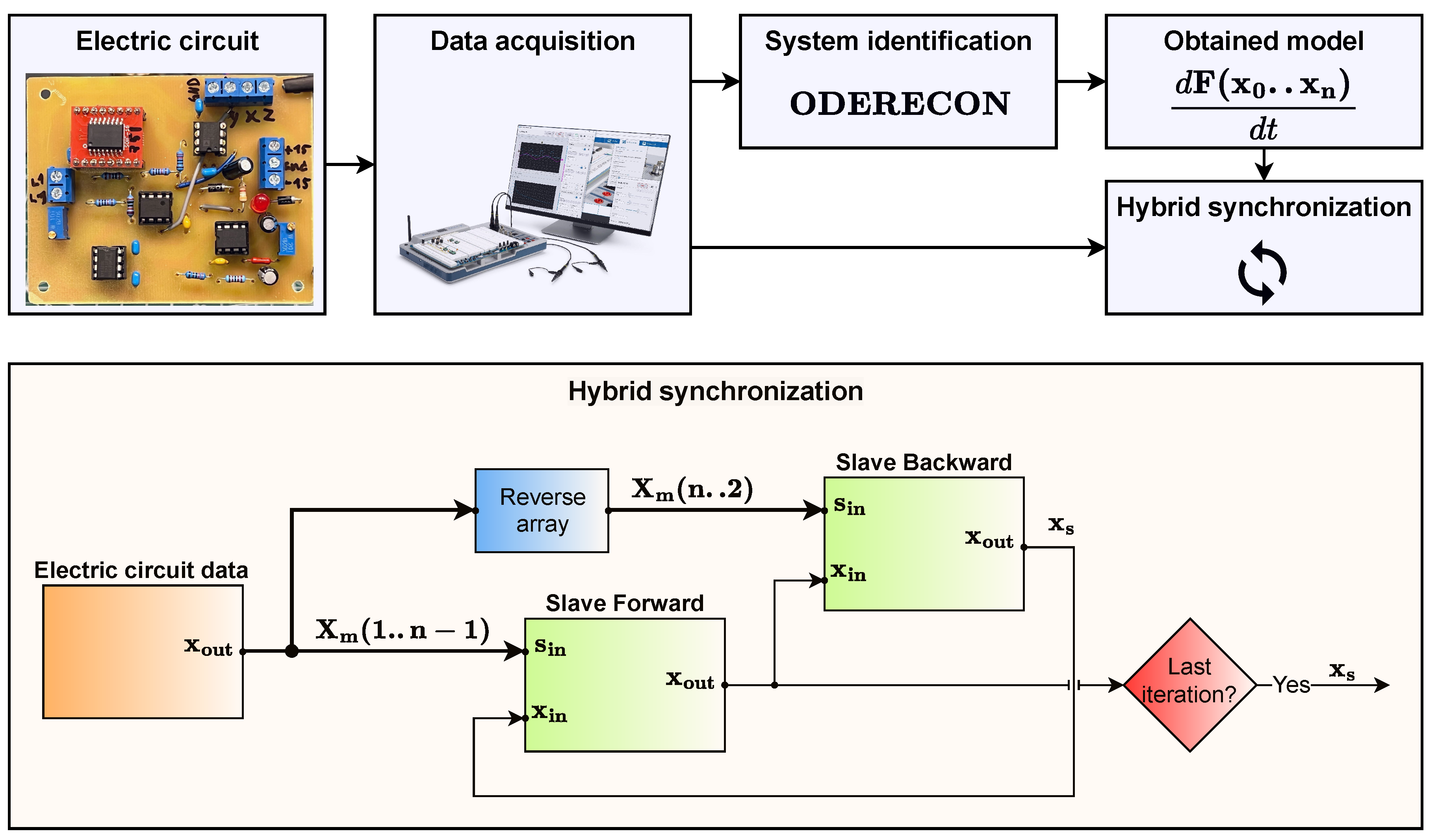
2. Materials and Methods

The chaotic Sprott Case B system is defined by the following ordinary differential equations (ODEs):

$$\begin{array}{cc}\hfill & {\dot{x}}_m=a{y}_m{z}_m\hfill \\ \hfill & {\dot{y}}_m=b{x}_m-c{y}_m\hfill \\ \hfill & {\dot{z}}_m=d-e{x}_m{y}_m.\hfill \end{array}$$

(1)

Here, the subscript denotes that these equations refer to the master system. Unlike in the original form [28], we introduce the following additional parameters: $a=0.5$, $b=1.6$, $c=1.5$, $d=1$, and $e=1$. The slave system coupled with the master systems described by the Equation (1) is as follows:

$$\begin{array}{cc}\hfill & {\dot{x}}_s=a{y}_s{z}_s+u_x;\hfill \\ \hfill & {\dot{y}}_s=b{x}_s-c{y}_s+u_y;\hfill \\ \hfill & {\dot{z}}_s=d-e{x}_s{y}_s+u_z.\hfill \end{array}$$

(2)

The simplest control law is the proportional control

$$\begin{array}{cc}\hfill & u_x=k_x{e}_x;\hfill \\ \hfill & u_y=k_y{e}_y;\hfill \\ \hfill & u_z=k_z{e}_z,\hfill \end{array}$$

(3)

where

$$\begin{array}{cc}\hfill & e_x=x_m-x_s;\hfill \\ \hfill & e_y=y_m-y_s;\hfill \\ \hfill & e_z=z_m-z_s,\hfill \end{array}$$

and $k_x$, $k_y$, and $k_z$ are coefficients determining the coupling strengths of synchronization by each variable. Setting any of the coupling coefficients to zero, one may perform synchronization by only one or two variables. The more advanced control law is given by the following equations:

$$\begin{array}{cc}\hfill & u_x=a(y_m{z}_m-y_s{z}_s)+k_x{e}_x;\hfill \\ \hfill & u_y=b{e}_x-c{e}_x+k_y{e}_y;\hfill \\ \hfill & u_z=e(x_s{y}_s-x_m{y}_m)+k_z{e}_z.\hfill \end{array}$$

(4)

Adaptive synchronization is a type of synchronization when some parameters of the master system are uncertain, and an additional controller is utilized to find their exact parameters. The equation of the update rules for the unknown parameters is given as follows:

$$\begin{array}{cc}\hfill & \dot{a}=y_m{z}_m{e}_x;\hfill \\ \hfill & \dot{b}=x_m{e}_y;\hfill \\ \hfill & \dot{c}=-y_m{e}_y;\hfill \\ \hfill & \dot{d}=e_z;\hfill \\ \hfill & \dot{e}=-x_m{y}_m{e}_z,\hfill \end{array}$$

(5)

The convergence of Equation (2) can be verified by Lyapunov analysis. Let us denote the errors between the updated slave coefficients and the master coefficients as

$$\begin{array}{cc}\hfill & e_a=a_m-a_s;\hfill \\ \hfill & e_b=b_m-b_s;\hfill \\ \hfill & e_c=c_m-c_s;\hfill \\ \hfill & e_d=d_m-d_s;\hfill \\ \hfill & e_e=e_m-e_s,\hfill \end{array}$$

(6)

where $a_m$, $b_m$, $c_m$, $d_m$, and $e_m$ are the values of the parameters in the master system, and $a_s$, $b_s$, $c_s$, $d_s$, and $e_s$ are updated parameters of the slave system. So, the error derivatives read as

$$\begin{array}{cc}\hfill & {\dot{e}}_x=a_m{y}_m{z}_m-a_s{y}_s{z}_s-u_x;\hfill \\ \hfill & {\dot{e}}_y=b_m{x}_m-c_m{y}_m-b_s{x}_s+c_s{y}_s-u_y;\hfill \\ \hfill & {\dot{e}}_z=d_m-e_m{x}_m{y}_m-d_s+e_s{x}_s{y}_s-u_z;\hfill \\ \hfill & {\dot{e}}_a=-y_m{z}_m{e}_x;\hfill \\ \hfill & {\dot{e}}_b=-x_m{e}_y;\hfill \\ \hfill & {\dot{e}}_c=y_m{e}_y;\hfill \\ \hfill & {\dot{e}}_d=-e_z;\hfill \\ \hfill & {\dot{e}}_e=x_m{y}_m{e}_z,\hfill \end{array}$$

(7)

Recall that the second Lyapunov method for stability consists of finding a function $V\left(t\right)$ such that $V\left(t\right)=0$ for $t=0$, $V\left(t\right)\ne 0$ for $t\ne 0$, and $dV\left(t\right)/dt\le 0$ for all $t\ne 0$. Once this function exists, a certain system is Lyapunov-stable. Let us consider the following Lyapunov candidate:

$$V\left(t\right)={\displaystyle \frac{1}{2}}(e_x^2+e_y^2+e_z^2+e_a^2+e_b^2+e_c^2+e_d^2+e_e^2)={\displaystyle \frac{1}{2}}\sum _i{e}_i^2.$$

If any of $e_i\ne 0$, $V\left(t\right)$ is strictly positive. Let us take the derivative of this function as follows:

$$\begin{array}{cc}\hfill {\displaystyle \frac{dV}{dt}}=\sum _i{\displaystyle \frac{\partial V}{\partial e_i}}{\displaystyle \frac{d{e}_i}{dt}}& =-k_x{e}_x^2-k_y{e}_y^2-k_z{e}_z^2+a_s(y_m{z}_m-yz)e_x+b_s{e}_x{e}_y-c_s{e}_x{e}_y\hfill \\ & \hfill +d_s{e}_z-e_s(x_m{y}_m-x_s{y}_s)e_z=e_x{\dot{e}}_x+e_y{\dot{e}}_y+e_z{\dot{e}}_z{|}_{e_j=0,j\in \{a,b,c,d,e\}}.\end{array}$$

(8)

Equation (8) guarantees the convergence of the master and slave systems with the parameter adaptation laws (6) if convergence is possible in similar systems. Expanding this further for systems with similar parameters, one can obtain

$$\begin{array}{cc}\hfill {\displaystyle \frac{dV}{dt}}=& e_x{\dot{e}}_x+e_y{\dot{e}}_y+e_z{\dot{e}}_z=\hfill \\ \hfill & e_x(a_s(y_m{z}_m-yz)+u_x)+e_y(b_s{e}_x-c_s{e}_y+u_y)+e_z(e_s(-x_m{y}_m+x_s{y}_s)+u_z).\hfill \end{array}$$

(9)

One can see that the control law (3) may yield $dV/dt<0$ for sufficiently large $k_i$, and when the control law (4) is used, the derivative (9) becomes exactly

$$\begin{array}{c}\hfill {\displaystyle \frac{dV}{dt}}=-k_x{e}_x^2-k_y{e}_y^2-k_z{e}_z^2\le 0,\end{array}$$

(10)

which immediately indicates the convergence between the slave and the master systems.

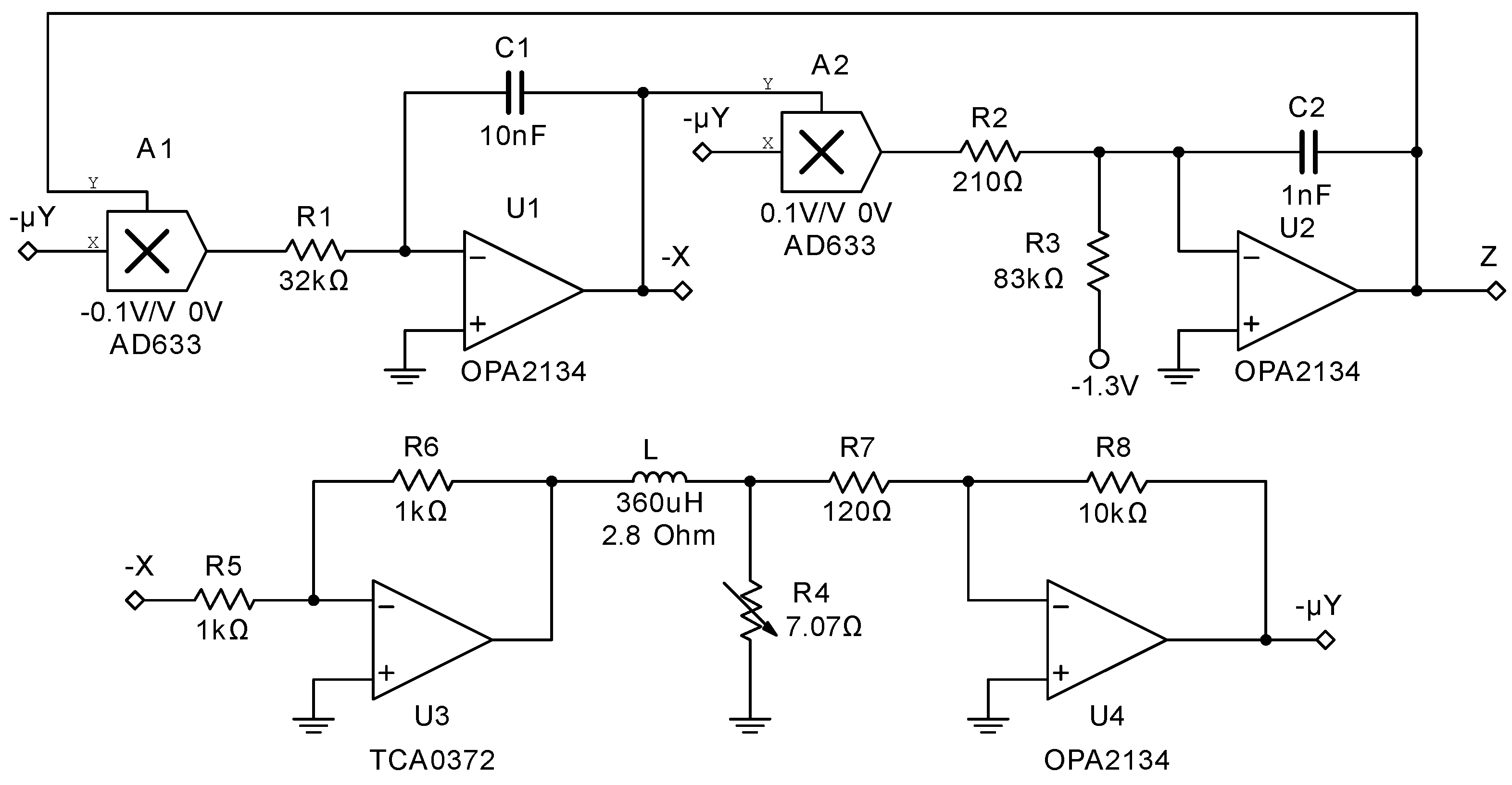
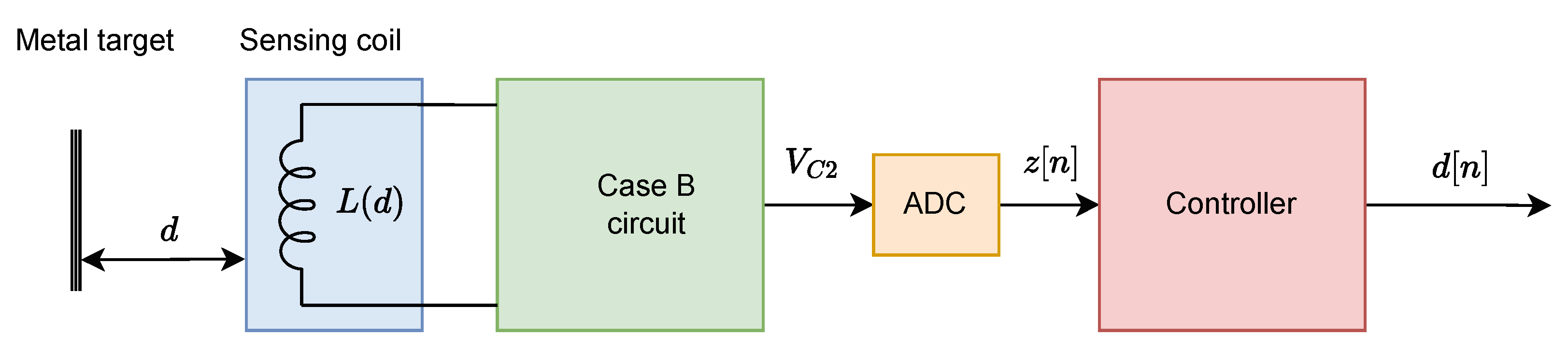
2.1. Circuit Implementation and Identification

In this subsection, we reconstruct a system from a time series representing the Sprott Case B chaotic oscillator implemented in a physical circuit based on the original Equation (1). The chaotic circuit diagram is presented in Figure 1, and a photo of its physical implementation is given in Figure 2. The circuit dynamics can be described by the following equations:

$$\begin{array}{cc}\hfill \dot{x}& {\displaystyle =\frac{\mu }{10C_1{R}_1}yz}\hfill \\ \hfill L\dot{y}& =x-(R_4+R_L)y\hfill \\ \hfill \dot{z}& {\displaystyle =-\frac{V}{C_2{R}_3}-\frac{\mu }{10C_2{R}_2}xy.}\hfill \end{array}$$

(11)

All values of the circuit elements are given in Figure 1. In Equation (11), the voltages on capacitors $C_1$ and $C_2$ correspond to variables x and z, respectively, and the current in the coil L corresponds to the variable y. To obtain the exact value of y, the parameter

$$\mu ={\displaystyle \frac{R_4{R}_7}{R_6}}$$

is introduced, denoting the transfer coefficient of the current-sensing circuit including the resistor $R_4$ and an inverting amplifier on $U_4$. The divider 10 in the first and third lines of (11) is the transfer coefficient of the analog multipliers $A_1$ and $A_2$. The bipolar power supply $\pm 15$ V is utilized. The integrators were made using OPA2134 operational amplifiers, and the analog multipliers AD633 were used. An additional operational amplifier TCA0372 was used to provide high enough current in the sensing coil L.

Figure 2 shows that the circuit is designed to be used with an external sensing cup core coil, which is typical for inductive limit switches and distance sensors. The coil is fixed in a holder and is capable of detecting metal targets approximating to it. Eddy currents induced in the metal plate influence the coil inductance and thus affect the chaotic dynamics of the whole circuit depending on the distance to the plate and the metal it is made of. In practical applications, parameter L may be found using adaptive synchronization between the circuit and its model.

The second line of (11) shows how L can be estimated directly from the circuit phase variables, which is a faster but less accurate alternative to adaptive synchronization. The general form of this line can be obtained as

$$L\dot{y}=f_y(x,y,z),$$

(12)

so that

$$L={\displaystyle \frac{f_y(x,y,z)}{\dot{y}}},\left|\dot{y}\right|>\epsilon ,$$

(13)

where $\epsilon$ is a small value which ensures that the L in (13) is estimated correctly. Having estimated L, the distance is found using a simple formula. It is known that the distance to the target and the inductance L in the circuit are related to each other through a nearly hyperbolic law [29]:

$$L\left(d\right)={\displaystyle \frac{k}{d}}+L_0,$$

(14)

where k and $L_0$ are estimated during the sensor calibration. This equation allows for finding d once L is known as follows:

$$d={\displaystyle \frac{k}{L-L_0}}.$$

(15)

Substituting (13) into (15) yields

$$d={\displaystyle \frac{k\dot{y}}{f_y(x,y,z)-L_0\dot{y}}},$$

(16)

which is more computationally stable than (13), since the derivative $\dot{y}$ (which is in practice estimated numerically) is in the numerator.

To perform identification of the real circuit shown in Figure 2, the recorded data of all three phase variables were used in the algorithm ODERECON for the reconstruction of the governing equations. This algorithm is described in detail in [19]. Here, we briefly outline its main steps.

In this algorithm, we reconstruct the system as an autonomous polynomial dynamical system as follows:

$$\dot{\mathbf{x}}=\mathbf{F}\left(\mathbf{x}\right),$$

where $\mathbf{x}={(x_1,x_2,\dots ,x_n)}^{\top }$ is the phase variable vector, and each entry of the derivative function ${\mathbf{F}}_i\left(\mathbf{x}\right)$ is a polynomial defined as

$${\mathbf{F}}_i\left(\mathbf{x}\right)=\sum _{k=1}^L{h}_k{\tau }_k\left(\mathbf{x}\right),$$

(17)

where L is the number of monomials building up the function, and $h_k$ is a coefficient of the k-th monomial. Under the monomial, we understand a product of variables as

$${\tau }_k\left(\mathbf{x}\right)=\prod _{j=1}^d{x}_j^{{\alpha }_{kj}},$$

where d is the number of variables, ${\alpha }_{kj}$ is the j-th variable degree, and $\sum {\alpha }_{kj}$ is an overall degree of the monomial.

Let the overall dataset be represented as the matrix $\mathbb{X}={({\mathbf{x}}_0,{\mathbf{x}}_1,\dots ,{\mathbf{x}}_n)}^{\top }$, where ${\mathbf{x}}_i=\mathbf{x}\left(t_i\right)$, and the derivatives of $\mathbf{x}$ are given in a matrix $\mathbb{Y}={({\mathbf{y}}_0,{\mathbf{y}}_1,\dots ,{\mathbf{y}}_n)}^{\top }$, where ${\mathbf{y}}_i={\dot{\mathbf{x}}}_i$. After obtaining these matrices, we can estimate the matrix of monomial values on $\mathbb{X}$ as

$$E_i\left(\mathbb{X}\right)=\left(\begin{array}{cccc}{\tau }_{k_1}\left({\mathbf{x}}_1\right)& {\tau }_{k_2}\left({\mathbf{x}}_1\right)& \cdots & {\tau }_{k{L}_i}\left({\mathbf{x}}_1\right)\\ {\tau }_{k1}\left({\mathbf{x}}_2\right)& {\tau }_{k2}\left({\mathbf{x}}_2\right)& \cdots & {\tau }_{k{L}_i}\left({\mathbf{x}}_2\right)\\ ⋮& ⋮& \ddots & ⋮\\ {\tau }_{k1}\left({\mathbf{x}}_n\right)& {\tau }_{k2}\left({\mathbf{x}}_n\right)& \cdots & {\tau }_{k{L}_i}\left({\mathbf{x}}_n\right)\end{array}\right).$$

(18)

Write down all coefficients of the monomials in $f_i$ as a vector defined as

$${\mathbf{h}}_i=\left(\begin{array}{c}{h}_{i_1}\\ h_{i_2}\\ ⋮\\ h_{i_L}\end{array}\right).$$

(19)

After that, Equation (17) obtains a compact matrix form defined as

$${\mathbf{y}}_i=E_i{\mathbf{h}}_i.$$

(20)

The system reconstruction problem is to find such ${\mathbf{h}}_i$ that Equation (17) minimizes the least square error between the reconstructed function and actual values of derivatives:

$${({\mathbf{y}}_i-E_i{\mathbf{h}}_i)}^{\top }({\mathbf{y}}_i-E_i{\mathbf{h}}_i)\to min.$$

The solution of (20) using the ordinary least squares method (LSM) is

$${\mathbf{h}}_i={\left(E_i^{\top }{E}_i\right)}^{-1}\left(E_i^{\top }{\mathbf{y}}_i\right).$$

(21)

The value ${\mathbf{h}}_i$ can be obtained from the overall dataset or from different points of the signal, but the general idea of solving the identification problem remains similar in both cases.

For practical purposes, some further steps were added. First, data $\mathbb{X}$ were filtered to make them smoother and remove high-frequency noise. Derivatives $\mathbb{Y}$ were obtained using numerical integration, where fourth- or higher-order methods were preferred. Then, the approximate Buchberger-Möller algorithm was performed to eliminate monomials that could cause ill posedness of Equation (21). Then, the solution could be sparsified using a special procedure delMinorTerms if needed. Nevertheless, a dense representation is preferable for achieving the most accurate result.

To estimate the error of the system reconstruction, an approach of estimating the synchronization error was applied. According to the unifying definition of synchronization by R. Brown and L. Kocarev [24], suppose that there are two coupled dynamical systems ${\mathsf{\Phi }}_x(t,\mathbf{x},\mathbf{y})$ and ${\mathsf{\Phi }}_y(t,\mathbf{y},\mathbf{x})$, which have properties $\mathbf{g}\left(\mathbf{x}\right)$ and $\mathbf{g}\left(\mathbf{y}\right)$. They are synchronized on the trajectory $\varphi \left({\mathbf{z}}_0\right)$, where ${\mathbf{z}}_0={({\mathbf{x}}_0,{\mathbf{y}}_0)}^{\top }$, if there exists a certain time-independent function $\mathbf{h}$ such that

$$\parallel \mathbf{h}\left(\mathbf{g}\right(\mathbf{x}),\mathbf{g}(\mathbf{y}\left)\right)\parallel =0.$$

Taking $\mathbf{g}\left(\mathbf{x}\right)=\mathbf{x}\left(t\right)$, $\mathbf{g}\left(\mathbf{y}\right)=\mathbf{y}\left(t\right)$, and $\mathbf{h}$ as the synchronization error between ${\mathsf{\Phi }}_x(t,\mathbf{x},\mathbf{y})$ and the identical auxiliary function ${\mathsf{\Psi }}_x(t,\mathbf{x},\mathbf{y})$ yields the generalized synchronization [30]. The error between two nearly similar systems $\mathbf{e}\left(t\right)$ can serve as the estimate of their proximity, with a particular case ${\mathsf{\Phi }}_x(t,\mathbf{x},\mathbf{y})\equiv {\mathsf{\Phi }}_y(t,\mathbf{y},\mathbf{x})$ if ${lim}_{t\to \infty }\parallel \mathbf{e}\left(t\right)\parallel =0$. The estimate $\mathbf{e}\left(t\right)$ is time-dependent, but taking the root mean square of its norm $RMS(\parallel \mathbf{e}(t)\parallel )$ allows for obtaining a number characterizing the distance between ${\mathsf{\Phi }}_x(t,\mathbf{x},\mathbf{y})$ and ${\mathsf{\Phi }}_y(t,\mathbf{y},\mathbf{x})$ on the entire time interval. This estimation is relative and depends on the synchronization method and the coupling strength but allows one to distinguish two slave systems, ${\mathsf{\Psi }}_y(t,\mathbf{y},\mathbf{x})$ and ${\mathsf{\Phi }}_y(t,\mathbf{y},\mathbf{x})$ synchronized with the master ${\mathsf{\Phi }}_x(t,\mathbf{x})$, if the synchronization parameters in these slave systems are similar.

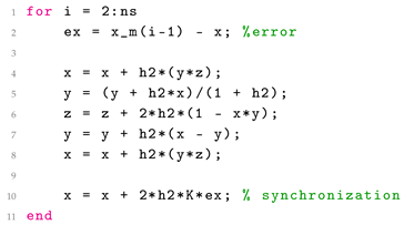
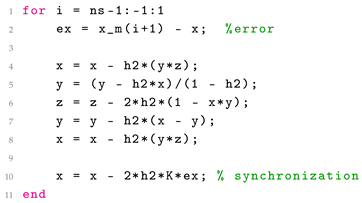
2.2. Time-Reversible Synchronization

To perform the time-reversible synchronization between the analog and digital systems, a special routine was proposed, as is shown in Figure 3. First, the signal from the electronic circuit was acquired using special hardware. Then, the ODERECON algorithm was run to obtain a reconstructed model, as described above. Finally, the fragment of newly acquired data could be used in a hybrid synchronization process.

The hybrid synchronization is detailed in Figure 3 on the bottom panel. The discrete fragment of the master signal ${\mathbf{X}}_{\mathbf{m}}=({\mathbf{x}}_1,{\mathbf{x}}_2\dots {\mathbf{x}}_n)$ obtained from the output ${\mathbf{x}}_{out}$ of the data acquisition system was supplied into a slave model with a forward time direction. After processing $n-1$ samples, the obtained new state of the slave system ${\mathbf{x}}_s$ was used as an initial state in the synchronization in the backward direction, when the time step was taken with a negative sign, and the master signal was reversed as if the process went back in time. An output of the overall synchronization process is the state of the slave system at the last point after the terminal forward step.

The theoretical background behind the time-reversible synchronization can be briefly given as follows. Let us consider a system described by the following autonomous ordinary differential equation:

$${\dot{\mathbf{x}}}_m\left(t\right)=f\left({\mathbf{x}}_m\left(t\right)\right).$$

The solution ${\mathbf{X}}_{\mathbf{m}}$ on a certain time interval is known. Let ${\mathbf{x}}_s$ denote the phase vector of the slave system. Then, the equation of the slave system reads as

$${\dot{\mathbf{x}}}_s=f\left({\mathbf{x}}_s\right)+K_f\mathbf{e},$$

(22)

where $\mathbf{e}=\mathbf{x}-{\mathbf{x}}_s$ is the synchronization error, and $K_f$ is a (semi-)positive definite matrix. In practical applications, $K_f$ contains a single diagonal element corresponding to the recorded variable. The equation for the time-reversed system is

$${\dot{\mathbf{x}}}_s=-(f\left({\mathbf{x}}_s\right)+K_b\mathbf{e}),$$

(23)

where the minus sign appears due to the reverse direction in time, and $K_b$ is a (semi-)negative definite matrix. The synchronization signal for the forward phase contains all data points except the last one, ${\mathbf{X}}_f=({\mathbf{x}}_1,{\mathbf{x}}_2\dots {\mathbf{x}}_{n-1})$, and the synchronization signal for the backward phase starts from the second point, ${\mathbf{X}}_b=({\mathbf{x}}_n,{\mathbf{x}}_{n-1}\dots {\mathbf{x}}_2)$, as Figure 3 illustrates. The iteration number is a subject of experimental adjustment.

Let us verify the proposed synchronization method using the Lyapunov stability theory. The Lyapunov candidate function $V\left(t\right)$ is usually taken in the form

$$V\left(t\right)={\displaystyle \frac{1}{2}}{\mathbf{e}}^{\top }H\mathbf{e},$$

where H is a positive definite matrix. Supposing its equality to the identity matrix $H=I$, its derivative is

$$\dot{V}\left(t\right)={\mathbf{e}}^{\top }\dot{\mathbf{e}}=\mathcal{F}(t,\mathbf{x},\mathbf{e})-K_f{\mathbf{e}}^{\top }\mathbf{e},$$

(24)

where $\mathcal{F}(t,\mathbf{x},\mathbf{e})$ is a certain limited function, and for sufficiently large values $K_f{\mathbf{e}}^{\top }\mathbf{e}$, we obtain $\dot{V}\left(t\right)\le 0$. This implies that $K_f$ is (semi-)positive definite. For the reverse direction of synchronization, rewrite (24) so that it reads as

$$\dot{V}(-t)=-\dot{V}\left(t\right)=-\mathcal{F}(t,\mathbf{x},\mathbf{e})+K_b{\mathbf{e}}^{\top }\mathbf{e},$$

so the synchronization matrix $K_b$ at the backward phase should be (semi-)negative definite to provide $\dot{V}(-t)\le 0$.

The finite-difference implementation of the time-reversible synchronization after applying the integration method to the system (22) yields

$${\mathbf{x}}_{n+1}={\mathbf{x}}_n+h{\mathsf{\Phi }}_h({\mathbf{x}}_i,K_f),i\in \mathbb{Z},i\le n+1,$$

and after applying to (23), it yields

$${\mathbf{x}}_{n-1}={\mathbf{x}}_n-h{\mathsf{\Phi }}_{-h}({\mathbf{x}}_i,-K_b),i\in \mathbb{Z},i\ge n-1,$$

which requires the time reversibility of the integration method ${\mathsf{\Phi }}_h^{-1}={\mathsf{\Phi }}_{-h}$, once $-K_b=K_f$, and the system is locally reversible within the given time interval. However, as we showed in [27], the reversibility of the system is not necessary to make the time-reversible synchronization work.

For the Sprott Case B system, the finite-difference scheme obtained by applying the second-order CD method for the forward step reads as given below. Here, the variable h2 = h/2 denotes the half integration step, and the variables x, y, z contain phase variables. The array x_m contains the master signal by the variable x, K is the synchronization coefficient, and ns is the number of points in the master signal fragment.

The finite-difference scheme for the backward step is as follows:

Note that the synchronization coefficient at the backward step is negative, while at the forward step, it is positive.

Time-reversible synchronization allows for recovering the system state having only a short fragment of the master system trajectory of length $ns$, which can be as short as only a few points, since the integration method theoretically requires only two points per step to run. However, usually $ns$ can be selected around 100 if the discretization rate allows.

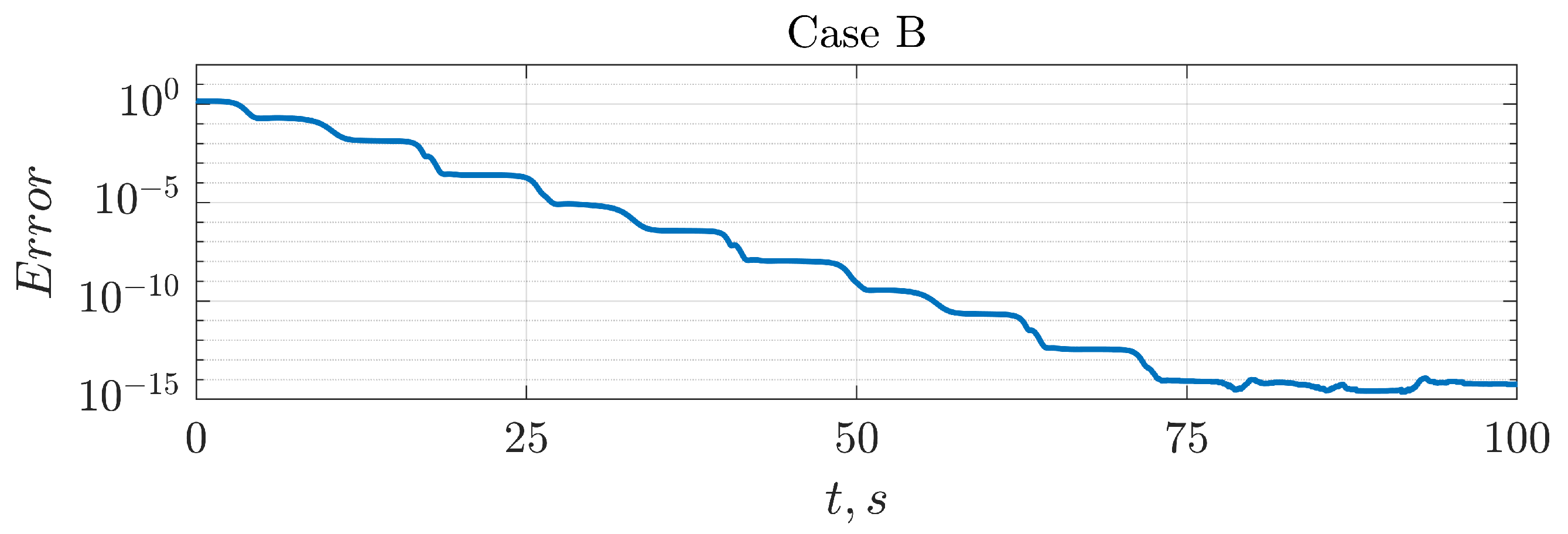
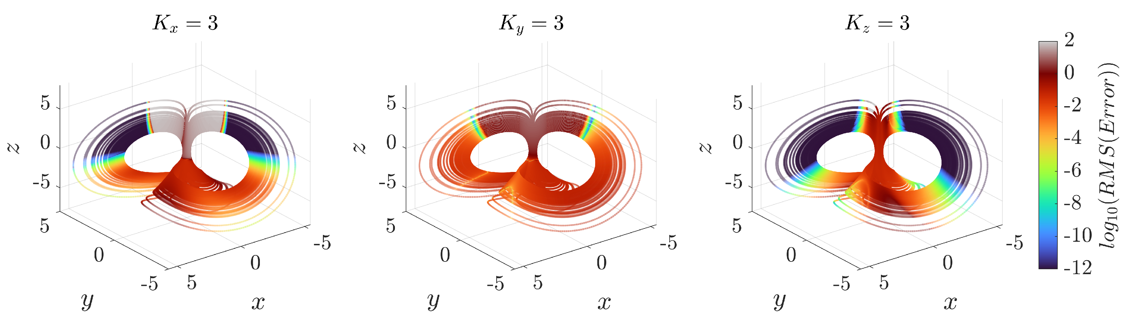
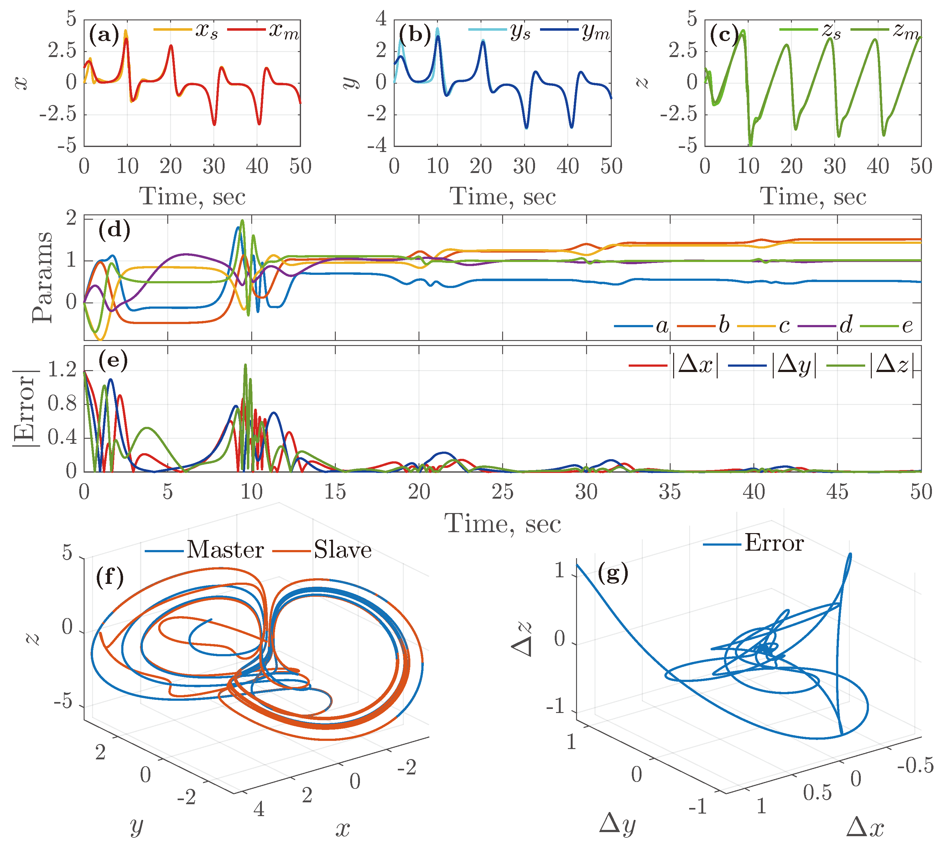
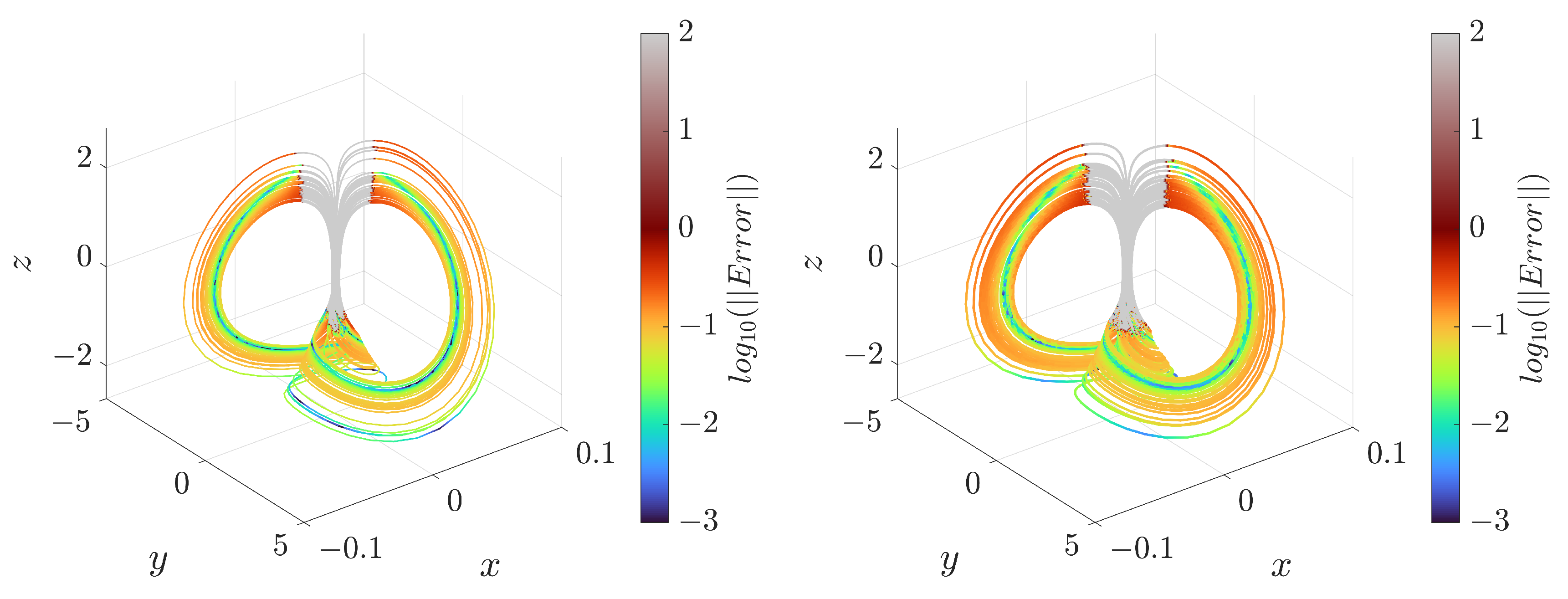
3. Experimental Results

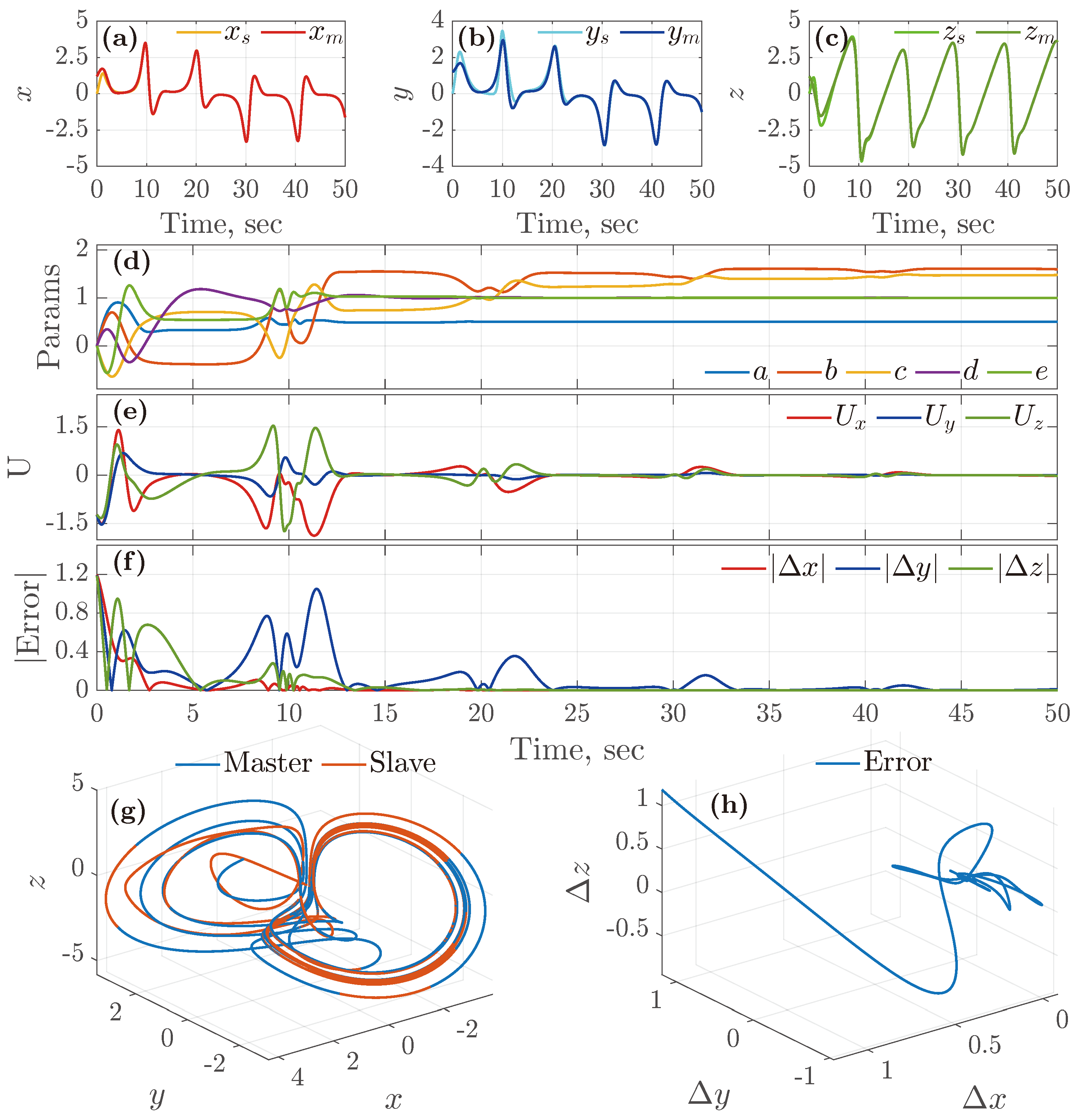
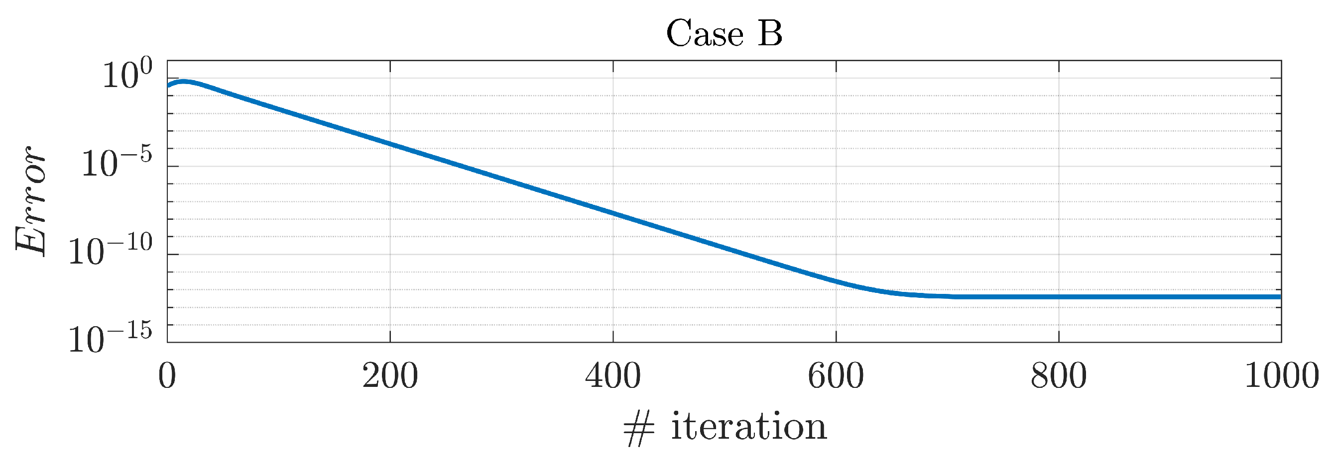
3.1. Numerical Experiments

In all experiments with identical and adaptive synchronization, the initial conditions for the master system were used as $x_0=-2,y_0=-4,z_0=10$ and for the slave system as $x_0=6,y_0=5,z_0=5$. For time-reversible synchronization, the initial conditions for the slave systems were chosen at the origin $x_0=0,y_0=0,z_0=0$.

In experiments with identical and adaptive synchronization, the coefficient of $k_x=3$ was empirically chosen, while two other coupling strengths were set to zero. The synchronization error of two coupled systems with identical synchronization by the variable x is demonstrated in Figure 4. It is important to note that the identical synchronization is only effective using the x variable, while the time-reversible method is capable of working using any of the three variables, as illustrated in Figure 5. The color of the point on the attractor in Figure 5 shows the error achieved after 200 forward–backward iterations when 1 s of the master system signal started from this point. For example, when systems are synchronized with the variable x, the initial conditions in the dark blue zone yield the final error of order ${10}^{-12}$, and the initial conditions in the gray zone yield a loss of stability of the slave system during the synchronization process. The initial conditions in the red and orange zones lead to very low convergence or stop the convergence at high errors. Green zones correspond to intermediate levels of error, but only blue regions guarantee full convergence.

Numerical experiments with adaptive synchronization show that under other similar conditions, the advanced adaptation law (4) outperformed the proportional control law (3) in terms of the synchronization rate, as we illustrate below. Figure 6 shows the synchronization error for adaptive synchronization with the proportional law (3) in the Case B system displayed at the top. The bottom pane shows changes in parameter values over time on the slave side. The top pane of Figure 7 shows the synchronization error for adaptive synchronization with the advanced law (4). The middle panel also shows changes in the parameter values over time on the slave side. In both cases, $k_x=k_y=k_z=3$. The bottom panel illustrates the time domain of the master and slave signal using the y variable. After 30 s, the error could not be evaluated by the naked eye, but in fact, it decayed for more than 200 s before it reached the level of the machine epsilon. Comparing the obtained results, we see the better performance of the advanced law. It also produced less overshooting and less aggressive control.

The results of the time-reversible control are illustrated in Figure 8. In this figure, the horizontal axis displays the number of iterations rather than time, and the vertical axis gives the error norm at the last point of the forward step. The initial condition for the master system was used, ${\mathbf{x}}_{m0}={(1,1,1)}^{\top }$, and synchronization was started after $205.534$ s of transient time. The synchronization coefficients were set to $K_f=3,K_b=-3$, and the length of the master system signal (synchronization window) was 1 s, so one iteration would correspond to one second if this was the ordinary identical synchronization. However, in fact, one needs only 1 s of the master system signal to achieve the level of synchronization error below ${10}^{-12}$.

Table 1. Comparison of synchronization types according to minimal synchronization errors.

Type	Iterations	N Points
		15	30	100
Pecora–Carroll	−	1.787	1.491	0.681
Adaptive	−	1.016	0.803	0.606
Reversible	10	0.889	0.896	0.596
	100	0.836	0.532	0.018
	1000	0.45	0.027	3.962 × 10−13

summarizes the experimental results, displaying the minimal achieved error for three different synchronization types: the Pecora–Carroll synchronization, the advanced adaptive synchronization (4), and the proposed time-reversible synchronization. The experiments involved 15-, 30-, and 100-point windows of the synchronization signal, corresponding to 0.15, 0.3, and 1 s of the signal duration, respectively. In the case of the time-reversible synchronization, 10, 100, and 1000 iterations were performed. It is evident that the selection of an appropriate number of iterations for the time-reversible synchronization and the number of points in the time window resulted in a low synchronization error of order ${10}^{-13}$ (given in bold font). This level of accuracy was unattainable in the case of any other type of synchronization.

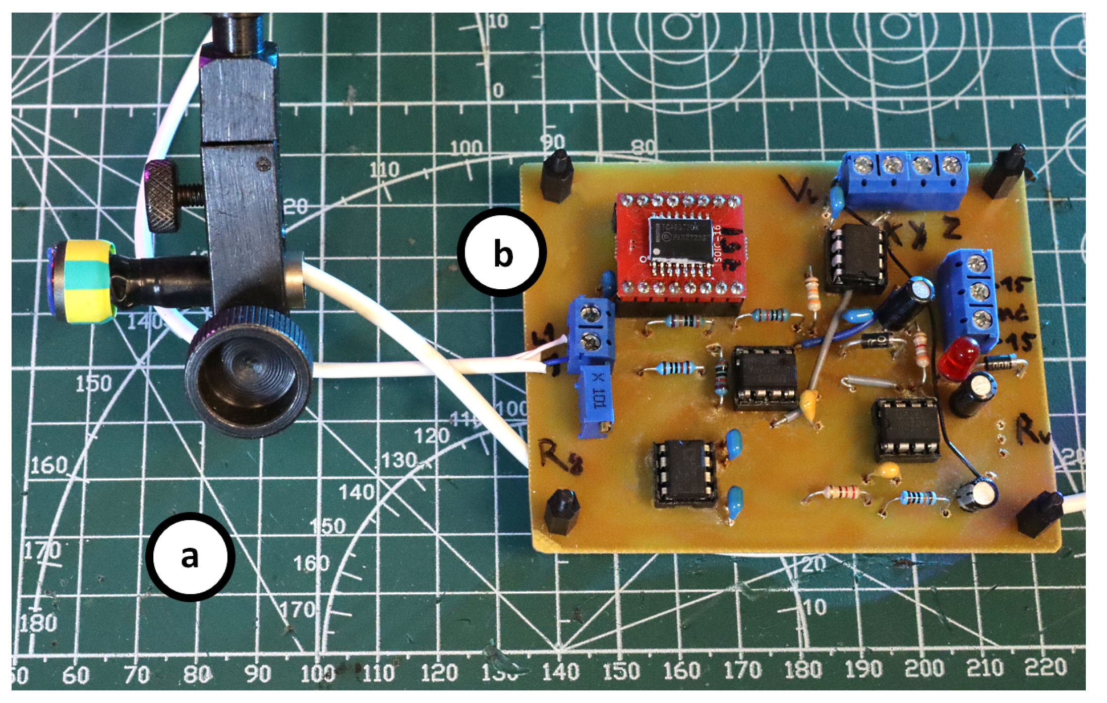
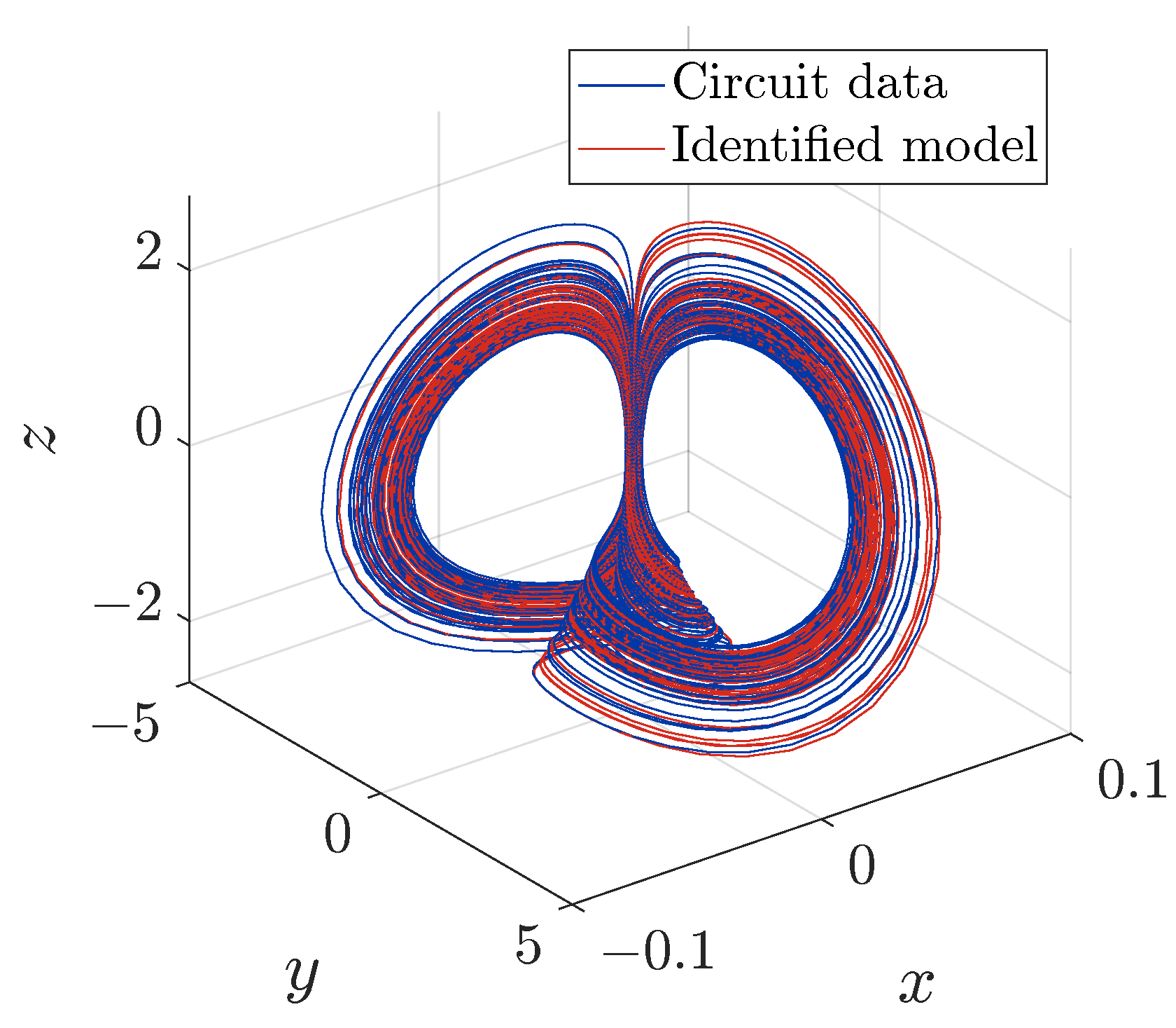
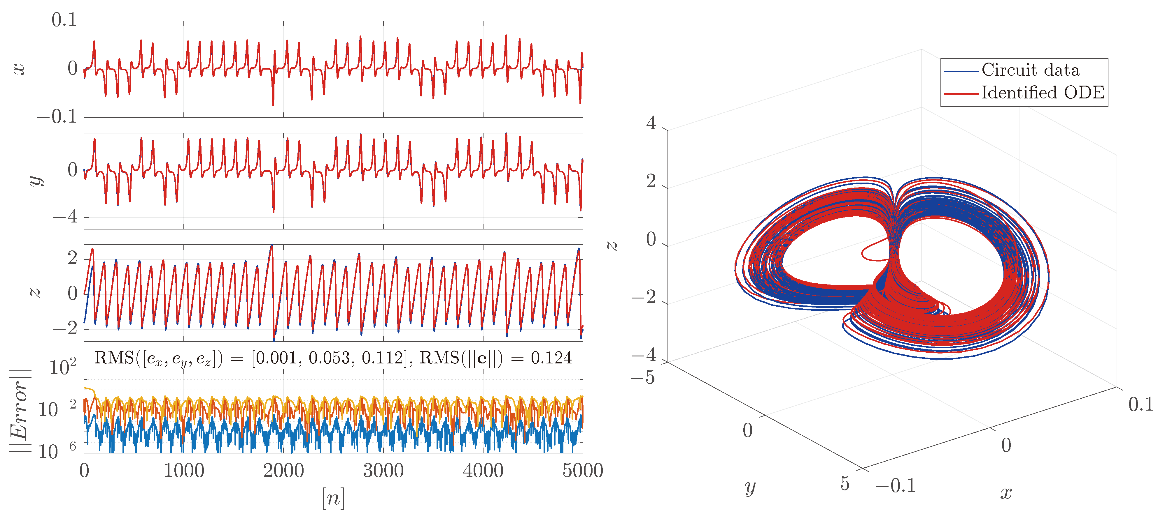
3.2. Physical Experiments

The data from the Case B circuit were recorded using the NI ELVIS III board with the discretization time step $h=6·{10}^{-6}$. Using the ODERECON algorithm, we obtained dense equations of the circuit with coefficients, which are given in

Table 2. Monomial coefficients for the identified ODE.

Monomial	$\dot{\mathit{x}}$	$\dot{\mathit{y}}$	$\dot{\mathit{z}}$
Constants
1	0.56584	−1889.7719	7294.8977
Linear terms
x	525.8895	1,631,650.7934	−15,674.7009
y	−19.1559	−28,145.5863	1030.2079
z	−1.062	−36.5299	−314.1264
Quadratic terms
$x^2$	1863.194	−428,705.5214	−3,107,210.5065
$xy$	20.2827	20,185.9366	−300,112.975
$xz$	−509.3423	−36,035.4457	−20,384.6695
$y^2$	−0.13808	−394.7372	−604.5916
$yz$	282.167	289.9596	684.9051
$z^2$	−0.24937	10.7169	−116.461
Qubic terms
$x^{2}y$	−23,687.6184	−217,773.3151	19,662.5142
$x^{2}z$	−509.2357	−986.8019	−1,050,985.1787
$x{y}^2$	265.0119	12,758.1406	752.5436
$x{z}^2$	160.1033	−7751.9336	−4795.2182
$y^3$	9.2083	−196.1558	−33.2336
$y{z}^2$	−7.5831	409.9541	218.3688

. These coefficients were rounded to 3–5 digits after the decimal point and grouped by the degree of monomials.

The comparison of the recorded data and the attractor of the obtained equations demonstrates good correspondence, as is shown in Figure 9. Here and further, the second-order CD integration method was used [27], and the emerging implicit equations were resolved using eight iterations of the simple iteration method.

While the attractors of the identified model and the circuit in Figure 9 are visually close, the exact relationship between them can be estimated using the synchronization test. In the following tests, we compared the accuracy of the physics-based model (11) and the identified model using one variable x. Selecting relatively large $K_x=$ 14,000, we obtained the dynamics, as shown in Figure 10. In the left panes of the figure, the dynamics of three variables are given and the error using three variables. In the right pane of the figure, the attractor of the original circuit and the synchronized model are shown. One sees relatively poor correspondence, with the overall RMS error being 1.947. Increasing or decreasing $K_x$ only made the RMS error even larger, resulting in overshooting for variables y and z while not even reducing the error for x.

Figure 11 corresponds to the experiment with the identified model, with the coefficients given in Table 2. The coupling strength $K_x=$ 85,000 was used, which allowed for decreasing the error to a relatively small level. In the left panes of the figure, the dynamics of the three variables are given, and the error for the three variables is sufficiently smaller in this case. The RMS error was only 0.124, which is 16 times smaller than in the case of model (11). In the right pane of the figure, the attractor of the original circuit and the synchronized model are shown, and the correspondence is visually also good.

The final experiment answers the main question of the paper: can time-reversible synchronization be used for analog-to-digital synchronization? Figure 12 shows the error of the time-reversible synchronization in the last point of the forward synchronization step after $N_{iter}=10$ iterations using $ns=50$ points of the synchronization signal for the z variable with $K_z^f=K_z^b=$ 200,000. The discretization time step was $h=6·{10}^{-6}$. The left pane of Figure 12 demonstrates the results of the time-reversible synchronization between the two identified models, and the right pane of Figure 12 illustrates the results of the time-reversible synchronization between the circuit and the identified model. The color meaning is similar to Figure 5: blue colors correspond to the initial conditions of the master system where a low error of the time-reversible synchronization was achieved, while red colors correspond to the initial conditions of the master system where the time-reversible synchronization achieved high errors. The gray color corresponds to the initial conditions of the master system where the slave system lost stability during the time-reversible synchronization. One can see a high level of equivalence between these two images. Also, the time-reversible synchronization behavior in this experiment is not similar to the Sprott Case B original model. The best-achieved error was only about ${10}^{-3}$, which is approximately the noise level, and the set of initial conditions from where this error was achieved is also much smaller: only narrow blue stripes are distinct at the attractor, while the attractor of the original model had solid blue zones, as Figure 5 shows. Nevertheless, the existence of continuous sets on the attractor where the time-reversible synchronization error is low is demonstrated, which proves the proposed idea.

4. Discussion

One possible application of the investigated Sprott Case B chaotic circuit is a chaotic distance sensor. The diagram of such a device is given in Figure 13. This sensor uses a digital controller, which acquires the variable z of the circuit through the high-precision ADC and recovers two other variables, x and y, using time-reversible synchronization and then finds the distance d through the Equation (16). Since the recovery of state variables x and y is only possible with adequate accuracy in the blue regions of the attractor shown in Figure 9, an additional estimator of the convergence of the synchronization is used to avoid excessive computations. A single ADC simplifies the circuitry and reduces manufacturing costs.

The working principle of the proposed chaotic sensor differs from previously reported devices with the same functionality [29,31,32]. Instead of estimating the features of chaotic dynamics or using adaptive synchronization, the proposed sensor is based on estimating the parameter d directly from phase variables using the Equation (16). The fact that the time-reversible synchronization requires a small amount of data allows the operating speed of this sensor to increase.

The real performance of this distance sensor can be estimated after extensive testing of the prototype and will be known in the future. Let us summarize its possible advantages over existing inductive distance sensors. First, due to the use of chaos, the proposed sensor might be more sensitive, selective, and accurate than up-to-date sensors with harmonic oscillators, like its previously reported counterparts [29,31,32]. Second, due to the use of short time sequences for distance estimation, the sampling rate of this sensor could be much faster than the sampling rates of other chaotic sensors, since it would not have to wait for exponential convergence of the synchronization process. Third, the cost of the sensor electronics would be comparable with the cost of its up-to-date counterparts, and the sensing coil would be exactly the same.

In addition chaotic sensing, fast time-reversible synchronization may find applications in automatic control systems for estimating unobservable state variables, in chaotic communication for recovering parameters of chaotic waveform generators, and in the natural sciences for recovering the dynamics of various periodic processes. A possible application in the latter field is the estimation of parameters and dynamical variables of celestial bodies, since in most cases, the only sources of data on remote objects in space are observations made on Earth and nearby.

Also, let us summarize the limitations of the proposed time-reversible approach. First, and most importantly, the time-reversible synchronization algorithm is sensitive to its parameters: the window time $WT$, number of iterations N, and initial conditions ${\mathbf{x}}_0$. The latter is illustrated by various colored areas in Figure 5 and Figure 12: based on some initial conditions from the attractor, the algorithm easily achieved the complete synchronization, but with the other initial conditions, the synchronization failed. The latter should be detected and processed in any practical application, which may reduce the performance of the instrument based on time-reversible synchronization. Second, the algorithm is computationally demanding, and some high-frequency applications may need powerful digital signal processors to run it. Third, this algorithm is easily implemented in software, but physical implementation, e.g., in a circuit, might be complicated.

The most straightforward potential area for improvement is designing an algorithm for the practical application of time-reversible synchronization. Also, extreme conditions of work are still not investigated: how many points are needed to guarantee the convergence of the algorithm for a particular system? Also, applying some advanced controllers, such as a PID controller, may additionally improve the convergence rate.

5. Conclusions

The main idea of this study was to discover whether it is possible to implement time-reversible synchronization between a model and a physical system when the only information about a single state variable is available. This problem arises from the difference between the complex dynamics of real-world systems and their simplified models commonly used in engineering applications, especially due to the presence of noise, which is not strictly Gaussian. In our study, we clearly demonstrated that polynomial reconstruction of the governing equations can achieve a high degree of correspondence between the analog circuit and its model. The example of the Sprott Case B chaotic circuit convincingly demonstrates the possibility of time-reversible analog-to-digital synchronization. In this experiment, the real data synchronize with the identified model with an accuracy of order ${10}^{-3}$ (approximate noise level) using only 50 points. Without identification, complete synchronization between the circuit and the digital model is not possible.

In a set of numerical experiments, we showed that the feasible length of the master system signal required to achieve the desired synchronization error was much smaller for the time-reversible synchronization in comparison with the Pecora–Carroll and adaptive types of synchronization. In experiments with the original model (1), the identical synchronization with dissipative coupling required about 6000 points (60 s) of the master signal to reach the ${10}^{-12}$ error level. Adaptive synchronization required more than 20,000 points (200 s of simulation time) to reach the same error level. Using time-reversible synchronization, only 100 points (1 s) were needed to achieve the required level of synchronization. Table 1 summarizes the minimal achieved error level in numerical simulation, revealing that only the proposed approach allows for achieving complete synchronization using only a small fragment of the synchronization signal.

Further research will focus on the practical implementation of chaotic sensors with time-reversible synchronization, the prototyping of chaotic communication systems, and the further investigation of time-reversible synchronization in nonlinear dynamics. For example, adaptive time-reversible synchronization will be developed and investigated. Another important question is whether time-reversible synchronization is possible on trajectories that are not lying on the attractor. To date, no theory explains the connection between the time-reversible synchronization performance and other properties of the attractor, such as hyperbolicity and local Lyapunov spectra. These questions are of great interest and will be investigated in the future.

References

1. Pecora, L.M.; Carroll, T.L. Synchronization in chaotic systems. Phys. Rev. Lett. 1990, 64, 821. [Google Scholar] [CrossRef] [PubMed]
2. Tsimring, L.S.; Sushchik, M.M. Multiplexing chaotic signals using synchronization. Phys. Lett. A 1996, 213, 155–166. [Google Scholar] [CrossRef]
3. Dmitriev, A.; Hasler, M.; Panas, A.; Zakharchenko, K. Basic principles of direct chaotic communications. In Synchronization: Theory and Application; Springer: Berlin/Heidelberg, Germany, 2003; pp. 41–63. [Google Scholar]
4. Babajans, R.; Cirjulina, D.; Capligins, F.; Kolosovs, D.; Litvinenko, A. Synchronization of Analog-Discrete Chaotic Systems for Wireless Sensor Network Design. Appl. Sci. 2024, 14, 915. [Google Scholar] [CrossRef]
5. Klein, E.; Mislovaty, R.; Kanter, I.; Kinzel, W. Public-channel cryptography using chaos synchronization. Phys. Rev. E Stat. Nonlinear Soft Matter Phys. 2005, 72, 016214. [Google Scholar] [CrossRef]
6. Andreev, A.V.; Maksimenko, V.A.; Pisarchik, A.N.; Hramov, A.E. Synchronization of interacted spiking neuronal networks with inhibitory coupling. Chaos Solitons Fractals 2021, 146, 110812. [Google Scholar] [CrossRef]
7. Hsiao, F.H.; Chang, S.W. Integrating rc6 stream cipher to a chaotic synchronization system. IEEE Access 2024, 12, 26308–26323. [Google Scholar] [CrossRef]
8. Karawanich, K.; Chimnoy, J.; Khateb, F.; Marwan, M.; Prommee, P. Image cryptography communication using FPAA-based multi-scroll chaotic system. Nonlinear Dyn. 2024, 112, 4951–4976. [Google Scholar] [CrossRef]
9. Feng, W.; Yang, J.; Zhao, X.; Qin, Z.; Zhang, J.; Zhu, Z.; Wen, H.; Qian, K. A novel multi-channel image encryption algorithm leveraging pixel reorganization and hyperchaotic maps. Mathematics 2024, 12, 3917. [Google Scholar] [CrossRef]
10. Feng, W.; Zhang, J.; Chen, Y.; Qin, Z.; Zhang, Y.; Ahmad, M.; Woźniak, M. Exploiting robust quadratic polynomial hyperchaotic map and pixel fusion strategy for efficient image encryption. Expert Syst. Appl. 2024, 246, 123190. [Google Scholar] [CrossRef]
11. Alexan, W.; Youssef, M.; Hussein, H.H.; Ahmed, K.K.; Hosny, K.M.; Fathy, A.; Mansour, M.B.M. A new multiple image encryption algorithm using hyperchaotic systems, SVD, and modified RC5. Sci. Rep. 2025, 15, 9775. [Google Scholar] [CrossRef]
12. Nithya, C.; Lakshmi, C.; Thenmozhi, K.; Harshavardhan, M.; Kumaran, R.; Meikandan, P.V.; Mahalingam, H.; Amirtharajan, R. Secure gray image sharing framework with adaptive key generation using image digest. Sci. Rep. 2025, 15, 8854. [Google Scholar] [CrossRef] [PubMed]
13. Ye, C.; Tan, S.; Wang, J.; Shi, L.; Zuo, Q.; Feng, W. Social Image Security with Encryption and Watermarking in Hybrid Domains. Entropy 2025, 27, 276. [Google Scholar] [CrossRef]
14. Aljuhni, A.; Aljaedi, A.; Alharbi, A.R.; Mubaraki, A.; Alghuson, M.K. Hybrid Dynamic Galois Field with Quantum Resilience for Secure IoT Data Management and Transmission in Smart Cities Using Reed–Solomon (RS) Code. Symmetry 2025, 17, 259. [Google Scholar] [CrossRef]
15. Wang, S.; He, J. Design of new chaotic system with multi-scroll attractor by using variable transformation and its application. Phys. Scr. 2025, 100, 025230. [Google Scholar] [CrossRef]
16. Zhou, S.; Cheng, Z.; Huang, G.; Zhu, R.; Chai, Y. Synchronization evaluation of memristive photosensitive neurons in multi-neuronal systems. Chaos Solitons Fractals 2024, 187, 115470. [Google Scholar] [CrossRef]
17. Kusch, L.; Breyton, M.; Depannemaecker, D.; Petkoski, S.; Jirsa, V.K. Synchronization in spiking neural networks with short and long connections and time delays. Chaos Interdiscip. J. Nonlinear Sci. 2025, 35. [Google Scholar] [CrossRef]
18. Rumbaugh, L.K.; Dunn, K.J.; Bollt, E.M.; Cochenour, B.; Jemison, W.D. An underwater chaotic lidar sensor based on synchronized blue laser diodes. In Proceedings of the Ocean Sensing and Monitoring VIII, Baltimore, MD, USA, 19–20 April 2016; SPIE: Bellingham, WA, USA, 2016; Volume 9827, pp. 128–138. [Google Scholar]
19. Karimov, A.; Rybin, V.; Kopets, E.; Karimov, T.; Nepomuceno, E.; Butusov, D. Identifying empirical equations of chaotic circuit from data. Nonlinear Dyn. 2023, 111, 871–886. [Google Scholar] [CrossRef]
20. Mohadeszadeh, M.; Pariz, N. An application of adaptive synchronization of uncertain chaotic system in secure communication systems. Int. J. Model. Simul. 2022, 42, 143–152. [Google Scholar] [CrossRef]
21. Liu, J.; Chen, G.; Zhao, X. Generalized synchronization and parameters identification of different-dimensional chaotic systems in the complex field. Fractals 2021, 29, 2150081. [Google Scholar] [CrossRef]
22. Lahav, N.; Sendiña-Nadal, I.; Hens, C.; Ksherim, B.; Barzel, B.; Cohen, R.; Boccaletti, S. Topological synchronization of chaotic systems. Sci. Rep. 2022, 12, 2508. [Google Scholar] [CrossRef]
23. Hramov, A.E.; Koronovskii, A.A. An approach to chaotic synchronization. Chaos Interdiscip. J. Nonlinear Sci. 2004, 14, 603–610. [Google Scholar] [CrossRef]
24. Brown, R.; Kocarev, L. A unifying definition of synchronization for dynamical systems. Chaos Interdiscip. J. Nonlinear Sci. 2000, 10, 344–349. [Google Scholar] [CrossRef] [PubMed]
25. Min, F. Chua System Synchronization and Implementation. In Discontinuous Dynamics and System Synchronization; Springer: Berlin/Heidelberg, Germany, 2024; pp. 113–149. [Google Scholar]
26. Sun, Y.J. Exponential synchronization between two classes of chaotic systems. Chaos Solitons Fractals 2009, 39, 2363–2368. [Google Scholar] [CrossRef]
27. Butusov, D.; Rybin, V.; Karimov, A. Fast time-reversible synchronization of chaotic systems. Phys. Rev. E 2025, 111, 014213. [Google Scholar] [CrossRef] [PubMed]
28. Sprott, J.C. Some simple chaotic flows. Phys. Rev. E 1994, 50, R647. [Google Scholar] [CrossRef]
29. Karimov, T.; Nepomuceno, E.G.; Druzhina, O.; Karimov, A.; Butusov, D. Chaotic oscillators as inductive sensors: Theory and practice. Sensors 2019, 19, 4314. [Google Scholar] [CrossRef]
30. Boccaletti, S.; Kurths, J.; Osipov, G.; Valladares, D.; Zhou, C. The synchronization of chaotic systems. Phys. Rep. 2002, 366, 1–101. [Google Scholar] [CrossRef]
31. Hu, W. An improved chaotic detection system for metal detectors. In Proceedings of the Journal of Physics: Conference Series, Dublin, Ireland, 19–23 July 2021; IOP Publishing: Bristol, UK, 2021; Volume 2087, No. 1. p. 012065. [Google Scholar]
32. Efremova, E.; Dmitriev, A.; Kuzmin, L.; Petrosyan, M. Wireless distance measurement by means of ultra-wideband chaotic radio pulses. In Proceedings of the ITM Web of Conferences, Cluj-Napoca, Romania, 9–12 October 2019; EDP Sciences: London, UK, 2019; Volume 30, p. 12005. [Google Scholar]
Figure 1. Sprott Case B circuit diagram.
Mathematics 13 01437 g001
Figure 2. Sprott Case B hardware implementation: (a) inductive coil, (b) main circuit.
Mathematics 13 01437 g002
Figure 3. Experimental layout for the fast time-reversible synchronization between the analog circuit and the identified model.
Mathematics 13 01437 g003
Figure 4. Synchronization error of Sprott Case B using state variable x, with h = 0.01. Initial conditions for master system: x m 0 = ( 1 , 1 , 1 ) . Initial conditions for slave system: x 0 = ( 1 , 1 , 1 ) .
Mathematics 13 01437 g004
Figure 5. Root mean square error at the final forward synchronization step for the time-reversible synchronization of two Sprott Case B systems using one variable: x (left), y (center), z (right). In all cases, n s = 100 , N i t e r = 200 , forward coefficients are K f i = 3 , and backward coefficients are K b i = 3 .
Mathematics 13 01437 g005
Figure 6. Synchronization error of Sprott Case B, with h = 0.01, using the controller law (3). Initial conditions for the master system: (1.2, 1.2, 1.2). Initial conditions for the slave system are (0, 0, 0). Panels (ac) represent time-domain behavior of the phase variables. Panel (d) illustrates the process of the parameter adaptation. Panel (e) gives the absolute values of errors. Panel (f) presents the attractor in the phase space. Panel (g) displays the error attractor. The control signal is not shown, since it is directly proportional to the error.
Mathematics 13 01437 g006
Figure 7. Synchronization error of Sprott Case B, with h = 0.01, using the controller law (4). Initial conditions for the master system are x m 0 = ( 1.2 , 1.2 , 1.2 ) . Initial conditions for slave system: x 0 = ( 0 , 0 , 0 ) . Panels (ac) represent time-domain behavior of the phase variables. Panel (d) illustrates the process of the parameter adaptation. Panel (e) gives the absolute values of errors. Panel (f) illustrates the behavior of the control signal. Panel (g) presents the attractor in the phase space. Panel (h) displays the error attractor.
Mathematics 13 01437 g007
Figure 8. Synchronization error of Sprott Case B, with h = 0.01, using time-reversible synchronization. Parameters set as follows: n s = 100 , K f = 3 , K b = 3 for h = 0.01 .
Mathematics 13 01437 g008
Figure 9. Phase portraits for data from the electric circuit and the identified model. The model trajectory was simulated from the first point of the circuit data.
Mathematics 13 01437 g009
Figure 10. Estimation of identical synchronization between real data and original model using variable x; synchronization coefficient K x = 14,000. Different colors represent the behavior of various state variables in the left panel.
Mathematics 13 01437 g010
Figure 11. Estimation of identical synchronization between real data and identified model with respect to variable x; synchronization coefficient K x = 85,000. Different colors represent the behavior of various state variables in the left panel.
Mathematics 13 01437 g011
Figure 12. Attractor of identified Sprott Case B system colored by the achieved time-reversible synchronization error. In the left pane, the results are shown for the time-reversible synchronization of the identified model with the identical identified model. In the right pane, the results are shown for symmetric synchronization of the identified model with real data. The parameters are N i t e r = 10 , n s = 50 , and K z f = K z b = 200,000 . The best-achieved error is of order 10 3 and has a continuous character, as can be seen in corresponding figures.
Mathematics 13 01437 g012
Figure 13. Possible implementation of a chaotic inductive distance sensor. While all three phase variables are observable, only one variable z can be used for estimating the distance d, which reduces the hardware costs because only one high-precision ADC is needed. The controller records a short series of z [ n ] and then performs time-reversible synchronization, recovering all three variables and estimating the current value of d [ n ] using Equation (16).
Mathematics 13 01437 g013