Article

A New Motion Tracking Controller with Feedforward Compensation for Robot Manipulators Based on Sectorial Fuzzy Control and Adaptive Neural Networks

by
Andres Pizarro-Lerma
1,
Victor Santibañez
2,
Ramon Garcia-Hernandez
2,*,
Jorge Villalobos-Chin
3 and
Javier Moreno-Valenzuela
4
1
Instituto Tecnológico de Sonora, Ciudad Obregón C.P. 85000, Sonora, Mexico
2
Tecnológico Nacional de Mexico/Instituto Tecnológico de La Laguna, Torreón C.P. 27000, Coahuila, Mexico
3
Facultad de Ingeniería, Ciencias y Arquitectura de la Universidad Juárez del Estado de Durango, Gómez Palacio C.P. 35070, Durango, Mexico
4
Centro de Investigación y Desarrollo de Tecnología Digital, Instituto Politécnico Nacional, Tijuana C.P. 22435, Baja California, Mexico
*
Author to whom correspondence should be addressed.
Mathematics 2025, 13(6), 977; https://doi.org/10.3390/math13060977
Submission received: 14 February 2025 / Revised: 7 March 2025 / Accepted: 14 March 2025 / Published: 16 March 2025
(This article belongs to the Special Issue Nonlinear Dynamical Systems: Modeling, Control and Applications)

Abstract

:
A novel trajectory tracking control approach for robot manipulators that uses adaptive neural network feedforward compensation plus a sectorial fuzzy controller is presented. We conduct simulation and real-time experiments comparing it with two previously published control schemes: a Proportional–Derivative (PD) plus feedforward compensation controller model, and a sectorial fuzzy control plus feedforward compensation model. The proposed controller shows a faster transient response and better steady-state angular error performance than its counterparts, and it maintains its tolerance to parameter deviation, a main characteristic of fuzzy controllers; furthermore, it excludes the need for knowledge of the robot manipulator model to achieve excellent results. A formal stability analysis of the proposed controller in a closed loop with the robot manipulator guarantees that position and velocity errors converge to zero and all signals are uniformly bounded.

1. Introduction

The dynamics of a robot manipulator is, in most cases, very difficult to model accurately due to its nonlinearities and the variations in its parameters, such as the friction occurring at the robot’s joints. Consequently, model-based controllers do not always work correctly [1]. Various proposals have previously been explored to solve this problem, such as fuzzy control and adaptive control. Fuzzy controllers are highly recommended when obtaining a model of the plant or process to be controlled is not feasible but there exists empirical knowledge of its operation. Fuzzy control of nonlinear systems has demonstrated its effectiveness as a tool that integrates heuristic elements with analytical models. Since the 1990s, fuzzy modeling for control purposes, along with neural network (NN) modeling, has become one of the most extensively developed methods applied in practice. This is one of the most successful constructions of nonlinear controllers, especially from a practical and application-oriented point of view [2].
Since Calcev published his papers outlining a guideline for the design of fuzzy controllers to be input and output strictly as passive sectorial fuzzy controllers [3,4], several approaches using this type of controller applied to the motion control of robotic manipulators, both for regulation and trajectory tracking, have been presented in different instances, showing excellent results [5,6]. Furthermore, in [7], a sectorial fuzzy controller using non-Lipschitz membership functions was used in a computed torque control array to achieve finite-time convergence for joint angular position errors of a robotic arm, with the advantage of not using discontinuous functions. Fuzzy control has yielded very good results in the control of flexible joint robotic manipulators. The paper by [8] employs fuzzy descriptions to represent uncertainty bounds and system performance. The stability proof is carried out using Lyapunov theory, and an implementation example is given via simulations.
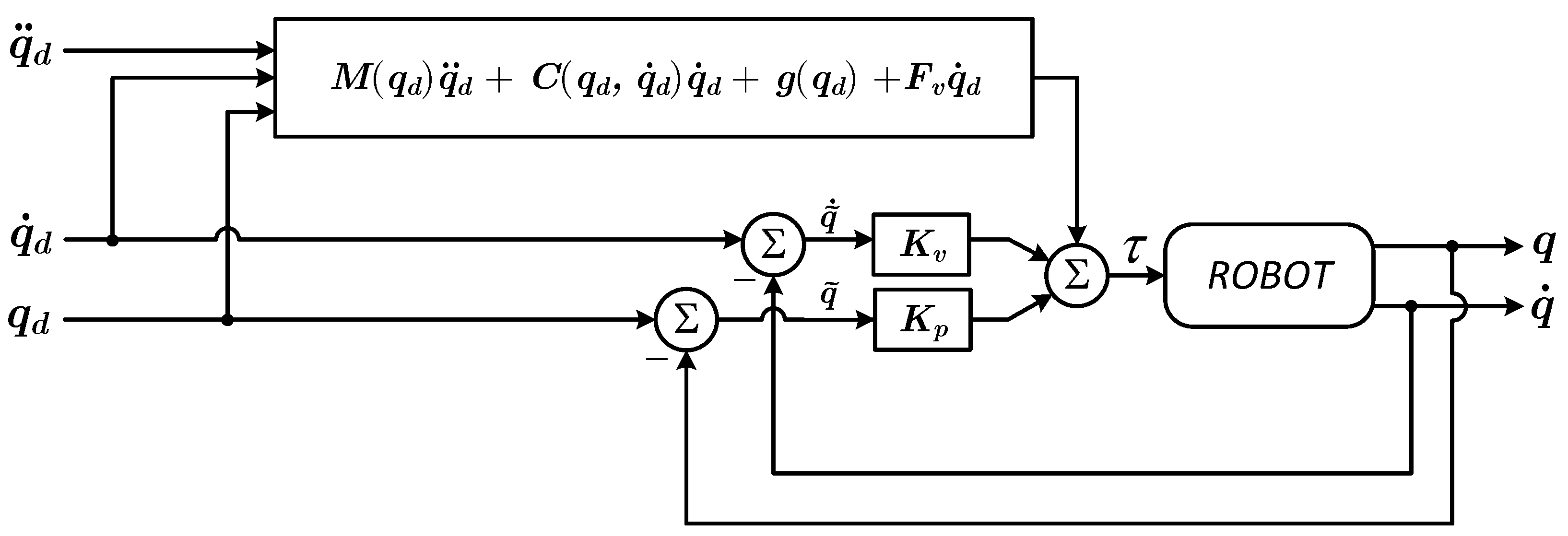
An important approach to the control of robot manipulators is model feedforward control. This simple strategy uses the inverse dynamics of a system, evaluated along reference signals, as the control law [9]. However, implementing this control strategy requires precise values of the robot model’s parameters. An enhancement to this strategy is represented by the PD model plus a feedforward control compensation scheme, which was analyzed and tested in [1]. They reported a stability analysis and experimental results for robot motion control using a PD plus feedforward controller, achieving performance comparable to the popular computed-torque control law. Recently, this approach has been extended to its fuzzy implementation in [10], where Global Uniform Asymptotic Stability (GUAS) for n-link serial robot manipulators has been formally proven, showing its good performance both in simulation and real-time experiments. To effectively utilize the excellent performance of PD control along with a feedforward controller, feedforward compensation is often implemented in an adaptive manner to address model uncertainties or disturbances. Artificial neural networks (ANNs), both feedforward-fixed and recurrent (adaptive) types, are the so-called battle horse of all current applications in Machine Learning for Robotic Control Systems, where they are extensively used to implement these types of systems [11]. In the work presented in [12], a fixed NN is applied to optimize the parameters of a Proportional–Integral–Derivative (PID) controller used in the tracking motion control of a Two-Degrees-of-Freedom (DOF) robotic arm. The NN yielded better results than those obtained via Genetic Algorithms or the cuckoo search algorithm. Performance comparisons were carried out with the PID parameter values obtained by the different optimization algorithms, demonstrating that their proposal showed the best results in terms of transient response and disturbance rejection. Adaptive neural networks have been extensively utilized in robot manipulators since the first successful approach introduced in [13]. This approach is illustrated in the work of [14], where an NN is used adaptively to model the desired dynamics of a robotic manipulator. This method is used in conjunction with a nonlinear PD controller to manage the motion trajectories of robot manipulators. Similarly, ref. [15] introduced a wavelet NN to control a deicing robot manipulator used on farm transmission lines. In this controller, the neural network was responsible for estimating the disturbances and unmodeled dynamics of the robot. A radial-basis adaptive NN was used to control a robotic arm with a unified objective bound in [16], showing satisfactory performance results. This unified objective bound includes all type of constraints related to various robotic manipulation tasks, such as transient performances, speed limits, and power consumption. However, the robot used only moved parallel to the horizontal plane such that no gravity vector was involved. Also, the control law used some discontinuous functions whose nature was not considered in the stability proof. In recent years, this approach has been expanded upon, as demonstrated by [17], who proposed an adaptive controller based on neural networks to address uncertainties and input saturation in robotic manipulators. In a study by [18], an adaptive NN controller was developed for n-serial robotic systems with time-varying state constraints. The researchers demonstrated the controller’s stability and achieved promising results in simulations. Additionally, in [19], the authors introduced a controller for an n-link constrained robotic arm, utilizing a radial-basis adaptive NN. They considered actuator dynamics, along with state and input constraints, as well as unknown time-varying delays, all at the same time. Time-varying barrier Lyapunov functions were employed, proving Semiglobally Uniformly Ultimately Bounded (SGUUB) closed-loop stability. Saturation functions and Lyapunov–Krasovskii functionals were used to eliminate the effects of actuator saturation and time delays. They validated their proposal via simulation studies. Also, in [20], a radial-basis NN is used in two parts to model and control a 6-DOF robotic arm. The article shows the whole procedure followed to construct the robot, along with the kinematic modeling and the controller design. The controller design uses a previous model of the robot estimated using a fixed radial-basis NN, and then an adaptive radial basis to control the trajectory tracking of their robot. The stability analysis is developed by applying Lyapunov theory. The controller performance is assessed by both simulation and experimental experiments, yielding excellent results with almost zero angular position errors and very minimal adaption time. In [21], a very similar control scheme to [14] is applied, combining feedback linearization (FDL) with a multilayer NN-based observer. Its stability is proven using Lyapunov’s second method. The authors carry out several simulations to test their proposed controller versus the FDL and PID approaches, considering both parametric uncertainties and strong external disturbances. An NN controller applied to the regulation of the position of a 3-DOF robot manipulator is described in [22]. In this work, a three-layer B-spline ANN is used to control the robotic arm using only the angular position errors at each joint as inputs to the NN. The paper includes both the development of the robot’s kinematic model and a comparative assessment of the new proposal versus a PID controller, with and without parameter deviations. The new controller shows acceptable angular position errors.
In the current work, using the new properties of sectorial fuzzy controllers (SFCs) presented in [10], which led to the discovery of strict Lyapunov functions that allowed us to conclude that GUAS should be utilized for sectorial fuzzy control (SFC) plus model feedforward compensation control of robot manipulators, a controller composed of an SFC in the feedback loop plus an adaptive NN in a feedforward array is proposed. This type of control proposal compensates for disturbances and parameter deviation, guaranteeing global uniform asymptotic motion trajectory tracking for robot manipulators of n-link at the same time. The adaptive NN is made up of three actual layers that require the calculation of two independent sets of weights, which is an initial step to implement this adaptive NN as a deep NN composed of a larger number of layers, as shown in [23]. Furthermore, formal stability analysis through Lyapunov functions and a LaSalle–Yoshizawa corollary for systems with discontinuities [24], which were not used in previous approaches, demonstrate that the proposed controller leads to global uniform convergence of position and velocity errors to zero, keeping all of its signals bounded. To the best of the authors’ knowledge, this proposed controller is the first motion trajectory controller for robot manipulators based on an SFC for a feedback loop with adaptive feedforward NN compensation that does not need knowledge of robot dynamics to achieve the control objective. Finally, intensive real-time experimental tests are carried out and compared with the angular position error performance achieved by two previously published motion controllers, where, in general, the best performance is achieved by the proposed SFC with an adaptive feedforward NN compensation controller.
The remainder of this paper is structured as follows: Section 2 presents a review of robot dynamics focused on its useful properties for stability analysis, along with a brief introduction to ANNs for modeling approximation, and the PD control plus feedforward compensation that our new proposal improves. 
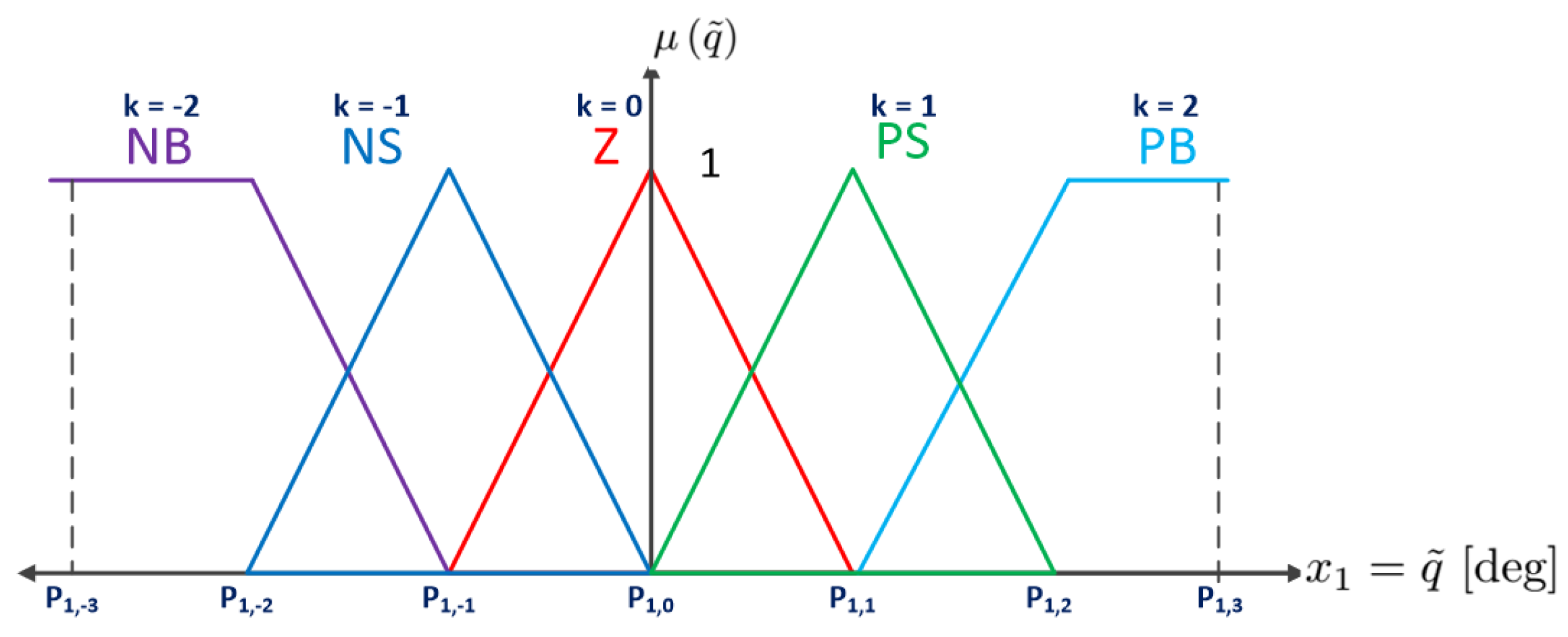
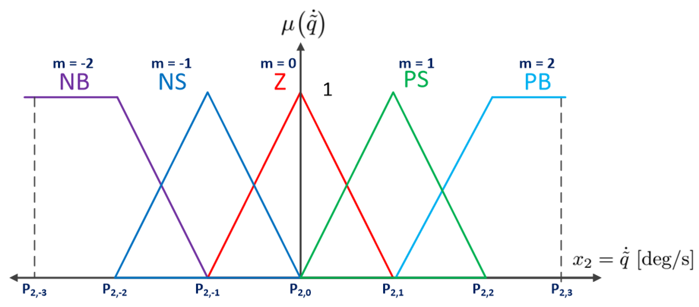
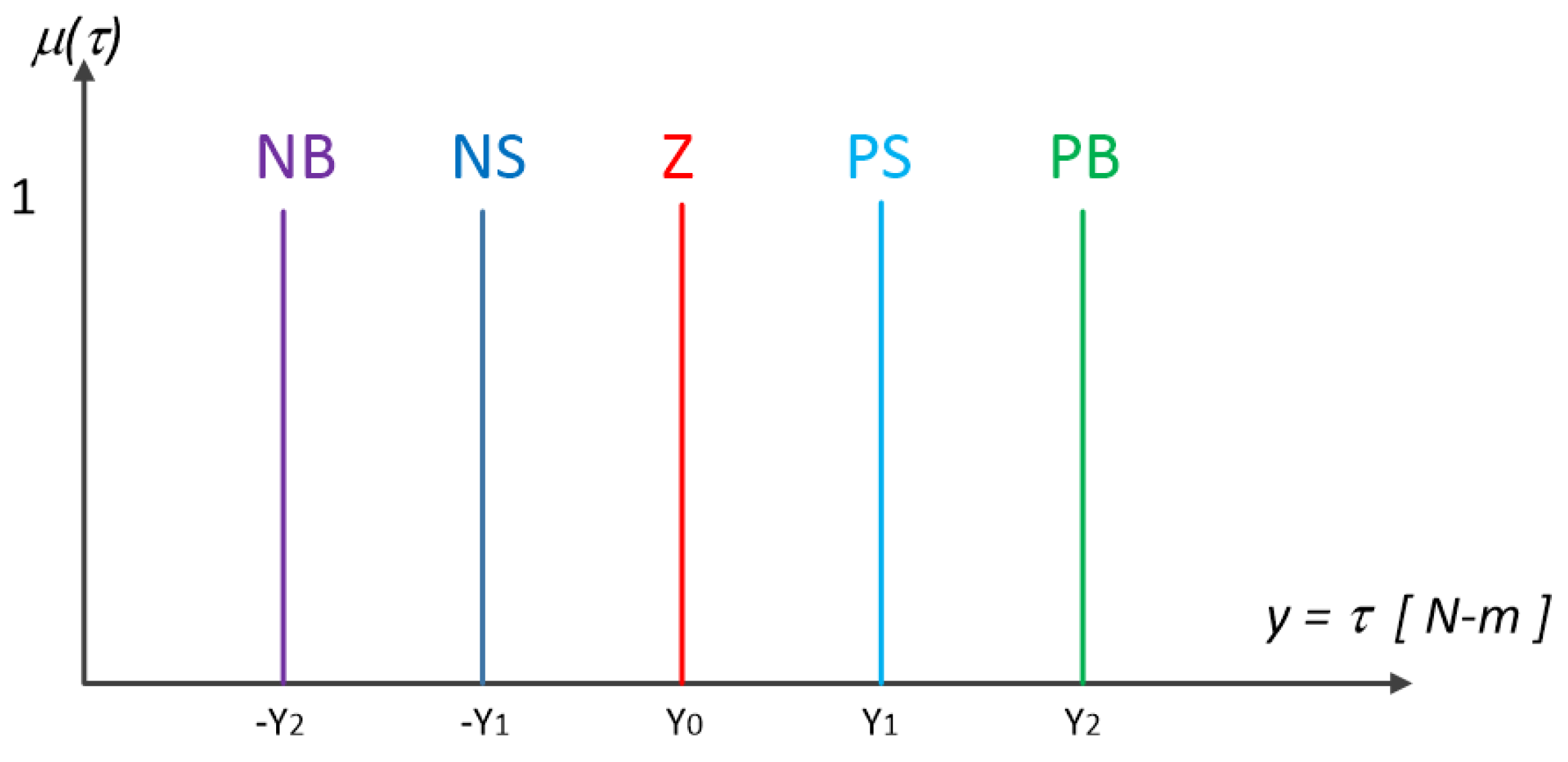
Section 3 presents the SFC, listing its main properties used for stability analysis. Section 4 introduces our new approach, the sectorial fuzzy controller with Adaptive NN compensation, its control law, and the adaptive dynamics for the NN weights. A stability analysis of the closed-loop error dynamics of our new control approach, applying a corollary of the LaSalle–Yoshizawa theorem for nonsmooth systems and Lyapunov stability theory, is presented in depth in Section 5. 
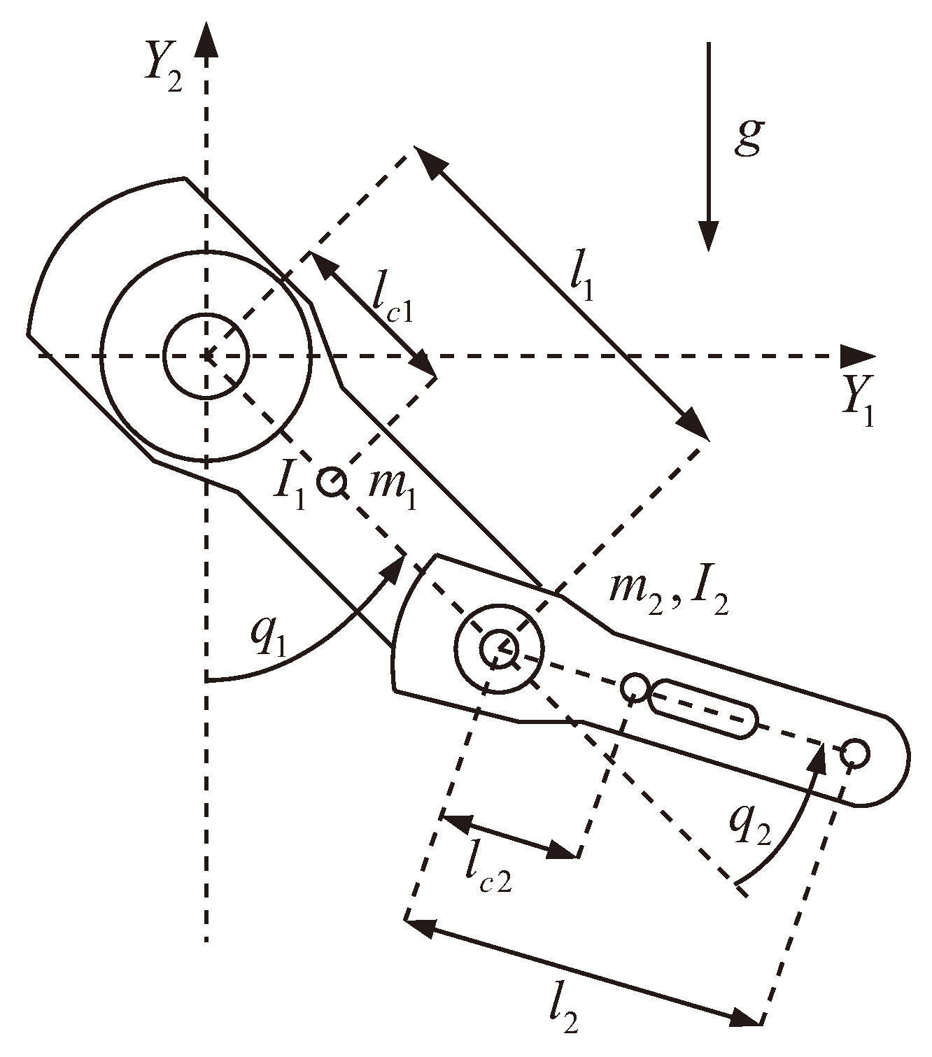
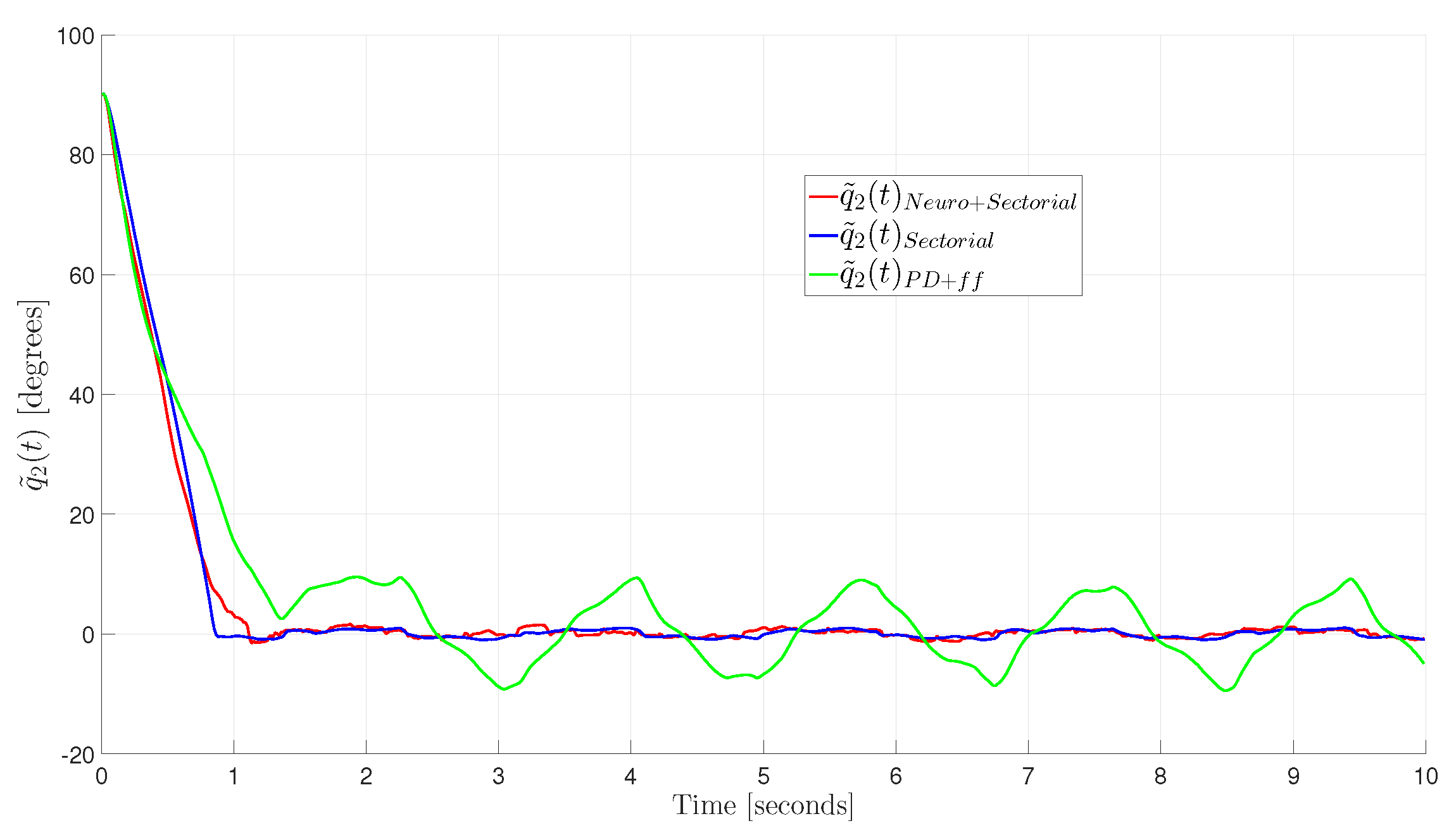
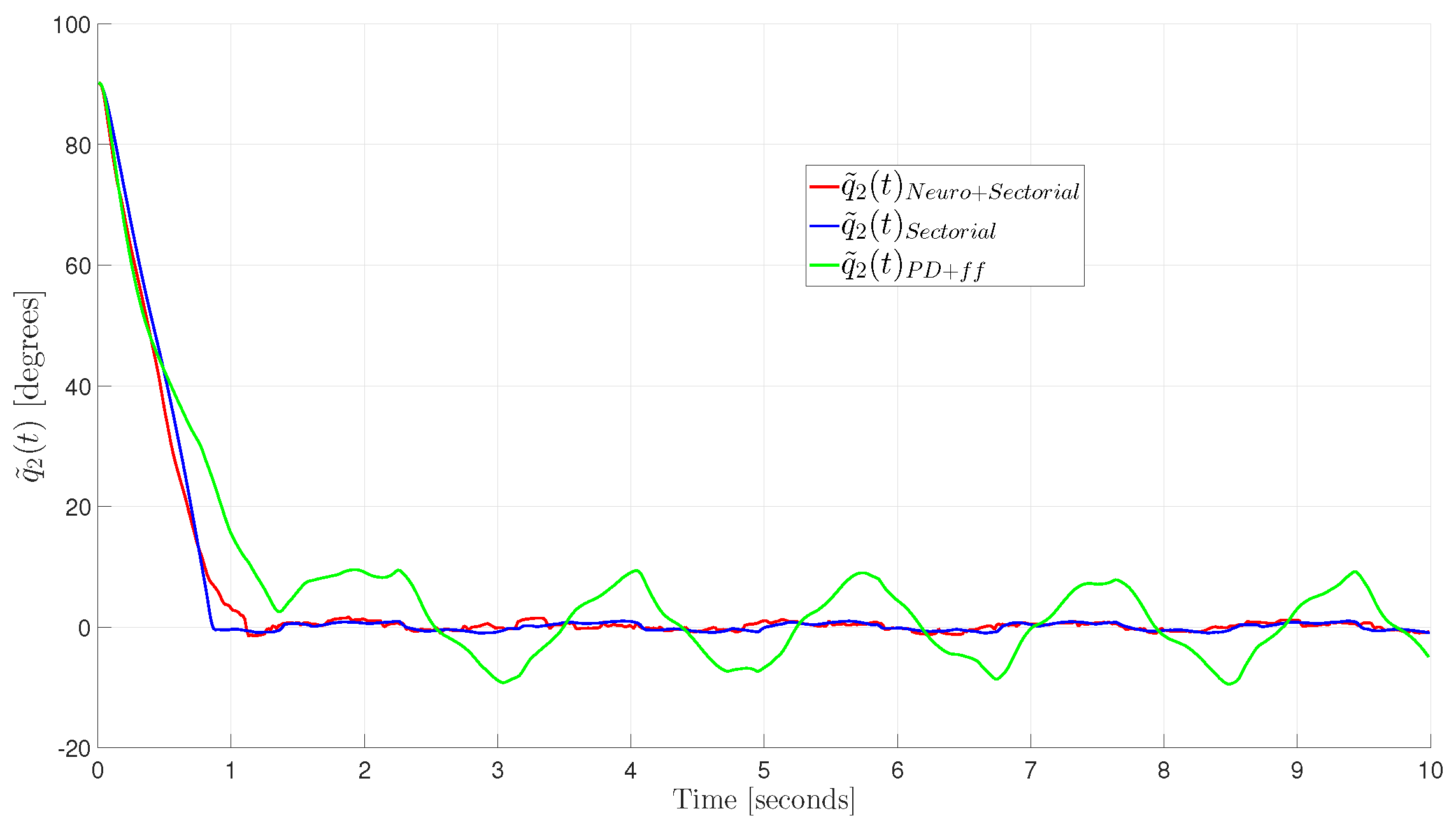
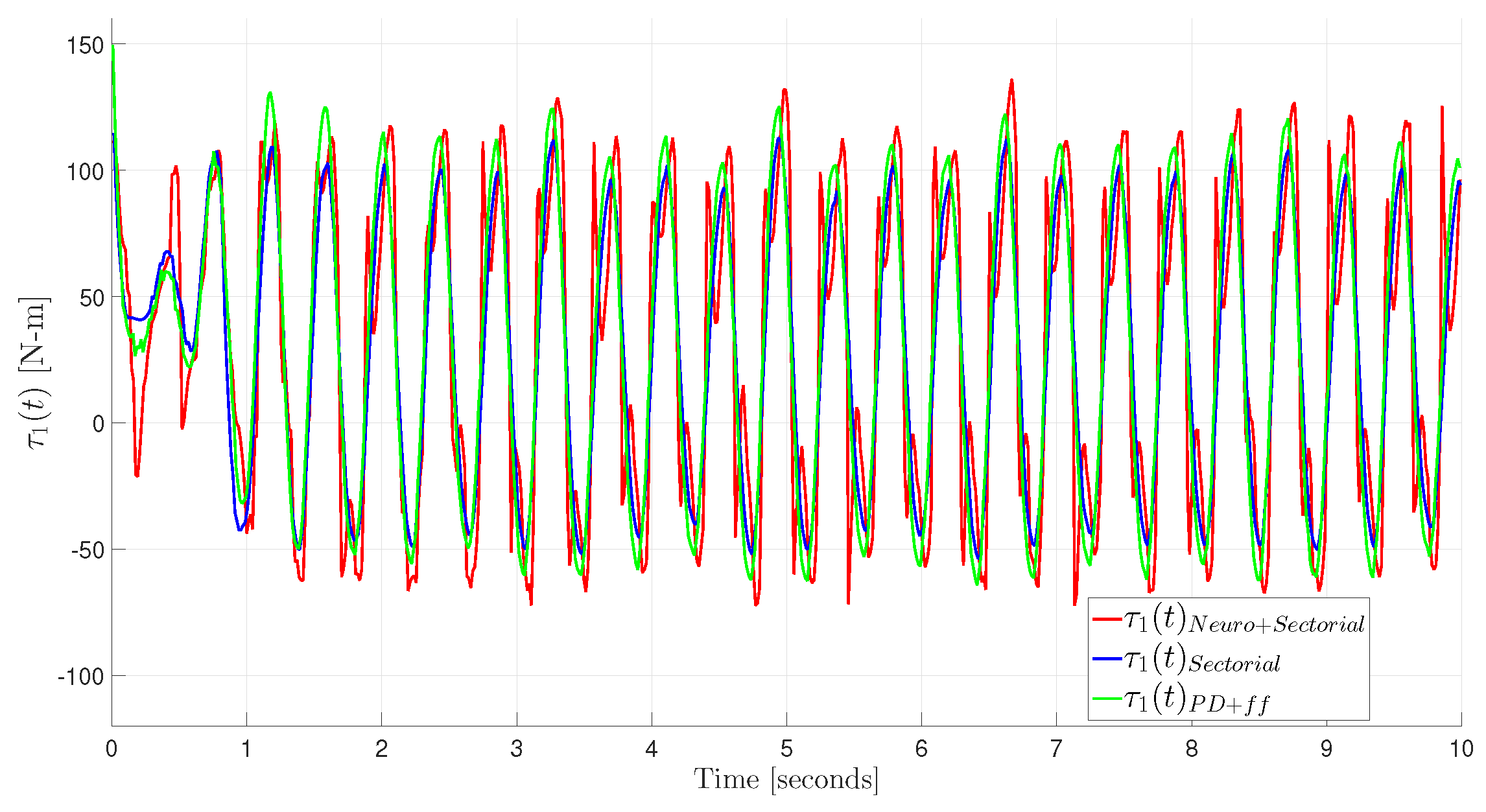
Section 6 shows the main characteristics of the 2-DOF robot that is used as the plant for all the controllers, and includes all the design information, numerical simulation information, and real-time experiments, as well as a performance comparison of our new proposed controller versus the other two previously published controllers. In Section 7, we present the main conclusions obtained from the comparative analysis of the simulation and real-time implementation of our proposal with respect to previous approaches.

2. Mathematical Preliminaries

2.1. Robotic Manipulator Dynamics

The dynamics of a serial n-link robot can be summarized by the Euler–Lagrange formulation [25,26] as follows:
M q q ¨ + C q , q ˙ q ˙ + g q + f q ˙ = τ + η
where M ( q ) is the n × n symmetric positive-definite inertia matrix; C ( q   q ˙ ) q ˙ is the n × 1 vector of centrifugal and Coriolis torques; g ( q ) is the vector of gravitational torques; η is the n-vector of uncertainties, which includes external disturbances and all uncertainties in the parameters and non-modeled dynamics in the robot manipulator; and f ( q ˙ ) is the n × 1 vector of friction torques. If a static model is assumed, friction is to be modeled by a vector f ( q ˙ ) R n that depends only on the joint velocity q ˙ and combines both viscous and Coulomb frictions such that it is defined as
f ( q ˙ ) = F v q ˙ + F C sgn ( q ˙ )
where both F v and F C are n × n diagonal positive-definite matrices, and their diagonal elements are the viscous friction parameters and the Coulomb friction parameters, respectively. Finally, sgn ( q ˙ ) is the vector sign function [1].
The dynamics of the n-link robot manipulator modeled by (1) has the following properties, which hold for robotic manipulators with only rigid-link revolving joints [1].
Property 1. 
The inertia matrix M q is both positive-definite and symmetric, such that
λ min { M } q 2 q T M ( q ) q λ max { M } q 2
where λ min { M } = inf q λ min { M ( q ) } , and λ max { M } is sup q λ max { M ( q ) } .
Property 2. 
The vector C ( q , x ) y can be upper bounded as
C ( q , x ) y k C 1 x y , q , x , y R n ; k C 1 > 0 .
Property 3. 
If the centrifugal and Coriolis torque matrices C ( q , q ˙ ) q ˙ are assumed to be obtained using Christoffel symbols of the first kind, then we have
q T M ˙ 2 C ( q , q ˙ ) q = 0 q , q ˙
and
M ˙ = C ( q , q ˙ ) + C ( q , q ˙ ) T .
Property 4. 
The residual dynamics, h ( q ˜ , q ˜ ˙ ) , ref. [27], is defined as
h ( q ˜ , q ˜ ˙ ) = M ( q d ) M ( q ) q ¨ d + g ( q d ) g ( q ) + C ( q d , q ˙ d ) C ( q , q ˙ ) q ˙ d
where q d is the desired angular joint position, assumed to be bounded, and at least three times differentiable with bounded derivatives for all t 0 . In addition,
q ˜ = q d q
is the angular joint position error.
The residual dynamics (7) has the property defined in (9) and satisfies the inequality (10) [1,10]
h ( 0 , 0 ) = 0 ,
and
h ( q ˜ , q ˜ ˙ ) k h 1 q ˜ ˙ + k h 2 tanh ( q ˜ ) ,
where k h 1 and k h 2 are sufficiently large strictly positive constants that depend on the robot model parameters.

2.2. Artificial Neural Networks

The Universal Approximation Theorem states that ANNs with one hidden layer can approximate any smooth continuous function within a given range that defines a compact domain [28,29]. Therefore, a multilayer ANN with a single hidden layer and output weights can also be used to learn the desired dynamics of a robot manipulator uniformly over a given compact domain, as is exemplified in [14]. This approximation is achieved by adjusting the ANN’s synaptic weights such that the error function between its output and the output of the function to be approximated (the desired robot dynamics, in this case) is minimized, as defined in (11):
f ( x ) = W T σ V T x + ϵ , x R N + 1
where f ( x ) R L is the function to be approximated by the ANN, x R N + 1 is the vector of input signals to the ANN, V R ( N + 1 ) × L is the optimal matrix of input weights, W R L × N + 1 is the optimal matrix of output weights, L is the number of neurons in the hidden layer, σ ( · ) R L is the activation function in the hidden layer, and ϵ R L is the approximation error, where
ϵ i E
holds i = 1 , 2 , , n , with E > 0 .
Since multilayered ANNs are nonlinear in their weights V due to their activation function, σ , a Taylor series can be applied to approximate it such that upon expanding σ at V ^ , which is the estimate of the optimal input weights V, we have
σ V T x = σ V ^ T x + σ V ^ T x V T x V ^ T x + 1 2 σ V ^ T x V T x V ^ T x 2 +
where σ V ^ T x is the Jacobian of σ V ^ T x ,
σ V ^ T x = σ ( x ) x ; x = V ^ T x d
We define the weight estimation errors V ˜ and W ˜ for both V and W , respectively, as
V ˜ = V V ^
W ˜ = W W ^
and the higher order terms as O V ˜ T x :
O V ˜ T x = 1 2 σ V ^ T x V ˜ T x 2 +
We can rewrite (13) as follows:
σ V T x = σ V ^ T x + σ V ^ T x V ˜ + O V ˜ T x

2.3. PD Control Plus Feedforward Controller

The original control proposal used for the trajectory control of robotic manipulators that we are trying to improve via a fuzzy controller and an ANN is the PD control plus feedforward controller. A block diagram of this control structure is shown in Figure 1.
The PD control plus feedforward controller analyzed in [1] is defined as
τ = K p q ˜ + K v q ˜ ˙ + M ( q d ) q ¨ d + C ( q d , q ˙ d ) q ˙ d + g ( q d ) + F v q ˙ d
where K p , K v R n × n are symmetric positive-definite matrices, called gains of position and velocity, respectively.

3. Sectorial Fuzzy Controller

An SFC Φ ( · , · ) [3] is a special type of fuzzy controller with two inputs and only one output, which form a nonlinear input–output static fuzzy mapping. Φ ( q ˜ , q ˜ ˙ ) [3,5] is an n × 1 vector whose elements ϕ i q ˜ i , q ˜ ˙ i , with i = 1 , 2 , 3 , , n , are the real input–output mappings of the SFC,
Φ q ˜ , q ˜ ˙ = ϕ 1 q ˜ 1 , q ˜ ˙ 1 ϕ 2 q ˜ 2 , q ˜ ˙ 2 ϕ n q ˜ n , q ˜ ˙ n
An SFC has useful sectorial properties that enable the analysis of its stability. These properties have been already proven in [3,5], and are listed below:
  • Property 1: ϕ ( 0 , 0 ) = 0 .
  • Property 2: ϕ i q ˜ i , q ˜ ˙ i = ϕ i q ˜ i , q ˜ ˙ i .
  • Property 3: there exists ζ i , ρ i > 0 , such that
    0 < q ˜ i ϕ i q ˜ i , q ˜ ˙ i ϕ i 0 , q ˜ ˙ i ρ i q ˜ i 2
    0 < q ˜ ˙ i ϕ i q ˜ i , q ˜ ˙ i ϕ i q ˜ i , 0 ζ i q ˜ ˙ i 2
  • Property 4: ϕ i q ˜ i , 0 = 0 q ˜ i = 0 .
  • Property 5: ϕ i q ˜ i , q ˜ ˙ i δ : = max l 1 , l 2 y ¯ l 1 , l 2 .
  • Property 6: y ¯ k , 0 ϕ i q ˜ i , 0 y ¯ k + 1 , 0 ; for i = 1 , 2 , 3 , , n , where y ¯ l 1 , l 2 , y ¯ k , 0 , y ¯ k + 1 , 0 define the centers of the corresponding output membership functions (MFs) that must be assigned by the control designer. Through the definition of the MFs, a piece-wise transient response can be given to the controlled system [30].
New properties were found and used in [10]
  • Property 7:
    ϕ i ( q ˜ i , q ˜ ˙ i ) ϕ i ( 0 , q ˜ ˙ i ) α i tanh ( q ˜ i )
    with α i defined as
    α i = φ i | min M < m < M { y ¯ i 1 , m y ¯ i 0 , m , y ¯ i 1 , m + 1 y ¯ i 0 , m + 1 , y ¯ i 0 , m y ¯ i 1 , m , y ¯ i 0 , m + 1 y ¯ i 1 , m + 1 } |
    where M is the maximum value of the partitions considered within the domain of discourse of q ˜ i in this case, and φ i > 0 is the upper bound of the derivative | μ i 1 0 ( q ˜ i ) | of the MF μ i 1 0 ( q ˜ i ) .
    | μ 1 0 ( q ˜ i ) | φ i
  • Property 8: given ζ i > 0 ,
    ϕ i 0 , q ˜ ˙ i ζ i q ˜ ˙ i .
An SFC will have the properties listed before in [10], “if it is designed using the following guidelines: Define a fuzzy system with one output computed as the fuzzy relationship of two inputs. Establish an odd number of input and output fuzzy sets covering the entire span of the fuzzified inputs considered, with all MFs symmetric with respect to zero. The MFs of adjacent input fuzzy sets must be defined to have complementary membership values for every crisp value. The definitions of fuzzy sets for the input MF are recommended to be convex in the sense given by [3]; therefore, around zero, only functions with one isolated maximum (like triangular MFs) can be used, where no trapezoidal or similar MFs are allowed. The consequents of the fuzzy rules table increase, logically speaking, from left to right, and from top to bottom, with a zero output when both inputs are zero. Due to the condition that must be met for Property 7 to exist, that is, ϕ i ( q ˜ i , q ˜ ˙ i ) ϕ i ( 0 , q ˜ ˙ i ) 0 , no column or row adjacent to a null input column or row, respectively, can have the same consequent. The output is computed by using the center average fuzzifier, applying the product inference method, and center average defuzzifier”, which will turn the output computing into a convex combination of its inputs as, demonstrated previously in [5,10,31].
From the properties defined for an SFC, we can develop the following useful relationships, which will be applied in the stability analysis of our proposed control scheme in Section 5:
By extending (25) to the vector-matrix case, we can rewrite
Φ 0 , q ˜ ˙ λ max { Z } q ˜ ˙
where Z = diag { ζ i } for i = 1 , 2 , n .
From Property 9, we can express (22) using the following general expression
Φ ( q ˜ , q ˜ ˙ ) Φ ( 0 , q ˜ ˙ ) λ min { A } tanh ( q ˜ )
with A = diag ( α i ) .
And from (20) in Property 3, it can be reinterpreted as
sign Φ ( q ˜ i , q ˜ ˙ i ) Φ ( 0 , q ˜ ˙ i ) = sign ( q ˜ i )
Also, considering that sign ( q ˜ i ) = sign tanh ( q ˜ i ) , (20) can be rewritten in vector notation as
tanh ( q ˜ ) T Φ ( q ˜ , q ˜ ˙ ) Φ ( 0 , q ˜ ˙ ) 0
Applying (22) to (29), we have
tanh ( q ˜ ) T Φ ( q ˜ , q ˜ ˙ ) Φ ( 0 , q ˜ ˙ ) tanh ( q ˜ ) T A tanh ( q ˜ ) tanh ( q ˜ ) T A tanh ( q ˜ ) λ min { A } tanh ( q ˜ ) 2 λ min { A } tanh ( q ˜ ) 2 > 0 q ˜ 0 R n
Finally, if we substitute q ˜ ˙ i = 0 in (22), it yields
ϕ i ( q ˜ i , 0 ) α i tanh ( q ˜ i )
which, in matrix expression, can be written as
Φ ( q ˜ , 0 ) λ min { A } tanh ( q ˜ ) .

4. Sectorial Fuzzy Controller with Adaptive Neural Network Compensation

A block diagram of our proposal is shown in Figure 2.
And its control law is given in (33):
τ = W ^ T σ V ^ T x d + Φ q ˜ , q ˜ ˙ + Δ sign ( r )
where
x d = q d T q ˙ d T q ¨ d T 1 T R N + 1
is the vector of input signals to the NN, consisting of the desired trajectories for the n joints of the robot, their two first derivatives (desired angular velocities and angular accelerations; therefore, N = 3 n ), and a normalized bias; Δ R n × n is a designed positive-definite matrix; L is the number of neurons to be applied; V ^ R N + 1 × L is the matrix of estimated input weights; and W ^ R L × n is the matrix of estimated output weights, where its update laws are defined in (35) and (36), respectively:
V ^ ˙ = R x d r T W ^ T σ ^
W ^ ˙ = F σ ^ σ ^ V ^ T x d r T
R R ( N + 1 ) × ( N + 1 ) , F R L × L are positive-definite matrices, σ ^ = σ V ^ T x d , and σ ^ is the Jacobian of σ ^ , as defined previously in (14). In addition,
r = q ˜ ˙ + γ tanh ( q ˜ )
where γ is a positive scalar.
Also, assuming that q d , q ˙ d , and q ¨ d are all bounded, the vector of input signals to the NN are also bounded:
x d < k x d ; with k x d > 0

5. Stability Analysis of SFC with Adaptive NN Compensation

5.1. LaSalle–Yoshizawa Corollary for Nonsmooth Systems

Since our control law (33) uses the sign function, sign ( · ) , which is discontinuous at the origin, this creates a differential equation with a right-hand side discontinuity (discontinuous on x and continuous on t) in the closed-loop error dynamics (54), which is the main equation where the stability of our control proposal will be proven. If the differential equation defining any system includes a right-hand-side discontinuity, its solution in the classical sense cannot be guaranteed; neither of these differential equations is locally Lipschitz. Several approaches to overcome the aforementioned problem have been proposed, of which Filippov solutions are the most formally accepted. Filippov generalizes the concept of a differential equation to a differential inclusion (set of differential equations) and allows us to formalize the stability analysis for nonsmooth right-hand-side differential equations. A typical Lyapunov stability analysis that uses smooth Lyapunov functions cannot be used to prove the stability of discontinuous systems. The latter naturally leads to the need to use a generalized Lyapunov analysis for nonsmooth systems. Therefore, we have included, with the aim of this manuscript being self-contained, the second corollary of this theorem developed in [24], which extends the stability analysis capacities of the LaSalle–Yoshizawa theorem. It adapts the LaSalle–Yoshizawa Theorem to systems where the time derivatives of the system states are not locally Lipschitz, applying Filippov solutions for nonautonomous nonlinear systems with right-hand-side discontinuities utilizing Lipschitz-continuous and regular Lyapunov functions whose time derivatives (in the sense of Filippov) can be upper bounded by negative semi-definite functions to prove stability. This corollary also uses and extends the applicability of Barbalat’s Lemma to prove stability.
Corollary 1 
([24]). For the system
x ˙ = f ( x ( t ) , t )
where x ( t ) D R n is the state vector, suppose f : D × [ 0 , ) R n is Lebesgue-measurable and essentially locally bounded, uniformly in t, and let D be an open and connected set containing x = 0 , and U : D × [ 0 , ) R be locally Lipschitz and regular such that
G 1 ( x ) U ( x , t ) G 2 ( x ) ,
U ˜ ˙ ( x , t ) G 3 ( x )
t 0 , x D where G 1 ( x ) and G 2 ( x ) are continuous positive-definite functions, and G 3 ( x ) is a continuous positive semi-definite function on D . Choose r > 0 and c > 0 such that B r D and c < min x = r G 1 ( x ) . Then, all Filippov solutions of (39) such that x ( t 0 ) { x B r | G 2 ( x ) c } are bounded and satisfy
G 3 x ( t ) 0 a s t
In this case, x ( t ) is assumed to be a Filippov solution of (39), and U ˜ ˙ ( x , t ) is the time derivative of the regular function U ( x , t ) , obtained via Clarke’s generalized gradient, computed as
U ˜ ˙ ( x , t ) = ξ U ( x , t ) ξ T K [ f ] ( x ( t ) , t ) 1
where K [ f ] ( x ( t ) , t ) is an upper semi-continuous, nonempty, compact and convex valued map on D defined as
K [ f ] ( x ( t ) , t ) = δ > 0 μ ( M = 0 ) c o ¯ f B x ( t ) , δ M , t
with μ ( M = 0 ) being the intersection over sets M of Lebesgue measure zero, c o ¯ being the convex closure, and
B x ( t ) , δ = { υ R n | x ( t ) υ < δ }
An arbitrary set of measure zero in B x ( t ) , δ will be excluded from the evaluation of K [ f ] ( x ( t ) , t ) , so that the result is the same for two vector fields that differ on a set of Lebesgue measure zero, according to Filippov theory [32].
Thus, the Lyapunov function, U ( x , t ) , to be used in order to apply this corollary of the LaSalle–Yoshizawa Theorem, must be both decrescent and radially unbounded, as stated in (40); and its time derivative must be negative semidefinite as in (41).

5.2. Closed-Loop Error Dynamics

The closed-loop equivalent of the system represented in the diagram shown in Figure 2 is obtained by first considering the Coulomb friction terms as part of the uncertainties in the robot dynamics model defined in (1); since they are unknown, we have
τ = M ( q ) q ¨ + C ( q , q ˙ ) q ˙ + g ( q ) + F v q ˙
We define the desired torque function, τ d from (46) as follows:
τ d = M ( q d ) q ¨ d + C ( q d , q ˙ d ) q ˙ d + g ( q d ) + F v q ˙ d
Subtracting (46) from (47), we have
τ d τ = M ( q d ) q ¨ d + C ( q d , q ˙ d ) q ˙ d + g ( q d ) + F v q ˙ d M ( q ) q ¨ C ( q , q ˙ ) q ˙ g ( q ) F v q ˙
which leads to
τ d τ = M ( q ) q ˜ ¨ + C ( q , q ˙ ) q ˜ ˙ + F v q ˜ ˙ + h ( q ˜ , q ˜ ˙ ) ,
where the residual dynamics, h ( q ˜ , q ˜ ˙ ) was used as defined in (7).
Now, we approximate the desired torque, τ d , in (47) by means of an NN:
τ d = W T σ V T x d + ϵ
with x d defined as in (34).
Substituting the control law (33) and the approximation of τ d (49) in (48) yields
M ( q ) q ˜ ¨ + C ( q , q ˙ ) q ˜ ˙ + F v q ˜ ˙ + h ( q ˜ , q ˜ ˙ ) = W T σ V T x d W ^ T σ V ^ T x d + ϵ Φ q ˜ , q ˜ ˙ Δ sign ( r )
We apply Taylor series expansion to the activation function, σ , on (50), and simplify
M ( q ) q ˜ ¨ = C ( q , q ˙ ) q ˜ ˙ F v q ˜ ˙ h ( q ˜ , q ˜ ˙ ) + W ˜ T σ ^ W ˜ T σ ^ V ^ T x d + W ^ T σ ^ V ˜ T x d + ω ( t ) Φ q ˜ , q ˜ ˙ Δ sign ( r )
where ω ( t ) is defined as
ω ( t ) = W ˜ T σ ^ V T x d + W T O V ˜ T x d + ϵ
If the activation function being used is analytical, ω ( t ) is assumed to be bounded [14]:
ω ( t ) k ω
Including both the output and input weight update dynamics, V and W , given in (36) and (35), respectively, and expressing them in terms of V ˜ , W ˜ , the whole closed-loop errors dynamics can be expressed in matrix notation as
d d t q ˜ q ˜ ˙ V ˜ W ˜ = q ˜ ˙ M ( q ) 1 [ C ( q , q ˙ ) q ˜ ˙ F v q ˜ ˙ h ( q ˜ , q ˜ ˙ ) + W ˜ T σ ^ W ˜ T σ ^ V ^ T x d + W ˜ T σ ^ V ˜ T x d + ω ( t ) Φ q ˜ , q ˜ ˙ Δ sign ( r ) ] R x d r T W T W ˜ T σ ^ F σ ^ σ ^ V T x d + σ ^ V ˜ T x d r T

5.3. Lyapunov Function Candidate

The stability analysis for the closed-loop system is formalized in the following paragraphs. The proposed Lyapunov function candidate (LFC) is
U ( q ˜ , q ˜ ˙ , V ˜ , W ˜ , t ) = 1 2 q ˜ ˙ T M ( q ) q ˜ ˙ + i = 1 n 0 q ˜ i ϕ ( ξ i , 0 ) d ξ i + 1 2 tr ( V ˜ T R 1 V ˜ ) + 1 2 tr ( W ˜ T F 1 W ˜ ) + γ tanh ( q ˜ ) T M ( q ) q ˜ ˙ .
To be able to apply the corollary presented in (41), our LFC must be proven to be both radially unbounded and decrescent. To work out the radially unbounded property, first, we focus on the fuzzy related term of (55), and by applying Property 7 of an SFC given in (22), the next inequalities can be developed:
i = 1 n 0 q ˜ i ϕ ( ξ i , 0 ) d ξ i i = 1 n α i 0 q ˜ i tanh ( ξ i ) d ξ i
= i = 1 n α i | ln cos h ( q ˜ i ) | i = 1 n α i β i | tanh ( q ˜ i ) | 2
λ min { AB } tanh ( q ˜ ) 2 .
In (57), we use ln { cosh ( q ˜ i ) } β i tanh ( q ˜ i ) 2 , with 0 β i 1 2 , and B = diag { β i } , for i = 1 , 2 , n .
Upon partitioning the integral term in (55) into two halves, using the first part of the result of (57) in the first half of this partition and the result of (58) in the other one, and applying the bounds defined in Property A of the robot dynamic model (3), we have
U ( · ) 1 2 λ min { M } q ˜ ˙ 2 + 1 2 ( i = 1 n α i | ln cos h ( q ˜ i ) | + λ min { A B } tanh ( q ˜ ) 2 ) + 1 2 tr ( V ˜ T R 1 V ˜ ) + 1 2 tr ( W ˜ T F 1 W ˜ ) γ λ max { M } tanh ( q ˜ ) q ˜ ˙ .
We organize (59)’s quadratic form,
U ( · ) 1 2 ( tanh ( q ˜ ) q ˜ ˙ T q 1 tanh ( q ˜ ) q ˜ ˙ + i = 1 n α i | ln cos h ( q ˜ i ) | + tr ( V ˜ T R 1 V ˜ ) + tr ( W ˜ T F 1 W ˜ ) )
with
q 1 = λ min { A B } γ λ max { M } γ λ max { M } λ min { M }
where q 1 is positive-definite if, first, λ min { A B } > 0 , which is already fulfilled, since A , B > 0 , and second,
det q 1 = λ min { M } λ min { A B } γ 2 λ max { M } 2 > 0
holds. Calculating γ from (62), we have
0 < γ < λ min { M } λ min { A B } λ max { M }
The existence of this value of γ ensures that our proposed LFC, given in (55), is both globally positive-definite and radially unbounded. To prove that U ( q ˜ , q ˜ ˙ , V ˜ , W ˜ , t ) is also a decrescent function, we now use Property 3 of an SFC given in (20) with q ˜ ˙ i = 0 , with the integral term of (55):
0 q ˜ i ϕ ( ξ i , 0 ) d ξ i ρ i 0 q ˜ i ξ i d ξ i ρ i 2 q ˜ i 2
Applying this result to (55), the upper bound of the LFC is given by
U ( · ) 1 2 [ λ max { M } q ˜ ˙ 2 + λ max { R o } q ˜ 2 + tr V ˜ T R 1 V ˜ + tr W ˜ T F 1 W ˜ ] + γ λ max { M } q ˜ ˙
with R o = diag { ρ i } , i = 1 n .
Thus, our proposed LFC, given in (55), is a globally positive-definite radially unbounded decrescent function that can be used with the corollary of the LaSalle–Yoshizawa stability theorem as a valid Lyapunov Function (LF) in the stability analysis of our control scheme proposal.

5.4. Time Derivative of the Lyapunov Function

In order to apply the corollary for the LaSalle–Yoshizawa stability theorem, it is necessary to calculate the time derivative of the LF in the trajectories of the dynamics of the system given in (54). Since our LF is fully differentiable, the generalized Clarke gradient reduces to the standard gradient. Now, applying Leibniz’s rule to the integral term of (55), we have
U ˜ ˙ ( q ˜ , q ˜ ˙ , V ˜ , W ˜ , t ) q ˜ ˙ T M ( q ) q ˜ ¨ + 1 2 q ˜ ˙ T M ˙ ( q ) q ˜ ˙ + Φ ( q ˜ , 0 ) T q ˜ ˙ + tr V ˜ T R 1 V ˜ ˙ + tr W ˜ T F 1 W ˜ ˙ + γ [ sech 2 ( q ˜ ) q ˜ ˙ ] T M ( q ) q ˜ ˙ + γ tanh ( q ˜ ) T M ˙ ( q ) q ˜ ˙ + γ tanh ( q ˜ ) T M ( q ) q ˜ ¨
We substitute q ˜ ¨ from the closed-loop equation in (51), apply the properties of the robot model dynamics defined in (5) and (6), and simplify
U ˜ ˙ ( · ) q ˜ ˙ T Φ ( q ˜ , q ˜ ˙ ) Φ ( q ˜ , 0 ) ] q ˜ ˙ T F v q ˜ ˙ γ tanh ( q ˜ ) T F v q ˜ ˙ q ˜ ˙ T h ( q ˜ , q ˜ ˙ ) γ tanh ( q ˜ ) T h ( q ˜ , q ˜ ˙ ) + γ tanh ( q ˜ ) T C T ( q ˜ , q ˜ ˙ ) q ˜ ˙ + γ q ˜ ˙ T sech 2 ( q ˜ ) M ( q ) q ˜ ˙ γ tanh ( q ˜ ) T Φ ( q ˜ , q ˜ ˙ ) tr V ˜ T R 1 V ^ ˙ tr W ˜ T F 1 W ^ ˙ + r T W ˜ T σ ^ W ˜ T σ ^ V ^ T x d + W ^ T σ ^ V ˜ T x d + r T ω ( t ) Δ SIGN ( r )
with r defined as in (37), and
SIGN ( r ) = K [ sign ] ( r ) = SIGN ( r 1 ) SIGN ( r 2 ) SIGN ( r 3 ) SIGN ( r n )
where
SIGN ( r j ) = 1 ; r j > 0 [ 1   1 ] ; r j = 0 1 ; r j < 0
Using the properties between the matrix trace and the transposition to the multiplication of vectors, substituting the functions for V ^ ˙ T   and   W ^ ˙ T , defined in (35) and (36), respectively, yields
U ˜ ˙ ( · ) q ˜ ˙ T Φ ( q ˜ , q ˜ ˙ ) Φ ( q ˜ , 0 ) q ˜ ˙ T F v q ˜ ˙ γ tanh ( q ˜ ) T F v q ˜ ˙ q ˜ ˙ T h ( q ˜ , q ˜ ˙ ) γ tanh ( q ˜ ) T h ( q ˜ , q ˜ ˙ ) + γ tanh ( q ˜ ) T C T ( q , q ˙ ) q ˜ ˙ + γ q ˜ ˙ T sech 2 ( q ˜ ) M ( q ) q ˜ ˙ γ tanh ( q ˜ ) T Φ ( q ˜ , q ˜ ˙ ) + r T ω ( t ) Δ SIGN ( r )
For the last term in (53), by applying the Cauchy–Schwarz inequality, given that the norms r r 1 are equivalent, and also the bound for ω ( t ) given in (52), we have
r T ω ( t ) Δ SIGN ( r ) [ λ min { Δ } k ω ] j = 0 n | r j |
Applying the relationships defined in (4), (10), and (53), and the bounds in (26), (30), and (71), we have
U ˜ ˙ ( · ) q ˜ ˙ T Φ ( q ˜ , q ˜ ˙ ) Φ ( q ˜ , 0 ) ] γ λ min { A } k h 2 tanh ( q ˜ ) 2 + γ λ max { Z } + λ max { F v } + k h 2 γ + k h 1 + k C 1 q ˙ M tanh ( q ˜ ) q ˜ ˙ γ λ min { F v } k h 1 γ n k C 1 λ max { M } q ˜ ˙ 2 [ λ min { Δ } k ω ] j = 0 n | r j | .
Defining the terms
a = λ min { A } k h 2 , b = k h 2
c = λ max { Z } + λ max { F v } + k h 1 + k C 1 q ˙ M
d = λ min { F v } k h 1 , e = n k C 1 + λ max { M }
and substituting them in (72), we have
U ˜ ˙ ( · ) q ˜ ˙ T Φ ( q ˜ , q ˜ ˙ ) Φ ( q ˜ , 0 ) γ tanh ( q ˜ ) q ˜ ˙ T q 3 tanh ( q ˜ ) q ˜ ˙ [ λ min { Δ } k ω ] j = 0 n | r j |
with
q 3 = a b γ + c 2 b γ + c 2 d γ e
Since Property 3 of SFCs holds for the first term of (76),
λ min { Δ } k ω , Q 3 > 0 U ˙ ( · ) < 0 .
Thus, we can derive the following relationships
λ min { A } > k h 2 a > 0 λ min { F v } > γ ( n k C 1 + λ max { M } ) + k h 1 d γ e > 0 det Q 3 > 0
where
det Q 3 = a d γ e b γ + c 2 4 > 0 .
Obtaining λ min { A } from (73) and (78), we obtain:
λ min { A } > k h 2 + k h 2 + γ c 2 4 γ λ min { F v } γ n k C 1 λ max { M } k h 1 .
U ˜ ˙ ( · ) γ tanh ( q ˜ ) q ˜ ˙ T q 3 tanh ( q ˜ ) q ˜ ˙ G 3 ( · ) .
Since q 3 is positive-definite, the function G 3 ( · ) that must be found, according to the the LaSalle–Yoshizawa corollary for nonsmooth systems, is also positive-definite. Therefore, it is possible to state that the angular position and velocity errors globally converge to zero:
lim t q ˜ = 0 , lim t q ˜ ˙ = 0 .
Remark 1. 
The value of λ min { Δ } is determined during the experimental stage and is used as a tuning parameter. A gain that is smaller than necessary would theoretically result in input-to-state stability [33], which implies that a smaller-than-necessary gain would not make the system’s solutions grow unbounded under the proposed control action. This allows for appropriate implementation of the control law. Also, both input and output weights, V and W , must be initialized, and in most cases, the whole ANN will be pretrained off-line to learn the desired dynamics; therefore, W ˜ in t = t 0 will be very small. If W were initialized in zero, as is the case in many off-line training algorithms, the maximum value of the spectral norm of W ˜ would be the same as the upper bound of the whole robot norm.

6. Controller Design, Simulation, and Experimentation

To asses the performance of our new proposal, we implemented it on a 2-DOF robot manipulator in a comparative fashion versus two other controllers, the PD plus feedforward controller and the SFC plus feedforward controller, and its design is described in the following subsections along with a description of the robot used.

6.1. 2-DOF Robot Manipulator Description

All control schemes to be compared were implemented for a 2-DOF robot manipulator that operates only vertically, as shown in Figure 3 [1,10,34,35]. The robot manipulator is composed of two rigid links. Every joint is driven by high-torque brushless direct-drive servos with no gear reduction, which reduces backlash and significantly diminishes joint friction compared to using gear drives. The maximum torques that can be applied, according to the manufacturer, is 150 [N–m] for joint 1 and 15 [N–m] for joint 2. The values for all the mechanical parameters of this robot are given in Table 1.
The dynamical model of the robot manipulator shown in Figure 3 can be expressed as
M 11 ( q ) M 12 ( q ) M 21 ( q ) M 22 ( q ) M ( q ) q ¨ + C 11 ( q , q ˙ ) C 12 ( q , q ˙ ) C 21 ( q , q ˙ ) C 22 ( q , q ˙ ) C ( q , q ˙ ) q ˙ + g 1 ( q ) g 2 ( q ) g ( q ) + f v 1 0 0 f v 2 F v q ˙ = τ
with
M 11 ( q ) = m 1 l c 1 2 + m 2 [ l 1 2 + l c 2 2 + 2 l 1 l c 2 cos ( q 2 ) ] + I 1 + I 2 , M 12 ( q ) = m 2 [ l c 2 2 + l 1 l c 2 cos ( q 2 ) ] + I 2 , M 21 ( q ) = m 2 [ l c 2 2 + l 1 l c 2 cos ( q 2 ) ] + I 2 , M 22 ( q ) = m 2 l c 2 2 + I 2 , C 11 ( q , q ˙ ) = m 2 l 1 l c 2 sin ( q 2 ) q ˙ 2 , C 12 ( q , q ˙ ) = m 2 l 1 l c 2 sin ( q 2 ) [ q ˙ 1 + q ˙ 2 ] C 21 ( q , q ˙ ) = m 2 l 1 l c 2 sin ( q 2 ) q ˙ 1 , C 22 ( q , q ˙ ) = 0 , g 1 ( q ) = [ m 1 l c 1 + m 2 l 1 ] g sin ( q 1 ) + m 2 l c 2 g sin ( q 1 + q 2 ) , g 2 ( q ) = m 2 l c 2 g sin ( q 1 + q 2 ) ,
In this case, the Coulomb friction terms were neglected and will be considered as a disturbance within the robot model that the controllers to be tested must overcome.

6.2. PD Plus Feedforward Controller Design

For this controller, its gain matrices K p , K v R 2 × 2 were assigned the values
K p = 225 0 0 10 K v = 70 0 0 4
These values were proposed based on the minima defined in [34] so that the torques applied to joints 1 and 2 of the robot manipulator do not exceed their limit values of 150 N-m and 15 N-m, respectively.

6.3. Proposal of New Tracking Controller with Feedforward Compensation Based on SFC and Adaptive NN

For this controller, we used the design already carried out in our previous manuscript [10,35]; the second reference was only supported by experimental tests; in contrast, the current manuscript presents a formal stability analysis guaranteeing that position and velocity errors converge to zero and all signals are uniformly bounded. The MFs for each input of each joint and for the output were defined as shown in Figure 4, Figure 5, and Figure 6, respectively. The output MF was defined by singletons to expedite the complete output calculation in real time. In the definition of fuzzy sets, the acronyms used for each MF, for both inputs and the output, are as follows: NB = Negative Big; NS = Negative Small; Z = Zero; PS = Positive Small; and PB = Positive Big.
The fuzzy rules were defined as shown in Table 2 so that they followed the guidelines indicated in Section 3 to define an SFC.
The base values for the fuzzy sets were calculated using Genetic Algorithms (GAs), similar to those previously shown in [36]. The final support values for the fuzzy sets depicted in Figure 4, Figure 5 and Figure 6 are given in Table 3 for joint 1 and in Table 4 for joint 2.

6.4. SFC with Adaptive NN Compensation Controller Design

For this control scheme, we first used all MFs that were previously designed for the SFC plus feedforward controller, along with the fuzzy rules table and MFs for the outputs. For the adaptive NN compensation, N = 3 n = 3 ( 2 ) = 6 , with n = 2 , since the robot manipulator is composed of two links. We tried different activation functions, and finally selected σ ( x ) = tanh ( x ) because it was the one that performed the best. Also, we tested our controller in a simulation with different numbers of neurons, and set the number of neurons to be used to 20; therefore, L = 20 . The NN was first pre-trained in the simulation several times using the whole controller with the SFC block designed in the previous section until we obtained suitable values for the weights that avoided both start-up overshoots and surpassing the maximum allowed values for torques that can be applied to the two joints; in addition, they resulted in a fast response time and lower steady-state errors. The other design matrices and scalars that were part of the control law or adaptive dynamics of our proposed controller were given the following values:
α = 7.7 , γ = 0.4 , Δ = diag { 0.69 } , R = diag ( 2.6 ) , F = diag ( 2.2 )

6.5. Simulation of the Controllers

We used the model of the 2-DOF robot manipulator described in Section 6.1, including both viscous and Coulomb frictions. The desired angular position, angular velocity, and joint acceleration trajectories, q d ( t ) , q ˙ d ( t ) , and q ¨ d ( t ) , are given in the following equations, according to the values and functions proposed in [1], in order to achieve the maximum allowable performance for this specific robot manipulator:
q 1 d ( t ) = a 1 + b 1 ( 1 e d 1 t 3 ) + c 1 ( 1 e d 1 t 3 ) sin ( ω 1 t ) [ rad ] q 2 d ( t ) = a 2 + b 2 ( 1 e d 2 t 3 ) + c 2 ( 1 e d 2 t 3 ) sin ( ω 2 t ) [ rad ]
where a 1 = π / 2 [rad], b 1 = π / 4 [rad], c 1 = π / 18 [rad], d 1 = 2 , ω 1 = 15 [rad/s], a 2 = π / 2 [rad], b 2 = π / 3 [rad], c 2 = 25 π / 36 [rad], d 2 = 1.8 , and ω 2 = 3.5 [rad/s]. The desired angular velocities and accelerations were analytically computed by calculating the direct derivative of the desired angular positions.
All controllers were implemented and simulated in the Simulink software of MATLAB R2015a environment ® (MATLAB is a registered trademark of MathWorks, Inc., Natick, MA, USA). and their angular positions, angular position errors, and applied torques in each joint were obtained numerically and graphically. A comparison of the Root Mean Square (RMS) of every angular position error, computed using the function rms from Matlab for each joint, is shown in a comparative fashion for every controller tested in Table 5. All values are the RMS; the suffix “ss” represents steady-state values, calculated from 5 s to the end of the simulation time window of 10 s.
Both the SFC plus feedforward controller and the SFC plus adaptive NN compensation controllers show better position angular error performance than the original controller they are derived from, the PD plus feedforward controller. The SFC plus feedforward controller presents smaller values of angular position errors on both joints in comparison to the other controllers for the whole simulation, whereas the SFC plus adaptive NN compensation is the controller that has the smallest steady-state angular position errors thanks to the adaptive NN feedforward compensation. The SFC plus adaptive NN compensation has slightly larger total angular position errors than its SFC plus feedforward counterpart because the adaptive NN takes a moment to adapt, while the feedforward compensation in the second controller already has the complete model from the start.

6.6. Comparison of the Experimental Performance of the Controllers

All previously designed and simulated controllers were implemented on a PC-based real-time platform for real-time simulation and control of the 2-DOF robot manipulator (see Figure 7) in a real-time Microsoft Windows application called WinMechLab running on a old 800 MHz dual-core desktop personal computer. Both W ( t ) and V ( t ) were computed by integrating the weight update dynamics W ˙ ( t ) and V ˙ ( t ) defined in (35) and (36), respectively, through typical rectangular numeric integration. The sample period used was 2.5 ms (sampling frequency of 400 Hz). A MultiQ-PCI data acquisition board from Quanser Consulting, Inc, was used as the digital input/output hardware interface. The angular position error responses were obtained for each joint, as were the applied torques, as shown in Figure 8, Figure 9, Figure 10 and Figure 11.
In Table 6, a comparison of the position error RMS in each joint is shown for each controller. Again, all values are the RMS, obtained using the function rms in Matlab, and “ss” stands for steady-state values, which were computed from 5 s to the end of the time window of 10 s for the experiment.
Again, both the angular position errors and torques applied to joints 1 and 2 have smaller values for the SFC plus feedforward controller and the SFC plus adaptive NN compensation compared to the PD plus feedforward controller. In the experimental case, the SFC plus adaptive NN yielded larger errors in both joints for both the complete and the steady-state analyses compared to the SFC plus feedforward controller, since it was affected by the bit-resolution available in the real-time platform we had available to compute the values of the NN weights. In the simulation, we were using a 64-bit double real-number definition, while in the real-time implementation, only single 32-bit real number resolution was available.

7. Concluding Remarks

An SFC plus adaptive NN feedforward controller applied to the trajectory tracking control of robotic manipulators is presented along with a formal stability proof applying the LaSalle–Yoshizawa corollaries for nonsmooth systems. We successfully evaluated our new controller proposal both in simulation and in real-time experiments, comparing it with a previous approach (SFC plus feedforward compensation of the robot model) and the original classic scheme (PD plus feedforward compensation of the robot model). As a result of the stability analysis and real-time experiments, we can highlight that our new control proposal excludes the need for knowledge of the robotic manipulator model to achieve excellent results. And in the case of the real-time experimental implementation of SFC plus feedforward compensation, there was no need to retune any control parameters obtained via simulation, unlike classical PD plus feedforward compensation, which required several changes to its control parameters in order to obtain decent experimental performance results.

Author Contributions

Conceptualization, A.P.-L., V.S. and R.G.-H.; methodology, A.P.-L., V.S. and R.G.-H.; software, A.P.-L., R.G.-H. and J.V.-C.; validation, A.P.-L., V.S., R.G.-H., J.V.-C. and J.M.-V.; formal analysis, A.P.-L., V.S. and J.V.-C.; investigation, A.P.-L., V.S., R.G.-H., J.V.-C. and J.M.-V.; resources, V.S. and R.G.-H.; data curation, A.P.-L.; writing—original draft preparation, A.P.-L., V.S. and R.G.-H.; writing—review and editing, A.P.-L., V.S., R.G.-H. and J.V.-C.; visualization, A.P.-L. and J.V.-C.; supervision, V.S. and R.G.-H.; project administration, V.S. and R.G.-H.; funding acquisition, A.P.-L., V.S., R.G.-H., J.V.-C. and J.M.-V. All authors have read and agreed to the published version of the manuscript.

Funding

This work was supported by the Programa para el Desarrollo Profesional Docente (PRODEP-México) under grant ITSON-126, Tecnológico Nacional de México (TecNM) projects, and the RICCA of TecNM.

Data Availability Statement

The experimental data generated during the current study are available from the corresponding author on reasonable request. All simulation files for Simulink and Matlab used in this work are available at https://github.com/elothron/SFC-adaptive-NN-for-robot-arms (accessed on 3 March 2025).

Conflicts of Interest

The authors declare no conflicts of interest.

Abbreviations

The following abbreviations are used in this manuscript:
ANNArtificial neural network
DOFDegree of Freedom
FDLFeedback linearization
GAGenetic Algorithm
GUASGlobal Uniform Asymptotic Stability
LFCLyapunov function candidate
MFMembership function
NNNeural network
PDProportional–Derivative
PIDProportional–Integral–Derivative
RMSRoot Mean Square
SFCSectorial fuzzy controller
SGUUBSemiglobally Uniformly Ultimately Bounded

References

  1. Kelly, R.; Santibanez, V.; Loria, A. Control of Robot Manipulators in Joint Space; Springer-Verlag London Limited: Berlin/Heidelberg, Germany, 2005. [Google Scholar]
  2. Tatjewski, P. Advanced Control of Industrial Processes: Structures and Algorithms; Springer-Verlag London Limited: London, UK, 2007. [Google Scholar]
  3. Calcev, G. Some remarks on the stability of Mamdani fuzzy control systems. IEEE Trans. Fuzzy Syst. 1998, 6, 436–442. [Google Scholar] [CrossRef]
  4. Calcev, G.; Gorez, R.; Neyer, M.D. Passivity approach to fuzzy control systems. Automatica 1998, 34, 339–344. [Google Scholar] [CrossRef]
  5. Santibanez, V.; Kelly, R.; Llama, M. Global asymptotic stability of a tracking sectorial fuzzy controller for robot manipulators. IEEE Trans. Syst. Man, Cybern. Part B Cybern. 2004, 34, 710–718. [Google Scholar] [CrossRef] [PubMed]
  6. Zheng, C.; Su, Y.; Mercorelli, P. A Simple Fuzzy Controller for Robot Manipulators with Bounded Inputs. In Proceedings of the Proc. IEEE International Conference on Advanced Intelligent Mechatronics (AIM2017), Munich, Germany, 3–7 July 2017; pp. 1737–1742. [Google Scholar]
  7. Villalobos-Chin, J.; Pizarro-Lerma, A.; Santibáñez, V.; García-Hernández, R.; Zavala-Río, A. Continuous finite-time fuzzy control of mechanical systems via non-Lipschitz membership functions. Eng. Appl. Artif. Intell. 2023, 126, 106804. [Google Scholar] [CrossRef]
  8. Jiang, H.; Ye-Hwa, C.; Xiaomin, Z.; Fangfang, D. Optimal design for robust control of uncertain flexible joint manipulators: A fuzzy dynamical system approach. Int. J. Control 2018, 91, 937–951. [Google Scholar] [CrossRef]
  9. Yoshikawa, T. Foundations of Robotics: Analysis and Control; MIT Press: Cambridge, MA, USA, 1990. [Google Scholar]
  10. Pizarro-Lerma, A.; Santibáñez, V.; Garcia-Hernandez, R.; Villalobos-Chin, J. Sectorial Fuzzy Controller Plus Feedforward for the Trajectory Tracking of Robotic Arms in Joint Space. Mathematics 2021, 9, 616. [Google Scholar] [CrossRef]
  11. Knights, V.A.; Petrovska, O.; Kljusurić, J.G. Nonlinear Dynamics and Machine Learning for Robotic Control Systems in IoT Applications. Future Internet 2024, 16, 435. [Google Scholar] [CrossRef]
  12. Elsisi, M.; Mahmoud, K.; Lehtonen, M.; Darwish, M.M.F. An Improved Neural Network Algorithm to Efficiently Track Various Trajectories of Robot Manipulator Arms. IEEE Access 2021, 9, 11911–11920. [Google Scholar] [CrossRef]
  13. Lewis, F.; Yesildirek, A.; Liu, K. Multilayer neural-net robot controller with guaranteed tracking performance. IEEE Trans. Neural Netw. 1996, 7, 388–399. [Google Scholar] [CrossRef]
  14. Puga-Guzmán, S.; Moreno-Valenzuela, J.; Santibanez, V. Adaptive neural network motion control of manipulators with experimental evaluations. Sci. World J. 2014, 2014, 1–13. [Google Scholar] [CrossRef]
  15. Wei, S.; Wang, Y.; Zuo, Y. Wavelet neural networks robust control of farm transmission line deicing robot manipulators. Comput. Stand. Interfaces 2012, 34, 327–333. [Google Scholar] [CrossRef]
  16. Li, X.; Cheah, C.C. Adaptive Neural Network Control of Robot Based on a Unified Objective Bound. IEEE Trans. Control Syst. Technol. 2014, 22, 1032–1043. [Google Scholar] [CrossRef]
  17. He, W.; Dong, Y.; Sun, C. Adaptive Neural Impedance Control of a Robotic Manipulator with Input Saturation. IEEE Trans. Syst. Man Cybern. Syst. 2016, 46, 334–344. [Google Scholar] [CrossRef]
  18. Lu, S.M.; Li, D.P.; Liu, Y.J. Adaptive Neural Network Control for Uncertain Time-Varying State Constrained Robotics Systems. IEEE Trans. Syst. Man Cybern. Syst. 2019, 49, 2511–2518. [Google Scholar] [CrossRef]
  19. Sun, W.; Wu, Y.; Lv, X. Adaptive Neural Network Control for Full-State Constrained Robotic Manipulator With Actuator Saturation and Time-Varying Delays. IEEE Trans. Neural Netw. Learn. Syst. 2022, 33, 3331–3342. [Google Scholar] [CrossRef] [PubMed]
  20. Song, Q.; Li, S.; Bai, Q.; Yang, J.; Zhang, A.; Zhang, X.; Zhe, L. Trajectory Planning of Robot Manipulator Based on RBF Neural Network. Entropy 2021, 23, 1207. [Google Scholar] [CrossRef]
  21. Hu, J.; Wang, P.; Xu, C.; Zhou, H.; Yao, J. High accuracy adaptive motion control for a robotic manipulator with model uncertainties based on multilayer neural network. Asian J. Control 2022, 24, 1503–1514. [Google Scholar] [CrossRef]
  22. Galvan-Perez, D.; Yañez-Badillo, H.; Beltran-Carbajal, F.; Rivas-Cambero, I.; Favela-Contreras, A.; Tapia-Olvera, R. Neural Adaptive Robust Motion-Tracking Control for Robotic Manipulator Systems. Actuators 2022, 11, 255. [Google Scholar] [CrossRef]
  23. Patil, O.S.; Le, D.M.; Greene, M.L.; Dixon, W.E. Lyapunov-Derived Control and Adaptive Update Laws for Inner and Outer Layer Weights of a Deep Neural Network. IEEE Control Syst. Lett. 2022, 6, 1855–1860. [Google Scholar] [CrossRef]
  24. Fischer, N.; Kamalapurkar, R.; Dixon, W.E. Lasalle-yoshizawa corollaries for nonsmooth systems. IEEE Trans. Autom. Control 2013, 58, 2333–2338. [Google Scholar] [CrossRef]
  25. Lewis, F.L.; Dawson, D.M.; Abdallah, C.T. Robot Manipulator Control, Theory and Practice, 2nd ed.; Revised and Expanded; Marcel Dekker, Inc.: New York, NY, USA; Basel, Switzerland, 2004. [Google Scholar]
  26. Merabet, A.; Gu, J. Advanced Nonlinear Control of Robot Manipulators, Robot Manipulators New Achievements; InTech: Rijeka, Croatia, 2010. [Google Scholar]
  27. Arimoto, S. Fundamental problems of robot control: Part I, Innovations in the realm of robot servo-loops. Robotica 1995, 13, 19–27. [Google Scholar] [CrossRef]
  28. Funahashi, K.I. On the approximate realization of continuous mappings by neural networks. Neural Netw. 1989, 2, 183–192. [Google Scholar] [CrossRef]
  29. Cybenko, G. Approximations by superpositions of a sigmoidal function. Math. Control Signals Syst. 1989, 2, 303–314. [Google Scholar] [CrossRef]
  30. Pizarro-Lerma, A.O.; Santibanez, V.; Garcia-Hernandez, R.; Chin, J.V. Sectorial Fuzzy Controller Plus Feedforward applied to the Trajectory Tracking of Robot Manipulators. IFAC-PapersOnLine 2020, 53, 9918–9923. [Google Scholar] [CrossRef]
  31. Santibanez, V.; Kelly, R.; Llama, M.A. A novel global asymptotic stable set-point fuzzy controller with bounded torques for robot manipulators. IEEE Trans. Fuzzy Syst. 2005, 13, 362–372. [Google Scholar] [CrossRef]
  32. Cortes, J. Discontinuous dynamical systems. IEEE Control Syst. Mag. 2008, 28, 36–73. [Google Scholar] [CrossRef]
  33. Haddad, W.M.; Chellaboina, V. Nonlinear Dynamical Systems and Control: A Lyapunov-Based Approach; Mathematics, Princeton University Press: Princeton, NJ, USA, 2008. [Google Scholar]
  34. Kelly, R.; Santibanez, V. Control de Movimiento de Robots Manipuladores; Pearson, Prentice Hall: Madrid, Spain, 2003. [Google Scholar]
  35. Pizarro-Lerma, A.O.; Garcia-Hernandez, R.; Santibanez, V.; Chin, J.V. Experimental Evaluation of a Sectorial Fuzzy Controller Plus Adaptive Neural Network Compensation Applied to a 2-DOF Robot Manipulator. IFAC-PapersOnLine 2019, 52, 233–238. [Google Scholar] [CrossRef]
  36. Mester, G. Design of the fuzzy control systems based on genetic algorithm for intelligent robots. Interdiscip. Descr. Complex Syst. 2014, 12, 245–254. [Google Scholar] [CrossRef]
Figure 1. PD control plus feedforward diagram.
Mathematics 13 00977 g001
Figure 2. SFC plus adaptive NN compensation controller.
Mathematics 13 00977 g002
Figure 3. Diagram of 2-DOF robot manipulator.
Mathematics 13 00977 g003
Figure 4. Fuzzy sets and their partitions for input x 1 = q ˜ i .
Mathematics 13 00977 g004
Figure 5. Fuzzy sets and their partitions for input x 2 = q ˜ ˙ i .
Mathematics 13 00977 g005
Figure 6. Fuzzy sets and their partitions for the output τ .
Mathematics 13 00977 g006
Figure 7. Physical 2-DOF robot manipulator.
Mathematics 13 00977 g007
Figure 8. A comparison of the angular position errors for all controllers on joint 1.
Mathematics 13 00977 g008
Figure 9. A comparison of the angular position errors for all controllers on joint 2.
Mathematics 13 00977 g009
Figure 10. A comparison of the torque applied to joint 1 for all of the controllers.
Mathematics 13 00977 g010
Figure 11. A comparison of the torque applied to joint 2 for all of the the controllers.
Mathematics 13 00977 g011
Table 1. The parameter values for the 2-DOF robot manipulator.
NotationValueUnits
l 1 0.450m
l 2 0.450m
l c 1 0.091m
l c 2 0.091m
m 1 23.902Kg
m 2 3.880Kg
I 1 1.266Kg m2
I 2 0.093Kg m2
f v 1 2.288N-m s
f v 2 0.175N-m s
g9.81m/s2
Table 2. Fuzzy rules look-up table.
q ˜ ˙ / q ˜ NBNSZPSPB
NBNBNBNSZZ
NSNBNBNSZZ
ZNSNSZPSPS
PSZZPSPBPB
PBZZPSPBPB
Table 3. Fuzzy set partition values for joint 1.
PartitionValueUnits
P 1 , 0 0degrees
P 1 , 1 6.518 degrees
P 1 , 2 53.770 degrees
P 1 , 3 125.5 degrees
P 2 , 0 0degrees/s
P 2 , 1 122.2 degrees/s
P 2 , 2 138.5 degrees/s
P 2 , 3 871.8 degrees/s
Y 0 0N-m
Y 1 82.29 N-m
Y 2 204.5 N-m
Table 4. Fuzzy set partition values for joint 2.
PartitionValueUnits
P 1 , 0 0degrees
P 1 , 1 5.982 degrees
P 1 , 2 36.67 degrees
P 1 , 3 163.5 degrees
P 2 , 0 0degrees/s
P 2 , 1 153.8 degrees/s
P 2 , 2 318.7 degrees/s
P 2 , 3 1016degrees/s
Y 0 0N-m
Y 1 15N-m
Y 2 180N-m
Table 5. Position error RMS comparison.
Controller q ˜ 1 q ˜ 1 , ss q ˜ 2 q ˜ 2 , ss
PD + ff20.8706°0.6086°20.4219°3.7940°
Sectorial14.3812°0.6217°15.8117°0.5126°
Neuro + Sectorial16.8950°0.5724°16.2417°0.3278°
Table 6. Position error RMS comparison.
Controller q ˜ 1 q ˜ 1 , ss q ˜ 2 q ˜ 2 , ss
PD + ff17.17541.402517.16835.3153
Sectorial15.2181.187015.97010.6231
Neuro + Sectorial16.76072.118115.16060.6647
Disclaimer/Publisher’s Note: The statements, opinions and data contained in all publications are solely those of the individual author(s) and contributor(s) and not of MDPI and/or the editor(s). MDPI and/or the editor(s) disclaim responsibility for any injury to people or property resulting from any ideas, methods, instructions or products referred to in the content.

