Backward Stochastic Linear Quadratic Optimal Control with Expectational Equality Constraint

Abstract

This paper investigates a backward stochastic linear quadratic control problem with an expected-type equality constraint on the initial state. By using the Lagrange multiplier method, the problem with a uniformly convex cost functional is first transformed into an equivalent unconstrained parameterized backward stochastic linear quadratic control problem. Then, under the surjectivity of the linear constraint, the equivalence between the original problem and the dual problem is proven by Lagrange duality theory. Subsequently, with the help of the maximum principle, an explicit solution of the optimal control for the unconstrained problem is obtained. This solution is feedback-based and determined by an adjoint stochastic differential equation, a Riccati-type ordinary differential equation, a backward stochastic differential equation, and an equality, thereby yielding the optimal control for the original problem. Finally, an optimal control for an investment portfolio problem with an expected-type equality constraint on the initial state is explicitly provided.

1. Introduction

Backward stochastic differential equations (BSDEs) play a pivotal role in stochastic control theory and have found extensive applications in finance (see [1,2,3,4]). The linear quadratic (LQ) optimal control problem for BSDEs with deterministic coefficients was first investigated by Lim and Zhou [5]. They derived a complete solution to such backward stochastic linear quadratic (BSLQ) problems by employing forward equations, limit procedures, and completing squares techniques. Following this foundational work, numerous extensions have been developed, including BSLQ problems under partial information [6], BSLQ problems with asymmetric information [7], mean-field backward LQ optimal control problems [8], BSLQ problems with stochastic coefficients [9], BSLQ problems with random jumps [10], the turnpike property of BSLQ problems [11], BSLQ problems with indefinite weighting matrices in the cost functional [12], among others.

In the aforementioned literature, no constraints were considered for BSLQ optimal control. However, in practical applications, constraints on states or controls are often inevitable. Examples include the portfolio selection problem with variance investment under the restriction of no short selling of stocks [13] and the welfare pension problem [14]. Therefore, studying BSLQ optimal control with state or control constraints is of significant importance. Examples of such constraints include mixed-control-state integral quadratic inequality constraints [15,16], conic control constraints over an infinite time horizon [17,18], state switching, stochastic coefficients, conic control constraints over finite [19] and infinite time domains [20], mixed pointwise state-control linear inequality constraints [21,22], and terminal state expected inequality constraints [23], to name just a few.

Based on the ideas from the aforementioned literature, and as a companion to [24], which addresses a forward stochastic LQ optimal control problem with a terminal state expected equality constraint, this paper investigates a backward stochastic optimal control problem with an initial state expected equality constraint (CBSLQ for short):

$$\left\{\begin{array}{cc}minJ\left(u\right)\hfill & \\ E\left[N{X}_0^{\xi ,u}\right]=b.\hfill & \end{array}\right.$$

(1)

Let $T>0$, and consider the underlying filtered probability space $(\mathsf{\Omega },{\mathcal{F}}_T,\mathbb{F},P)$. On this space, a one-dimensional standard Wiener process W is defined. Here, $\mathbb{F}$ is the natural filtration generated by W (augmented by all the P-null sets). The expectation operator is denoted by $E[·]$. The controlled backward linear stochastic differential equation is

$$d{X}_t^{\xi ,u}=(A\left(t\right)X_t^{\xi ,u}+B\left(t\right)u_t+C\left(t\right)Z_t^{\xi ,u})dt+Z_t^{\xi ,u}d{W}_t,X_T^{\xi ,u}=\xi ,$$

(2)

with the state $(X^{\xi ,u},Z^{\xi ,u})$ depending on a terminal condition $\xi$ and a control u, and the quadratic cost function is

$$\begin{array}{cc}\hfill J^{\xi }\left(u\right)\triangleq J\left(u\right)=& {\displaystyle \frac{1}{2}}E[<H{X}_0^{\xi ,u},X_0^{\xi ,u}>+{\int }_0^T<Q\left(t\right)X_t^{\xi ,u},X_t^{\xi ,u}>\hfill \\ \hfill & +<S\left(t\right)Z_t^{\xi ,u},Z_t^{\xi ,u}>+<R\left(t\right)u\left(t\right),u\left(t\right)>dt].\hfill \end{array}$$

(3)

Here, the terminal datum $\xi$; the control u; the coefficients $A(·)$, $B(·)$, $C(·)$, $Q(·)$, $S(·),R(·)$, $H,N,b$; and the operator $<·>$ are subject to appropriate assumptions and will be defined later.

Clearly, the completion of squares method [24] is not applicable for solving our CBSLQ problem. However, the maximum principle [8] combined with Lagrange duality theory [24] provides an effective approach. Our main contributions are as follows: (1) the CBSLQ problem is proposed for the first time; (2) under the uniform convexity of the cost function, an equivalent unconstrained parameterized BSLQ problem is explicitly solved, whose optimal control is feedback based and determined by an adjoint SDE, a Riccati-type ODE, a BSDE, and an equality; (3) the surjectivity of the linear constraint is established with an illustrative example, and the equivalence between the CBSLQ problem and the dual problem of the equivalent BSLQ problem is ensured, thereby obtaining the optimal control for the CBSLQ problem.

The remainder of this paper is organized as follows. Section 2 introduces basic notations and assumptions. Section 3 establishes the equivalence between the (CBSLQ) problem and its dual problem under a surjectivity condition. In Section 4, an explicit solution to the optimal control of the unconstrained problem is derived by using the maximum principle. Section 5 provides several equivalent characterizations of the surjectivity condition. A financial application of the (CBSLQ) problem to portfolio management is presented in Section 6. Concluding remarks are given in Section 7.

2. Preliminaries

Let ${\mathbb{R}}^{n\times m}$ be the Euclidean space of all $n\times m$ real matrices (and simply write it as ${\mathbb{R}}^n$ when $m=1$), on which, for any two elements M and N, the inner product $<M,N>$ is the trace of the matrix $M^{\top }N$ with the transpose ⊤ of matrices and induces the norm of M as $\left|M\right|=\sqrt{\left(M^{\top }M\right)}$. Denote as ${\mathbb{S}}^n$ the space of all symmetric $n\times n$ real matrices. If $\mathsf{\Sigma }\in {\mathbb{S}}^n$ is positive definite (positive semi-definite), we write it as $\mathsf{\Sigma }>0$$(\mathsf{\Sigma }\ge 0)$. The same symbols $<·,·>$ and $|·|$ shall be used to denote the inner product and the induced norm, respectively, in possibly different Hillbert spaces $\mathbb{X}$ without confusion. Given a measure space $(\mathsf{\Xi },\mathcal{G},\mu )$, for a measurable function $\phi :\mathsf{\Xi }\to [0,\infty )$, its essential supremum is defined as $ess{sup}_{\xi }\phi =inf\{\alpha \in R\mid \mu (\phi \left(\xi \right)>\alpha )=0\}$. Some spaces of random vectors or random processes are introduced by us as follows.

$$\begin{array}{cc}\hfill L^2(0,T;\mathbb{X})=& \{\phi :[0,T]\to \mathbb{X}|\phi \mathrm{is}\mathrm{Lebesgue}\text{-}\mathrm{measurable},{\int }_0^T|\phi \left(t\right){|}^{2}dt<\infty \}.\hfill \\ \hfill L^{\infty }(0,T;\mathbb{X})=& \{\phi :[0,T]\to \mathbb{X}|\phi \mathrm{is}\mathrm{Lebesgue}\text{-}\mathrm{measurable},ess\underset{t}{sup}|\phi |<\infty \}.\hfill \\ \hfill L_{\mathbb{F}}^2(0,T;\mathbb{X})=& \{\phi :[0,T]\times \mathsf{\Omega }\to \mathbb{X}|\phi \mathrm{is}\mathbb{F}\text{-}\mathrm{progressively}\mathrm{measurable}\mathrm{and}\mathbb{E}{\int }_0^T{\left|\phi \left(t\right)\right|}^{2}dt<\infty \}.\hfill \\ \hfill L_{\mathbb{F}}^{\infty }(0,T;\mathbb{X})=& \{\phi :[0,T]\times \mathsf{\Omega }\to \mathbb{X}|\phi \mathrm{is}\mathbb{F}\text{-}\mathrm{progressively}\mathrm{measurable}\mathrm{and}ess\underset{t,w}{sup}\left|\phi \right|<\infty \}.\hfill \end{array}$$

To make our problem CBSLQ solvable, we introduce some assumptions below.

Assumption 1.

The coefficients of the state equation are all deterministic and satisfy the following:

$$\begin{array}{cc}\hfill & A(·),C(·)\in L^{\infty }(0,T;{\mathbb{R}}^{n\times n});B(·)\in L^{\infty }(0,T;{\mathbb{R}}^{n\times m});\hfill \\ \hfill & \xi \in {\mathbb{R}}^n,N\in {\mathbb{R}}^{\ell \times n},b\in {\mathbb{R}}^{\ell }\hfill \end{array}$$

Assumption 2.

The weighting coefficients in the cost functional are all deterministic and satisfy the following:

$$\begin{array}{cc}\hfill & Q(·),S(·)\in L^{\infty }(0,T;{\mathbb{S}}^n);R(·)\in L^{\infty }(0,T;{\mathbb{S}}^m),H\in {\mathbb{S}}^n,\hfill \\ \hfill & Q(·),S(·),H\ge 0;R(·)\ge \delta I, \mathit{for}\delta >0.\hfill \end{array}$$

Assumption 3.

Our admissible control set is

$$\begin{array}{c}\hfill {\mathcal{U}}_{ad}=\{u\in L_{\mathbb{F}}^2(0,T;{\mathbb{R}}^m)\mid (X^{\xi ,u},Z^{\xi ,u},u)satisfies\left(2\right)andE\left[N{X}_0^{\xi ,u}\right]=b.\}\end{array}$$

such that the mapping $u\mathit{\to }E\left[N{X}_0^{\xi ,u}\right]$ is surjective, that is,

$${\mathbb{R}}^{\ell }=\left\{E\left[N{X}_0^{\xi ,u}\right]\right|u\in {\mathcal{U}}_{ad}\}.$$

We say a functional $f:\mathbb{X}\to \mathbb{R}$ is called strongly convex [25] if there exists a constant $\sigma >0$,

$$\begin{array}{c}\hfill f(\alpha x+\beta y)\le \alpha f\left(x\right)+\beta f\left(y\right)-{\displaystyle \frac{\sigma }{2}}\alpha \beta {|x-y|}_{\mathbb{X}}^2,\forall x,y\in \mathbb{X},\alpha ,\beta \in [0,1],\alpha +\beta =1.\end{array}$$

Lemma 1.

Suppose that Assumptions 1 and 2 hold. Then, the cost functional J is strongly convex and continuous on $L_{\mathbb{F}}^2(0,T;{\mathbb{R}}^m)$. In addition, if Assumption 3 holds, CBSLQ is uniquely solvable on ${\mathcal{U}}_{ad}$.

Proof of Lemma 1.

By the Assumptions 1 and 2, for each controller $u\in L_{\mathbb{F}}^2(0,T;{\mathbb{R}}^m)$ (2), there exists a unique solution $(X^{\xi ,u},Z^{\xi ,u})$, and $J\left(u\right)<\infty$, which is continuous. We need to prove its strong convexity:

Let $u_1,u_2\in L_{\mathbb{F}}^2(0,T;{\mathbb{R}}^m),\alpha ,\beta \in [0,1].$ Then, by (A1), such solutions as $(X_t^{\xi ,u_1},Z_t^{\xi ,\alpha u_1})$, $(X_t^{\xi ,u_2},Z_t^{\xi ,\beta u_2})$, and $(X_t^{\xi ,\alpha u_1+\beta u_2},Z_t^{\alpha u_1+\beta u_2})$ to the systems (2) controlled by $u_1,u_2$ and $\alpha u_1+\beta u_2$, respectively, exist uniquely. Moreover,

$$X_t^{\xi ,\alpha u_1+\beta u_2}=\alpha X_t^{\xi ,u_1}+\beta X_t^{\xi ,u_2},Z_t^{\xi ,\alpha u_1+\beta u_2}=\alpha Z_t^{\xi ,u_1}+\beta Z_t^{\xi ,u_2}.$$

In addition, it is easy to check that

$$J^{\xi }(\alpha u_1+\beta u_2)=\alpha J^{\xi }\left(u_1\right)+\beta J^{\xi }\left(u_2\right)-\alpha \beta J^0(u_1-u_2).$$

Then by Assumption 2,

$$J^{\xi }(\alpha u_1+\beta u_2)\le \alpha J^{\xi }\left(u_1\right)+\beta J^{\xi }\left(u_2\right)-\delta \alpha \beta {\int }_0^T{|u_{1t}-u_{2t}|}^{2}dt,$$

which means J is strongly convex on $L_{\mathbb{F}}^2(0,T;{\mathbb{R}}^m).$ □

By Assumption 3, $U_{ad}$ is nonempty. It is also a closed convex subset of $L_{\mathbb{F}}^2(0,T;{\mathbb{R}}^m)$, since the control system (2) is linear and the initial state constraint is a linear equality constraint. Then, by the standard existence theory of convex optimization (see, for instance, [26], Theorem 2.31), CBSLQ is uniquely solvable.

3. Lagrangian Duality

Inspired by the ideas in [24], the Lagrangian dual method can be applied to solve the problem $\left(CBSLQ\right)$.

Lemma 2.

For $u\in L_{\mathbb{F}}^2(0,T;R^m),\lambda \in {\mathbb{R}}^{\ell }$, we define

$$\begin{array}{c}\hfill M(u,\lambda )\triangleq J\left(u\right)+<\lambda ,E[N{X}_0^{\xi ,u}-b]>,\end{array}$$

where $X_0^{\xi ,u}$ satisfies (2), and J is the same as the definition (3). If Assumptions 1 and 2 hold, then given $\lambda \in {\mathbb{R}}^{\ell }$, the following unconstrained backward stochastic linear quadratic problem with parameter λ (for short, BSLQu) is uniquely solvable:

$$\begin{array}{c}\hfill d\left(\lambda \right)\triangleq \underset{u\in L_{\mathbb{F}}^2(0,T;{\mathbb{R}}^m)}{inf}M(u,\lambda ).\end{array}$$

(4)

Proof of Lemma 2.

Note first that the mapping $M:L_{\mathbb{F}}^2(0,T;{\mathbb{R}}^m)\times {\mathbb{R}}^{\ell }\to \mathbb{R}$ is well defined by Lemma 1.

Moreover, given $\lambda \in {\mathbb{R}}^{\ell }$, there is for $u_1,u_2\in L_{\mathbb{F}}^2(0,T;{\mathbb{R}}^m)$, and $\alpha ,\beta \in [0,1]$ with $\alpha +\beta =1$,

$$M(\alpha u_1+\beta u_2,\lambda )=\alpha M(u_1,\lambda )+\beta M(u_2,\lambda )-\alpha \beta J^0(u_1-u_2).$$

Then, by Assumption 2, we have

$$M(\alpha u_1+\beta u_2,\lambda )⩽\alpha M(u_1,\lambda )+\beta M(u_2,\lambda )-\delta \alpha \beta {\int }_0^T{|u_{1t}-u_{2t}|}^{2}dt,$$

which means that M is strongly convex with respect to control u on $L_{\mathbb{F}}^2(0,T;{\mathbb{R}}^m)$. Again, by Theorem 2.31 in [26], the problem BSLQu is uniquely solvable. □

Clearly, under the Assumptions 1 and 2, by (4)

$$\begin{array}{cc}\hfill \underset{\lambda \in {\mathbb{R}}^{\ell }}{sup}M(u,\lambda )=& \underset{\lambda \in {\mathbb{R}}^{\ell }}{sup}\{J\left(u\right)+<\lambda ,E[N{X}_0^{\xi ,u}-b]>\}\hfill \\ \hfill =& \left\{\begin{array}{c}J\left(u\right),E[N{X}_0^{\xi ,u}-b]=0,\hfill \\ +\infty ,E[N{X}_0^{\xi ,u}-b]\ne 0.\hfill \end{array}\right.\hfill \end{array}$$

Therefore, the original CBSLQ is equivalent to

$$\begin{array}{c}\hfill \underset{u\in {\mathcal{U}}_{ad}}{inf}J\left(u\right)=\underset{u\in L_{\mathbb{F}}^2(0,T;R^m)}{inf}\underset{\lambda \in {\mathbb{R}}^{\ell }}{sup}M(u,\lambda ).\end{array}$$

(5)

Now, we define the dual problem of CBSLQ:

$$\begin{array}{c}\hfill \underset{\lambda \in {\mathbb{R}}^{\ell }}{sup}\underset{u\in L_{\mathbb{F}}^2(0,T;R^m)}{inf}M(u,\lambda )=\underset{\lambda \in {\mathbb{R}}^{\ell }}{sup}d\left(\lambda \right).\end{array}$$

(6)

In what follows, we prove the strong duality between CBSLQ and its dual problem (6)

Theorem 1.

Assume Assumptions 1–3 and let $\overline{u}$ be the unique optimal solution to CBSLQ. Then, the following two assertions hold true.

(i) The strong duality between CBSLQ and unconstrained problem (6) holds true, i.e.,

$$\begin{array}{c}\hfill \underset{u\in L_{\mathbb{F}}^2(0,T;{\mathbb{R}}^m)}{inf}\underset{\lambda \in {\mathbb{R}}^{\ell }}{sup}M(u,\lambda )=\underset{\lambda \in {\mathbb{R}}^{\ell }}{sup}\underset{u\in L_{\mathbb{F}}^2(0,T;{\mathbb{R}}^m)}{inf}M(u,\lambda ).\end{array}$$

(ii) Let $\overline{\lambda }$ be the solution to the dual problem (6); then, $(\overline{u},\overline{\lambda })$ is a $saddlepoint$, i.e.,

$$\begin{array}{c}\hfill M(\overline{u},\lambda )\le M(\overline{u},\overline{\lambda })\le M(u,\overline{\lambda }),\forall u\in L_{\mathbb{F}}^2(0,T;R^m),\forall \lambda \in {\mathbb{R}}^{\ell }.\end{array}$$

Especially,

$$\begin{array}{c}\hfill M(\overline{u},\overline{\lambda })=\underset{u\in L_{\mathbb{F}}^2(0,T;{\mathbb{R}}^m)}{inf}M(u,\overline{\lambda }).\end{array}$$

Proof of Theorem 1.

Define

$$\begin{array}{c}\hfill \mathcal{K}=\left\{\right(\alpha ,\beta )\in {\mathbb{R}}^{l+1}\mid u\in L_{\mathbb{F}}^2(0,T;R^m)s.t.J\left(u\right)-J\left(\overline{u}\right)\le \alpha ,E[N{X}_0^{\xi ,u}-b]=\beta \},\end{array}$$

and

$$\begin{array}{c}\hfill \mathcal{O}=\left\{\right(\alpha ,\beta )\in {\mathbb{R}}^{l+1}\mid {\alpha }^{\prime }<0,{\beta }^{\prime }=0\}.\end{array}$$

Clearly, $\mathcal{O}$ is a convex set. In the following, we will prove that $\mathcal{K}$ is also a convex set. Let $({\alpha }_1,{\beta }_1),({\alpha }_2,{\beta }_2)\in \mathcal{K}$; then, there exist $u_1,u_2\in L_{\mathbb{F}}^2(0,T;{\mathbb{R}}^m)$ such that

$$\begin{array}{c}\hfill J\left(u_i\right)-J\left(\overline{u}\right)\le {\alpha }_i,E[N{X}_0^{\xi ,u_i}-b]={\beta }_i,i=1,2.\end{array}$$

By Lemma 1, J is convex. Then, for any $\theta \in [0,1]$,

$$\begin{array}{cc}\hfill J(\theta u_1+(1-\theta )u_2)-J\left(\overline{u}\right)& \le \theta J\left(u_1\right)+(1-\theta )J\left(u_2\right)-J\left(\overline{u}\right)\hfill \\ \hfill & =\theta J\left(u_1\right)+(1-\theta )J\left(u_2\right)-\theta J\left(\overline{u}\right)-(1-\theta )J\left(\overline{u}\right)\hfill \\ \hfill & \le \theta {\alpha }_1+(1-\theta ){\alpha }_2.\hfill \end{array}$$

From (2), obviously, there is a unique solution $(X,Z)$ satisfying

$$\begin{array}{c}\hfill X_t=\xi -{\int }_t^{T}A\left(t\right)X_t+B\left(t\right)u_t+C\left(t\right)Z_{t}dt-{\int }_t^T{Z}_{t}d{W}_t.\end{array}$$

such that $E\left[X_t\right]$ satisfy the linearity in (2). Thus,

$$\begin{array}{cc}\hfill E[N{X}_0^{\xi ,\theta u_1+(1-\theta )u_2}-b]& =E[N(\theta X_0^{\xi ,u_1}+(1+\theta )X_0^{\xi ,u_2})-b]\hfill \\ \hfill & =E[N{X}_0^{\xi ,u_1}-b]+(1-\theta )E[N{X}_0^{\xi ,u_2}-b]\hfill \\ \hfill & =\theta {\beta }_1+(1-\theta ){\beta }_2.\hfill \end{array}$$

Therefore,

$$\begin{array}{c}\hfill \theta ({\alpha }_1,{\beta }_1)+(1-\theta )({\alpha }_2,{\beta }_2)\in \mathcal{K}.\end{array}$$

Therefore, $\mathcal{K}$ is also a convex set.

By the optimality of $\overline{u}$, we deduce that $\mathcal{K}\cap \mathcal{O}=\mathrm{\varnothing }$. Then, by the separation theorem, $\exists ({\lambda }_0,{\lambda }_1)\in {\mathbb{R}}^{\ell +1}$, $({\lambda }_0,{\lambda }_1)\ne 0$ such that

$$\begin{array}{c}\hfill \underset{\alpha ,\beta \in \mathcal{K}}{inf}\{{\lambda }_0\alpha +<\lambda ,\beta >\}\ge \underset{{\alpha }^{\prime },{\beta }^{\prime }\in \mathcal{O}}{sup}\{{\lambda }_0{\alpha }^{\prime }+<\lambda ,{\beta }^{\prime }>\}=\underset{{\alpha }^{\prime }<0}{sup}{\lambda }_0\alpha .\end{array}$$

Then, we have ${\lambda }_0\ge 0$,$\underset{{\alpha }^{\prime }<0}{sup}{\lambda }_0\alpha =0$, and

$$\begin{array}{cc}\hfill 0& \le \underset{\alpha ,\beta \in \mathcal{K}}{inf}\{{\lambda }_0\alpha +<\lambda ,\beta >\}\hfill \\ \hfill & \le \underset{u\in L_{\mathbb{F}}^2(0,T;R^m)}{inf}\{{\lambda }_0(J\left(u\right)-J\left(\overline{u}\right))+<\lambda ,E[N{X}_0^{\xi ,u}-b]>\}.\hfill \end{array}$$

We claim that ${\lambda }_0\ne 0$. If ${\lambda }_0=0$, then

$$\begin{array}{c}\hfill 0\le <\lambda ,E[N{X}^{\xi ,u}\left(0\right)-b]>,\forall u\in L_{\mathbb{F}}^2(0,T;{\mathbb{R}}^m).\end{array}$$

Then, by Assumption 3, $\lambda =0$. This contradicts $({\lambda }_0,\lambda )\ne 0$. Therefore, ${\lambda }_0>0$.

Letting $\overline{\lambda }={\displaystyle \frac{\lambda }{{\lambda }_0}}$, we have

$$\begin{array}{c}\hfill 0\le J\left(u\right)-J\left(\overline{u}\right)+<\overline{\lambda },E[N{X}_0^{\xi ,u}-b]>,\forall u\in L_{\mathbb{F}}^2(0,T;{\mathbb{R}}^m).\end{array}$$

Since

$$\begin{array}{c}\hfill E[N{\overline{X}}_0^{\xi ,\overline{u}}-b]=0,\end{array}$$

it holds that

$$\begin{array}{c}\hfill J\left(\overline{u}\right)+<\overline{\lambda },E[N{\overline{X}}_0^{\xi ,\overline{u}}-b]>\le J\left(u\right)+<\overline{\lambda },E[N{X}_0^{\xi ,u}-b]>,\forall u\in L_{\mathbb{F}}^2(0,T;{\mathbb{R}}^m).\end{array}$$

This implies that

$$\begin{array}{cc}\hfill \underset{u\in L_{\mathbb{F}}^2(0,T;{\mathbb{R}}^m)}{inf}\underset{\lambda \in {\mathbb{R}}^l}{sup}M(u,\lambda )& =J\left(\overline{u}\right)=J\left(\overline{u}\right)+<\overline{\lambda },E[N{\overline{X}}_0^{\xi ,\overline{u}}-b]>\hfill \\ \hfill & \le \underset{u\in L_{\mathbb{F}}^2(0,T;{\mathbb{R}}^m)}{inf}M(u,\overline{\lambda })=d\left(\overline{\lambda }\right)\hfill \\ \hfill & \le \underset{\lambda \in {\mathbb{R}}^l}{sup}d\left(\lambda \right)=\underset{\lambda \in {\mathbb{R}}^l}{sup}\underset{u\in L_{\mathbb{F}}^2(0,T;{\mathbb{R}}^m)}{inf}M(u,\lambda ).\hfill \end{array}$$

Since there is

$$\begin{array}{c}\hfill \underset{\lambda \in {\mathbb{R}}^l}{sup}\underset{u\in L_{\mathbb{F}}^2(0,T;{\mathbb{R}}^m)}{inf}M(u,\lambda )\le \underset{u\in L_{\mathbb{F}}^2(0,T;{\mathbb{R}}^m)}{inf}\underset{\lambda \in {\mathbb{R}}^l}{sup}M(u,\lambda ),\end{array}$$

$$\begin{array}{c}\hfill \underset{u\in L_{\mathbb{F}}^2(0,T;{\mathbb{R}}^m)}{inf}\underset{\lambda \in {\mathbb{R}}^l}{sup}M(u,\lambda )=\underset{\lambda \in {\mathbb{R}}^l}{sup}\underset{u\in L_{\mathbb{F}}^2(0,T;{\mathbb{R}}^m)}{inf}M(u,\lambda ).\end{array}$$

This proves (i).

The following proves the assertion (ii). Let $\overline{\lambda }$ in ${\mathbb{R}}^{\ell }$ be the unique optimal solution (which exists by (i)); then, we have

$$\begin{array}{c}\hfill \underset{\lambda \in {\mathbb{R}}^l}{sup}\underset{u\in L_{\mathbb{F}}^2(0,T;{\mathbb{R}}^m)}{inf}M(u,\lambda )=\underset{u\in L_{\mathbb{F}}^2(0,T;{\mathbb{R}}^m)}{inf}M(u,\overline{\lambda })\le M(u,\overline{\lambda }),\forall u\in L_{\mathbb{F}}^2(0,T;{\mathbb{R}}^m).\end{array}$$

By the optimality of $\overline{u}$ and $\overline{\lambda }$,

$$\begin{array}{c}\hfill M(\overline{u},\lambda )\le M(\overline{u},\overline{\lambda })\le M(u,\overline{\lambda }),\forall u\in L_{\mathbb{F}}^2(0,T;{\mathbb{R}}^m),\forall \lambda \in {\mathbb{R}}^l.\end{array}$$

Thus, $M(\overline{u},\overline{\lambda })$ is a saddle point of M. Then, it follows that

$$\begin{array}{c}\hfill M(\overline{u},\overline{\lambda })=\underset{u\in L_{\mathbb{F}}^2(0,T;{\mathbb{R}}^m)}{inf}M(u,\overline{\lambda }).\end{array}$$

□

4. Maximum Principle

The effient method for the solving backward stochastic linear quadratic problem in [8] can be used to solve our BSLQu.

Lemma 3.

Suppose that Assumptions 1 and 2 hold. If $({\overline{X}}^{\xi ,\overline{u}},{\overline{Z}}^{\xi ,\overline{u}},\overline{u})$ is the optimal triple of BSLQu with parameter λ, then

$$R\left(t\right){\overline{u}}_t-B^{\top }\left(t\right){\overline{Y}}_t^{\lambda }=0,t\in [0,T],$$

(7)

where the process $\overline{Y}$ is the solution to the following SDE

$$\left\{\begin{array}{cc}\hfill d{\overline{Y}}_t^{\lambda }=& \{-A^{\top }\left(t\right){\overline{Y}}_t^{\lambda }+Q\left(t\right){\overline{X}}_t^{\xi ,\overline{u}}\}dt+\{-C^{\top }\left(t\right){\overline{Y}}_t^{\lambda }+S\left(t\right){\overline{Z}}_t^{\xi ,\overline{u}}\}dW\left(t\right),\hfill \\ \hfill {\overline{Y}}_0^{\lambda }=& H{\overline{X}}_0^{\xi ,\overline{u}}+N^{\top }\lambda .\hfill \end{array}\right.$$

(8)

Proof of Lemma 3.

Let $\overline{u}$ be the optimal control of BSLQu (4); then, for any $v\in L_{\mathbb{F}}^2(0,T;R^m)$ and $\epsilon \in [0,1]$,

$$(X_t^{\xi ,\overline{u}+\epsilon v},Z_t^{\xi ,\overline{u}+\epsilon v})=({\overline{X}}_t^{\xi ,\overline{u}}+\epsilon X_t^{0,v},{\overline{Z}}_t^{\xi ,\overline{u}}+\epsilon Z_t^{0,v}),$$

where $(X^{0,v},Z^{0,v})$ is a solution to (2) with the terminal state $\xi =0$. Then, we get

$$\begin{array}{cc}\hfill M(\overline{u}+\epsilon v,\lambda )-M(\overline{u},\lambda )=& \epsilon E[<H{X}_0^{0,v}+N^{\top }\lambda ,X_0^{0,v}>\hfill \\ \hfill & +{\int }_0^T<Q\left(t\right){\overline{X}}_t^{\xi ,\overline{u}},X_t^{0,v}>+<S\left(t\right){\overline{Z}}_t^{\xi ,\overline{u}},Z_t^{0,v}>+<R\left(t\right){\overline{u}}_t,v_t>dt]\hfill \\ \hfill & +{\displaystyle \frac{1}{2}}{\epsilon }^{2}E[<H{X}_0^{0,v},X_0^{0,v}>\hfill \\ \hfill & +{\int }_0^T<Q\left(t\right)X_t^{0,v},X_t^{0,v}>+<R\left(t\right)v_t,v_t>+<S\left(t\right)Z_t^{0,v},Z_t^{0,v}>dt].\hfill \end{array}$$

Moreover, with the help of Equation (8) and by applying It $\widehat{o}$’s formula to $t\to <{\overline{Y}}_t,X_t^{0,v}>$, the following result is given

$$\begin{array}{cc}\hfill & -E[<H{X}_0^{0,v}+N^{\top }\lambda ,X_0^{0,v}>]=E[{\int }_0^{T}d<{\overline{Y}}_t^{\lambda },X_t^{0,v}>]\hfill \\ \hfill & =E[{\int }_0^T<Q\left(t\right){\overline{X}}_t^{\xi ,\overline{u}},X_t^{0,v}>+<S\left(t\right){\overline{Z}}_t^{\xi ,\overline{u}},Z_t^{0,v}>+<B^{\top }\left(t\right){\overline{Y}}_t^{\lambda },v_t>dt].\hfill & \hfill & \end{array}$$

Therefore,

$$\begin{array}{c}\hfill M({\overline{u}}_t+\epsilon v_t,\lambda )-M({\overline{u}}_t,\lambda )=\epsilon E[{\int }_0^T<R\left(t\right){\overline{u}}_t-B^{\top }\left(t\right){\overline{Y}}_t^{\lambda },v_t>dt]+{\displaystyle \frac{1}{2}}{\epsilon }^{2}E[<H{X}_0^{0,v},X_0^{0,v}>\\ \hfill +{\int }_0^T<Q\left(t\right)X_t^{0,v},X_t^{0,v}>+<S\left(t\right)Z_t^{0,v},Z_t^{0,v}>+<R\left(t\right)v_t,v_t>dt].\end{array}$$

(9)

Next, set $\varphi \left(\epsilon \right)=M({\overline{u}}_t+\epsilon v_t,\lambda )-M({\overline{u}}_t,\lambda ).$ Then, $\varphi$ is continuously differentiable with perturbed parameters $\epsilon$, and we obtain

$$0={\varphi }^{\prime }\left(0\right)=E[{\int }_0^T<R\left(t\right){\overline{u}}_t-B^{\top }\left(t\right){\overline{Y}}_t^{\lambda },v_t>dt].$$

We directly claim that (7) holds, since v is arbitrary.

From the above result, we see that if u happens to be an optimal control of BSLQu, then the following FBSDE admits an adapted solution $({\overline{Y}}^{\lambda },{\overline{X}}^{\xi ,\overline{u}},{\overline{Z}}^{\xi ,\overline{u}})$:

$$\left\{\begin{array}{cccc}\hfill d{\overline{Y}}_t^{\lambda }=& \{-A^{\top }\left(t\right){\overline{Y}}_t^{\lambda }+Q\left(t\right){\overline{X}}_t^{\xi ,\overline{u}}\}dt+\{-C^{\top }\left(t\right){\overline{Y}}_t^{\lambda }+S\left(t\right){\overline{Z}}_t^{\xi ,\overline{u}}\}d{W}_t,\hfill & \hfill & \\ \hfill d{\overline{X}}_t^{\xi ,\overline{u}}=& \{A\left(t\right){\overline{X}}_t^{\xi ,\overline{u}}+B\left(t\right){\overline{u}}_t+C\left(t\right){\overline{Z}}_t^{\xi ,\overline{u}}\}dt+{\overline{Z}}_t^{\xi ,\overline{u}}d{W}_t,\hfill & \hfill & \\ \hfill {\overline{Y}}_0^{\lambda }=& H{\overline{X}}_0^{\xi ,\overline{u}}+N^{\top }\lambda ,X_T=\xi ,\hfill \end{array}\right.$$

(10)

and the following stationarity condition holds:

$$\begin{array}{c}\hfill R\left(t\right){\overline{u}}_t-B^{\top }\left(t\right){\overline{Y}}_t^{\lambda }=0,t\in [0,T].\end{array}$$

(11)

□

We call (8), together with the stationarity condition (11), the optimality system for the optimal control of CBSLQ. Note that the four-step scheme introduced in [27,28] for general FBSDEs has provided an efficient skill to solve this special FBSDE (10).

In fact, due to the linearity of BSLQu, there is also a linear relation between ${\overline{X}}^{\xi ,\overline{u}}$ and ${\overline{Y}}^{\lambda }$, as shown in the following lemma.

Lemma 4.

In the FBSDE (10), there is, for $t\in [0,T]$,

$$\begin{array}{c}\hfill {\overline{X}}_t^{\xi ,\overline{u}}=-P\left(t\right){\overline{Y}}_t^{\lambda }-h_t,\end{array}$$

(12)

where the matrix-valued function P satisfies the Riccati-type ODE

$$\left\{\begin{array}{cccc}\hfill & \dot{P}\left(t\right)-A\left(t\right)P\left(t\right)-P\left(t\right)A^{\top }\left(t\right)-P\left(t\right)Q\left(t\right)P\left(t\right)+B\left(t\right)R^{-1}\left(t\right)B^{\top }\left(t\right)\hfill & \hfill & \\ \hfill & +C\left(t\right){(I+P\left(t\right)S\left(t\right))}^{-1}P\left(t\right)C^{\top }\left(t\right)=0,\hfill & \hfill & \\ \hfill & P\left(T\right)=0,\hfill & \end{array}\right.$$

(13)

and the process pair $(h,\beta )$ satisfies the BSDE

$$d{h}_t=\{(A\left(t\right)+P\left(t\right)Q\left(t\right))h_t+C\left(t\right){(I+P\left(t\right)S\left(t\right))}^{-1}{\beta }_t\}dt+{\beta }_{t}d{W}_t,h_T=-\xi .$$

Proof of Lemma 4.

Assume that

$$\begin{array}{c}\hfill {\overline{X}}_t^{\xi ,\overline{u}}=-P\left(t\right){\overline{Y}}_t^{\lambda }-h_t\end{array}$$

(14)

where $P:[0,T]\to {\mathbb{S}}^n$ is absolutely continuous, and a process pair $(h,\beta )$ satisfies the following BSDE

$$d{h}_t={\alpha }_{t}dt+{\beta }_{t}d{W}_t,h_T=-\xi$$

(15)

for some adapted process $\alpha$.

Applying It $\widehat{o}$’s formula to Equation (14) together with (15) and (10), we have

$$\begin{array}{cccc}\hfill & 0=d{\overline{X}}_t^{\xi ,\overline{u}}+\dot{P}\left(t\right){\overline{Y}}_t^{\lambda }dt+P\left(t\right)d{\overline{Y}}_t^{\lambda }+d{h}_t\hfill & \hfill & \\ \hfill & =\{A\left(t\right){\overline{X}}_t^{\xi ,\overline{u}}+B\left(t\right){\overline{u}}_t+C\left(t\right){\overline{Z}}_t^{\xi ,\overline{u}}\}+{\overline{Z}}_t^{\xi ,\overline{u}}d{W}_t\hfill & \hfill & \\ \hfill & +\dot{P}\left(t\right){\overline{Y}}_t^{\lambda }dt+\{-P\left(t\right)A^{\top }\left(t\right){\overline{Y}}_t^{\lambda }+P\left(t\right)Q\left(t\right){\overline{X}}_t^{\xi ,\overline{u}}\}dt\hfill & \hfill & \\ \hfill & +\{-P\left(t\right)C^{\top }\left(t\right){\overline{Y}}_t^{\lambda }+P\left(t\right)S\left(t\right){\overline{Z}}_t^{\xi ,\overline{u}}\}d{W}_t+{\alpha }_{t}dt+{\beta }_{t}d{W}_t\hfill & \hfill & \\ \hfill & =\{A\left(t\right){\overline{X}}_t^{\xi ,\overline{u}}+B\left(t\right){\overline{u}}_t+C\left(t\right){\overline{Z}}_t^{\xi ,\overline{u}}+\dot{P}\left(t\right){\overline{Y}}_t^{\lambda }\hfill & \hfill & \\ \hfill & -P\left(t\right)A^{\top }\left(t\right){\overline{Y}}_t^{\lambda }+P\left(t\right)Q\left(t\right){\overline{X}}_t^{\xi ,\overline{u}}+{\alpha }_t\}dt\hfill & \hfill & \\ \hfill & +\{{\overline{Z}}_t^{\xi ,\overline{u}}-P\left(t\right)C^{\top }\left(t\right){\overline{Y}}_t^{\lambda }+P\left(t\right)S\left(t\right){\overline{Z}}_t^{\xi ,\overline{u}}+{\beta }_t\}d{W}_t\hfill & \hfill & \\ \hfill & =\{-A\left(t\right)P\left(t\right){\overline{Y}}_t^{\lambda }-A\left(t\right)h_t+B\left(t\right)R^{-1}\left(t\right)B^{\top }\left(t\right){\overline{Y}}_t^{\lambda }+C\left(t\right){\overline{Z}}_t^{\xi ,\overline{u}}\hfill & \hfill & \\ \hfill & +\dot{P}\left(t\right){\overline{Y}}_t^{\lambda }-P\left(t\right)A^{\top }\left(t\right){\overline{Y}}_t^{\lambda }-P\left(t\right)Q\left(t\right)P\left(t\right){\overline{Y}}_t^{\lambda }-P\left(t\right)Q\left(t\right)h_t+{\alpha }_t\}dt\hfill & \hfill & \\ \hfill & +\{{\overline{Z}}_t^{\xi ,\overline{u}}-P\left(t\right)C^{\top }\left(t\right){\overline{Y}}_t^{\lambda }+P\left(t\right)S\left(t\right){\overline{Z}}_t^{\xi ,\overline{u}}+{\beta }_t\}d{W}_t\hfill & \hfill & \\ \hfill & =\{(\dot{P}\left(t\right)-A\left(t\right)P\left(t\right)-P\left(t\right)A^{\top }\left(t\right)-P\left(t\right)Q\left(t\right)P\left(t\right)+B\left(t\right)R^{-1}\left(t\right)B^{\top }\left(t\right)){\overline{Y}}_t^{\lambda }\hfill & \hfill & \\ \hfill & +C\left(t\right){\overline{Z}}_t^{\xi ,\overline{u}}-(A\left(t\right)+P\left(t\right)Q\left(t\right))h_t+{\alpha }_t\}dt\hfill & \hfill & \\ \hfill & +\{{\overline{Z}}_t^{\xi ,\overline{u}}-P\left(t\right)C^{\top }\left(t\right){\overline{Y}}_t^{\lambda }+P\left(t\right)S\left(t\right){\overline{Z}}_t^{\xi ,\overline{u}}+{\beta }_t\}d{W}_t.\hfill & \hfill & \end{array}$$

Then, we can suppose that

$$\begin{array}{cccc}\hfill & (\dot{P}\left(t\right)-A\left(t\right)P\left(t\right)-P\left(t\right)A^{\top }\left(t\right)-P\left(t\right)Q\left(t\right)P\left(t\right)+B\left(t\right)R^{-1}\left(t\right)B^{\top }\left(t\right)){\overline{Y}}_t^{\lambda }\hfill & \hfill & \\ \hfill & +C\left(t\right){\overline{Z}}_t^{\xi ,\overline{u}}-(A\left(t\right)+P\left(t\right)Q\left(t\right))h_t+{\alpha }_t=0\hfill & \hfill & \end{array}$$

(16)

and

$$\begin{array}{cc}\hfill & {\overline{Z}}_t^{\xi ,\overline{u}}-P\left(t\right)C^{\top }\left(t\right){\overline{Y}}_t^{\lambda }+P\left(t\right)S\left(t\right){\overline{Z}}_t^{\xi ,\overline{u}}+{\beta }_t=0.\hfill \end{array}$$

(17)

Now, from (17) we have

$$\begin{array}{c}\hfill {\overline{Z}}_t^{\xi ,\overline{u}}={(I+P\left(t\right)S\left(t\right))}^{-1}\{P\left(t\right)C^{\top }\left(t\right){\overline{Y}}_t^{\lambda }-{\beta }_t\}\end{array}$$

(18)

where I is the $n\times n$ identity matrix. Then, substituting it into (16) gives

$$\begin{array}{cccc}\hfill & (\dot{P}\left(t\right)-A\left(t\right)P\left(t\right)-P\left(t\right)A^{\top }\left(t\right)-P\left(t\right)Q\left(t\right)P\left(t\right)+B\left(t\right)R^{-1}\left(t\right)B^{\top }\left(t\right)\hfill & \hfill & \\ \hfill & +C\left(t\right){(I+P\left(t\right)S\left(t\right))}^{-1}P\left(t\right)C^{\top }\left(t\right)){\overline{Y}}_t^{\lambda }-C\left(t\right){(I+P\left(t\right)S\left(t\right))}^{-1}{\beta }_t-(A\left(t\right)+P\left(t\right)Q\left(t\right))h_t+{\alpha }_t=0.\hfill & \hfill & \end{array}$$

From the above equation, one can take

$$\left\{\begin{array}{cccc}\hfill & \dot{P}\left(t\right)-A\left(t\right)P\left(t\right)-P\left(t\right)A^{\top }\left(t\right)-P\left(t\right)Q\left(t\right)P\left(t\right)+B\left(t\right)R^{-1}\left(t\right)B^{\top }\left(t\right)\hfill & \hfill & \\ \hfill & +C\left(t\right){(I+P\left(t\right)S\left(t\right))}^{-1}P\left(t\right)C^{\top }\left(t\right)=0,\hfill & \hfill & \\ \hfill & \alpha \left(t\right)-C\left(t\right){(I+P\left(t\right)S\left(t\right))}^{-1}{\beta }_t-(A\left(t\right)+P\left(t\right)Q\left(t\right))h_t=0.\hfill & \hfill & \end{array}\right.$$

Comparing the terminal values on both sides of Equations (10) and (15), one has $P\left(T\right)=0$. Then, there are two equations, the ODE (13) and the BSDE (15). According to Assumptions 1 and 2 and Proposition 4.1 in [5], each of the two equations has a unique solution. Thus, Equation (12) follows. □

Moreover, we can obtain the optimal cost function of the BSLQ as in the following lemma.

Lemma 5.

Suppose that Assumptions 1 and 2 hold. Then, the cost function for the optimal triple $({\overline{X}}^{\xi ,\overline{u}},{\overline{Z}}^{\xi ,\overline{u}},\overline{u})$ is

$$\begin{array}{cccc}\hfill & d\left(\lambda \right)=M(\overline{u},\lambda )={\displaystyle \frac{1}{2}}E[<P\left(0\right)(N^{\top }\lambda -H{h}_0),(N^{\top }\lambda -H{h}_0){(I+HP\left(0\right))}^{-1}>\hfill & \hfill & \\ \hfill & +2<HP\left(0\right)(N^{\top }\lambda -H{h}_0){(I+HP\left(0\right))}^{-1},h_0>+<H{h}_0,h_0>]\hfill & \hfill & \\ \hfill & -E[<N^{\top }\lambda ,P\left(0\right)(N^{\top }\lambda -H{h}_0){(I+HP\left(0\right))}^{-1}+h_0>-<b,\lambda >]\hfill & \hfill & & \hfill & \\ \hfill & +E[{\int }_0^T<Q\left(t\right)h_t,h_t>+<{(I+P\left(t\right)S\left(t\right))}^{-1}S\left(t\right){\beta }_t,{\beta }_t>dt],\hfill & \hfill & & \end{array}$$

where $P\left(0\right)$ and $h_0$ are defined in Lemma 4.

Proof of Lemma 5.

Note that, according to the formula (4),

$$\begin{array}{ccccc}\hfill & M(\overline{u},\lambda )={\displaystyle \frac{1}{2}}E[{\int }_0^T<Q\left(t\right){\overline{X}}_t^{\xi ,\overline{u}},{\overline{X}}_t^{\xi ,\overline{u}}>+<S\left(t\right){\overline{Z}}_t^{\xi ,\overline{u}},{\overline{Z}}_t^{\xi ,\overline{u}}>+<R\left(t\right){\overline{u}}_t,{\overline{u}}_t>dt\hfill & \hfill & & \\ \hfill & +<H{X}_0^{\xi ,\overline{u}},X_0^{\xi ,\overline{u}}>]+<\lambda ,E[N{X}_0^{\xi ,\overline{u}}-b]>.\hfill \end{array}$$

On one hand, according to the three equalities (11), (12), and (18), we have

$$\begin{array}{cccc}\hfill & {\displaystyle \frac{1}{2}}{\int }_0^T<Q\left(t\right){\overline{X}}_t^{\xi ,\overline{u}},{\overline{X}}_t^{\xi ,\overline{u}}>+<S\left(t\right){\overline{Z}}_t^{\xi ,\overline{u}},{\overline{Z}}_t^{\xi ,\overline{u}}>+<R\left(t\right){\overline{u}}_t,{\overline{u}}_t>dt\hfill & \hfill & \\ \hfill & ={\displaystyle \frac{1}{2}}{\int }_0^T\{<(P\left(t\right)Q\left(t\right)P\left(t\right)+C\left(t\right){(I+P\left(t\right)S\left(t\right))}^{-1}P\left(t\right)S\left(t\right)P\left(t\right){(I+P\left(t\right)S\left(t\right))}^{-1}{C}^{\top }\left(t\right)\hfill & \hfill & \\ \hfill & +B\left(t\right)R^{-1}\left(t\right)B^{\top }\left(t\right)){\overline{Y}}_t^{\lambda },{\overline{Y}}_t^{\lambda }>\hfill & \hfill & \\ \hfill & +2<{\overline{Y}}_t^{\lambda },P\left(t\right)h_t>-2<{\overline{Y}}_t^{\lambda },C\left(t\right){(I+P\left(t\right)S\left(t\right))}^{-1}P\left(t\right)S\left(t\right){(I+P\left(t\right)S\left(t\right))}^{-1}{\beta }_t>\hfill & \hfill & \\ \hfill & +<Q\left(t\right)h_t,h_t>+<{(I+P\left(t\right)S\left(t\right))}^{-1}S\left(t\right){(I+P\left(t\right)S\left(t\right))}^{-1}{\beta }_t,{\beta }_t>\}dt.\hfill & \hfill & \end{array}$$

(19)

On the other hand, by applying $It\widehat{o}$’s formula to $t\mapsto <P\left(t\right){\overline{Y}}_t,{\overline{Y}}_t>$, we have

$$\begin{array}{cccc}\hfill & 0=E[<P\left(0\right){\overline{Y}}_0^{\lambda },{\overline{Y}}_0^{\lambda }>]\hfill & \hfill & \\ \hfill & +E[{\int }_0^T\{<(\dot{P}\left(t\right)-(A\left(t\right)+P\left(t\right)Q\left(t\right))P\left(t\right)-P\left(t\right){(A\left(t\right)+P\left(t\right)Q\left(t\right))}^{\top }\left(t\right)\hfill & \hfill & \\ \hfill & +C\left(t\right){(I+P\left(t\right)S\left(t\right))}^{-1}P\left(t\right){(I+P\left(t\right)S\left(t\right))}^{-1}{C}^{\top }\left(t\right)){\overline{Y}}_t^{\lambda },{\overline{Y}}_t^{\lambda }>\hfill & \hfill & \\ \hfill & -2<{\overline{Y}}_t^{\lambda },P\left(t\right)h_t>+2<{\overline{Y}}_t^{\lambda },C\left(t\right){(I+P\left(t\right)S\left(t\right))}^{-1}P\left(t\right)S\left(t\right){(I+P\left(t\right)S\left(t\right))}^{-1}{\beta }_t>\hfill & \hfill & \\ \hfill & +<{(I+P\left(t\right)S\left(t\right))}^{-1}>S\left(t\right)P\left(t\right)S\left(t\right){(I+P\left(t\right)S\left(t\right))}^{-1}{\beta }_t,{\beta }_t>\left\}dt\right].\hfill & \hfill & \end{array}$$

(20)

Then, combining (19) with (20), we get

$$\begin{array}{cccc}\hfill & d\left(\lambda \right)=M(\overline{u},\lambda )\hfill & \hfill & \\ \hfill & ={\displaystyle \frac{1}{2}}E[<H{\overline{X}}_0^{\xi ,\overline{u}},{\overline{X}}_0^{\xi ,\overline{u}}>+<P\left(0\right){\overline{Y}}_0,{\overline{Y}}_0>]+<\lambda ,E[N{\overline{X}}_0^{\xi ,\overline{u}}-b]>\hfill & \hfill & \\ \hfill & +E[{\int }_0^{T}Q\left(t\right)h_t,h_t>+<{(I+P\left(t\right)S\left(t\right))}^{-1}S\left(t\right){\beta }_t,{\beta }_t>dt].\hfill & \hfill & \end{array}$$

(21)

Since it can be obtained from (11) and (12) that

$$\begin{array}{c}\hfill {\overline{Y}}_0^{\lambda }=(N^{\top }\lambda -H{h}_0){(I+HP\left(0\right))}^{-1},\end{array}$$

we obtain

$$\begin{array}{cccc}\hfill & {\displaystyle \frac{1}{2}}E[<H{X}_0^{\xi ,u},X_0^{\xi ,u}>+<P\left(0\right)Y_0,Y_0>]+<\lambda ,E[N{X}_0^{\xi ,u}-b]>\hfill & \hfill & \\ \hfill & ={\displaystyle \frac{1}{2}}E[<H(P\left(0\right)Y_0+h_0),P\left(0\right)Y_0+h_0>+<P\left(0\right)Y_0,Y_0>]-<\lambda ,E[N(P\left(0\right)Y_0+h_0)+b]>\hfill & \hfill & \\ \hfill & ={\displaystyle \frac{1}{2}}E[<P\left(0\right)(I+HP\left(0\right))Y_0,Y_0>+2<HP\left(0\right)Y_0,h_0>+<H{h}_0,h_0>]\hfill & \hfill & \\ \hfill & -E[<N^{\top }\lambda ,P\left(0\right)Y_0+h_0>-<b,\lambda >]\hfill & \hfill & \\ \hfill & ={\displaystyle \frac{1}{2}}E[<P\left(0\right)(N^{\top }\lambda -H{h}_0),(N^{\top }\lambda -H{h}_0){(I+HP\left(0\right))}^{-1}>\hfill & \hfill & \\ \hfill & +2<HP\left(0\right)(N^{\top }\lambda -H{h}_0){(I+HP\left(0\right))}^{-1},h_0>+<H{h}_0,h_0>]\hfill & \hfill & \\ \hfill & -E[<N^{\top }\lambda ,P\left(0\right)(N^{\top }\lambda -H{h}_0){(I+HP\left(0\right))}^{-1}+h_0>-<b,\lambda >].\hfill & \hfill & \end{array}$$

Substituting the above expression into (21) gives the result immediately. □

According to the above lemma, we can construct an optimization problem

$$d\left(\overline{\lambda }\right)=\underset{\lambda \in {\mathbb{R}}^{\ell }}{sup}d\left(\lambda \right),$$

(22)

which can be solved easily.

Lemma 6.

Suppose Assumptions 1 and 2 hold. Then, for the optimization problem (22), there is a unique optimal $\overline{\lambda }$ satisfying the following linear algebraic equations

$$\begin{array}{c}\hfill E[(H{(I+HP\left(0\right))}^{-1}-I)N^{\top }{h}_0+b]=E\left[N\overline{\lambda }P\left(0\right){(I+HP\left(0\right))}^{-1}{N}^{\top }\right].\end{array}$$

Proof of Lemma 6.

First, we prove that $NP\left(0\right)N^{\top }>0$. According to Assumption 3, the matrix N is full rank, and $P\left(0\right)$ is a positive definite matrix. Therefore, $NP\left(0\right)N^{\top }$ is also a positive definite matrix, i.e., $NP\left(0\right)N^{\top }>0$. Obviously, the dual function d on ${\mathbb{R}}^{\ell }$ defined by the Lagrange multiplier method is concave and differentiable. Then, its optimal solution $\overline{\lambda }$ satisfies the first-order optimality conditions, that is

$$\begin{array}{c}\hfill 0=\nabla d\left(\overline{\lambda }\right)=E[(H{(I+HP\left(0\right))}^{-1}-I)N^{\top }{h}_0+b-N\overline{\lambda }P\left(0\right){(I+HP\left(0\right))}^{-1}{N}^{\top }],\end{array}$$

Since $NP\left(0\right)N^{\top }>0$, the matrix $NP\left(0\right)N^{\top }$ is invertible. Therefore, there exists a unique $\overline{\lambda }$ that satisfies the above equation. □

Now, we can state our main theorem about our original problem, the CBSLQ, whose proof is similar to that of Theorem 3.2 in [24] based on Lagrangian duality theory. We provide the details in the next section for readers’ convenience.

Theorem 2.

Suppose Assumptions 1–3 hold. Then, the optimal control of CBSLQ is

$$\begin{array}{c}\hfill {\overline{u}}_t=R^{-1}\left(t\right)B^{\top }\left(t\right){\overline{Y}}_t^{\overline{\lambda }},\end{array}$$

where

$$\left\{\begin{array}{cccc}\hfill d{\overline{Y}}_t^{\overline{\lambda }}=& \{-A^{\top }\left(t\right){\overline{Y}}_t^{\overline{\lambda }}+Q\left(t\right){\overline{X}}_t^{\xi ,\overline{u}}\}dt+\{-C^{\top }\left(t\right){\overline{Y}}_t^{\overline{\lambda }}+S\left(t\right){\overline{Z}}_t^{\xi ,\overline{u}}\}d{W}_t,\hfill & \hfill & \\ \hfill {\overline{Y}}_0^{\overline{\lambda }}=& H{\overline{X}}_0^{\xi ,\overline{u}}+N^{\top }\overline{\lambda },\hfill \\ \hfill E\left[HP\right(0)& {(I+HP\left(0\right))}^{-1}-I)N^{\top }{h}_0-b]=E\left[N\overline{\lambda }P\left(0\right){(I+HP\left(0\right))}^{-1}{N}^{\top }\right]\hfill & \hfill \end{array}\right.$$

with $P\left(0\right)$ and $h_0$ respectively determined by the ODE

$$\left\{\begin{array}{ccc}\dot{P}\left(t\right)-A\left(t\right)P\left(t\right)-P\left(t\right)A^{\top }\left(t\right)-P\left(t\right)Q\left(t\right)P\left(t\right)+B\left(t\right)R^{-1}\left(t\right)B^{\top }\left(t\right)\hfill & \hfill & \\ +C\left(t\right){(I+P\left(t\right)S\left(t\right))}^{-1}P\left(t\right)C^{\top }\left(t\right)=0,\hfill & \hfill & \\ P\left(T\right)=0,\hfill & \end{array}\right.$$

and the BSDE

$$d{h}_t=\{(A\left(t\right)+P\left(t\right)Q\left(t\right))h_t+C\left(t\right){(I+P\left(t\right)S\left(t\right))}^{-1}{\beta }_t\}dt+{\beta }_{t}d{W}_t,h_T=-\xi .$$

Proof of Theorem 2.

It follows from Lemma 1, Lemma 2, Lemma 3, and Lemma 6, and Theorem 1 in Section 3. □

5. The Characterization of Condition (Assumption 3)

In this section, we will investigate the equivalent characterizations of condition (Assumption 3). The basic idea is from the fundamental controllability argumentation for deterministic controlled linear systems (see, for instance, [29]). In order to characterize the condition (Assumption 3), let us consider a special CSBLQ with Assumption 1 holding true:

$$\left\{\begin{array}{cccc}\hfill & min{\displaystyle \frac{1}{2}}E[{\int }_0^T|u_t{|}^{2}dt].\hfill & \hfill & \\ \hfill & s.tu\in L_{\mathbb{F}}^2(0,T;{\mathbb{R}}^m)\hfill & \hfill & \\ \hfill & (X^{\xi ,u},Z^{\xi ,u},u)\mathrm{satisfies}\hfill & \hfill & \\ \hfill & d{X}_t^{\xi ,u}=(A\left(t\right)X_t^{\xi ,u}+B\left(t\right)u_t+C\left(t\right)Z_t^{\xi ,u})dt+Z_t^{\xi ,u}d{W}_t,X_T^{\xi ,u}=\xi ,\hfill & \hfill & \\ \hfill & andE\left[N{X}_0^{\xi ,u}\right]=b.\hfill & \hfill & \end{array}\right.$$

(23)

Define the Lagrangian functional for (23) by

$$\begin{array}{c}\hfill M(u,\lambda )={\displaystyle \frac{1}{2}}E[{\int }_0^T|u_t{|}^{2}dt]+⟨\lambda ,E\left[N{X}_0^{\xi ,u}\right]-b⟩\end{array}$$

(24)

for $u\in L_{\mathbb{F}}^2(0,T;{\mathbb{R}}^m)$ and $\lambda \in {\mathbb{R}}^{\ell }$.

Then, by Lemma 3.1 and Lemma 3.2, for a given $\lambda \in {\mathbb{R}}^{\ell }$, for the problem

$$\begin{array}{c}\hfill d\left(\lambda \right)\triangleq \underset{u\in L_{\mathbb{F}}^2(0,T;{\mathbb{R}}^m)}{inf}M(u,\lambda ),\end{array}$$

there is a unique optimal control $\overline{u}$ satisfying, for $t\in [0,T]$,

$$\begin{array}{c}\hfill {\overline{u}}_t=B^{\top }\left(t\right){\overline{Y}}_t^{\lambda }\end{array}$$

(25)

with the process ${\overline{Y}}^{\lambda }$ being the solution to an adjoint equation

$$\left\{\begin{array}{cc}\hfill d{\overline{Y}}_t^{\lambda }=& -A^{\top }\left(t\right){\overline{Y}}_t^{\lambda }dt-C^{\top }\left(t\right){\overline{Y}}_t^{\lambda }d{W}_t\hfill \\ \hfill {\overline{Y}}_0^{\lambda }=& N^{\top }\lambda .\hfill \end{array}\right.$$

(26)

By applying $It\widehat{o}$’ s formula together with the Equations (26) and (25), we have

$$\begin{array}{c}\hfill d\left(\lambda \right)=M(\overline{u},\lambda )={\displaystyle \frac{1}{2}}E[{\int }_0^T|{\overline{u}}_t{|}^{2}dt]+⟨\lambda ,E\left[N{X}_0^{\xi ,\overline{u}}\right]-b⟩\\ \hfill =-{\displaystyle \frac{1}{2}}E[{\int }_0^T|B^{\top }\left(t\right){\overline{Y}}_t^{\lambda }{|}^{2}dt]+<{\overline{Y}}_T^{\lambda },\xi >-E[<\lambda ,b>].\end{array}$$

We have the following result.

Lemma 7.

If $\overline{\lambda }$ is the optimal solution to

$$\begin{array}{c}\hfill \underset{\lambda \in {\mathbb{R}}^{\ell }}{sup}d\left(\lambda \right),\end{array}$$

(27)

then

$$\begin{array}{c}\hfill {\overline{u}}_t\triangleq B^{\top }\left(t\right){\overline{Y}}_t^{\overline{\lambda }}\end{array}$$

(28)

is the optimal solution to (23), where ${\overline{Y}}_t^{\overline{\lambda }}$ is the solution to (26) with initial datum $N^{\top }\overline{\lambda }$.

Proof of Lemma 7.

Since $\overline{\lambda }$ is the optimal solution, for any $\mu \in {\mathbb{R}}^{\ell }$,

$$\begin{array}{cc}\hfill 0=& <▽d\left(\overline{\lambda }\right),\mu >\hfill \\ \hfill =& <{\overline{Y}}_T^{\mu },\xi >-E[<b,\mu >]-E[{\int }_0^T<B^{\top }\left(t\right){\overline{Y}}_t^{\overline{\lambda }},B^{\top }\left(t\right){\overline{Y}}_t^{\mu }>dt].\hfill \end{array}$$

(29)

Let $X^{\xi ,\overline{u}}$ be the solution to the controlled system (2) with terminal datum $\xi$ and control $\overline{u}$ defined by (28). Then, by (28) and (29) and $It\widehat{o}$’ formula,

$$\begin{array}{cc}\hfill & E[<N{X}_0^{\xi ,\overline{u}}-b,\mu >]\hfill \\ \hfill =& E[<N^{\top }\mu ,X_0^{\xi ,\overline{u}}>-<b,\mu >]\hfill \\ \hfill =& E[<{\overline{Y}}_T^{\mu },\xi >-{\int }_0^T<{\overline{u}}_t,B^{\top }\left(t\right){\overline{Y}}_t^{\mu }>dt-<b,\mu >]\hfill \\ \hfill =& 0.\hfill \end{array}$$

(30)

Due to the arbitrariness of $\mu$, we obtain $N{\overline{X}}_0^{\xi ,\overline{u}}-b=0,a.s.$ This proves that the control $\overline{u}$ defined by (28) is a feasible control.

Next, we prove the optimality of $\overline{u}$. Replacing $\mu$ by $\overline{\lambda }$ in (30), we obtain

$$\begin{array}{cc}\hfill 0=& E[<{\overline{Y}}_T^{\overline{\lambda }},\xi >-{\int }_0^T|{\overline{u}}_t{|}^{2}dt-<b,\overline{\lambda }>].\hfill \end{array}$$

(31)

Note that for any $u\in L_{\mathbb{F}}^2(0,T;{\mathbb{R}}^m)$ with the corresponding state $X^{\xi ,u}$ such that $N{X}_0^{\xi ,u}-b=0,a.s.,$ by $It\widehat{o}$’s formula,

$$\begin{array}{c}\hfill E[<X_0^{\xi ,u},N^{\top }\overline{\lambda }>]=E[<{\overline{Y}}_T^{\overline{\lambda }},\xi >-{\int }_0^T<u_t,B^{\top }\left(t\right){\overline{Y}}_t^{\overline{\lambda }}>dt].\end{array}$$

(32)

Combining (31) with (32), we obtain

$$\begin{array}{cc}\hfill E\left[{\int }_0^T\right|{\overline{u}}_t{|}^{2}dt]=& E[<N{X}_0^{\xi ,u}-b,\overline{\lambda }>]+E[{\int }_0^T<u_t,B^{\top }\left(t\right){\overline{Y}}_t^{\overline{\lambda }}>dt]\hfill \\ \hfill =& E[{\int }_0^T<u_t,B^{\top }\left(t\right){\overline{Y}}_t^{\overline{\lambda }}>dt]\hfill \\ \hfill \le & \left(E\right[{\int }_0^T|u_t{|}^2{dt\left]\right)}^{{\displaystyle \frac{1}{2}}}\left(E\right[{\int }_0^T|{\overline{u}}_t{|}^{2}dt{\left]\right)}^{{\displaystyle \frac{1}{2}}}.\hfill \end{array}$$

This proves the optimality of $\overline{u}$. □

The following theorem gives a necessary and sufficient condition for $u\mapsto E\left[N{X}_0^{\xi ,u}\right]$ being a surjection.

Theorem 3.

Suppose that Assumptions 1 and 2 hold. Then, $u\mapsto E\left[N{X}_0^{\xi ,u}\right]$ is a surjection if and only if there is $c>0$ such that $\lambda \in {\mathbb{R}}^{\ell }$,

$$\begin{array}{c}\hfill E[{\int }_0^T|B^{\top }\left(t\right){\overline{Y}}_t^{\lambda }{|}^2{dt]\ge c|\lambda |}^2,\end{array}$$

(33)

where ${\overline{Y}}_t^{\lambda }$ is the solution to (26) with initial datum $N^{\top }\lambda$.

Proof of Theorem 3.

We first prove the sufficiency.

For arbitrarily $\alpha \in {\mathbb{R}}^{\ell }$, let $d_{\alpha }$ be the dual function defined in (27) with b replaced by $\alpha$. If there is $c>0$ such that (33) holds, then $-d_{\alpha }$ is coercive. Since the convexity and continuity of $-d_{\alpha }$ are obvious, the dual problem (27) with b replaced by $\alpha$ has a solution ${\overline{\lambda }}_{\alpha }.$ Then, by Lemma 7, the control ${\overline{u}}_{\alpha }$ defined by (28) with $\overline{\lambda }$ replaced by ${\overline{\lambda }}_{\alpha }$ is a minimal norm control such that $E\left[N{X}^{\xi ,{\overline{u}}_{\alpha }}\left(0\right)\right]=\alpha$. By the arbitrariness of $\alpha$, the mapping $u\mapsto E\left[N{X}^{\xi ,u}\left(0\right)\right]$ is surjective.

Next, we prove the necessity.

Suppose by contradiction that $u\mapsto E\left(N{X}^{\xi ,u}\left(0\right)\right)$ is surjective but the inequality (33) does not hold. Then, there is a sequence $\{{\lambda }_n\in {\mathbb{R}}^{\ell }\}$ such that $|{\lambda }_n|=1$, and

$$\begin{array}{c}\hfill \underset{n\to \infty }{lim}E[{\int }_0^T|B^{\top }\left(t\right){\overline{Y}}_t^{{\overline{\lambda }}_n}{|}^{2}dt]=0.\end{array}$$

Without loss of generality, assume that ${\lambda }_n$ converges to some $\tilde{\lambda }\in {\mathbb{R}}^{\ell }$ with $\left|\lambda \right|=1$. Then,

$$\begin{array}{c}\hfill E[{\int }_0^T|B^{\top }\left(t\right){\overline{Y}}_t^{\overline{\lambda }}{|}^{2}dt]=0.\end{array}$$

Therefore, $B^{\top }\left(t\right){\overline{Y}}_t^{\overline{\lambda }}=0,a.e,t\in [0,T],a.s.$ Since $u\mapsto E\left[N{X}_0^{\xi ,u}\right]$ is surjective, for any $\alpha \in R^{\ell }$, there is u such that $E\left[N{X}_0^{\xi ,u}\right]-\alpha =0$.

Then, from (26)

$$\begin{array}{c}\hfill Y_T^{\overline{\lambda }}=N^{\top }\overline{\lambda }{e}^{-{\int }_0^T[A\left(s\right)-{\displaystyle \frac{1}{2}}{C}^2\left(s\right)]ds+{\int }_0^{T}C\left(s\right)dW\left(s\right)}.\end{array}$$

Let $\Phi =e^{-{\int }_0^T[A\left(s\right)-{\displaystyle \frac{1}{2}}{C}^2\left(s\right)]ds+{\int }_0^{T}C\left(s\right)dW\left(s\right)}$; then,

$$\begin{array}{cc}\hfill 0=& E[<N{X}_0^{\xi ,u}-\alpha ,\overline{\lambda }>]\hfill \\ \hfill =& E[<Y_T^{\overline{\lambda }},\xi >]-E[{\int }_0^T<\overline{u}\left(t\right),B^{\top }\left(t\right){\overline{Y}}_t^{\overline{\lambda }}>d]t-E[<\alpha ,\overline{\lambda }>]\hfill \\ \hfill =& E[<Y_T^{\overline{\lambda }},\xi >]-E[<\alpha ,\overline{\lambda }>]\hfill \\ \hfill =& E[<N^{\top }\overline{\lambda }\Phi ,\xi >]-E[<\alpha ,\overline{\lambda }>].\hfill \end{array}$$

By the arbitrariness of $\alpha$, we have $\overline{\lambda }=0$, contradicting $|\overline{\lambda }|=1$. This completes the proof. □

6. An Illustrative Example

Here is a simple practical application problem to support our theory. This example demonstrates the practical value of the theoretical results in Section 3, Section 4 and Section 5. We consider a backward portfolio management problem with a constraint expectation of initial state

$$\left\{\begin{array}{ccc}minJ\left(u\right)=E[{\int }_0^T|u\left(t\right){|}^{2}dt],\hfill & \hfill & \\ E[X_0]=b\hfill & \end{array}\right.$$

(34)

under the following backward stochastic linear equation in terms of $(X_t,Z_t)$ controlled by u:

$$d{X}_t=(0.03X_t+0.2u\left(t\right))dt+Z_{t}dW\left(t\right),X_T=50.$$

(35)

Here, $u\left(t\right)$ is the investment strategy adjustment variable at time $t\in [0,T]$ (such as the adjustment of the capital allocation proportion), which is adapted to the known noise of standard Brownian motion W and constrained by the expected value of the initial investment portfolio b; $X_t$ represents the value of the investment portfolio; and $Z_t$ is the market fluctuation factor (such as the fluctuation of the market index). Among the other parameters, $0.03$ represents the expected growth rate of the investment portfolio itself, and $0.2$ represents the impact coefficient of the investment strategy adjustment on the value of the investment portfolio.

Then, according the discussions in the above sections, there is a corresponding Riccati ODE in terms of P,

$$\dot{P}\left(t\right)-0.06P\left(t\right)+0.04=0,P\left(T\right)=0,$$

an ODE in terms of ${\overline{Y}}_t$,

$${\dot{\overline{Y}}}_t+0.03{\overline{Y}}_t=0,{\overline{Y}}_0=\lambda ,$$

and an ODE in terms of $h_t$,

$$\dot{h_t}-0.03h_t=0,h_T=-50.$$

Clearly, we have explicit solutions, respectively, for $t\in [0,T]$,

$$\begin{array}{c}\hfill P\left(t\right)={\displaystyle \frac{2}{3}}-{\displaystyle \frac{2}{3}}{e}^{0.06t-0.06T},{\overline{Y}}_t=\lambda e^{-0.03t},h_t=-50e^{0.03(t-T)}.\end{array}$$

Then, we can solve the dual problem

$$\begin{array}{c}\hfill \underset{\lambda \in \mathbb{R}}{sup}d\left(\lambda \right)=-{\displaystyle \frac{1}{2}}({\displaystyle \frac{2}{3}}-{\displaystyle \frac{2}{3}}{e}^{-0.06T}){\lambda }^2+(50e^{-0.03T}-b)\lambda ,\end{array}$$

whose unique optimal solution is

$$\begin{array}{c}\hfill \overline{\lambda }={\displaystyle \frac{(50e^{-0.03T}-b)}{\frac{2}{3}-\frac{2}{3}{e}^{-0.06T}}}.\end{array}$$

Therefore, the optimal control has the explicit representation

$$\begin{array}{c}\hfill \overline{u}\left(t\right)=0.2\overline{\lambda }{e}^{-0.03t},t\in [0,T].\end{array}$$

(36)

Table 1 shows optimization results under different parameter combinations.

Table 1. Optimization results under different parameter combinations.

Parameter Combination $(\mathit{b},\mathit{T})$	Optimal $\overline{\mathit{\lambda }}$	Terminal Variance $\mathbf{Var}\left({\mathit{X}}_{\mathit{T}}\right)$	Control Cost ${\int }_0^{\mathit{T}}\mathbb{E}[{\mathit{u}}^2]\mathit{dt}$
(40, 5)	15.28	6.85	18.42
(45, 8)	9.67	11.23	12.56
(48, 10)	6.34	15.07	8.91

Economic Explanation:

(i) Time Effect: As the investment horizon T increases, the optimal control intensity $\lambda$ decays at a faster rate (exponential term $e^{-0.03t}$), which aligns with the practical understanding that long-term investments should reduce trading frequency.

(ii) Risk Budgeting: The exponential decay characteristic of $P\left(t\right)$ indicates that the system allocates a decreasing risk budget over time, providing a quantitative tool for dynamic risk control.

(iii) Constraint Effectiveness: By setting the initial expectation b, investors can precisely control the statistical properties of the portfolio value (see Table 1).

(iv) Computational Superiority: The explicit solution avoids iterative numerical optimization, providing a real-time strategy generation method for high-frequency trading scenarios.

(v) Scalability: The model parameters (0.03 growth rate, 0.2 control coefficient) can be extended to time-varying functions, adapting to complex market environments.

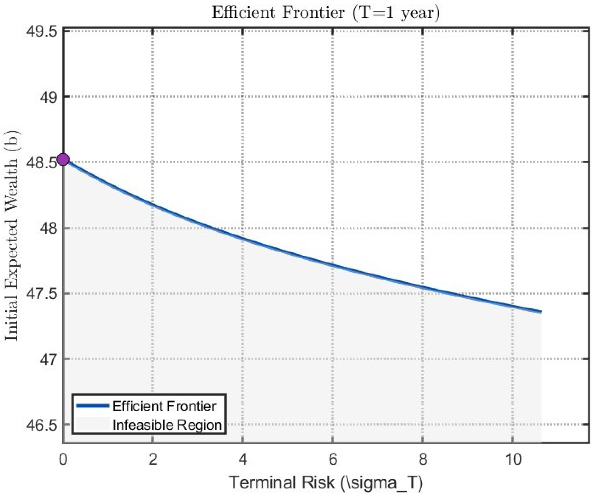
The expected value equality constraint of $E[X_0]=b$ indicates that the expected value of the initial investment portfolio is b. It is an initial reference point set by the investor and is used to measure whether the starting point of the investment portfolio meets the expectations. The variance of the investment portfolio value reflects the extent to which it deviates from the expected path due to factors such as market fluctuations and uncertainties in investment strategies. The larger the variance, the higher the uncertainty of the investment portfolio value is while the greater the investment risk is. Generally, investors hope to minimize this variance under a given expected return level. This leads to solving the following stochastic LQ problem with initial state constraint:

$$\left\{\begin{array}{cccc}\hfill & minVar{X}_T=E{[X_T]}^2-{\left(E[X_T]\right)}^2,\hfill & \hfill & \\ \hfill & subjecttou\in L_{\mathbb{F}}^2(0,T;{\mathbb{R}}^m),\hfill & \\ \hfill & (X_t,u)\mathrm{satisfies}\mathrm{the}\mathrm{CBSLQ}\mathrm{problem}\left(6.1\right)\hfill \end{array}\right.$$

We show in Figure 1 the efficient frontier of the above portfolio management problem for $T=1$ and $\xi =50$. The efficient frontier graph illustrates the trade-off relationship between the initial expected return b and terminal risk (standard deviation), exhibiting a characteristic convex decreasing curve (consistent with high-risk-high-return theory), which validates the core theoretical proposition of the model: precise risk-return management can be achieved through backward stochastic control. The purple point on the graph represents the maximum return point, while the shaded area denotes the infeasible region where no strategy can simultaneously deliver higher returns and lower risk.

Figure 1. Efficient Frontier.

This example visually confirms three key values of the model through the efficient frontier: (1) the initial constraint b enables precise control of the investment starting point; (2) dynamic strategies can generate Pareto-optimal paths; (3) parameters (e.g., the 0.2 adjustment coefficient) possess clear economic significance. In practical applications, this framework provides quantitative tools for structured product design and dynamic pension fund allocation.

7. Conclusions

This paper studies a backward stochastic LQ problem with linear equality constraints on the initial state expectation (CBSLQ). By use of the Lagrange multiplier method and maximum principle, we give an explicit solution to an equivalent unconstrained parameterized BSLQ problem when the cost function is uniformly convex, which is a feedback-optimal control determined by an adjoint SDE, a Riccati-type ODE, a BSDE, and an equality. Under the surjectivity of the linear constraint, we prove the equivalence between the original problem and the dual problem by Lagrange duality theory, thereby obtaining the optimal control for the original CBSLQ. Finally, an illustrative example regarding an investment portfolio is given. This study of the CBSLQ will provide some reference for financial investment or industry control.