Cost Optimization in Sintering Process on the Basis of Bulk Queueing System with Diverse Services Modes and Vacation

Abstract

This research investigated a single bulk server queuing model where service modes and server vacations are dependent on the number of clients. The server operates in three different service modes: single service, fixed batch service, and variable batch service. Modes will be determined by queue length. The service starts only when the minimum number of customers, say ‘a’, has accumulated in the queue. At this point, the server selects one of three service modes. Transitions between duty modes are permitted only at the beginning of a duty period. At the end of the service, the server can go on vacation if the queue length drops below ‘a’. When returning from vacation, if threshold ‘a’ is not reached, the server will remain inactive until it is reached. A special technique called the Supplementary Variables Technique (SVT) was used to determine the probability-generating function when estimating the queue size at a given time. Appropriate numerical examples exemplify the method developed in the paper. An optimal cost analysis was performed to set the threshold values for different server modes with the intention of minimizing the aggregate average cost.

1. Introduction

Several researchers have played a pivotal role in advancing the research on queueing systems involving vacation periods. Notable works feature a single-server queueing system with vacations (see [1,2]), vacation queueing models [3], and a comprehensive survey on single server queues with vacation [4]. In [5], batch queues with extended vacations were analyzed, focusing on the N-policy and multiple vacation scenarios. However, in their model, the server is restricted to serving only one item at a time. In [6], the bulk queueing model with a bulk service rule was introduced. Ref. [7] recently employed the supplementary variable technique to study $M^X/G(a,b)/1$, a model having vacation disruption. Ref. [8] introduced replaceable repair in an M/G/1 new model with threshold and vacation. Ref. [9] provided a review of classical batch arrival and bulk service.

In all the above bulk arrival queueing systems, they considered only one service mode. However, in many practical applications, to reduce congestion, more than one service mode is needed. In such systems, an operator may adjust the server’s service mode depending on the queue length. Ref. [10] explored a method for adapting the service mode in bulk arrival queueing systems according to the current queue length. Their work is based on the Markov decision theorem. This proposed queueing system is unique in that it incorporates three different service modes into a single-server queueing model with vacation periods. Ref. [11] investigated the steady-state conditions and conducted various performance analyses for the M^X/G/1 queueing system, incorporating possible services, postponed repairs, and multiple stages of repair. Ref. [12] employed a supplementary variable technique to study a system represented as $M^X/G(a,b)/1,$ which features multiple vacation periods, closedown times, and optional repairs. Ref. [13] examined a bulk arrival queueing system, focusing on service that depends on batch size and incorporating the concept of a working vacation. In this paper, they also introduced two types of service modes during working vacations.

Ref. [14] examined a non-Markovian bulk service queueing model featuring an unreliable server, N-policy, and Bernoulli-scheduled multiple vacations. Ref. [15] introduced state-dependent breakdowns into a bulk arrival and batch service. By applying the supplementary variable technique, the study derived the probability function for the queue size at any given time, and metrics were calculated and demonstrated through numerical examples. Additionally, a real-time situation in existing healthcare management was also highlighted. Ref. [16] explored phase-dependent breakdowns in a batch service queueing model. Their research introduced two distinct types of breakdowns, each corresponding to one of the two service phases. Ref. [17] introduced a new method for constructing characterization identities for a wide range of absolutely continuous univariate distributions. By extending the explicit formula of the zero-bias distribution within Stein’s method, they obtained clear representations for the distribution function. Instead of concentrating on distributional transformations with particular structures, their focus was on offering formulas that directly capture the distributional properties.

Ref. [18] examined queue-dependent service rates (QDSRs) in the context of a stochastic queueing-inventory system (SQIS). The system includes a single service channel, multiple inventory items, and a finite queue. Customers are served immediately upon arrival if the server is available and adequate inventory is present in the SQIS. Ref. [19] presented a novel closed-form approximation method for analyzing multi-server, single-channel queues with non-Poisson traffic, where inter-arrival and service times follow double-tapering distributions. Ref. [20] explored the analysis of a queueing system with three distinct classes of impatient customers, each defined by its own service time and patience time distributions. They examined the behavior of the system, considering the unique characteristics of these customer classes.

Ref. [21] presented a valuable contribution to the study of queueing systems by extending the M^X/M/C queue to incorporate static and dynamic server groups. The utilization of the difference equations approach and the inclusion of additional features provide a comprehensive framework for analysis. Ref. [22] conducted an in-depth study of the risk-sensitive first passage discounted cost criterion. Their analysis addresses cases involving Borel state and action spaces, accommodating unbounded costs and transition rates. Ref. [23] addressed the issue of limited flow table space in Software-Defined Networking (SDN) switches and its effect on data plane availability. They developed a theoretical model grounded in queueing theory to estimate the state of flow tables in SDN switches, with the goal of offering insights into flow table resource needs and ensuring optimal data plane performance. Ref. [24] explored a dynamic virtual hub location problem within transportation networks. The problem arises when a hub with limited capacity faces, congestion issues, and some or all routes passing through it need to be transferred to a virtual hub to maintain flow connectivity with minimum disruption. The goal was to alleviate congestion at the hubs and ensure a smooth flow of movement throughout the network. The researchers employed the CPLEX optimization software package to solve small sample problems. For large sample sizes, they suggested two metaheuristic algorithms: a genetic algorithm and a competitive algorithm. Ref. [25] investigated a single server queueing model. Within this model, the author introduced a novel approach termed ‘group clearance’, characterized by a general bulk service rule. Notably, this rule allows for an unbounded batch size, enabling the server to process tasks in exceptionally large groups.

Ref. [26] tackled peak-hour congestion in urban rail stations by introducing a simulation-based optimization method for managing passenger flow. Their approach leverages queueing networks and surrogate models to optimize flow control strategies to enhance station throughput, reduce congestion, and improve passenger experience. A two-stage process combines multi-agent simulation, a Kriging model, and particle swarm optimization to manage ingress flow, tested on Zhongguancun Station in Beijing. Results show the method reduces wait times, conserves resources, and supports a sustainable transit system. Ref. [27] addressed challenges in bus charging stations (CSs) caused by increased demand from private vehicles, such as high electricity costs and long wait times. A dual-layer optimization model, leveraging the Golden Sine Algorithm, was used to balance construction and user costs. By integrating energy storage scheduling with an M/M/c queue model, the study sought to reduce grid load and minimize wait times. Results show a 6% reduction in electricity costs and a drop in average waiting time to 2.1 min, offering a promising solution for a more efficient and sustainable bus CS operation. Ref. [28] addresses the challenge of dynamic real-time task offloading in a multi-user Mobile Edge Computing (MEC) network, aiming to optimize energy consumption while ensuring long-term system stability. By applying Lyapunov theory to decouple the problem and framing it as a Markov decision process, the study introduced a deep reinforcement learning (DRL)-based LMADDPG algorithm to enhance task-offloading decisions. The simulation results show that this approach improves performance over baseline algorithms in managing offloading tasks under energy constraints, ensuring better user experience and system efficiency. Ref. [29] presents a multi-period queuing location-allocation model. This model optimizes facility locations and transportation using M/M/C/K queuing systems to improve profitability, decrease driver wait times, and minimize environmental impact. A mixed-integer nonlinear programming (MINLP) approach was utilized, with the grasshopper optimization algorithm (GOA) offering a more efficient solution to large-scale problems compared with traditional methods like GAMS. The findings indicate that GOA performs similarly to GAMS while significantly reducing processing times and effectively balancing costs, environmental impact, and wait times. Ref. [30] presented a queueing system where customers arrive in bulk according to a Poisson process, and the service was divided into two phases: First Essential Service and Second Essential Service, with varying server capacities. Feedback after the Second Essential Service, server vacations, and system renewals was modeled with respective probabilities. The supplementary variable technique was used to derive the probability-generating function of the queue size at arbitrary times, and numerical examples were provided to illustrate the analytical results. This model addresses server utilization and dynamic queue management under various conditions.

Modeling and analysis of queueing systems with vacation play an important role in dealing with real-life congestion problems. The utilization of idle time in the bulk arrival queueing model makes systems much more realistic and flexible. These types of queueing models have practical applications in various fields, including manufacturing industries, production line systems, and communication networks. The inspiration for this particular model stems from a real-life scenario in pharmaceutical science, specifically related to the sintering process used in tablet production. Sintering is a technique that involves heating powdered material in a furnace below its melting point until the particles bond together. In this process, the components of the tablets are the customers arriving for the sintering process. The sintering furnace is the server where the components are compressed and manufactured tablets. The service mode of the server can be changed by the operator based on queue length.

In this model, the input to the sintering process arrives in batches, which are then collectively subjected to the sintering furnace for bulk treatment. The activation of the furnace hinges on the availability of a sufficient batch size, as it is optimized for larger loads. Once initiated, the furnace operation needs to be maintained consistently over multiple successive batches to avoid an escalation in operational expenses. Upon the completion of the sintering process, if the remaining components fall short of a predefined batch size ‘a’, the operator halts the sintering process and undertakes a secondary task. This secondary task could encompass activities like blending powders for subsequent procedures, cleaning external surfaces, and verifying component dimensions. Subsequent to the secondary task, the operator remains within the system, awaiting the arrival of the necessary components. This intricate sintering process can be effectively represented as a bulk queueing system characterized by a range of service modes and instances of operational downtime.

In this model, service is provided in three modes: single service, fixed batch service, and variable batch service. Even a single service will only begin when the queue length reaches ‘1000 grams’ (customers). A queue size-dependent service approach is necessary to minimize the costs. Changes in the service mode can only occur at the start of a service period. Variable batch service is available only when the queue length reaches ‘2000 grams’(customers) (2000 > 1000) and is provided based on the general bulk service rule, with batch sizes ranging from a minimum of ‘2000 grams’(customers) to a maximum of ‘4000 grams’(customers). Similarly, the server offers fixed batch service when the queue length is at least ‘10,000 grams’ (customers) (10,000 > 4000), where ‘4000 grams’ (customers) is the upper limit for varying batch service. In fixed batch service, a predetermined batch size of ‘5000 grams’ (customers) is used. After each service completion, the service mode may either change or remain the same. If the queue length is less than ‘1000 grams’ (customers), the server goes on vacation. Upon returning from vacation, the service process is reinitiated. If the queue length is still below ‘1000 grams’ (customers), the server stays idle (dormant period) until the queue length reaches the threshold required to start the service.

The main contributions of this study include the following:

• We introduce three service modes for a bulk queueing system based on queue length with the intention of reducing the waiting time of customers in the queue.
• Single service, fixed batch service, and variable batch service are incorporated into the same server to minimize the total average cost of the system.
• Modeling a bulk queueing system with fixed batch service as one of the service modes plays a vital role in reducing the operating cost of the system.
• An application for the proposed model is explained in detail based on powder metallurgy (sintering process).

The paper is structured as follows: Section 1 presents the introduction and literature review. In Section 2, the model description and methodology for the proposed queuing model are detailed. Section 3 provides the stochastic model, governing equations, queue size distribution, performance measures, and special cases. Section 4 focuses on the cost model for the system and includes numerical illustrations. Finally, Section 5 offers the conclusion and suggestions for future work.

2. Model and Methods

2.1. Arrival Process

The arrival process describes how entities enter the system. In our work, customers arrive in batches according to a Poisson process with an arrival rate $\tau$. The time between arrivals follows a specific pattern: group sizes are distributed according to a geometric distribution, while inter-arrival times follow an exponential distribution.

2.2. Service Process

The service process outlines how the server attends to customers. In this model, the server operates in three distinct modes: single service and batch service, with either a fixed or variable batch size, following the general bulk service rule. The service time is governed by a general distribution.

2.3. Single Service

At a given time instant, if the server is able to serve only one customer at a time, then such type of service is called a single service.

2.4. Fixed Batch Service

When the server provides service in batches with fixed batch size ‘K’, then the service process is said to be a fixed batch service.

2.5. Variable Batch Service

In variable batch service, customers are served in batches with different batch sizes according to the general bulk service rule [6].

2.6. Vacation

After completing the service, if the queue length drops below the threshold ‘a’, then the server goes on vacation (secondary job). To make use of this idle time, the server is assigned a secondary task (vacation), which may improve the quality of future service.

2.7. Dormant Period

After the vacation completion, if the queue length is still below this threshold, the server remains idle (dormant) until it reaches ‘a’.

2.8. Description of the Model

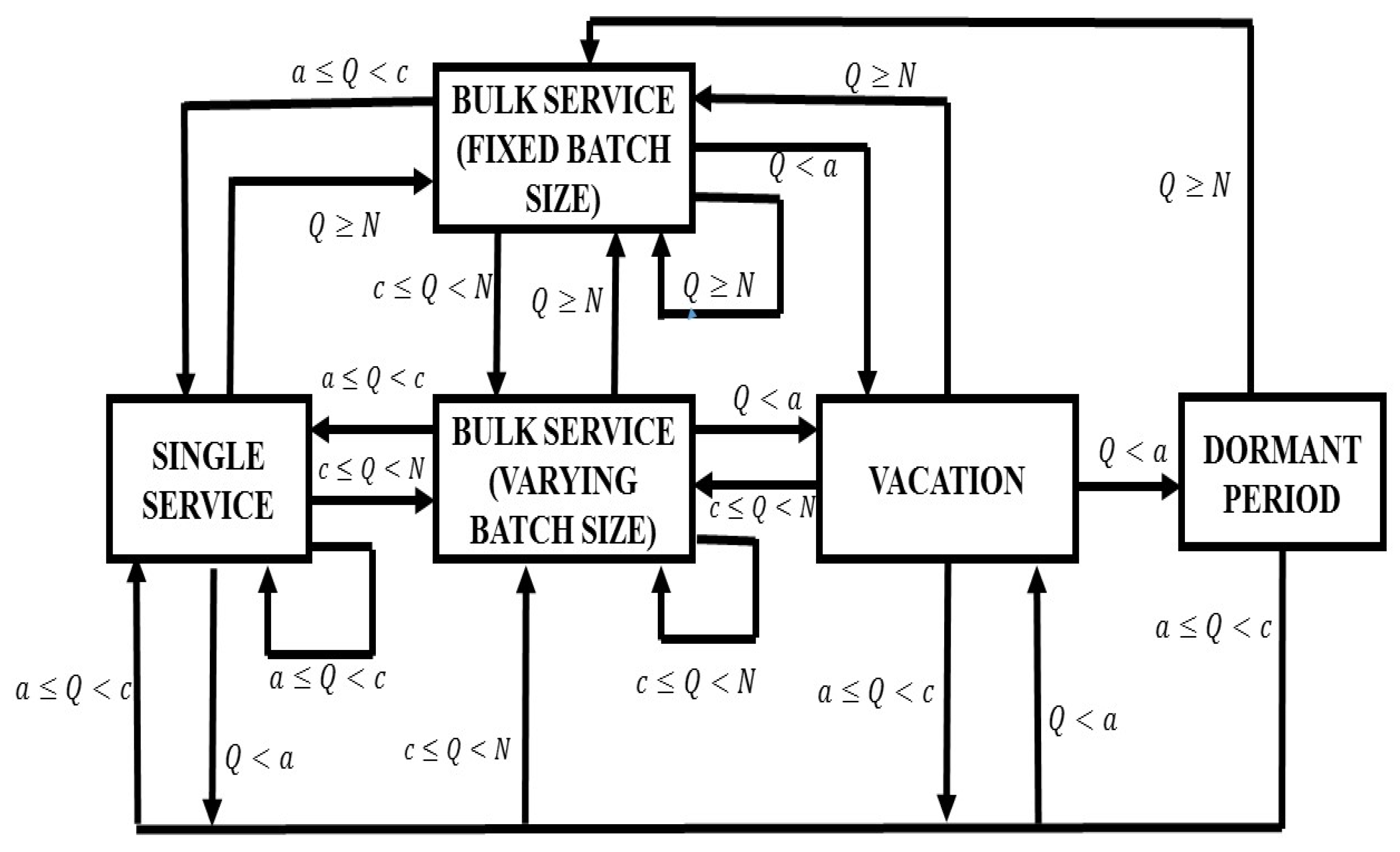
This paper examines a bulk arrival queueing model with different service modes and server vacations. The system offers three service modes: single service, fixed batch service, and variable batch service, depending on the queue length. Even a single service will commence only when the queue length reaches a specific value, ‘a’. To minimize the system’s aggregate mean cost, queue size dependent service is implemented. The service mode can only be changed at the initiation of a service period. Variable batch service is available only when the queue length reaches ‘c’ (where c > a) and is provided based on the general bulk service rule introduced by [6], with batch sizes ranging from a minimum of ‘c’ to a maximum of ‘b’ items. Similarly, if the queue length is at least ‘N’ (N > b), where ‘b’ is the maximum batch size for variable batch service, the server offers constant batch service. Services will be rendered in accordance with a predetermined batch size ‘k’ in fixed batch services. After each service completion, the service mode may change or remain unchanged based on the current queue length. Because the switching over time in this system is so small, it is not considered. If the queue length is smaller than ‘a’ at the time the service is completed, the server goes on vacation. Depending on how long the queue is, the service process will begin after a vacation. If the queue length is still less than ‘a’ even after the vacation is over, the server stays dormant time until the queue length crosses the threshold value needed to initiate service. Figure 1 shows a schematic representation of this suggested system.

2.9. Methodology

The proposed queueing model is non-Markovian in nature. Therefore, we used the supplementary variable technique (SVT) and remaining service time as a supplementary variable to derive the PGF of queue size at an arbitrary time.

2.10. Notations

Let W denote the random variable representing the group size of arrivals. Let P(Z) be the probability-generating function (PGF) of Z, $g_k$ the probability that a batch arrives ‘k’ customers, and $\tau$ the Poisson arrival rate. Other notations are presented in

Table 1. Notation used in the paper.

S = Service	Cumulative Distribution Function	Probability Density Function	Laplace-Stieltjes Transform (LST)	Remaining Service Time
Variable batch S	$B_1(w)$	$b_1(w)$	${\tilde{B}}_1(\mathsf{\delta })$	${B_1}^0$(w)
Fixed batch S	$B_2(w)$	$b_2(w)$	${\tilde{B}}_2(\mathsf{\delta })$	${B_2}^0$(w)
Single S	A(w)	a(w)	$\tilde{\mathrm{A}}(\mathsf{\delta }$)	${\mathrm{A}}^0$(w)
Vacation	Q(w)	q(w)	$\tilde{\mathrm{Q}}(\mathsf{\delta }$)	${\mathrm{Q}}^0$(w)

.

With $C_q\left(t\right)$, the count of customers awaiting service is noted, and with $C_s\left(t\right)$, the number of customers currently being served at time t is noted.

$$\psi —\left(t\right)=\left\{\begin{array}{c}0, when the server is busy with varying batch service\\ 1, when the server is busy with fixed batch service \\ 2, when the server is busy with single service \\ 3, when the server is on vacation\\ 4, when the server is on dormant period \end{array}\right.$$

The State Probabilities are defined as follows:

$$V_{ij}(w,t)\mathit{dt}=P_r\left\{\begin{array}{c}{C}_s\left(t\right)=i, C_q\left(t\right)=j, \\ w\le {B_1}^0\left(t\right)\le w+dt,\psi \left(t\right)=0\end{array}\right\}, a\le i\le b; j \ge 1$$

$$F_{kj}(w,t)\mathit{dt}=P_r\left\{\begin{array}{c}{C}_s\left(t\right)=k, C_q\left(t\right)=j,\\ w\le {B_2}^0\left(t\right)\le w+dt,\psi \left(t\right)=1\end{array}\right\}, j\ge 1, k\le N(fixed batch size);$$

$${ S}_{1n}(w, t)\mathit{dt}=P_r\left\{\begin{array}{c}{C_s\left(t\right)=1,C}_q\left(t\right)=n, \\ y\le A^0\left(t\right)\le y+dt,\psi \left(t\right)=2\\ \end{array}\right\}, n\ge 1;$$

$$Q_n(w,t)\mathit{dt}=P_r\left\{\begin{array}{c}{C}_q\left(t\right)=n, \\ w\le Q^0\left(t\right)\le w+dt\\ \end{array}, \psi \left(t\right)=3\right\}, 0\le n\le a-1;$$

$$T_n\left(t\right)=P_r\left\{N_q\left(t\right)=n,\right.\left.\psi \left(t\right)=4\right\}, 0\le n\le a-1.$$

3. Results

3.1. System Analysis

The governing equations of the model are obtained using the method of SVT.

$$\begin{gathered} -{\displaystyle \frac{d}{dx}} S_{1a-1}(w)=-\tau S_{1a-1}\left(w\right)+{\sum }_{m=c}^b{V}_{ma}\left(0\right)a(w) \\ +S_{1a}(0)a(w)+{\sum }_{k=1}^{a-1}{T}_k\tau g_{a+1-k} a\left(w\right)+Q_a\left(0\right)a\left(w\right)+F_{ka}\left(0\right)a\left(w\right); \end{gathered}$$

(1)

Equation (1) denotes the different probabilities for the server in a single service with ‘1’ customers in service and ‘a − 1’ customers in the queue in the remaining service time w − ∆t at time t + ∆t. In RHS, the first term indicates that there is no arrival at that time, and the second term indicates that when variable batch service is completed, if ‘a’ customers are in the queue, then ‘m’ customers go for variable batch service and ‘a − 1’ customers are waiting in the queue. The next term indicates that when single service is completed, if ‘a’ customers are in the queue, then ‘1’ customers go for a single service, and ‘a − 1’ customers will be waiting in the queue. The fourth term indicates that during the dormant period, if k customers are in the queue, then a + 1 − k customers may enter the queue. After vacation completion, if ‘a’ customers are in the queue, then ‘1’ customers go for a single service, and ‘a − 1’ customers will be waiting in the queue, and the last term indicates that when fixed batch service is completed, if ‘a’ customers are in the queue, then ‘k’ customers go for fixed batch service, and ‘a − 1’ customers will be waiting in the queue. Similarly, Equations (2)–(14) can be expressed with the help of a schematic representation of the queueing model (Figure 1).

$$\begin{gathered} -{\displaystyle \frac{d}{dx}}{S}_{1n}\left(w\right)=-\tau S_{1n}\left(w\right)+S_{1n+1}\left(0\right)a\left(w\right)+\sum _{m=c}^b{V}_{m,n+1}\left(0\right)a\left(w\right)+F_{k,n+1}\left(0\right)a\left(w\right) \\ +{\sum }_{k=0}^{a-1}{T}_k \tau { g}_{n+1-k}a(w)+{\sum }_{k=1}^{n-a}{S}_{1 n-k}\left(w\right) \tau g_k{+Q}_{n+1}\left(0\right)a\left(w\right), a\le n \le c-2; \end{gathered}$$

(2)

$$\begin{gathered} -{\displaystyle \frac{d}{dx}}{S}_{1n}\left(w\right)=-\tau S_{1n}\left(w\right)+\sum _{k=1}^{n-a}{S}_{1 n-k}\left(w\right) \tau g_k \\ + {\sum }_{k=0}^{a-1}{T}_k\tau g_{n+1-k }a\left(w\right)+Q_{n+1}\left(0\right)a\left(w\right), n=c-1; \end{gathered}$$

(3)

$$-{\displaystyle \frac{d}{dx}}{S}_{1n}\left(w\right)=-\tau H_{1n}\left(w\right)+\sum _{k=1}^{n-a}{S}_{1 n-k}\left(w\right) \tau g_{k }, n \ge c;$$

(4)

$$\begin{gathered} -{\displaystyle \frac{d}{dx}}{V}_{i0}\left(w\right)=-\tau V_{i0} \left(w\right)+{\sum }_{m=0}^{a-1}{T}_m\tau g_{i-m}{b}_1\left(w\right) \\ +\sum _{m=c}^b{V}_{mi}\left(0\right)b_1\left(w\right)+S_{1i}\left(0\right)b_1\left(w\right)+F_{ki}\left(0\right)b_1\left(w\right)+Q_i\left(0\right)b_1\left(w\right), c \le i \le b; \end{gathered}$$

(5)

$$-{\displaystyle \frac{d}{dx}}{V}_{ij}\left(w\right)=-\tau V_{ij}\left(w\right)+\sum _{k=1}^j{V}_{i j-k}\left(w\right) \tau g_k, c \le i \le b-1 , j \ge 1;$$

(6)

$$-{\displaystyle \frac{d}{dx}}{V}_{bj}\left(w\right)=-\tau V_{bj}\left(w\right)+\sum _{k=1}^j{V}_{b j-k}\left(w\right) \tau g_k+\sum _{m=c}^b{V}_{mb+j}\left(0\right)b_1\left(w\right),$$

(7)

$$+S_{1b+j}(0) b_1(w{\sum }_{m=0}^{a-1}{T}_m{g}_{b+j-m}{b}_1\left(w\right)+Q_{b+j}\left(0\right)b_1\left(w\right)+F_{kb+j}\left(0\right)b_1\left(w\right), j \ge 1;$$

$$\begin{gathered} -{\displaystyle \frac{d}{dx}}{F}_{k0}\left(w\right)=-\tau F_{k0}\left(w\right)+S_{1j}\left(0\right)b_2\left(w\right)+Q_j\left(0\right)b_2\left(w\right) \\ +{\sum }_{m=c}^b{V}_{mj}\left(0\right)b_2\left(w\right)+{\sum }_{j=k}^N{F}_{kj}\left(0\right)b_2\left(w\right)+{\sum }_{m=0}^{a-1}{T}_m\tau g_{j-m}{b}_2\left(w\right), j\ge N; \end{gathered}$$

(8)

$$\begin{gathered} -{\displaystyle \frac{d}{dx}}{F}_{kj}\left(w\right)=-\tau F_{kj}\left(w\right)+S_{1K+j}\left(0\right)b_2\left(w\right)+{\sum }_{m=1}^j{F}_{k j-m}\left(w\right)\tau g_m{+Q}_{k+j}\left(0\right)b_2\left(w\right) \\ +{\sum }_{m=c}^b{V}_{m k+j}\left(0\right)b_2\left(w\right)+{\sum }_{j=k}^N{F}_{k k+j}\left(0\right)b_2\left(w\right)+{\sum }_{m=0}^{a-1}{T}_m\tau g_{k+j-m}{b}_2\left(w\right), j \ge N, \end{gathered}$$

(9)

$$-{\displaystyle \frac{d}{dx}}{Q}_0\left(w\right)=-\tau Q_0\left(w\right)+{\sum }_{m=c}^b{V}_{m0}\left(\right)qw+F_{k0}\left(0\right)q\left(w\right)+S_{10}\left(0\right)q\left(w\right);$$

(10)

$$\begin{gathered} -{\displaystyle \frac{d}{dx}}{Q}_n\left(w\right)=-\tau Q_n\left(w\right)+ {\sum }_{m=c}^b{V}_{mn}(0)q(w)+F_{kn}\left(0\right)q()+{\sum }_{k=1}^n{Q}_{n-k}\left(w\right)\tau g_k, \\ 1\le n\le a-1 \end{gathered}$$

(11)

$$\begin{array}{c}\hfill -{\displaystyle \frac{d}{dx}}{Q}_n\left(w\right) =-\tau Q_n\left(w\right)+{\sum }_{m=c}^b{V}_{mn}(0)q(w)+F_{kn}\left(0\right)q\left(w\right)+S_{1n}\left(0\right)q\left(w\right)\\ \hfill +{\sum }_{k=1}^n{Q}_{n-k}\left(w\right)\tau g_k, n=a-1;\end{array}$$

(12)

$$0=-\tau T_0 + Q_0\left(0\right),$$

(13)

$$0=-\tau T_n+Q_n\left(0\right)+{\sum }_{k=1}^n{T}_{n-k}\tau g_k , 1 \le n \le a-1;$$

(14)

LST of ${\tilde{S}}_{1n}(\delta )$, ${\tilde{V}}_{in}(\delta )$, ${\tilde{F}}_k(\delta )$ and ${\tilde{Q}}_n(\delta )$ are defined as:

$$\begin{gathered} {\tilde{S}}_{1n}\left(\delta \right)={\int }_0^{\infty }{e}^{-\delta x}{S}_{1n}(w)dw; {\tilde{V}}_{in}(\delta ) {\int }_0^{\infty }{e}^{-\delta x}{V}_{in}\left(w\right)dw; \\ {\tilde{Q}}_n\left(\delta \right)={\int }_0^{\infty }{e}^{-\delta x}{Q}_n\left(w\right)dw; {\tilde{F}}_k(\delta )={\int }_0^{\infty }{e}^{-\delta x}{F}_k(w)dw. \end{gathered}$$

Taking LST on both sides from Equations (1)–(14), it obtains the following:

$$\delta {\tilde{S}}_{ia-1}\left(\delta \right)-S_{1a-1}\left(0\right)=\tau {\tilde{S}}_{1a-1}\left(\delta \right)-\tilde{A}\left(\delta \right)[{\sum }_{k=1}^{a-1}{T}_k\tau g_{a+1-k}+Q_a\left(0\right)+F_{ka}\left(0\right)+\sum _{m=c}^b{V}_{ma}\left(0\right)+S_{1a}\left(0\right),$$

(15)

$$\begin{gathered} \delta {\tilde{S}}_{in}\left(\delta \right)-S_{1n}\left(0\right)=\tau {\tilde{S}}_{1n}\left(\delta \right)-{\sum }_{k=1}^{n-a}{\tilde{S}}_{1 n-k}\left(\delta \right) \tau g_k-A\left(\delta \right)\left[{\sum }_{k=0}^{a-1}{T}_k\tau g_{n+1-k}+Q_{n+1}\left(0\right)\right], \\ a\le n \le c-2; \end{gathered}$$

(16)

$$\delta {\tilde{\mathrm{S}}}_{\mathrm{i}\mathrm{n}}\left(\delta \right)-S_{1n}\left(0\right)=\tau {\tilde{S}}_{1n}\left(\delta \right)-{\sum }_{k=1}^{n-a}{\tilde{S}}_{1 n-k}\left(\delta \right) \tau g_k-A\left(\delta \right)\left[{\sum }_{k=0}^{a-1}{T}_k\tau g_{n+1-k}+Q_{n+1}(0)\right], n=c-1;$$

(17)

$$\delta {\tilde{S}}_{in}\left(\delta \right)-S_{1n}\left(0\right)=\tau {\tilde{S}}_{1n}\left(\delta \right)-{\sum }_{k=1}^{n-a}{\tilde{S}}_{1 n-k}\left(\delta \right)\tau g_k, n\ge c;$$

(18)

$$\begin{gathered} \delta {\tilde{V}}_{i0}\left(\delta \right)-V_{i0}\left(0\right)=\tau {\tilde{V}}_{io}\left(\delta \right)-Q_i\left(0\right){\tilde{B}}_1\left(\delta \right)-{\tilde{B}}_1\left(\delta \right)\left[{\sum }_{m=0}^{a-1}{T}_m\tau g_{i-m}+S_{1i}\left(0\right)+{\sum }_{m=c}^b{V}_{mi}\left(0\right)+F_{k,i}\left(0\right)\right], \\ c\le i\le b; \end{gathered}$$

(19)

$$\delta {\tilde{\mathrm{V}}}_{\mathrm{i}\mathrm{j}}\left(\delta \right)-V_{ij}\left(0\right)=\tau {\tilde{V}}_{ij}\left(\delta \right)-{\sum }_{k=1}^j{\tilde{V}}_{i j-k}\left(\delta \right) \tau g_k, c\le i\le b-1$$

(20)

$$\begin{gathered} \delta {\tilde{V}}_{bj}\left(\delta \right)-V_{bj}\left(0\right)=\tau {\tilde{V}}_{bj}\left(\delta \right)-\sum _{k=1}^j{\tilde{V}}_{b j-k}\left(\delta \right) \tau g_k \\ -{\tilde{B}}_1(\delta )[{\sum }_{m=c}^b{V}_{mb+j}\left(0\right)+S_{1b+j}\left(0\right)+{\sum }_{m=0}^{a-1}{T}_m\tau g_{b+j-m}+Q_{b+j}\left(0\right)+F_{k,b+j}\left(0\right)], \end{gathered}$$

(21)

$$\delta {\tilde{F}}_{k0}\left(\delta \right)-F_{k0}\left(0\right)=\tau {\tilde{F}}_{k0}\left(\delta \right)-{\tilde{B}}_2\left(\delta \right)\left[Q_j\left(0\right)+{\sum }_{m=0}^{a-1}{T}_m\tau g_{j-m}+{\sum }_{m=c}^b{V}_{mj}\left(0\right)+{\sum }_{j=k}^N{F}_{kj}\left(0\right)\right], j \ge 1;$$

(22)

$$\begin{gathered} \delta {\tilde{F}}_{kj}\left(\delta \right)-F_{kj}\left(0\right)=\tau {\tilde{F}}_{kj}\left(\delta \right)-{\sum }_{m=1}^j{\tilde{F}}_{k j-m}\left(\delta \right)\tau g_m- \\ {\tilde{B}}_2\left(\delta \right)\left[S_{1 K+j}\left(0\right){+Q}_{k+j}\left(0\right)+{\sum }_{m=c}^b{V}_{m k+j}\left(0\right)+{\sum }_{j=k}^N{F}_{k k+j}\left(0\right)+{\sum }_{m=0}^{a-1}{T}_m\tau g_{k+j-m}\right], j\ge N; \end{gathered}$$

(23)

$${\tilde{\mathrm{Q}}}_0\left(\delta \right)-Q_o\left(0\right)=\tau {\tilde{Q}}_0\left(\delta \right)-\tilde{Q}\left(\delta \right)\left[{\sum }_{m=c}^b{V}_{m0}\left(0\right)+F_{k0}\left(0\right)+S_{10}\left(0\right)\right] ;$$

(24)

$$\begin{gathered} \delta {\tilde{Q}}_n\left(\delta \right)-Q_n\left(0\right)=\tau {\tilde{Q}}_n\left(\delta \right)-{\sum }_{k=1}^n{\tilde{Q}}_{n-k}(\delta ) \tau g_k-\tilde{Q}(\delta )\left[ {\sum }_{m=c}^b{V}_{mn}\left(0\right)+F_{kn}\left(0\right)\right], \\ 1\le n\le a-1; \end{gathered}$$

(25)

$$\begin{gathered} \delta {\tilde{Q}}_n\left(\delta \right)-Q_n\left(0\right)=\tau {\tilde{Q}}_n\left(\delta \right)-{\sum }_{k=1}^n{\tilde{Q}}_{n-k}(\delta ) \tau g_k-\tilde{Q}(\delta )[ {\sum }_{m=c}^b{V}_{mn}\left(0\right)+F_{kn}\left(0\right)+S_{1n}\left(0\right)], \\ n=a-1. \end{gathered}$$

(26)

3.2. Probability-Generating Function (PGF)

The functions that generate the probability of various states are defined below:

$$\tilde{S}(z, \delta )={\sum }_{n=a-1}^{\infty }{\tilde{S}}_{in}(\delta )z^n ; S(z, 0)={\sum }_{n=a-1}^{\infty }{S}_{in}(0)z^n;$$

$${\tilde{V}}_i\left(z, \delta \right)=\sum _{j=0}^{\infty }{\tilde{V}}_{i,j}\left(\delta \right)z^j; V_i\left(z, 0\right)=\sum _{j=0}^{\infty } V_{ij} \left(0\right)z^j;$$

$$\tilde{Q}\left(z, \delta \right)=\sum _{n=0}^{a-1} {\tilde{Q}}_n\left(\delta \right)z^n; Q \left(z, 0\right)=\sum _{n=0}^{a-1}{Q}_n \left(0\right)z^n;$$

$${\tilde{F}}_k\left(z, \delta \right)=\sum _{j=N}^{\infty }{\tilde{F}}_{k,j}\left(\delta \right)z^j; F_k\left(z, 0\right)=\sum _{j=N}^{\infty } F_{kj} \left(0\right)z^j$$

$$k\le N, fixed batch size.$$

$$\mathrm{T}\left(\mathrm{z}\right)\sum _{n=0}^{a-1}{T}_n{z}^n, c \le i \le b.$$

(27)

By taking Z—transforms of the above Equations (15)–(26) and then using (27), we obtain the following:

$$\begin{gathered} \left(\delta -\tau +\tau W\left(z\right)\right)\tilde{S}\left(\mathrm{z},\delta \right)=\mathrm{S}\left(\mathrm{z},0\right)-{\tilde{A}\left(\delta \right)[Q}_n\left(0\right)+S_{1n}\left(0\right)+F_{kn}\left(0\right){\sum }_{m=0}^{a-1}{T}_m\tau g_{n-m}]z^{n-1} \\ -\tilde{A}\left(\delta \right)[\left({\sum }_{m=c}^b{V}_{mn}\left(0\right)\right)z^{n-1}] a \le n \le c-1 \end{gathered}$$

(28)

$$\begin{gathered} \left(\delta -\tau +\tau W\left(z\right)\right){\tilde{V}}_i\left(\mathrm{z},\delta \right)={\mathrm{V}}_{\mathrm{i}}\left(\mathrm{z},0\right)-{\tilde{B}}_1\left(\delta \right)\left[{\sum }_{m=0}^{a-1}{T}_m\tau g_{i-m}+S_{1i}\left(0\right)+Q_i\left(0\right)\right] \\ -{\tilde{B}}_1(\delta )[ {\sum }_{m=c}^b{V}_{mi}\left(0\right)+F_{k,i}(0)], c \le i \le b-1 \end{gathered}$$

(29)

$$\begin{gathered} z^b\left(\delta -\tau +\tau W \left(z\right)\right){\tilde{V}}_b\left(z, \delta \right)=z^b{V}_b(z, 0)-{\tilde{B}}_1(\delta )[\left({\sum }_{m=c}^b{V}_m\left(z,0\right)-{\sum }_{j=0}^{b-1}{V}_{mj }\left(0\right)z^j\right)]-{\tilde{B}}_1(\delta )[ S\left(z,0\right)-{\sum }_{n=a-1}^{b-1}{S}_{1n}\left(0\right)z^n+Q\left(z,0\right)-{\sum }_{n=0}^{b-1}{Q}_n\left(0\right)z^n+F_k\left(z,0\right)-{\sum }_{n=0}^{b-1}{F}_n\left(0\right)z^n] \\ -{\tilde{B}}_1(\delta )[\lambda \left(T\left(z\right)W\left(z\right)-{\sum }_{m=0}^{c-1}\left(T_m{z}^m{\sum }_{j=1}^{b-m-1}{g}_j{z}^j\right)\right)]; \end{gathered}$$

(30)

$$\begin{gathered} \left(\delta -\tau +\tau W\left(z\right)\right)\tilde{Q}\left(\mathrm{z},\delta \right)=Q\left(z,0\right)-\tilde{Q}(\delta )[{\sum }_{m=c}^b{V}_{mn}\left(0\right)+F_{kn}\left(0\right)+S_{1n}\left(0\right)]z^n \\ 1\le n\le a-1, \end{gathered}$$

(31)

Let $s_n={\sum }_{n=a-1}^{b-1}{S}_{1n}\left(0\right)$; $q_n={\sum }_{n=0}^{b-1}{Q}_n\left(0\right)$; $v_j={\sum }_{j=0}^{b-1}{V}_{mj}\left(0\right); f_n={\sum }_{n=0}^{b-1}{F}_n\left(0\right)$

$$\begin{gathered} {\mathrm{z}}^{\mathrm{k}}\left(\mathsf{\delta }-\mathsf{\tau }+\mathsf{\tau }\mathrm{W}\left(\mathrm{z}\right)\right){\tilde{\mathrm{F}}}_{\mathrm{k}}\left(\mathrm{z},\mathsf{\delta }\right)={(\mathrm{z}}^{\mathrm{k}}-{\tilde{\mathrm{B}}}_2(\mathsf{\delta })){\mathrm{F}}_{\mathrm{k}}(\mathrm{z},0) \\ {-\tilde{B}}_2\left(\delta \right)[S\left(z,0\right)+{\sum }_{m=c}^{b-1}{V}_m\left(z, 0\right)+Q\left(z,0\right)-{\sum }_{j=0}^{N-1}{(s}_n+q_n+f_n+v_n)z^j+\tau \left(T\left(z\right)W\left(z\right)-{\sum }_{m=0}^{k-1}\left(T_m{z}^m{\sum }_{j=1}^{N-m-1}{g}_j{z}^j\right)\right). \end{gathered}$$

(32)

It is assumed that P(z) is the function that generates the probability of the queue size at any time. Then, the following is true:

$$P (z)={\sum }_{m=c}^{b-1}{\tilde{V}}_m(z,0)+{\tilde{V}}_b(z, 0)+\tilde{Q} (z, 0)+{\tilde{F}}_k(z,0)+T (z)+\tilde{S} (z, 0)$$

(33)

By substituting $\mathsf{\delta }=\tau -\tau \mathrm{W}(\mathrm{z})$ in Equations (28)–(32), without loss of generality and proper manipulation of generating function for different states, Equation (33) is simplified. We denote the following:

$$\begin{gathered} A=\left({\sum }_{i=c}^{b-1}{c}_i+q_i+M_2\right)\Psi \left({\tilde{B}}_1,{\tilde{B}}_2\right)+\left({\sum }_{i=a}^{c-1}{(c}_i+q_i+M_2)z^{i-1}\right)\Phi \left({\tilde{B}}_1,{\tilde{B}}_2,\tilde{A}\right)+ \\ \left(\gamma \left({\tilde{B}}_1,{\tilde{B}}_2,\tilde{Q}\right)\right){\sum }_{i=0}^{a-1}{c}_i{z}^i+F\left(z\right)+M_4; {B=M}_3\left(-\tau +\tau W\left(z\right)\right); \end{gathered}$$

It results as follows:

$$P\left(z\right)={\displaystyle \frac{A}{B}},$$

(34)

where:

$$\begin{gathered} \Psi \left({\tilde{B}}_1,{\tilde{B}}_2\right)=z^k\left({\tilde{B}}_1\left(\tau -\tau W\left(z\right)\right)-1\right)+({\tilde{B}}_2\left(\tau -\tau W\left(z\right)\right)-{\tilde{B}}_1\left(\tau -\tau W\left(z\right)\right)) \\ +M_1{z}^{-b}\left(z^k\left({\tilde{B}}_1\left(\tau -\tau W\left(z\right)\right)-1\right){-M}_1+{\tilde{B}}_2\left(\tau -\tau W\left(z\right)\right)\right)\Phi \left({\tilde{B}}_1,{\tilde{B}}_2,\tilde{A}\right) \\ =M_1{z}^{-b}\tilde{A}(\tau -\tau W\left(z\right))\left(z^k-{\tilde{B}}_2\left(\tau -\tau W\left(z\right)\right)-1\right)-z^{-b}{\tilde{B}}_2\left(\tau -\tau W\left(z\right)\right)\tilde{A}(\tau -\tau W\left(z\right))\left(z^k-1\right) \\ +z^{k-b}\left({\tilde{B}}_1\left(\tau -\tau W\left(z\right)\right)-\tilde{A}\left(\tau -\tau W\left(z\right)\right)\right)+z^{-b}\tilde{A}\left(\tau -\tau W\left(z\right)\right)\left({\tilde{B}}_1\left(\tau -\tau W\left(z\right)\right)-z^b\right)-z^{-b}{M}_1 \\ +z^{-b}{\tilde{B}}_2\left(\tau -\tau W\left(z\right)\right)\left({\tilde{B}}_2\left(\tau -\tau W\left(z\right)\right)\tilde{A}\left(\tau -\tau W\left(z\right)\right)\right)-z^{-b}\left(\tilde{A}\left(\tau -\tau W\left(z\right)\right)-1\right)\left({z^b\tilde{B}}_2\left(\tau -\tau W\left(z\right)\right)+z^{b+k}\right); \end{gathered}$$

$$\begin{gathered} \gamma \left({\tilde{B}}_1,{\tilde{B}}_2,\tilde{Q}\right)=z^{-b}{M}_1\tilde{A}(\tau -\tau W\left(z\right))\left(z^k-{\tilde{B}}_2\left(\tau -\tau W\left(z\right)\right)-1\right) \\ -z^{-b}{\tilde{B}}_2\left(\tau -\tau W\left(z\right)\right)\tilde{A}(\tau -\tau W\left(z\right))\left(z^k-1\right)+z^{k-b}\left({\tilde{B}}_1\left(\tau -\tau W\left(z\right)\right)-\tilde{A}\left(\tau -\tau W\left(z\right)\right)\right) \\ +z^{-b}\tilde{A}\left(\tau -\tau W\left(z\right)\right)\left({\tilde{B}}_1\left(\tau -\tau W\left(z\right)\right)-z^b\right)-{z^{-b}M}_1+z^{-b}{\tilde{B}}_2\left(\tau -\tau W\left(z\right)\right)\left({\tilde{B}}_2\left(\tau -\tau W\left(z\right)\right)\tilde{A}\left(\tau -\tau W\left(z\right)\right)\right) \\ -z^{-b}\left(\tilde{A}\left(\tau -\tau W\left(z\right)\right)-1\right)\left({z^b\tilde{B}}_2\left(\tau -\tau W\left(z\right)\right)+z^{b+k}\right)+\left(\tilde{Q}\left(\tau -\tau W\left(z\right)\right)-1\right)M_3; \end{gathered}$$

$$\begin{gathered} F\left(z\right)=\left({\sum }_{j=0}^{b-1}{(c}_i+q_i)z^j+\tau E_1\right) z^{-b}\left({\tilde{B}}_1\left(\tau -\tau W\left(z\right)\right)-1\right)M_3 \\ +\left({\sum }_{j=0}^{N-1}{(c}_i+q_i)z^j+\tau E_2\right) \left({\tilde{B}}_2\left(\tau -\tau W\left(z\right)\right)-1\right); \end{gathered}$$

$$E_1=T (z) W (z)-{\sum }_{m=0}^{a-1}{T}_m{z}^m{\sum }_{j=1}^{b-m-1}{g}_j{z}^j;$$

$$E_2=T (z) W (z)-{\sum }_{m=0}^{k-1}{T}_m{z}^m{\sum }_{j=1}^{N-m-1}{g}_j{z}^j;$$

$$M_1={\tilde{B}}_1\left(\tau -\tau W\left(z\right)\right){\tilde{B}}_2\left(\tau -\tau X\left(z\right)\right) ; M_2={\sum }_{m=0}^{a-1}{T}_m\tau g_{i-m} ; c_n=s_n+f_n+v_n;$$

$$M_3=z^k-{\tilde{B}}_2(\tau -\tau W\left(z\right)) ; M_4=T\left(z\right)M_3\left(-\tau +\tau W\left(z\right)\right) \mathrm{and} {lim}_{z\to 1} P (Z)=1.$$

The existence of steady state condition for this model taken under consideration is $\rho$ < 1, whereas ρ = $\left(k-\tau E\left(B_2\right)E\left(W\right)\right)$.

3.3. Algorithm to Find Unknown Probabilities

In what follows, the algorithm based on the above considerations is presented.

Step 1: Use Equation (34) to initiate the procedure.

Step 2: Consider that the unknowns T_i and $\tilde{Q}$_i exist in P(Z).

Step 3: Apply Rouche’s theorem of complex variables to find the vanishing points at |Z| = 1.

Step 4: ‘N’ equations and ‘N’ unknowns obtained in step 3 are solved using MATLAB 2022.

Lemma 1.

Let β_i indicates that during vacation time ‘i’ customers arrive into the system. The PGF of β_i is given by  $\sum _{i=0}^{\infty }{\beta }_i z^i=\tilde{Q}(\tau -\tau w\left(z\right))$.

Proof. 

Imposing conditions of vacation length, the count of customers into the system and the batch size are as follows:

$${\beta }_i={\int }_0^{\infty }({\sum }_{m=0}^i{\displaystyle \frac{(e^{-\tau t }){(\tau t)}^m{g_i}^m}{m!}})dv(t),$$

(35)

where ${g_i}^m$ is the m-fold convolution of g_i with itself. Considering ${\beta }_i\times z^i$ and taking summation over $i=0$ to $i=\infty$, we obtain the following:

$$\begin{gathered} {\sum }_{i=0}^{\infty }{\mathsf{\beta }}_i{z}^i={\int }_0^{\infty }{e}^{-\tau t }({\sum }_{m=0}^{\infty }{\displaystyle \frac{{(\tau t)}^m }{m!}} {\sum }_{i=m}^{\infty }{g_i}^m z^i)dv(t) \\ ={\int }_0^{\infty }{e}^{-\tau t }({\sum }_{m=0}^{\infty }{\displaystyle \frac{{\left(\tau t\right)}^{m }{(w\left(z\right))}^{ m}) }{m!}}) \mathrm{dv} (t)=\tilde{Q}(\mathit{\tau }-\mathit{\tau }w\left(z\right)). \end{gathered}$$

Hence, the Lemma is proven. □

Theorem 1.

The unknown constants q_n are represented based on d_n as,  $q_n$ =${\sum }_{i=0}^n{d}_{n-i}{\beta }_i$, n = 0, 1, 2… a − 1, where β_i indicates that during vacation time ‘i’ customers arrive into the system.

Proof. 

δ = τ − τw (z) is substituted in Equation (32):

$$Q(z,0)=\tilde{Q}(\tau -\tau \mathrm{w}(\mathrm{z}))\left[\begin{array}{c} {\sum }_{m=c}^b{V}_{mn}\left(0\right)\\ +F_{kn}\left(0\right)+S_{1n}\left(0\right)\end{array}\right]z^n.$$

By using the above lemma, it results as follows:

$${\sum }_{n=0}^{a-1}{q}_n{z}^n=({\sum }_{n=0}^{\infty }{\mathsf{\beta }}_n{z}^n) ({\sum }_{n=0}^{a-1}{d}_n{z}^n) ; {\sum }_{n=0}^{a-1}{q}_n{z}^n={\sum }_{n=0 }^{a-1 }({\sum }_{i=0}^n{d}_{n-i}{\beta }_i)z^n$$

(36)

Equating the coefficient of $z^n$ for n = 0, 1, 2, 3 ….a − 1 on both sides of the Equation (36), we then obtain $q_n$ = ${\sum }_{i=0}^n{d}_{n-i}{\beta }_i$. □

Theorem 2.

Let B_j be the collection of set of positive integers (not necessarily distinct) A, such that, sum of elements in A is j, then, T_n =  ${\displaystyle \frac{1}{\tau }}$${\sum }_{j=0}^n{q}_{n-j}$${\sum }_{j=1}^{n(Bj)}\prod _{i\in A}{g}_i.$

Proof. 

From the Equations (13) and (14), the following is true:

$$\tau T_0= Q_0\left(0\right) =q_0;$$

$$\tau T_n=Q_n\left(0\right)+{\sum }_{k=1}^n{T}_{n-k}\tau g_k.$$

If n = 1,

$$\tau T_1=Q_1\left(0\right)+\tau T_0{g}_1=q_1+q_0{g}_1.$$

If n = 2,

$$\tau T_2=Q_2\left(0\right)+\tau {\sum }_{k=1}^2{T}_{2-k}\tau g_k =Q_2\left(0\right)+\tau T_1{g}_1+\tau T_0{g}_2=q_2+q_1{g}_1+q_0({g_1}^{2 }+g_2).$$

If n = 3, then the following is true:

$$\begin{gathered} \tau T_3=Q_3\left(0\right)+\tau {\sum }_{k=1}^3{T}_{3-k}\tau g_k=Q_3\left(0\right)+\tau T_2{g}_1+\tau T_1{g}_2+\tau T_0{g}_3 \\ =q_3+q_2{g}_1+q_1\left({g_1}^{2 }+g_2\right)+q_0({g_1}^3+2g_1{g}_2+g_3), \end{gathered}$$

Thus, we have the following:

$$T_3={\displaystyle \frac{1}{\tau }} {\sum }_{j=0}^3{q}_{3-j}{\sum }_{j=1}^{n(Bj)}{\prod }_{i\in A}{g}_i,$$

with B1 = {{1}}, B2 = {{1,1},{2}}, and B3 = {{3},{1,1,1}{1,2},{2,1}}.

By induction, the following is obtained:

$$T(z)={\sum }_{n=0}^{a-1}{T}_n{z}^n={\displaystyle \frac{1}{\tau }}({\sum }_{n=0}^{a-1}({\sum }_{j=0}^n{q}_{n-j}{\sum }_{j=1}^{n(Bj)}{\prod }_{i\in A}{g}_i)z^n.$$

Therefore,

$$T_n={\displaystyle \frac{1}{\tau }}{\sum }_{j=0}^n{q}_{n-j}{\sum }_{j=1}^{n(Bj)}{\prod }_{i\in A}{g}_i.$$

□

3.4. Performance Metrics

3.4.1. Mean Queue Size

The average number of customers in the queue at an arbitrary time can be obtained from the given expression below:

$$\begin{gathered} L_{queue}=\underset{z\to 1}{\lim }{P}^{\prime }\left(z\right), \\ {L}_{queue}={\displaystyle \frac{\left(\begin{array}{c}{Y_5}^{″}\left({Y_2}^{\prime ″}+{Y_3}^{\prime ″}+{Y_4}^{\prime ″}\right)\\ -{Y_5}^{\prime ″}\left({Y_2\prime }^{\prime }+{Y_3}^{″}+{Y_4\prime }^{\prime }\right)\end{array}\right)}{2{\left(Y_1\right)}^2}}, \end{gathered}$$

where the following is true:

• $Y_1=\tau E\left(W\right)\left(k-\tau E\left(B_2\right)E\left(W\right)\right)$
• $Y_2=\left(\sum _{i=c}^{b-1}{c}_i+q_i+M_2\right)\Psi \left({\tilde{B}}_1,{\tilde{B}}_2\right),Y_3=\left(\sum _{i=a}^{c-1}{(c}_i+q_i+M_2)z^{i-1}\right)\Phi \left({\tilde{B}}_1,{\tilde{B}}_2,\tilde{A}\right)$
• $Y_4=\left(\gamma ({\tilde{B}}_1,{\tilde{B}}_2,\tilde{Q})\right)\sum _{i=0}^{c-1}{c}_i{z}^i+F\left(z\right)+M_4$
• $Y_5=M_{3 }\left(-\tau +\tau W\left(z\right)\right)$

3.4.2. Average Waiting Time in the Queue

The mean waiting time of the customers in the queue $W_{queue}$ can be obtained by using Little’s formula:

$$W_{queue}={\displaystyle \frac{L_{queue}}{\tau E\left(W\right)}}$$

3.4.3. Average Duration of the Busy Period

The busy period is defined as the time period between the service initiation epoch and the vacation initiation epoch:

$${ L}_{busy}=\left(E\left(S\right)-E\left(B\right)\right)+{\displaystyle \frac{E\left(B\right)-E\left(F\right)}{S_{1,a-1}+\sum _{i=0}^{a-1}{v}_i}}+{\displaystyle \frac{E\left(F\right)}{\sum _{i=0}^{k-1}{f}_i}}.$$

3.4.4. Average Duration of the Idle Period

An idle time period is defined as the time period between the vacation initiation epoch and the busy period initiation epoch.

$$L_{idle}={\displaystyle \frac{1}{\tau }}{\sum }_{j=0}^{c-1}{\alpha }_{j, }$$

where ${\displaystyle \frac{1 }{\tau }}$ is the expected staying time in the state ‘j’ during an idle period (

Table 2. Various probability metrics of the system.

1	Being on vacation	$\mathrm{P} \left(\mathrm{V}\right)=E \left(V\right)\sum _{n=1}^{a-1}\left(c_n+q_n\right)$
2	Handling a single service	$P (S)=E(A){\displaystyle \sum _{n=a}^{c-1}}\left(c_n+q_n+{\displaystyle \sum _{m=0}^{a-1}}{T}_m\tau g_{n-m}\right)$
3	Varying batch service	$P (B)={\displaystyle \frac{\begin{array}{c}E\left(B_1\right){\tau }^3{\left(E\left(W\right)\right)}^3(\left(b-E\left(B_1\right)\tau E\left(W\right)\right)\\ +E\left(B_1\right)\tau E\left(W\right){\left({g_1}^{\prime }\right)}_{z=1}\end{array}}{\tau E\left(W\right)(b-E(B_1\left)\tau E\right(W\left)\right)}}$
4	Fixed-size batch service	$P (F)={\displaystyle \frac{E\left(B_2\right){\left({g_2}^{\prime }\right)}_{z=1}}{(b-E(B_2\left)\tau E\right(W\left)\right)}}$

).

3.5. Cost Model

Optimization techniques play a crucial role in minimizing the aggregate mean cost of a queuing model in various real-world scenarios. The cost analysis involves constraints such as makeover costs, carrying costs, arrangement costs, and potential remuneration costs. Naturally, the goal of system management is to reduce the aggregate mean cost. This section focuses on the various costs involved in the queuing model, which attempts to determine the system’s aggregate mean cost:

• ${\gamma }_h:\mathrm{c}\mathrm{a}\mathrm{r}\mathrm{r}\mathrm{y}\mathrm{i}\mathrm{n}\mathrm{g} \mathrm{c}\mathrm{o}\mathrm{s}\mathrm{t} \mathrm{p}\mathrm{e}\mathrm{r} \mathrm{c}\mathrm{u}\mathrm{s}\mathrm{t}\mathrm{o}\mathrm{m}\mathrm{e}\mathrm{r}$
• ${\gamma }_0:\mathrm{F}\mathrm{o}\mathrm{r} \mathrm{e}\mathrm{a}\mathrm{c}\mathrm{h} \mathrm{u}\mathrm{n}\mathrm{i}\mathrm{t} \mathrm{o}\mathrm{f} \mathrm{t}\mathrm{i}\mathrm{m}\mathrm{e} \mathrm{s}\mathrm{p}\mathrm{e}\mathrm{n}\mathrm{t} \mathrm{o}\mathrm{n} \mathrm{s}\mathrm{e}\mathrm{r}\mathrm{v}\mathrm{i}\mathrm{c}\mathrm{e}$
• ${\gamma }_s:\mathrm{c}\mathrm{o}\mathrm{s}\mathrm{t} \mathrm{p}\mathrm{e}\mathrm{r} \mathrm{c}\mathrm{y}\mathrm{c}\mathrm{l}\mathrm{e} \mathrm{o}\mathrm{f} \mathrm{s}\mathrm{w}\mathrm{i}\mathrm{t}\mathrm{c}\mathrm{h}\mathrm{i}\mathrm{n}\mathrm{g} \mathrm{o}\mathrm{n}$
• ${\gamma }_r:\mathrm{r}\mathrm{e}\mathrm{m}\mathrm{u}\mathrm{n}\mathrm{e}\mathrm{r}\mathrm{a}\mathrm{t}\mathrm{i}\mathrm{o}\mathrm{n} \mathrm{e}\mathrm{x}\mathrm{p}\mathrm{e}\mathrm{n}\mathrm{s}\mathrm{e} \mathrm{p}\mathrm{e}\mathrm{r} \mathrm{c}\mathrm{y}\mathrm{c}\mathrm{l}\mathrm{e} \mathrm{a}\mathrm{s} \mathrm{a} \mathrm{r}\mathrm{e}\mathrm{s}\mathrm{u}\mathrm{l}\mathrm{t} \mathrm{o}\mathrm{f} \mathrm{v}\mathrm{a}\mathrm{c}\mathrm{a}\mathrm{t}\mathrm{i}\mathrm{o}\mathrm{n}$

The following is obtained:

$${E(T}_c)=E\left(length of Idle period\right)+E\left(length of the Busy Period\right);$$

$${E(T}_c)={\displaystyle \frac{1}{\tau }}{\sum }_{j=0}^{c-1}{\alpha }_{j, }+{\displaystyle \frac{\left(E\left(T\right)-E\left(M\right)\right)+E\left(M\right)}{H_{1 a-1}+\sum _{i=0}^{a-1}{d}_i}}.$$

$$\mathrm{Total} \mathrm{Average} \mathrm{Cos}\mathrm{t}=\left[{\mathsf{\gamma }}_s-{ \mathsf{\gamma }}_{r}E\left(I\right)\right]{\displaystyle \frac{1}{{E(T}_c)}}+{\mathsf{\gamma }}_{h}E\left(Q\right)+{\mathsf{\gamma }}_0\rho ,$$

where $\rho ={\displaystyle \frac{\tau \mathrm{E}\left(\mathrm{W}\right)\left[E\left(B\right)+\delta E\left(R\right)\right]}{b}}$.

The definition of the optimal policy for a threshold $c*$ is to minimize the aggregate mean cost using the simple value direct search method.

Stage 1: Determine the value of Upper bound server capacity ‘b’;

Stage 2: Select the value ‘c’ that will fulfill the subsequent relation:

$$\mathrm{T}\mathrm{A}\mathrm{C}\left(c*\right) \le \mathrm{T}\mathrm{A}\mathrm{C}\left(c\right), 1\le c\le b$$

Stage 3: The value $c* is$ is optimal since it minimizes the aggregate mean cost.

The best value of $c*$ that minimizes the aggregate mean cost function is obtained by following the preceding technique. In the following part, a numerical example is provided to verify this solution.

4. Discussion

A practical scenario is demonstrated using numerical analysis. This analysis shows how a company’s management determines the threshold values for initiating a single service and switching between a single service and a batch service. The aim was to optimize the overall cost-effectively.

The components of the tablets follow a Poisson process with an arrival rate of $\mathit{\tau }$ as they arrive for sintering. The operator can adjust the server’s mode based on the queue size. Management is interested in determining the optimal threshold values for selecting the appropriate machine to minimize the aggregate mean cost. The obtained results for the model studied are supported numerically to validate the research (

Table 3. Parameters and notations.

Parameter	Distribution	Notations
Single service time	2-Erlang distribution	µ
Varying batch service	4-Erlang distribution	${\mu }_1$
Fixed batch service time	3-Erlang distribution	${\mu }_2$
Batch size distribution of the arrival	Geometric mean	$\tau$ = 2
Vacation time	Exponential distribution	$\xi$

and

Table 4. Cost values.

Switch on cost	3
Carrying cost per customer	0.50
In Service cost per unit of time	5
Remuneration per unit time due to vacation	2

).

4.1. Impacts of Different Parameters on Efficiency Metrics

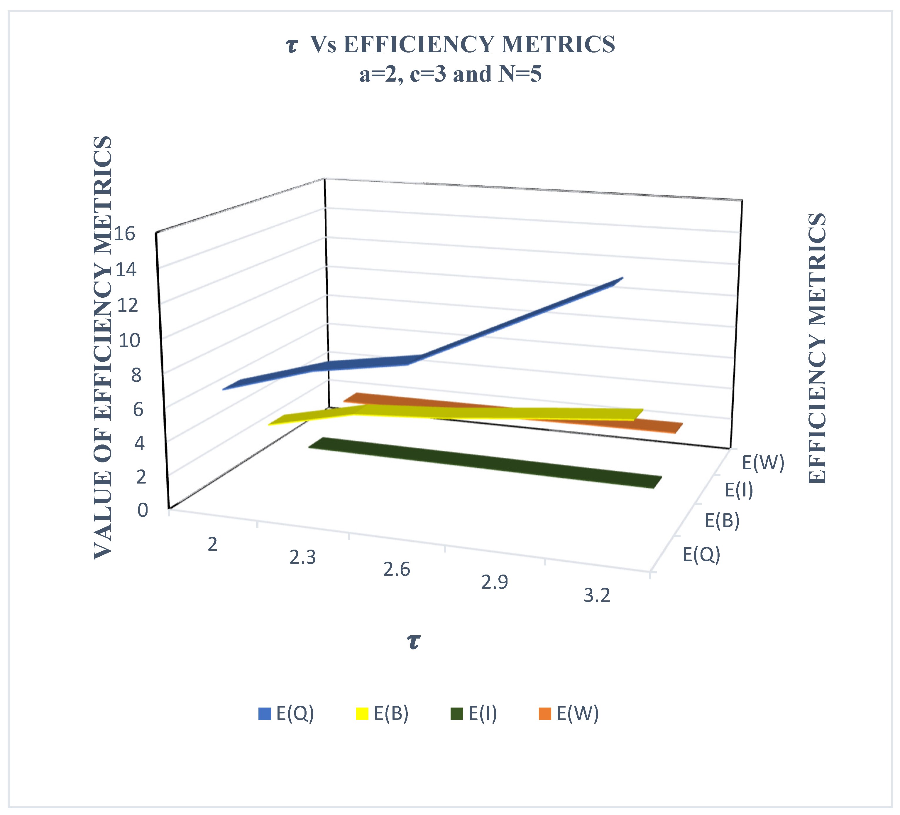
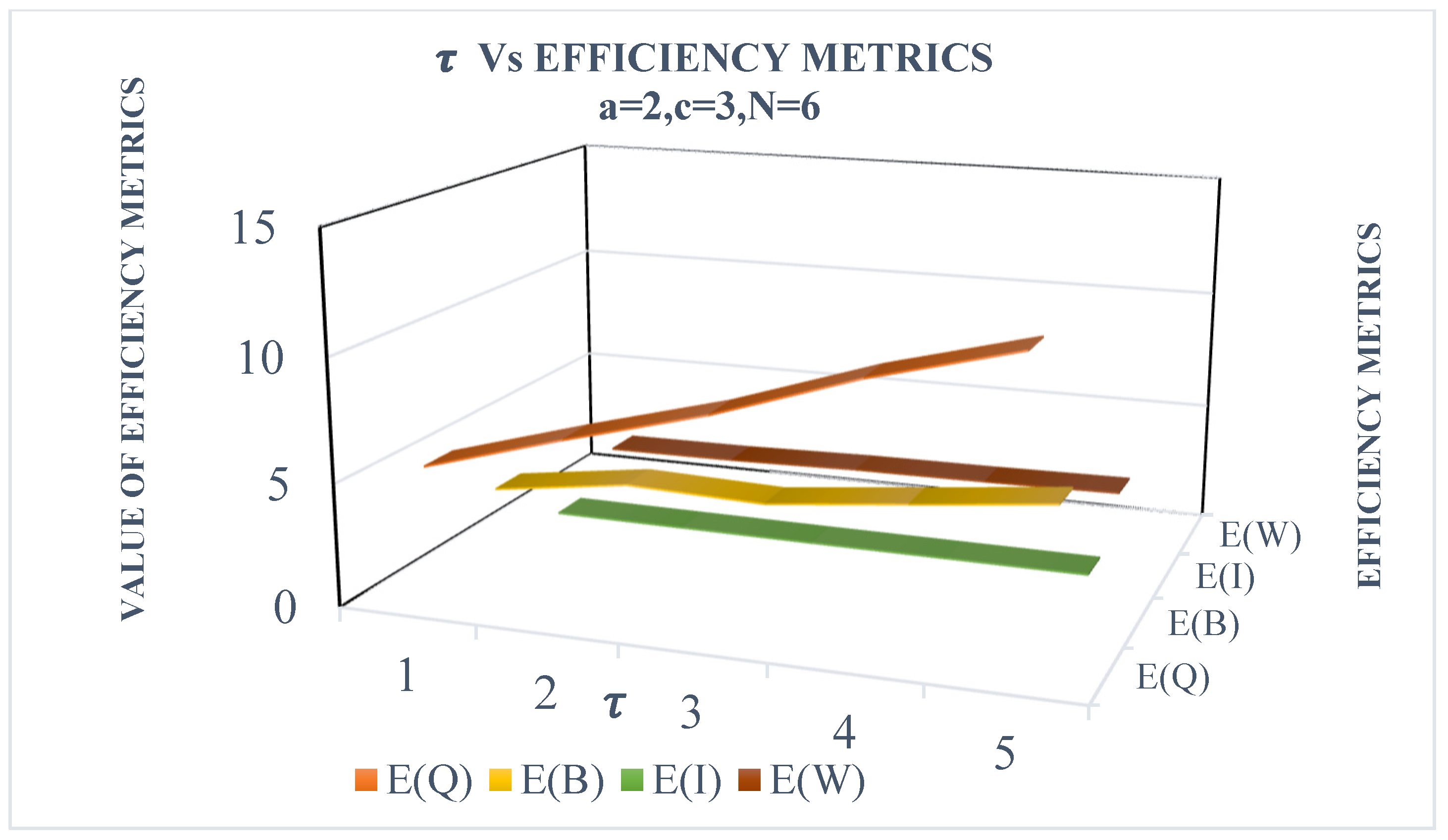
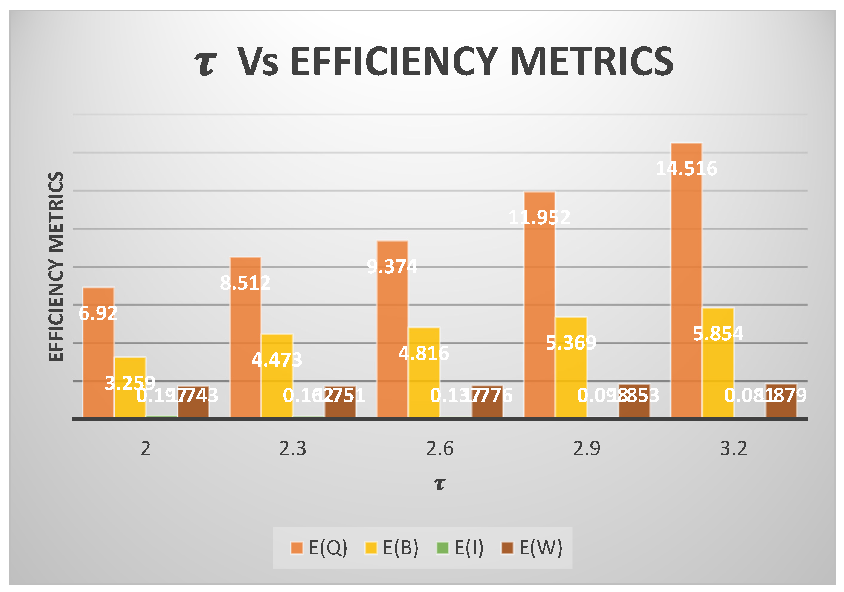
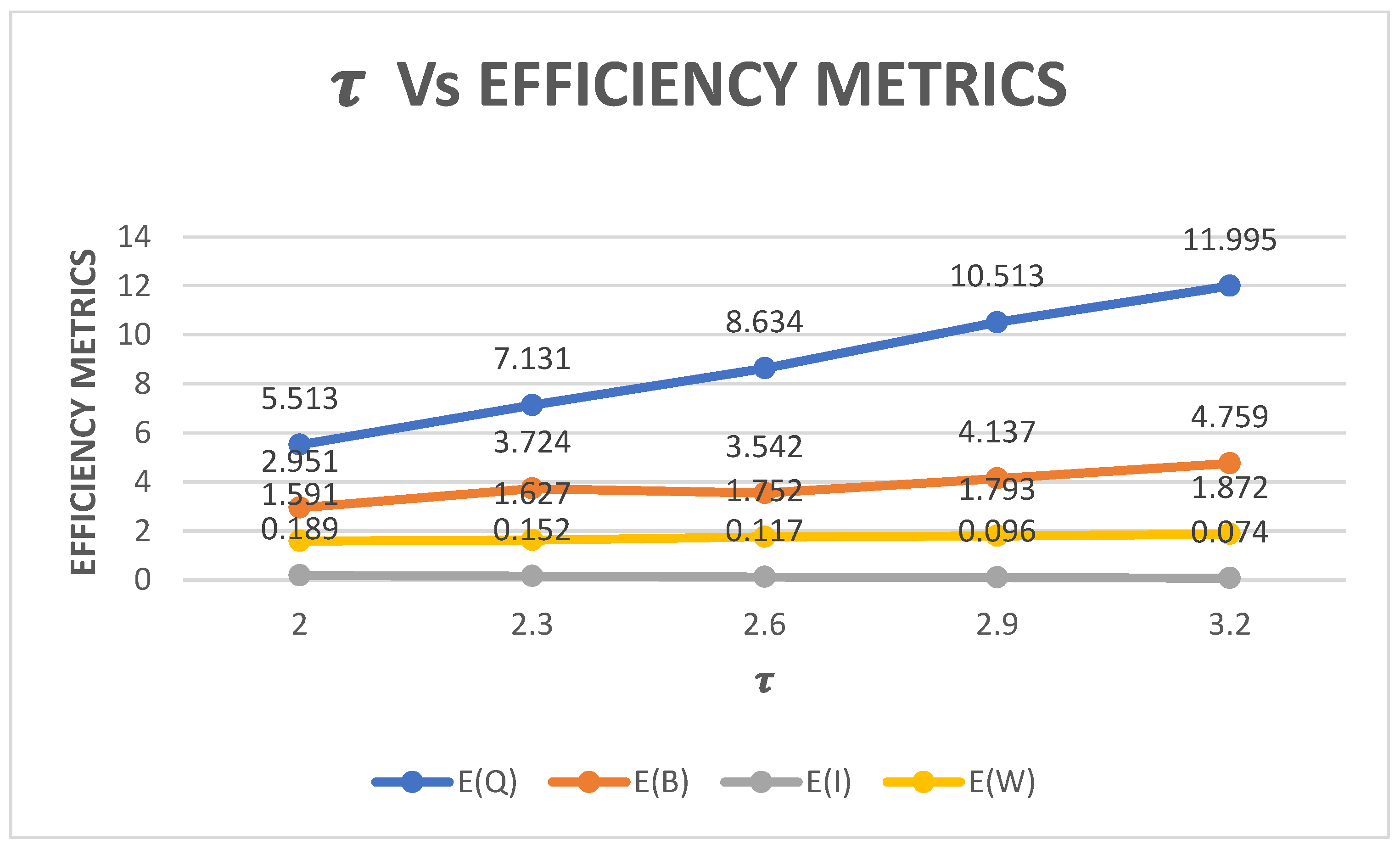
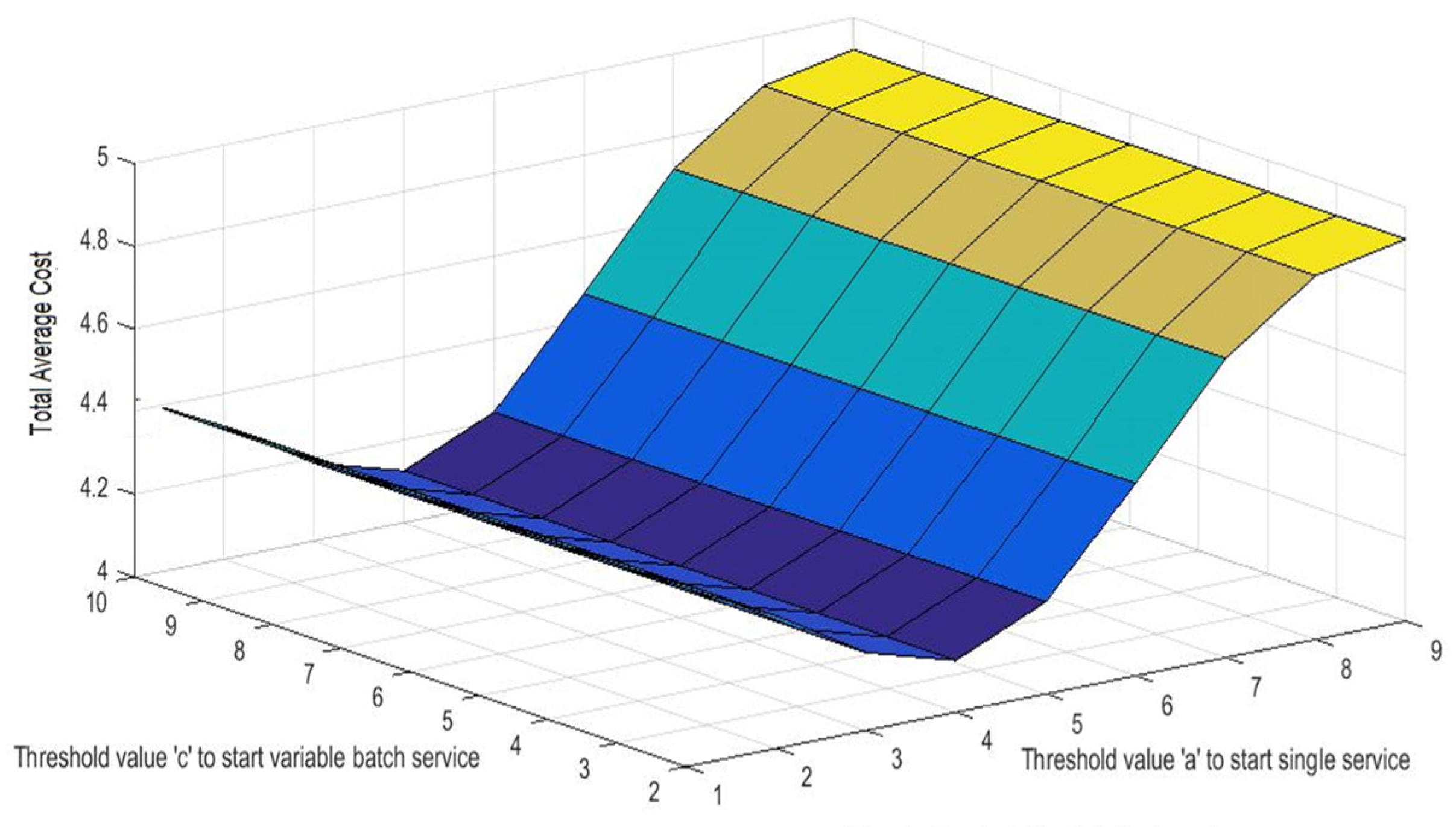
Effects of different efficiency metrics for a fixed threshold value are given in

Table 5. $\tau$ vs. efficiency metrics.

a = 3, c = 3 and N = 5					a = 3, c = 4, N = 6
$\mathit{\tau }$	${\mathit{L}}_{\mathit{q}\mathit{u}\mathit{e}\mathit{u}\mathit{e}}$	${\mathit{L}}_{\mathit{b}\mathit{u}\mathit{s}\mathit{y}}$	${\mathit{L}}_{\mathit{i}\mathit{d}\mathit{l}\mathit{e}}$	${\mathit{W}}_{\mathit{q}\mathit{u}\mathit{e}\mathit{u}\mathit{e}}$	${\mathit{L}}_{\mathit{q}\mathit{u}\mathit{e}\mathit{u}\mathit{e}}$	${\mathit{L}}_{\mathit{b}\mathit{u}\mathit{s}\mathit{y}}$	${\mathit{L}}_{\mathit{i}\mathit{d}\mathit{l}\mathit{e}}$	${\mathit{W}}_{\mathit{q}\mathit{u}\mathit{e}\mathit{u}\mathit{e}}$
2.0	6.920	3.259	0.197	1.743	5.513	2.951	0.189	1.591
2.3	8.512	4.473	0.162	1.751	7.131	3.724	0.152	1.627
2.6	9.374	4.816	0.137	1.776	8.634	3.542	0.117	1.752
2.9	11.952	5.369	0.098	1.853	10.513	4.137	0.096	1.793
3.2	14.516	5.854	0.081	1.879	11.995	4.759	0.074	1.872

and Figure 2, Figure 3, Figure 4 and Figure 5 with the following assumptions: a = 2, c = 2, N = 5 and a = 2, c = 3, N = 6. It is clear that if $\tau$ increases the mean queue length, the average waiting time in the queue and the average duration of the busy period will increase, whereas the average duration of the idle period will decrease. All the outcomes were attained using MATLAB software. From Figure 6, it is observed that the results help to minimize the aggregate mean cost of the system by fixing the threshold values.

4.2. Optimal Cost

This section presents a numerical example to demonstrate how manufacturing pharmaceutical tablets can utilize the obtained results. By setting appropriate threshold values, the goal is to minimize the system’s aggregate mean cost effectively. The effects of threshold values ‘a’ and ‘c’ on the aggregate mean cost are presented in

Table 6. Initial value to start vs. aggregate mean cost for $b=7$ and $N=15$.

Threshold Value ‘$c$’ to Start Batch Service
Threshold value ‘$a$’ to start single service		c	2	3	4	5	6
	a		Aggregate mean cost
	1		5.342	5.126	5.563	5.645	5.763
	2			5.342	5.482	5.544	5.656
	3				5.154	5.334	5.431
	4					5.112	5.231
	5						4.984

Minimum aggregate mean cost occurs when a = 5, c = 6 for b = 7.

,

Table 7. Initial value to start versus aggregate mean cost for $b=9$ and $N=17$.

	Threshold Value $\mathrm{‘}c\mathrm{’}$ to Start Batch Service
Threshold value ‘$a$’ to start single service		c	2	3	4	5	6	7	8
	a		Aggregate mean cost
	1		4.321	4.202	4.116	4.783	4.472	4.743	5.135
	2			4.126	3.998	4.553	4.372	4.541	4.884
	3				2.971	4.445	4.122	4.432	4.683
	4					4.323	4.032	4.332	4.565
	5						4.011	4.211	4.345
	6							3.971	4.282
	7								4.154

Minimum aggregate mean cost occurs when a = 6, c = 7 for b = 9.

and

Table 8. Initial value to start versus total average cost for b = 11 and $N=20$.

	Threshold Value $\mathrm{‘}c\mathrm{’}$ to Start Batch Service
$\mathrm{Threshold} \mathrm{value} ‘a$’ to start single service		c	2	3	4	5	6	7	8	9	10
	a		Aggregate mean cost
	1		4.431	4.321	4.188	4.125	4.223	4.465	4.723	4.879	4.923
	2			4.112	4.09.	2.833	4.112	4.332	4.632	4.776	4.654
	3				4.012	2.567	4.132	4.221	4.544	4.655	4.235
	4					2.643	4.155	4.112	4.445	4.521	4.112
	5						4.166	4.092	4.321	4.432	4.02
	6							4.093	4.232	4.232	3.987
	7								4.012	4.112	3.722
	8									4.022	3.654
	9										3.442

Minimum aggregate mean cost occurs when a = 7, c = 8 for b = 11.

with the following parameters: b = 7, N = 15, b = 9, N = 17 and b = 11, N = 20. From the above tables, it can be seen that the system is capable of performing single service and bulk service with maximum capacity: b = 7 or b = 9 or b = 11. Therefore, the management of the system has to fix the threshold values as a = 5, c = 6 and b = 7, a = 6, c = 7, and b = 9 and a = 7, c = 8, and b = 11, respectively, to minimize the aggregate mean cost.

5. Conclusions

This study investigated bulk queueing systems that incorporate various service modes and server vacations. The model is distinctive in that it introduces three separate service modes for a single server within a bulk arrival and batch service queueing system. Using the supplementary variable technique, the probability-generating function for the queue size at any given time is derived. A range of performance metrics is presented, along with numerical examples. Furthermore, an optimal cost analysis is performed to minimize the system’s aggregate mean cost by establishing threshold values for the different service modes.

In the future, this model can be extended with multiple vacations and vacation interruptions with the intention on the basis of the effective utilization of idle time of the server. An attempt can be made to study the queueing model in a fuzzy environment; that is, fuzzy numbers will be used as the parameters, such as arrival rate, service rate, and vacation rate, instead of using the probability distribution.

References

1. Shortle, J.F.; Thompson, J.M.; Gross, D.; Harris, C.M. Fundamentals of Queueing Theory; John Wiley & Sons: Hoboken, NJ, USA, 2018. [Google Scholar]
2. Takagi, H. Queueing Analysis: A Foundation of Performance Evaluation; Distributors for the U.S. and Canada, Elsevier Science Pub. Co.: New York, NY, USA; Amsterdam/North-Holland, The Netherland, 1991. [Google Scholar]
3. Tian, N.; Zhang, Z.G. Vacation Queueing Models Theory and Applications; Springer US (International Series in Operations Research & Management Science): Boston, MA, USA, 2006. [Google Scholar] [CrossRef]
4. Doshi, B.T. Queueing systems with vacations—A survey. Queueing Syst. 1986, 1, 29–66. [Google Scholar] [CrossRef]
5. Lee, H.W.; Lee, S.S.; Park, J.O.; Chae, K.C. Analysis of the Mx/G/1 queue by N-policy and multiple vacations. J. Appl. Probab. 1994, 31, 476–496. [Google Scholar] [CrossRef]
6. Neuts, M.F. A General Class of Bulk Queues with Poisson Input. Ann. Math. Stat. 1967, 38, 759–770. [Google Scholar] [CrossRef]
7. Haridass, M.; Arumuganathan, R. Analysis of a MX/G(a,b)/1 queueing system with vacation interruption. RAIRO Oper. Res. 2012, 46, 305–334. [Google Scholar] [CrossRef]
8. Wu, W.; Tang, Y.; Yu, M. Analysis of an M/G/1 queue with N-policy, single vacation, unreliable service station and replaceable repair facility. OPSEARCH 2015, 52, 670–691. [Google Scholar] [CrossRef]
9. Niranjan, S.P.; Indhira, K. A Review on Classical Bulk Arrival and Batch Service Queueing Model. Int. J. Pure Appl. Math. 2016, 106, 45–51. [Google Scholar]
10. Nobel, R.D.; Tijms, H.C. Optimal control for an MX/G/1 queue with two service modes. Eur. J. Oper. Res. 1999, 113, 610–619. [Google Scholar] [CrossRef]
11. Singh, C.; Jain, M.; Kaur, S. Performance analysis of bulk arrival queue with balking, optional service, delayed repair and multi-phase repair. Ain Shams Eng. J. 2017, 9, 2067–2077. [Google Scholar] [CrossRef]
12. Ayyappan, G.; Deepa, T. Analysis of batch arrival bulk service queue with multiple vacation closedown essential and optional repair. Appl. Appl. Math. 2018, 13, 2. [Google Scholar]
13. Niranjan, S.P.; Indhira, K.; Chandrasekaran, V.M. Analysis of bulk arrival queueing system with batch size dependent service and working vacation. In AIP Conference Proceedings; AIP Publishing: Melville, NY, USA, 2018. [Google Scholar] [CrossRef]
14. Ayyappan, G.; Karpagam, S. Analysis of a bulk queue with unreliable server, immediate feedback, N-policy, Bernoulli schedule multiple vacation and stand-by server. Ain Shams Eng. J. 2019, 10, 873–880. [Google Scholar] [CrossRef]
15. Niranjan, S.P. Managerial decision analysis of bulk arrival queuing system with state dependent breakdown and vacation. Int. J. Adv. Oper. Manag. 2020, 12, 351–376. [Google Scholar] [CrossRef]
16. Niranjan, S.P.; Chandrasekaran, V.M.; Indhira, K. Phase dependent breakdown in bulk arrival queueing system with vacation break-off. Int. J. Data Anal. Tech. Strateg. 2020, 12, 127–154. [Google Scholar] [CrossRef]
17. Betsch, S.; Ebner, B. Fixed point characterizations of continuous univariate probability distributions and their applications. Ann. Inst. Stat. Math. 2021, 73, 31–59. [Google Scholar] [CrossRef]
18. Jeganathan, K.; Selvakumar, S.; Anbazhagan, N.; Amutha, S.; Hammachukiattikul, P. Stochastic modeling on M/M/1/N inventory system with queue-dependent service rate and retrial facility. AIMS Math. 2021, 6, 7386–7420. [Google Scholar] [CrossRef]
19. Chaves, C.; Gosavi, A. On general multi-server queues with non-poisson arrivals and medium traffic: A new approximation and a COVID-19 ventilator case study. Oper. Res. 2022, 22, 5205–5229. [Google Scholar] [CrossRef]
20. Kumar, V.; Upadhye, N.S. On first-come, first-served queues with three classes of impatient customers. Int. J. Adv. Eng. Sci. Appl. Math. 2021, 13, 368–382. [Google Scholar] [CrossRef]
21. Kim, J.J.; Down, D.G.; Chaudhry, M.; Banik, A.D. Difference Equations Approach for Multi-Server Queueing Models with Removable Servers. Methodol. Comput. Appl. Probab. 2022, 24, 1297–1321. [Google Scholar] [CrossRef]
22. Wei, Q.; Chen, X. Continuous-Time Markov Decision Processes Under the Risk-Sensitive First Passage Discounted Cost Criterion. J. Optim. Theory Appl. 2023, 197, 309–333. [Google Scholar] [CrossRef]
23. Shen, G.; Li, Q.; Shi, W.; Jiang, Y.; Zhang, P.; Gu, L.; Xu, M. Modeling and optimization of the data plane in the SDN-based DCN by queuing theory. J. Netw. Comput. Appl. 2022, 207, 103481. [Google Scholar] [CrossRef]
24. Shiripour, S.; Hematian, M.; Mahdavi-Amiri, N. A robust optimization model for dynamic virtual hub location problem under uncertainty using an M/M/C/K queuing model: Two metaheuristic algorithms. Oper. Res. 2023, 23, 40. [Google Scholar] [CrossRef]
25. Chakravarthy, S.R.; Shruti Rumyantsev, A. Analysis of a Queueing Model with Batch Markovian Arrival Process and General Distribution for Group Clearance. Methodol. Comput. Appl. Probab. 2021, 23, 1551–1579. [Google Scholar] [CrossRef] [PubMed]
26. Wang, W.; Ji, Y.; Zhao, Z.; Yin, H. Simulation Optimization of Station-Level Control of Large-Scale Passenger Flow Based on Queueing Network and Surrogate Model. Sustainability 2024, 16, 7502. [Google Scholar] [CrossRef]
27. Wang, W.; Liu, Y.; Fan, X.; Zhang, Z. Optimization of Charging Station Capacity Based on Energy Storage Scheduling and Bi-Level Planning Model. World Electr. Veh. J. 2024, 15, 327. [Google Scholar] [CrossRef]
28. Huang, R.; Xie, X.; Guo, Q. Multi-Queue-Based Offloading Strategy for Deep Reinforcement Learning Tasks. Electronics 2024, 13, 2307. [Google Scholar] [CrossRef]
29. CK, D.M.; Selvamuthu, D.; Kalita, P. Energy Efficiency in a Base Station of 5G Cellular Networks using M/G/1 Queue with Multiple Sleeps and N-Policy. Methodol. Comput. Appl. Probab. 2023, 25, 48. [Google Scholar] [CrossRef]
30. Niranjan, S.P.; Latha, S.D. Analyzing the Two-Phase Heterogeneous and Batch Service Queuing System with Breakdown in Two-Phases, Feedback, and Vacation. Baghdad Sci. J. 2024, 21, 2701. [Google Scholar] [CrossRef]
Figure 1. Model description. Q-Queue length.
Mathematics 12 03535 g001
Figure 2. τ vs. efficiency metrics. Here E ( Q ) = L q u e u e ,   E ( B ) = L b u s y ,   E ( I ) = L i d l e , E(W) = W q u e u e .
Mathematics 12 03535 g002
Figure 3. τ vs. efficiency metrics. Here, E ( Q ) = L q u e u e ,   E ( B ) = L b u s y ,   E ( I ) = L i d l e , E(W) = W q u e u e .
Mathematics 12 03535 g003
Figure 4. τ vs. efficiency metrics. a = 2, c = 3, N = 5. Here, E ( Q ) = L q u e u e ,   E ( B ) = L b u s y ,   E ( I ) = L i d l e , E(W) = W q u e u e .
Mathematics 12 03535 g004
Figure 5. τ vs. efficiency metrics. a = 3, c = 4, N = 6. Here, E ( Q ) = L q u e u e ,   E ( B ) = L b u s y ,   E ( I ) = L i d l e , E(W) = W q u e u e .
Mathematics 12 03535 g005
Figure 6. Initial value to start versus aggregate mean cost for N = 20 . Minimum aggregate mean cost occurs when a = 7, c = 8 for b = 11.
Mathematics 12 03535 g006