Abstract
The total least squares method has a broad applicability in many fields. It is also useful in fuzzy data analysis. In this paper, we study the method of total least squares for fuzzy variables. The regression parameters are considered to be crisp. First, we find a formula for the distance between an arbitrary pair of triangular fuzzy numbers and the set described by the regression relation. Second, we develop a new approach to total least squares for data that are modeled as symmetric triangular fuzzy numbers. To illustrate the theoretical results obtained in the paper, some numerical examples are presented.
Keywords:
regression; total least squares; fuzzy number; fuzzy regression; triangular fuzzy number; symmetric triangular fuzzy number MSC:
62J05; 90C70
1. Introduction
The least squares method (LS) and the total least squares method (TLS) have been widely discussed in many papers. Various approaches have been developed, and numerous practical applications have been discovered. As the study of fuzzy regression has advanced, the use of LS and TLS methods together with fuzzy numbers has been discussed. In this article, we focus on the TLS technique. In the following lines, we mention some results obtained in various works. These results are part of a broader framework within which this article can also be included.
Some exponential fitting models and TLS techniques with applications in a fairly large number of environmental problems, such as watershed rainfall-runoff modeling and forecasting water consumption in certain regions of Earth, are shown in [1]. In [2] are presented some generalizations of TLS that are mainly based on the addition of constraints and the use of regularization and weighted norms. There are books that focus on the TLS procedure [3,4]. These books bring forward discussions ranging from basic concepts to numerous generalizations and applications. In [5], an algorithm for the TLS method is presented, and the relation between LS and TLS is discussed. In [6], some orthogonal regression approaches are presented. Moreover, these approaches are compared from theoretical and practical points of view. The utility of orthogonal regression for the study of seismic hazard is emphasized. In [7], the generalization of the TLS method is discussed, and its importance in various domains such as system theory and signal processing is highlighted. In [8], three methods of regression, namely Chi-square regression, general orthogonal regression and weighted total least squares, are used for the topic of earthquake magnitude conversion. In [9], a new algorithm that is based on a regularized loss function is employed to deal with the orthogonal regression problem. In [10], orthogonal regression is discussed in relation to eruption data of a geyser. In [11], a MATLAB 7.0 (R14) routine for TLS is used to describe the economies of a group of four East European countries. In [12], a MATLAB 7.11 (R2010b) toolbox for problems related to TLS is presented. In [13], real estate prices are studied, and it is proved that TLS is better than ordinary least squares when using the Hedonic Price Model. In [14], there is given a fuzzy regression model based on least squares, where independent variables are crisp, and the response variables are L-R fuzzy numbers. The L-R representation of a fuzzy number is discussed in [15]. To analyze environmental effects in the process of modeling complex systems from the field of systems science, [16] discusses some fuzzy regression models that use, among other types of fuzzy numbers, symmetric triangular fuzzy numbers. In [17], numerous papers from the field of fuzzy regression analysis are systematically discussed. In [18], triangular fuzzy numbers are used to study some characteristics of logistics centers. In [19], a neuro-fuzzy inference system is used in a fuzzy regression model with trapezoidal fuzzy outputs. In [20], fuzzy regression is employed to study technological developments. In [21], there is presented a comparison between ordinary least squares and fuzzy least squares in the framework of a simulation experiment regarding pharmacokinetic parameters. Taking into account the uncertainty theory [22], two linear regression methods are discussed in [23]: an uncertain total least squares estimation and an uncertain robust total least squares estimation. In [23], work with uncertain variables is performed considering the expected value of an uncertain variable [22]. In [24], orthogonal least squares is used to develop an orthogonal least squares learning algorithm. In [25], the TLS method is improved by considering constrained TLS parameter optimization. In [26], an orthogonal least squares-based fuzzy filter with a small computational load is proposed. It is used in analysis of lung sounds. The work in this field is continued in [27]. Paper [28] discusses methods that use deep learning and regression in fuzzy logic systems, focusing on accuracy and interpretability. In [29,30], quadratic programming is considered for use in fuzzy regression models. In [31], various approaches to fuzzy least squares and fuzzy orthogonal least squares are investigated. In [32,33], fuzzy regression is used to study some aquifer systems. In [32], a relation between some drought indices and the observed water table in two geographical areas is established. In [33], fuzzy regression is employed to deal with uncertainty when monitoring some biological quality elements in six Greek lakes. TLS regression was also proved useful in Geodesy [34,35]. In [34], an errors-in-observations model is used with a TLS algorithm. In [36], fuzzy regression is considered for real estate price prediction. In [37], the orthogonal least squares method is modified, and it is applied to a fault detection depollution problem. In [38], there is developed a regression model that can be used for triangular and other types of fuzzy numbers. A fuzzy least squares model is given in [39]. In [39], the least squares technique is used for general fuzzy data, and an application for data modeled as triangular fuzzy numbers is also presented.
This paper is organized as follows. Some concepts and formulas from previous works are presented in Section 2. We consider the approach from [39] regarding the definition of the distance between two fuzzy numbers. This definition uses the parameterization of a fuzzy number [40]. In Section 3 we analyze the distances from a certain triangular fuzzy number to each element of a particular set of triangular fuzzy numbers, and we identify the element from the set for which the smallest distance is obtained. This smallest distance is regarded as the distance between that certain triangular fuzzy number and the considered set. Section 4 contains the main theoretical results, and it is divided into several subsections. In Section 4.1, we give a method for calculating the sum of squared distances from some triangular fuzzy numbers to a particular set of triangular fuzzy numbers. This particular set of fuzzy numbers, which we can call the fuzzy regression set, replaces the regression line that appears when only real numbers are used. In Section 4.2, we consider the special case of symmetric triangular fuzzy numbers. This subsection contains theoretical results regarding the parameters that define the fuzzy regression set. The possible cases that can be encountered in applications are systematically discussed in Section 4.3. In Section 4.4, the steps of the algorithm are presented. To illustrate the viability of the method, some numerical examples are provided in Section 5. Some comments are given in Section 6. Section 7 contains the conclusions.
2. Preliminaries—Materials and Methods
We consider the definition of a fuzzy number as given in [39]. We denote a triangular fuzzy number by , where is the real value at which the membership function takes the value 1, is the left spread, and is the right spread. We have and . The membership function of is
For , the -cut is , where and [39,40]. If , then we obtain a symmetric triangular fuzzy number [16], which can be denoted by .
Let be a pair of triangular fuzzy numbers, where , .
We consider the set , where are triangular fuzzy numbers and , . The operations involving fuzzy numbers follow the general rules discussed in [15,39,40]. The two possible situations for the sign of will be treated separately, because this sign influences the form of the elements belonging to the set . We use the metric that is considered in [39]. We have [39]
and
3. On Distance from a Triangular Fuzzy Number to a Certain Set of Fuzzy Numbers
Proposition 1.
If , and , then there exists a unique element such that
for all .
Moreover, we have
where
Proof.
The proof is given in Appendix A. □
Proposition 2.
If , and , then there exists a unique element such that
for all .
Moreover, we have
where
Proof.
The proof is given in Appendix A. □
If is a symmetric triangular fuzzy number, then its membership function is
In this case, has the -cut , where , and .
In Proposition 1, if is a pair of symmetric triangular fuzzy numbers, we obtain
In Proposition 2, if is a pair of symmetric triangular fuzzy numbers, we obtain
4. Total Least Squares for Symmetric Triangular Fuzzy Numbers
4.1. Preliminary Results
Let , , be pairs of triangular fuzzy numbers, where and . For all , we have
and
Let us recall that , where are triangular fuzzy numbers and . We consider the sum
For every , , the pair is given by Proposition 1, and the pair is given by Proposition 2. The following two propositions give formulas for .
Proposition 3.
Consider the set , where are triangular fuzzy numbers and . If and , for all , then
Proof.
The proof is given in Appendix A. □
Proposition 4.
Consider the set , where are triangular fuzzy numbers and . If and , for all , then
Proof.
The proof is given in Appendix A. □
4.2. Theoretical Results on the Total Least Squares for Symmetric Triangular Fuzzy Numbers
Let , , be pairs of symmetric triangular fuzzy numbers, where and .
For all , we have
and
We must find the parameters and , which define the set , such that
is minimized. In other words, the optimization problem to be solved is
Proposition 5.
If and , , for all , then
Proof.
Taking into account the equalities and , for all , the result follows from Proposition 3. □
Proposition 6.
If and , , for all , then
Proof.
Taking into account the equalities and , for all , the result follows from Proposition 4. □
Proposition 7.
Let , , , be pairs of symmetric triangular fuzzy numbers, where and . It is assumed that the relation
is true, where
The inequality
is a necessary and sufficient condition for the existence and unicity of a pair such that
Moreover, the following relations hold:
Proof.
According to Proposition 5, if , we have
We obtain
Further, we can obtain
Thus we can write
where
We also obtain
Using (2), we can write
Using (1), we obtain
Using (5), we obtain
We can conclude that
From (5), we obtain
Consider the system
and the Hessian matrix
Using relation (5), the equation
gives
Thus, we successively obtain
and
We obtain
and
Using (11), we also have
and
Using relation (1), the equation
becomes
Thus,
Using (16) and (10), we can write
which is equivalent to
Using (12) and (13), from (17) we obtain
which gives
Relation (18) can be written as
where
The discriminant of Equation (19) is
which is a nonnegative real number.
Equation (19) has at least one real solution, and can be obtained from (11). Let be a generic solution, from of system (9).
Using Formula (2) and the fact that verifies the first equation of system (9), we obtain
Using (6) and (22), we obtain
The pair fulfills relations (10)–(15), because it is a solution of system (9). Using (3) and (14), we obtain
Using (4) and (15), we obtain
Using (23)–(25), we obtain
Thus, we can write
where
Taking into account (21), (27) and (28), we remark that
Using (19) and (29), we obtain
Thus, we have
and
We obtain
Finally, taking into account (26), we have
Using (10), which is verified by , and (7), we obtain
From (8), we have
From (31)–(33) the Hessian matrix becomes
We have
Since verifies Equation (19), we can write
Thus, and are both strictly positive if and only if and have the same sign.
If , Equation (19) has two distinct solutions, namely
from which only one is strictly positive.
If , let be the unique strictly positive solution of (19), namely
Thus,
where is obtained from (11) as
If , Equation (19) has the solution , which is not in . □
Proposition 8.
Let , , , be pairs of symmetric triangular fuzzy numbers, where and . It is assumed that the relation
is true, where
The inequality
is a necessary and sufficient condition for the existence and unicity of a pair such that
Moreover, the following relations hold:
Proof.
According to Proposition 6, if , we have
We obtain
Further, we can obtain
Thus, we can write
where
We also obtain
Using (35), we can write
Using (34), we obtain
From (38), we obtain
We can conclude that
From (38), we obtain
Consider the system
and the Hessian matrix
Using relation (38), the equation
gives
Taking into account (10) and (43), note that using the same reasoning as in (11)–(15), we can write the following relations:
Using relation (34), the equation
becomes
Thus,
Using (49) and (43), we can write
which is equivalent to
Using (45) and (46), from (50) we obtain
which gives
Relation (51) can be written as
where
The discriminant of Equation (52) is
which is a nonnegative real number.
Equation (52) has at least one real solution, and can be obtained from (44). Let be a generic solution, from , of system (42).
Using Formula (35) and the fact that verifies the first equation of system (42), we obtain
Using (39) and (55), we obtain
The pair satisfies relations (43)–(48), because it is a solution of system (42). Using (36) and (47), we obtain
Using (37) and (48), we obtain
Using (56)–(58), we obtain
Thus, we can write
where
Taking into account (54), (60) and (61), we can remark that
Using (52) and (62), we obtain
Thus, we have
and
We obtain
Finally, taking into account (59), we have
Using (43), which is verified by and (40), we obtain
From (41), we have
From (64)–(66), the Hessian matrix becomes
We have
Since verifies Equation (52), we can write
Thus and are both strictly positive if and only if and have the same sign.
If , Equation (52) has two distinct solutions, namely
from which only one is strictly negative.
If , let be the unique strictly negative solution of (52), namely
Thus,
where is obtained from (44) as
If , Equation (52) has the solution , which is not in . □
Proposition 9.
The following relation holds:
Proof.
Using Formulas (20) and (53) from Proposition 7 and Proposition 8, respectively, we obtain
We obtain , since for all . □
Proposition 10.
If , then
where
Proof.
Using Proposition 5 together with relations (14) and (15), we obtain
□
Proposition 11.
If then
Proof.
Using Proposition 6 together with relations (47) and (48), we have
□
4.3. Concluding Theoretical Discussion
In this part of the article, we analyze the possibilities that arise when solving the optimization problem
which is stated at the beginning of Section 4.2.
In accordance with Proposition 9, the inequalities and cannot be simultaneously true. Moreover, and cannot be both equal to zero.
By considering Propositions 7–11, a structured theoretical discussion will have to include certain cases that are split into subcases. The division into cases is related to while the possibilities for and are studied in subcases.
Case 1.
Consider the situation in which .
Subcase 1.1.
, .
According to relation (53) and Proposition 9, the inequalities and are simultaneously true if and only if
Using Propositions 7 and 8, we can conclude that is the solution for the optimization problem, where is obtained in Proposition 7.
Subcase 1.2.
, .
The relations and are simultaneously true if and only if
Taking again into account Propositions 7 and 8, the solution is .
Subcase 1.3.
,.
The inequalities and are simultaneously true if and only if
We consider the pairs and from Proposition 7 and Proposition 8, respectively.
The solution is when .
The solution is when .
If there exists a set of data such that , then both and can be taken as solutions.
Subcase 1.4.
,
The relations and are simultaneously true if and only if
Taking into account Propositions 7 and 8, the solution is .
Subcase 1.5.
, .
The inequalities and are simultaneously true if and only if
According to Propositions 7 and 8, the solution is .
Case 2.
Consider the situation in which .
Subcase 2.1.
, .
From relation
which is given in Proposition 7, we obtain
We have
From Proposition 10, we obtain
Since must be strictly negative, in Proposition 8 we retain the stationary point
Note that, in Proposition 8, the determinant is strictly negative.
From Proposition 11, we obtain
By using the inequalities and we can write
In conclusion, the solution for the optimization problem is , where
Subcase 2.2.
, .
As in Subcase 2.1, from Proposition 7 we have .
From Proposition 10, we obtain
If , , , from Proposition 11 we obtain
We have
and we can conclude that the solution is
Subcase 2.3.
,
As in Subcase 2.1, we obtain and
Using the formula
which is given in Proposition 8, we obtain .
We have
Using Proposition 11, we obtain
We have
If we obtain and the solution is
If , the solution is
If , we obtain .
Subcase 2.4.
,
As in Subcase 2.3, from Proposition 8 we obtain .
From Proposition 11, we have
If , from Proposition 10 we obtain
We have
The solution is
Subcase 2.5.
, .
From Proposition 8, we obtain .
We have
Using Proposition 7, we retain the stationary point . Note that, in Proposition 7, the determinant is strictly negative.
From Proposition 10, we have
We obtain
The solution is , where
4.4. The Final Form of the Algorithm
Consider the following formulas:
The results obtained in the paper can be summarized as follows.
- ;
- 1.1
- . The solution is .
- 1.2
- . The solution is .
- 1.3
- ;
- 1.3.1.
- . The solution is .
- 1.3.2.
- . The solutions are: , .
- 1.3.3.
- . The solution is .
- 1.4
- . The solution is .
- 1.5
- . The solution is .
- ;
- 2.1
- . The solution is .
- 2.2.
- . The solution is .
- 2.3.
- ;
- 2.3.1.
- . The solution is .
- 2.3.2.
- . The solutions are: , .
- 2.3.3.
- . The solution is .
- 2.4.
- . The solution is .
- 2.5.
- . The solution is .
5. Numerical Examples
In this section, we consider some numerical examples.
Example 1.
Let , , be pairs of symmetric triangular fuzzy numbers, where , , , , , . We organize some of the calculations in Table A1; see Appendix B. Using the formulas from Section 4.4, we obtain , , and . Therefore, we have , and , . This example fits in Subcase 1.1. The solution is . We can write the relation
Thus, we have
Moreover, we obtain .
Fuzzy numbers can be characterized using certain crisp values, one of which is the possibilistic mean value [41]. The possibilistic mean value of a symmetric triangular fuzzy number is ; see [41]. Therefore, for and , we have and , .
Various graphical representations are used in works that study fuzzy numbers. In [42], a pair of fuzzy interval numbers is described using a rectangle. In [43], a fuzzy number is represented by a line segment. More precisely, in [43] the output values of a regression model are triangular fuzzy numbers that are represented by vertical line segments. Graphical representations related to the topic of fuzzy regression can also be found in [44,45,46].
Instead of a rectangle, we use a schematic representation formed by two intersecting line segments. We consider an arbitrary pair , where , , .
In the plane , we choose a closed horizontal line segment and a closed vertical line segment, as follows. The horizontal line segment has the endpoints and . The vertical line segment has the endpoints and .
The pair can be represented by the geometric shape formed by these two segments. Notably, the horizontal line segment and the vertical line segment intersect at point .
In the plane , we consider the line
If , where , , then . On the other hand, there are pairs such that and .
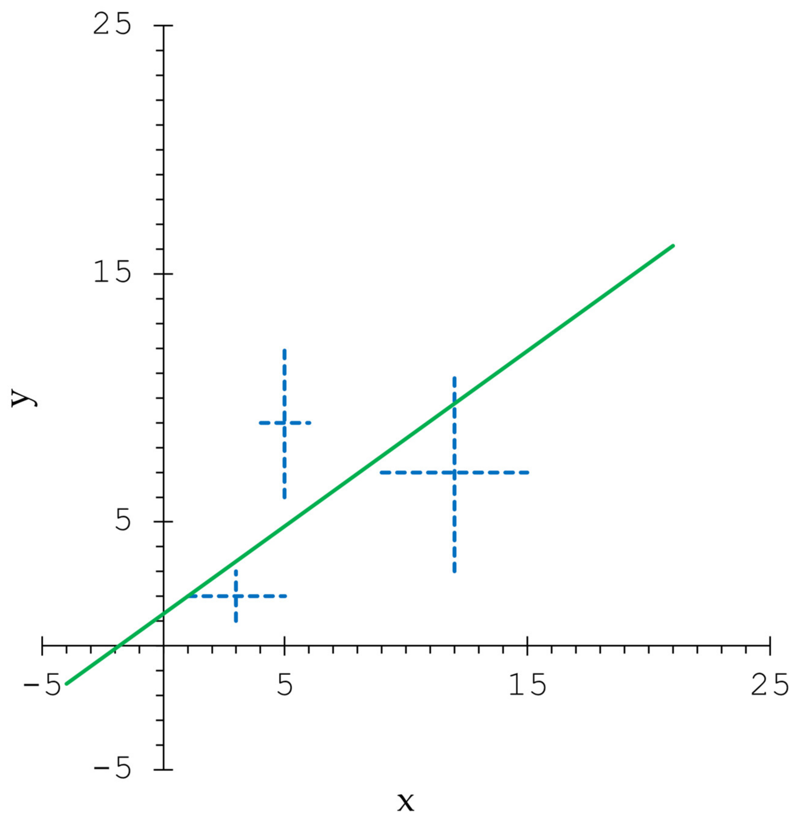
Figure 1 shows the line and the representations of the pairs , .
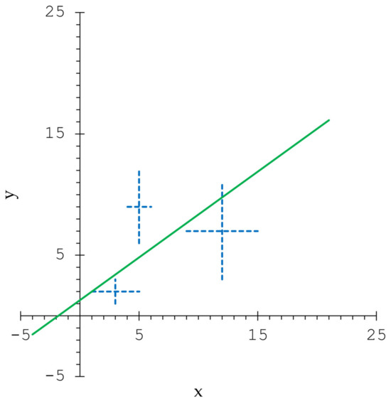
Figure 1.
The line and the representations of the pairs , .
In [11] it is emphasized that the regression relationship does not change even if the roles of the real variables are reversed. To see if this also happens in the case of symmetric triangular fuzzy variables, we consider the pairs , . We use again the results from Section 4.4. After reversing the roles of the fuzzy variables, it can be seen that and do not change their values, and only changes its sign. As in the case of regression for real numbers, we can obtain the relation
that is
or
Just like in the model for real data, the regression relation actually remains unchanged if the roles of the fuzzy variables are reversed. This kind of reasoning also works in the other theoretical subcases.
Example 2.
Let , , be pairs of symmetric triangular fuzzy numbers, where , , , , , , , . Using Table A2 from Appendix B, we have , , , . Therefore , and , . We obtain and . This example corresponds to Subcase 1.3. We obtain the solution .
Example 3.
Let , , be pairs of symmetric triangular fuzzy numbers, where , , , , , . Using Table A3 from Appendix B, we obtain , , , . Thus we have , and , . Further, we obtain . This example falls into Subcase 2.3, when the relation is true.
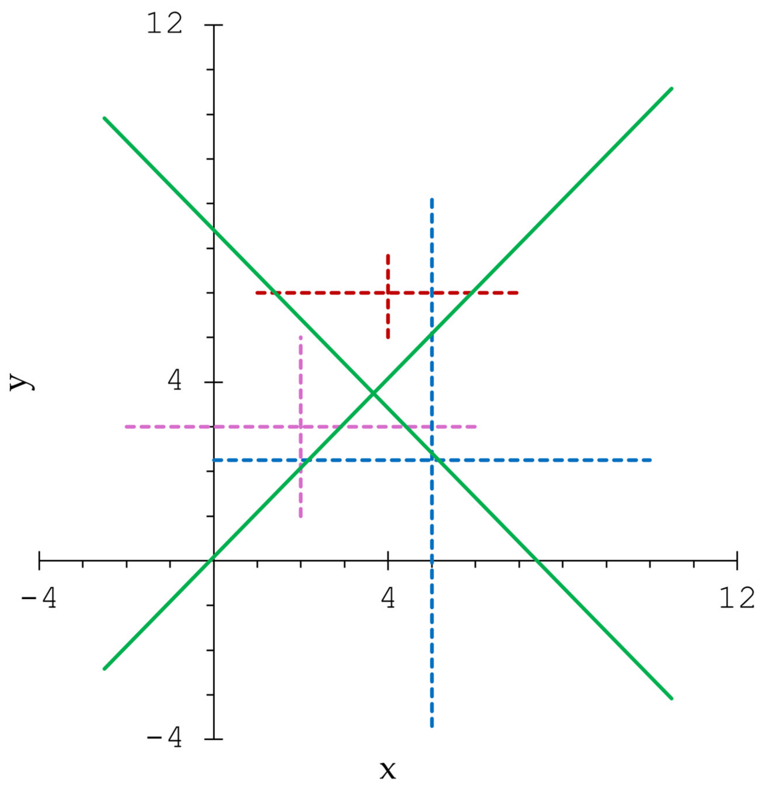
In the plane , we consider the lines
Figure 2 shows the lines , and the representations of the pairs , .
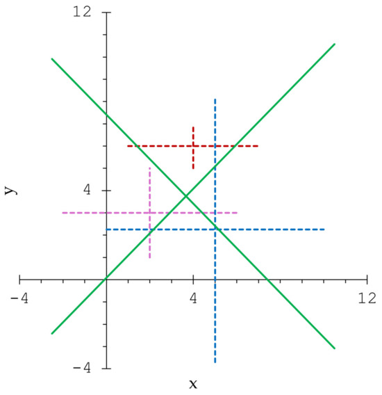
Figure 2.
The lines , and the representations of the pairs , .
Example 4.
Let , , be pairs of symmetric triangular fuzzy numbers, where , , , , , . Some intermediate calculations are given in Table A4, Appendix B. We obtain , , , . Therefore, we have , . This example illustrates Subcase 1.2. The solution is , for which .
6. Discussion
In the broad field of regression analysis, this paper falls into the area of methods that use fuzzy numbers. In this article, the method of total least squares is adapted for symmetric triangular fuzzy numbers. Triangular fuzzy numbers are often used in the literature. Moreover, if is the -cut of a triangular fuzzy number, then the functions and are defined on the compact interval and have certain properties that are highlighted in [39]. In the regression model for real numbers, the regression relationship does not change, even if the roles of the variables are reversed [11,47]. We remark that this phenomenon also occurs in the case of the method for fuzzy data: the same regression relationship is obtained regardless of whether the data , , or the data , , are considered. So, from this point of view, the results obtained in this paper are consistent with results from previous works.
In [39], the least squares method for fuzzy data is discussed. Considering what was discussed there, in this article the total least squares method for symmetric triangular fuzzy variables is approached. At the same time, this paper finds its place next to other works, such as [23,25,37], which study the use of regression in a framework marked by uncertainty.
7. Conclusions
The total least squares algorithm is a useful tool in the field of regression. In this paper, the total least squares method is used for an optimization model in which the data are modeled as symmetric triangular fuzzy numbers. In this way, the scope of the total least squares algorithm is widened from applications that use real data to applications that take into account the uncertainty described by fuzzy numbers. This paper contains general theoretical results, discussions on some particular cases and the systematic presentation of the steps of the final algorithm, and in this way it tries to offer a comprehensive work on the considered topic. To test the theoretical results, some numerical examples are discussed.
Author Contributions
Conceptualization, M.G. and C.-C.P.; methodology, M.G. and C.-C.P.; writing—original draft preparation, M.G. and C.-C.P. All authors have read and agreed to the published version of the manuscript.
Funding
This work was supported by the project “Societal and Economic Resilience within multi-hazards environment in Romania” funded by European Union—Nextgeneration EU and Romanian Government, under National Recovery and Resilience Plan for Romania, contract no. 760050/23.05.2023.
Data Availability Statement
The data used in the numerical examples are included in this work.
Acknowledgments
The authors express their gratitude to the support by the project “Societal and Economic Resilience within multi-hazards environment in Romania” funded by European Union—Nextgeneration EU and Romanian Government, under National Recovery and Resilience Plan for Romania, contract no.760050/23.05.2023.
Conflicts of Interest
The authors declare no conflicts of interest.
Appendix A. Proofs of Propositions 1–4
Proof of Proposition 1.
We have
We have
where
We consider the following system of equations:
We have
and
System (A1) can be written as
The determinant of the coefficient matrix of system (A2) is
System (A2) has a unique solution because .
For the ease of the calculus, we make the following notations:
The column of free terms from system (A2) is
We have
and
The unique solution of system (A2) is
Taking into account that and , we obtain .
We have
Thus, for the function , the Hessian matrix has the form
We obtain
We conclude that is the unique minimum point of the function . □
Proof of Proposition 2.
We have
We can write
We consider the following system:
We have
and
System (A3) can be written as
The determinant of the coefficient matrix of system (A4) is
System (A4) has a unique solution because .
For the ease of the calculus, we make the following notations:
The column of free terms from system (A4) is
Analogously to Proposition 1, we obtain the unique solution of system (A4):
Taking into account that and , we can write .
We have
The Hessian matrix of the function has the same form as the Hessian of the function from Proposition 1. Thus, is the unique minimum point of the function . □
Proof of Proposition 3.
Using Proposition 1, we obtain
where
We have
We obtain
Since
we obtain
Since
we obtain
Since
we obtain
We also have
We can conclude that
□
Proof of Proposition 4.
Considering Proposition 2, we have
where
Performing calculations similar to those in Proposition 3, we obtain
We also have
We obtain
Since
we obtain
Since
we obtain
Since
we obtain
We also have
We can conclude that
□
Appendix B. Intermediate Calculations for Examples 1–4

Table A1.
Intermediate calculations for example 1.
Table A1.
Intermediate calculations for example 1.
| 1 | 3 | 2 | 2 | 1 | 6 | 2 | 9 | 4 | 4 | 1 |
| 2 | 5 | 1 | 9 | 3 | 45 | 3 | 25 | 81 | 1 | 9 |
| 3 | 12 | 3 | 7 | 4 | 84 | 12 | 144 | 49 | 9 | 16 |
| Sum | 20 | 6 | 18 | 8 | 135 | 17 | 178 | 134 | 14 | 26 |
Table A2.
Intermediate calculations for example 2.
Table A2.
Intermediate calculations for example 2.
| 1 | 5 | 3 | 3 | 1 | 15 | 3 | 25 | 9 | 9 | 1 |
| 2 | 10 | 25 | 12 | 8 | 120 | 200 | 100 | 144 | 625 | 64 |
| 3 | 14 | 8 | 13 | 30 | 182 | 240 | 196 | 169 | 64 | 900 |
| 4 | 19 | 4 | 21 | 7 | 399 | 28 | 361 | 441 | 16 | 49 |
| Sum | 48 | 40 | 49 | 46 | 716 | 471 | 682 | 763 | 714 | 1014 |
Table A3.
Intermediate calculations for example 3.
Table A3.
Intermediate calculations for example 3.
| 1 | 2 | 4 | 3 | 2 | 6 | 8 | 4 | 9 | 16 | 4 |
| 2 | 4 | 3 | 6 | 1 | 24 | 3 | 16 | 36 | 9 | 1 |
| 3 | 5 | 5 | 2.25 | 11.25 | 25 | 5.0625 | 25 | 35.375 | ||
| Sum | 11 | 12 | 11.25 | 3+ | 41.25 | 11+ | 45 | 50.0625 | 50 | 40.375 |
Table A4.
Intermediate calculations for example 4.
Table A4.
Intermediate calculations for example 4.
| 1 | 3 | 2 | 2 | 8 | 6 | 16 | 9 | 4 | 4 | 64 |
| 2 | 5 | 1 | 9 | 2 | 45 | 2 | 25 | 81 | 1 | 4 |
| 3 | 12 | 3 | 7 | 9 | 84 | 27 | 144 | 49 | 9 | 81 |
| Sum | 20 | 6 | 18 | 19 | 135 | 45 | 178 | 134 | 14 | 149 |
References
- Ramos, J.A. Applications of TLS and related methods in the environmental sciences. Comput. Stat. Data Anal. 2007, 52, 1234–1267. [Google Scholar] [CrossRef]
- Markovsky, I.; Sima, D.M.; Van Huffel, S. Total least squares methods. WIREs Comput. Stat. 2010, 2, 212–217. [Google Scholar] [CrossRef]
- Van Huffel, S.; Vandewalle, J. The Total Least Squares Problem: Computational Aspects and Analysis; Society for Industrial and Applied Mathematics: Philadelphia, PA, USA, 1991. [Google Scholar]
- Van Huffel, S. (Ed.) Total Least Squares and Errors-in-Variables Modeling: Analysis, Algorithms and Applications; Springer Science+Business Media: Dordrecht, The Netherlands, 2002. [Google Scholar]
- Golub, G.H.; Van Loan, C.F. An Analysis of the Total Least Squares Problem. SIAM J. Numer. Anal. 1980, 17, 883–893. [Google Scholar] [CrossRef]
- Pallavi; Joshi, S.; Singh, D.; Kaur, M.; Lee, H.-N. Comprehensive Review of Orthogonal Regression and its Applications in Different Domains. Arch. Comput. Methods Eng. 2022, 29, 4027–4047. [Google Scholar] [CrossRef]
- Markovsky, I.; Van Huffel, S. Overview of total least-squares methods. Signal Process. 2007, 87, 2283–2302. [Google Scholar] [CrossRef]
- Lolli, B.; Gasperini, P. A comparison among general orthogonal regression methods applied to earthquake magnitude conversions. Geophys. J. Int. 2012, 190, 1135–1151. [Google Scholar] [CrossRef]
- Souza, R.; Leite, S.; Meira, W.; Hruschka, E. Online Orthogonal Regression Based on a Regularized Squared Loss. In Proceedings of the 2018 17th IEEE International Conference on Machine Learning and Applications (ICMLA), Orlando, FL, USA, 17–20 December 2018; pp. 925–930. [Google Scholar]
- Carr, J.R. Orthogonal regression: A teaching perspective. Int. J. Math. Educ. Sci. Technol. 2012, 43, 134–143. [Google Scholar] [CrossRef]
- Petras, I.; Podlubny, I. State space description of national economies: The V4 countries. Comput. Stat. Data Anal. 2007, 52, 1223–1233. [Google Scholar] [CrossRef]
- Petráš, I.; Bednárová, D. Total Least Squares Approach to Modeling: A Matlab Toolbox. Acta Montan. Slovaca 2010, 15, 158–170. [Google Scholar]
- Zhan, W.; Hu, Y.; Zeng, W.; Fang, X.; Kang, X.; Li, D. Total Least Squares Estimation in Hedonic House Price Models. ISPRS Int. J. Geo-Inf. 2024, 13, 159. [Google Scholar] [CrossRef]
- Choi, S.H.; Yoon, J.H. General fuzzy regression using least squares method. Int. J. Syst. Sci. 2010, 41, 477–485. [Google Scholar] [CrossRef]
- Dubois, D.; Prade, H. Fuzzy real algebra: Some results. Fuzzy Sets Syst. 1979, 2, 327–348. [Google Scholar] [CrossRef]
- Kropat, E.; Weber, G.W. Fuzzy target-environment networks and fuzzy-regression approaches. Numer. Algebra Control Optim. 2018, 8, 135–155. [Google Scholar] [CrossRef]
- Chukhrova, N.; Johannssen, A. Fuzzy regression analysis: Systematic review and bibliography. Appl. Soft Comput. 2019, 84, 105708. [Google Scholar] [CrossRef]
- Karabacak, E.; Kutlu, H.A. Evaluating the efficiencies of logistics centers with fuzzy logic: The case of Turkey. Sustainability 2024, 16, 438. [Google Scholar] [CrossRef]
- Naderkhani, R.; Behzad, M.H.; Razzaghnia, T.; Farnoosh, R. Fuzzy Regression Analysis Based on Fuzzy Neural Networks Using Trapezoidal Data. Int. J. Fuzzy Syst. 2021, 23, 1267–1280. [Google Scholar] [CrossRef]
- Dereli, T.; Durmuşoğlu, A. Application of possibilistic fuzzy regression for technology watch. J. Intell. Fuzzy Syst. 2010, 21, 353–363. [Google Scholar] [CrossRef]
- Seng, K.-Y.; Nestorov, I.; Vicini, P. Fuzzy Least Squares for Identification of Individual Pharmacokinetic Parameters. IEEE Trans. Biomed. Eng. 2009, 56, 2796–2805. [Google Scholar] [CrossRef]
- Liu, B. Uncertainty Theory, 4th ed.; Springer: Berlin/Heidelberg, Germany, 2015. [Google Scholar]
- Shi, H.; Zhang, X.; Gao, Y.; Wang, S.; Ning, Y. Robust Total Least Squares Estimation Method for Uncertain Linear Regression Model. Mathematics 2023, 11, 4354. [Google Scholar] [CrossRef]
- Wang, L.X.; Mendel, J.M. Fuzzy basis functions, universal approximation, and orthogonal least squares learning. IEEE Trans. Neural Netw. 1992, 3, 807–814. [Google Scholar] [CrossRef]
- Jakubek, S.; Hametner, C.; Keuth, N. Total least squares in fuzzy system identification: An application to an industrial engine. Eng. Appl. Artif. Intell. 2008, 21, 1277–1288. [Google Scholar] [CrossRef]
- Mastorocostas, P.A.; Tolias, J.B.; Theocaris, J.B.; Hadjileontiadis, L.J.; Panas, S.M. An orthogonal least squares-based fuzzy filter for real-time analysis of lung sounds. IEEE Trans. Biomed. Eng. 2000, 47, 1165–1176. [Google Scholar] [PubMed]
- Mastorocostas, P.A.; Varsamis, D.N.; Mastorocostas, C.A.; Hilas, C.S. A dynamic fuzzy model for processing lung sounds. In Advances and Innovations in Systems, Computing Sciences and Software Engineering; Elleithy, K., Ed.; Springer: Dordrecht, The Netherlands, 2007; pp. 357–362. [Google Scholar]
- Júnior, J.S.S.; Mendes, J.; Souza, F.; Premebida, C. Survey on Deep Fuzzy Systems in Regression Applications: A view on Interpretability. Int. J. Fuzzy Syst. 2023, 25, 2568–2589. [Google Scholar] [CrossRef]
- Donoso, S.; Marín, N.; Vila, M.A. Quadratic programming models for fuzzy regression. In Proceedings of the International Conference on Mathematical and Statistical Modeling in Honor of Enrique Castillo, Ciudad Real, Spain, 28–30 June 2006. [Google Scholar]
- Donoso, S.; Marín, N.; Vila, M.A. Fuzzy regression with quadratic programming: An application to financial data. In Intelligent Data Engineering and Automated Learning—IDEAL 2006; IDEAL 2006 Lecture Notes in Computer Science; Corchado, E., Yin, H., Botti, V., Fyfe, C., Eds.; Springer: Berlin/Heidelberg, Germany, 2006; Volume 4224, pp. 1304–1311. [Google Scholar]
- Rosset, J.; Donzé, L. Fuzzy least squares and fuzzy orthogonal least squares linear regressions. In Proceedings of the 15th International Joint Conference on Computational Intelligence (IJCCI 2023), Rome, Italy, 13–15 November 2023; pp. 359–368. [Google Scholar]
- Papadopoulos, C.; Spiliotis, M.; Gkiougkis, I.; Pliakas, F.; Papadopoulos, B. Fuzzy linear regression analysis for groundwater response to meteorological drought in the aquifer system of Xanthi plain, NE Greece. J. Hydroinform. 2021, 23, 1112–1129. [Google Scholar]
- Latinopoulos, D.; Spiliotis, M.; Ntislidou, C.; Kagalou, I.; Bobori, D.; Tsiaoussi, V.; Lazaridou, M. “One Out-All Out” Principle in the Water Framework Directive 2000—A New Approach with Fuzzy Method on an Example of Greek Lakes. Water 2021, 13, 1776. [Google Scholar] [CrossRef]
- Deng, X.; Liu, G.; Zhou, T.; Peng, S. Total least-squares EIO model, algorithms and applications. Geod. Geodyn. 2019, 10, 17–25. [Google Scholar]
- Marjetič, A.; Ambrožič, T.; Savšek, S. Use of Total Least Squares Adjustment in Geodetic Applications. Appl. Sci. 2024, 14, 2516. [Google Scholar] [CrossRef]
- Sarip, A.G.; Hafez, M.B.; Daud, M.N. Application of Fuzzy Regression Model for Real Estate Price Prediction. Malays. J. Comput. Sci. 2016, 29, 15–27. [Google Scholar] [CrossRef]
- Destercke, S.; Guillaume, S.; Charnomordic, B. Building an interpretable fuzzy rule base from data using Orthogonal Least Squares—Application to a depollution problem. Fuzzy Sets Syst. 2007, 158, 2078–2094. [Google Scholar]
- Chen, L.-H.; Hsueh, C.-C. Fuzzy regression models using the least-squares method based on the concept of distance. IEEE Trans. Fuzzy Syst. 2009, 17, 1259–1272. [Google Scholar] [CrossRef]
- Ming, M.; Friedman, M.; Kandel, A. General fuzzy least squares. Fuzzy Sets Syst. 1997, 88, 107–118. [Google Scholar]
- Goetschel, R.; Voxman, W. Elementary fuzzy calculus. Fuzzy Sets Syst. 1986, 18, 31–43. [Google Scholar]
- Carlsson, C.; Fullér, R. On possibilistic mean value and variance of fuzzy numbers. Fuzzy Sets Syst. 2001, 122, 315–326. [Google Scholar]
- Wu, B.; Hung, C.F. Innovative correlation coefficient measurement with fuzzy data. Math. Probl. Eng. 2016, 2016, 9094832. [Google Scholar]
- Deng, J.; Lu, Q. Fuzzy regression model based on fuzzy distance measure. J. Data Anal. Inf. Process. 2018, 6, 126–140. [Google Scholar]
- Nowaková, J.; Pokorný, M. Fuzzy linear regression analysis. IFAC Proc. 2013, 46, 245–249. [Google Scholar]
- D’Urso, P. Linear regression analysis for fuzzy/crisp input and fuzzy/crisp output data. Comput. Stat. Data Anal. 2003, 42, 42–72. [Google Scholar]
- Coppi, R.; D’Urso, P.; Giordani, P.; Santoro, A. Least squares estimation of a linear regression model with LR fuzzy response. Comput. Stat. Data Anal. 2006, 51, 267–286. [Google Scholar]
- Nievergelt, Y. Total least squares: State-of-the-art regression in numerical analysis. SIAM Rev. 1994, 36, 258–264. [Google Scholar]
Disclaimer/Publisher’s Note: The statements, opinions and data contained in all publications are solely those of the individual author(s) and contributor(s) and not of MDPI and/or the editor(s). MDPI and/or the editor(s) disclaim responsibility for any injury to people or property resulting from any ideas, methods, instructions or products referred to in the content. |
© 2025 by the authors. Licensee MDPI, Basel, Switzerland. This article is an open access article distributed under the terms and conditions of the Creative Commons Attribution (CC BY) license (https://creativecommons.org/licenses/by/4.0/).