1. Introduction
The use of blockchains, decentralized systems with transparency and trustworthiness, has emerged as a promising avenue. Blockchain is attracting attention not only in finance but also in information securities, the Internet of Things, review systems, public services, etc. [
1,
2]. Recent studies have shown the wide range of its applicability [
3,
4]. However, despite unpredictable and high transaction fees [
5] hindering the use of blockchain, there are not many studies on them. Therefore, it is necessary to analyze and evaluate performance, taking into account transaction fees.
The reason for unpredictable and high transaction fees is that blockchain networks often operate via first-price auctions. In the blockchain, transactions are approved by third parties called miners. Miners are allowed to receive fees for transactions they approve. Hence, they can maximize their profits by approving transactions that offer the highest fee. Therefore, transactions that offer the highest fee are approved first. In such a system, fees fluctuate significantly depending on the situation, making them difficult to predict.
Some algorithms have been proposed to address increasing transaction fees [
6,
7]. Ethereum [
8], the second-largest blockchain network by market capitalization (as of 3 December 2024), adopted a new algorithm in EIP-1559 [
9]. In the new algorithm, a fee is divided into base and priority fees. The base fee is determined by the previous transaction status, and the user can set the priority fee. We refer to this as the base fee algorithm.
To expand the utilization of blockchain, it is necessary to analyze the trend of transaction fees. Many studies have evaluated blockchains using queueing theory [
10,
11]. However, the base fee algorithm has not yet been analyzed sufficiently. In this paper, we model and analyze this algorithm. In modeling, we simplify the transaction fee, which is a continuous value in the original blockchain, into a binary value of high and low fees. Hence, our model has two types of customers: high-priority and low-priority. In addition, while many blockchains introduce batch services to improve efficiency, we assume single services.
We obtain the stability condition, stationary probability, average number of customers, and average waiting time for each type of customer. In addition, we derive the performance evaluation index for the entire model. We show that the high-priority queue is observed to behave similarly to the M/M/1 queue. We also show that the stationary probability, average number of customers, and average waiting time of the low-priority queue could be approximated using the quasi-birth-death (QBD) processes. Furthermore, we propose a method to derive the stability of a low-priority queue using the behavior of a high-priority queue. Our results are supported by Monte Carlo simulation results.
The rest of our paper is organized as follows. In
Section 2, we briefly describe blockchain systems. In
Section 3, we present the related works.
Section 4 shows the mathematical model of the system.
Section 5 and
Section 6 present the analysis of the model and numerical results, respectively. Finally,
Section 7 concludes our paper.
2. Blockchain
Blockchain is a type of cryptographic technology and has been proposed as a decentralized system [
12,
13,
14]. The blockchain mechanism is shown in
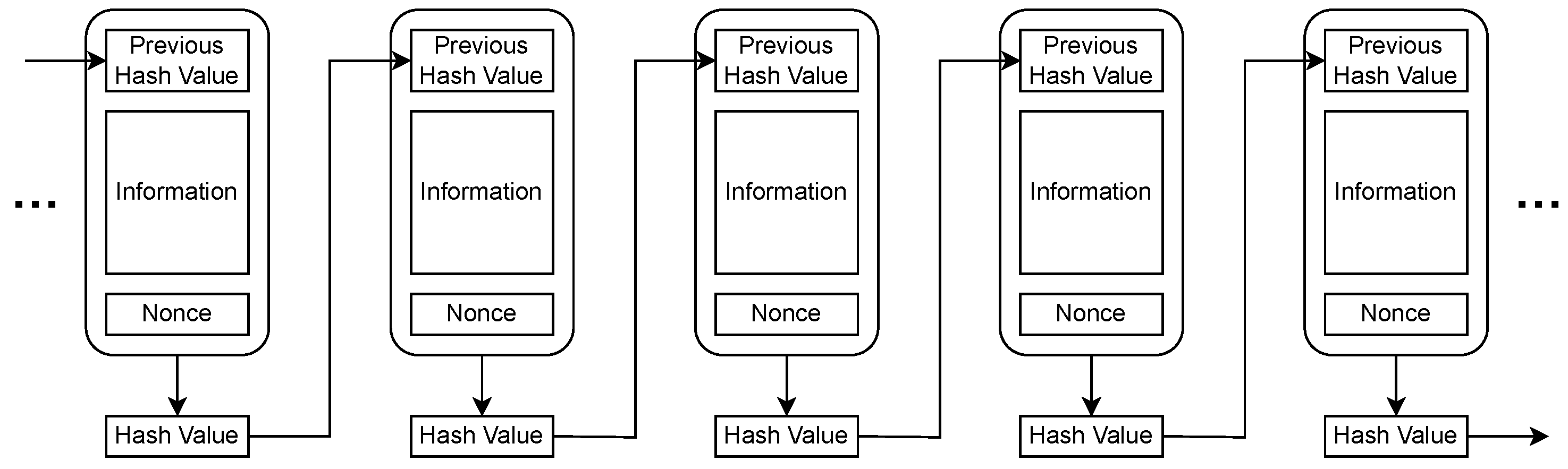
Figure 1. Here, we describe a Proof-of-Work algorithm. The blockchain works by incorporating the hash value of the past block. When adding the next block, the nonce value must be adjusted to ensure that the hash value of the entire block meets certain conditions.
Confirmations of transactions in blockchains are accomplished by connecting the block containing the new information to the previous blocks. However, the process of adjusting the nonce value and obtaining the desired hash value imposes a certain degree of difficulty and cost on miners. All miners participating in the blockchain network perform the search for the desired hash value. To tamper with a block at a given point in time, it is necessary to recalculate the hash values of all subsequent blocks, which implies paying the cost of a majority of miners participating in the blockchain network and is considered practically difficult [
15].
In major blockchain networks such as Bitcoin [
12], the confirmation process is conducted via a first-price auction. The decision of which transactions to include in a block is left to the miners, and it is the best choice for the miners to prioritize users who pay higher transaction fees [
16]. Therefore, high-fee users are prioritized, and low-fee users are put on hold. However, first-price auctions include the risk of overpaying and the difficulty of estimating fees [
17].
Ethereum adopted a new algorithm instead of first-price auctions to overcome this inefficiency. In the new algorithm, a transaction fee is comprised of base and priority fees.
The base fee is determined by the system, not the user. It is determined by how many transactions are included in the previous block. In other words, the base fee is controlled by the congestion level of the blockchain network. The formula for calculating the base fee is shown in (
1). Let the base fee of the t-th block be
, the maximum change rate per block be
d, the batch size of the t-th block be
, and the maximum batch size be
T. Here,
d is set to 0.125. The base fee increases by 12.5% over the previous base fee when the previous batch size is the maximum. It remains the same when it is half the maximum. It decreases by 12.5% when it is zero. Importantly, if the base fee is higher than the fee suggested by the user, the transaction will not be processed. Thus, users must suggest a higher fee or wait until the base fee decreases.
The priority fee is determined at the discretion of the user. Since the base fee is the same for all users, users are prioritized only based on the priority fee.
3. Related Work
Blockchain consensus algorithms have been evaluated and improved since blockchain was first proposed [
18,
19]. The consensus algorithm is still in need of improvement in terms of several evaluation metrics, such as processing speed, profitability, degree of decentralization, security, etc. [
20].
Along with the improvement of consensus algorithms, several studies have been conducted on approval times, with the main focus on using machine learning models for prediction [
21,
22]. However, these methods are considered vulnerable to extrapolation because they learn trends from historical data [
23]. They also require a large amount of data and high computational costs [
24,
25].
Several researchers have evaluated the performance of consensus algorithms using queueing theory [
10,
11]. Research has been conducted on models such as those that include the time taken to synchronize a blockchain network [
26] and those in which arrivals follow a Markovian arrival process and services follow a phase-type distribution [
27]. In addition, a model that takes into account the initial state of the queue has been proposed to improve the accuracy of the prediction of the length of stay [
28]. These studies are based on and extend the priority M/
/1 queueing model.
These studies were performed on models of first-price auctions and were not tested on the base fee algorithm. It is important to analyze the base fee algorithm because the second-largest major blockchain networks use it. In this paper, we model and analyze this algorithm.
4. Model
In this study, we analyze the base fee algorithm using a priority queueing model. This section describes the analytical model.
In the Ethereum architecture, the base fee is a continuous value, and the amount paid by users is also continuous. However, to simplify the analysis, we assume two levels of the base fee and the amount paid by users: high and low. We refer to users who pay high fees as high-priority customers and users who pay low fees as low-priority customers. The arrivals of high-priority and low-priority users are assumed to follow Poisson processes, where the arrival rate of low-priority customers is , and that of high-priority customers is .
We do not take priority fees into account. We assume that users form two queues based on the price they pay, and queues with the same price are admitted on a first-in, first-out basis.
In a blockchain, the time to generate a block is often significantly shorter than the time to calculate a nonce value. Thus, the service itself, block generation, was assumed to occur instantaneously in this model, and the time to calculate a nonce value is assumed to be the service time interval. We assume that the service time interval follows an exponential distribution with the mean
. In a blockchain system, a service is completed when a hash calculation is successful. The hash computations can be regarded as independent Bernoulli trials. Moreover, due to the high computational complexity of hashing, the time until the first successful computation in the entire system, i.e., the service time interval, follows an exponential distribution [
29].
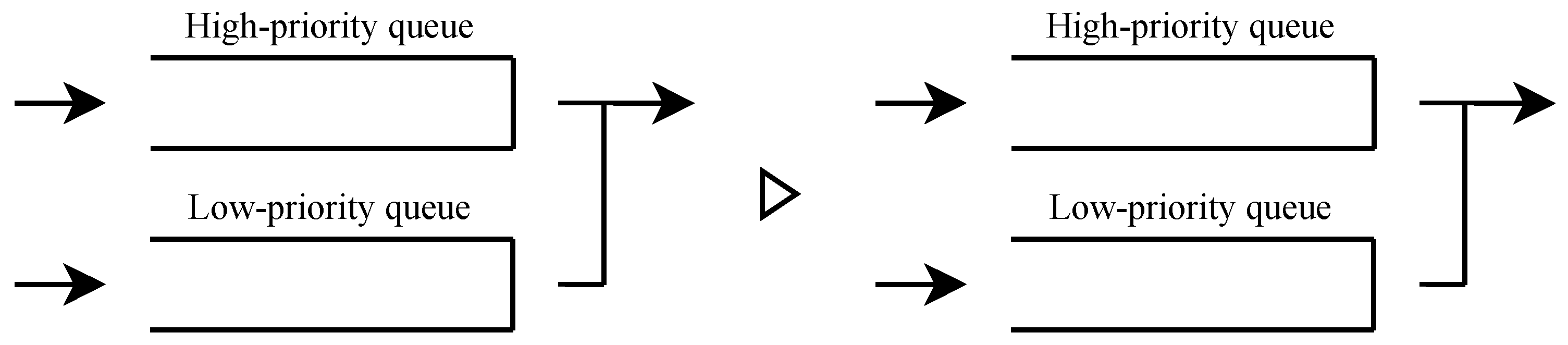
To replicate the base fee algorithm, we define two approval conditions: one in which all users can be approved and the other in which only users with high fees can be approved. The former corresponds to a case where the base fee is low, and the latter corresponds to a case where the base fee is high. We incorporate an algorithm changing the base fee depending on the conditions of the previous transaction into our model.
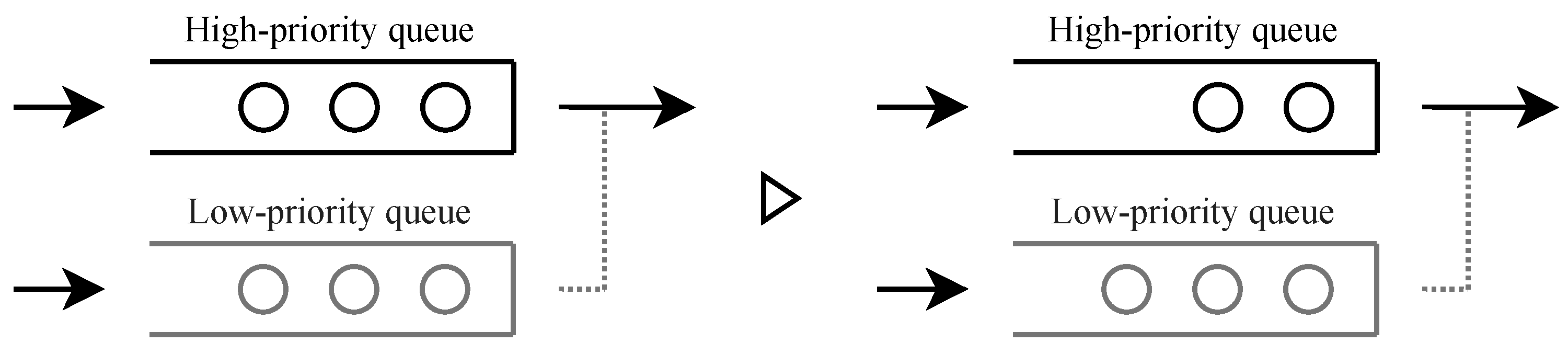
When there are available users, one user is admitted, and the next base price is higher. In contrast, when there is no available user, the system admits no user, and the next base price is lower. When both high- and low-priority users are waiting, the high-priority user is admitted. The decision as to who is served or not will be made at the end of the service interval. Four types of approval condition transitions are shown in
Figure 2,
Figure 3,
Figure 4 and
Figure 5.
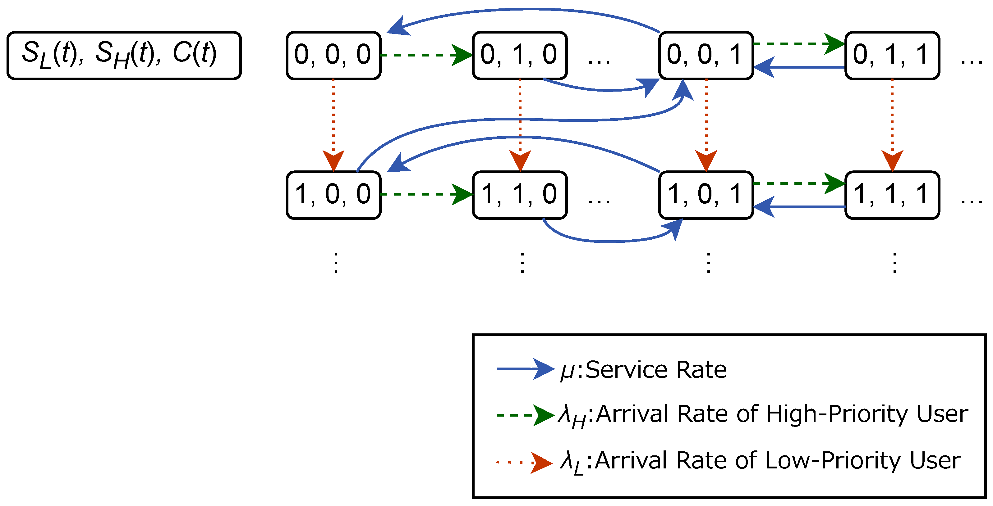
In the following, the queue length at time t is denoted by for the low-priority users and for the high-priority users. These include the next users to be served. The approval condition at time t is denoted by , where is the state in which all users can be approved, and is the state in which only the high-priority users can be approved.
We model the algorithm adopted in the blockchain network by incorporating changes in approval conditions based on the previous approval status into the model.
Figure 6 shows the state transition diagram of the model. The model differs from a typical priority queue with interruptions in that the service is provided immediately and must be provided multiple times to handle low-priority users. In addition, whereas other studies using queueing theory [
26,
27,
28] are based on first-price auctions, we model a system based on the base fee algorithm. Therefore, we incorporate the approval status into our model.
5. Performance Analysis
In this section, we calculate the performance evaluation index for the model in the previous section.
5.1. Stability Condition of High-Priority Queue
First, we consider the stability conditions of the high-priority queue. The high-priority queue is independent of the state of the low-priority queue since the high-priority users are approved first. The high-priority queue is also independent of the approval condition since the high-priority user can be approved regardless of the approval condition. Therefore, the high-priority queue depends on only two factors: the arrival rate of the high-priority users,
, and the service rate,
. Thus, the high-priority queue can be considered an M/M/1 queue. The stability condition for the high-priority queueing model is the same as that for the M/M/1 queueing model and is given by (
2). Note that
is the traffic density in the high-priority queue.
5.2. Stability Condition of Low-Priority Queue
Second, we consider the stability conditions for the low-priority queue. The low-priority users are approved only when the high-priority queue is zero and the server state is such that all users are served, as shown in
Figure 7. Therefore, the effective service rate of the low-priority queue can be expressed as
, where p is the probability that the high-priority queue is zero and the server state is that all users are served.
We consider the behavior of the partial model under the condition that the low-priority queue length is one or more. This assumption is valid in a situation where the arrival rate of the low-priority queue is non-zero, and we are concerned with the stability of low-priority customers (also known as the saturated rule, i.e., we only need to consider the stability of the number of low-priority customers when this number is large enough (at least 1)). The state transition diagram of the high-priority queue length,
, and the approval condition,
, is shown in
Figure 8. Accordingly, the partial model is a Markov chain because the current state determines the transition probabilities.
From
Figure 8, the transition rate matrix
of the high-priority queue length,
, and the approval condition,
, is given by (
3) at
.
where
is a zero matrix of appropriate dimensions.
We define the stationary distribution for this Markov chain as follows:
, where
, and where
Since the transition matrix, , is a block-tridiagonal matrix, the pair of the length of the high-priority queue, , and the approval condition, , is a QBD process.
From the theory of QBD, there exists (generally) a rate matrix,
, such that (
5).
The global equilibrium equation is given by (
6).
Furthermore, we obtain (
7) from the normalization condition of the probability distribution.
where
is a column vector of appropriate dimension in which all elements are 1.
In QBD, the rate matrix,
, satisfies the minimal non-negative solution of (
8).
Here, the rate matrix,
, is the 2-by-2 matrix given in (
9).
where
because
,
, and
are upper triangular matrices.
The component representation of (
8) is (
10). From this, the system of Equation (
11) can be derived.
The rate matrix,
, is the minimum non-negative solution of (
11), which is (
12).
From (
6) and (
7), we have (
13) and (
14).
where
is an identity matrix of appropriate dimensions.
By solving (
13) and (
14),
is obtained as (
15).
Since the rate matrix is an upper triangular matrix, the eigenvalues are and . Since and , the maximum eigenvalue is . The stability condition for this model is since the largest eigenvalue of must be less than 1. This exactly coincides with the stability condition for the high-priority queue.
It should be noted that
can be derived using the generating function approach. Indeed, we define generating functions as follows.
Balancing the equations of states
(
) yields
Furtheremore, from the balanced equations for states
and some transformation, we obtain
Because
, we also obtain (
15).
The service follows an exponential distribution. Therefore, according to Poisson arrivals (see time averages [
30]), the certain probability, p, where the high-priority queue is zero and the server state is that all users are served when the service is performed is equivalent to the steady state probability,
. The stability condition of the low-priority queue can be expressed as (
16) using the effective service rate. Note that
is the traffic density in the low-priority queue.
The above analysis indicates that significantly influences the stability condition of the low-priority queue.
5.3. Stability Condition of the Model
When both the high-priority and the low-priority queues are stable, the model is stable. Therefore, the stability condition for the entire model is given by (
17).
5.4. Stationary Probability
We derive the performance evaluation index of the model. Based on
Figure 6, the transition rate matrix,
, is (
18) by approximating the upper limit of the size of the high-priority queue to be
K. When the high-priority queue satisfies the stability condition, it is possible to obtain an approximate solution with arbitrary precision by setting a sufficiently large
K.
where
,
,
, and
are
matrices. Therefore, the stationary probability can be analyzed using QBD. We define the stationary probability
as (
19). In addition, let
, where
,
.
Similar to the model in
Figure 8, there exists a rate matrix,
, that satisfies (
20) when the low-priority queue length is greater than or equal to 1.
The global equilibrium equation is given by (
21).
Furthermore, we obtain (
22) from the normalization condition of the probability distribution.
In QBD, the rate matrix,
, satisfies (
23) due to (
20) and (
21).
Since
,
, and
are non-negative,
is a strictly diagonally dominant matrix. Therefore,
is an invertible matrix. Consequently, (
23) can be transformed into the form of (
24).
Based on (
24), we set
and repeat the calculations using (
25) to find
. At this time, it is known that the rate matrix,
, can be found by (
26). In numerical calculations, the calculation is stopped at n, where
is sufficiently small.
Furthermore, (
27) and (
28) hold from (
21) and (
22). Therefore, the stationary probability can be found by numerical calculation.
5.5. Average Number of Customers
The average number of customers in the high-priority queue,
, is derived from the M/M/1 queue and is given by (
29). The average number of customers in the low-priority queue
is derived from the QBD and is given by (
30).
5.6. Average Waiting Time
From Little’s law [
31], the average waiting time in the high-priority queue,
, and in the low-priority queue,
, are given by (
31) and (
32), respectively.
6. Numerical Simulation
We perform Monte Carlo simulations of the queueing model using Python 3.9 and compare the results with the theoretical values described above. In the following, one event is defined as an arrival or a service. The simulation is performed for 1,000,000 events for each parameter set, and the first 100,000 events are deleted to eliminate dependence on the initial state, resulting in 900,000 events.
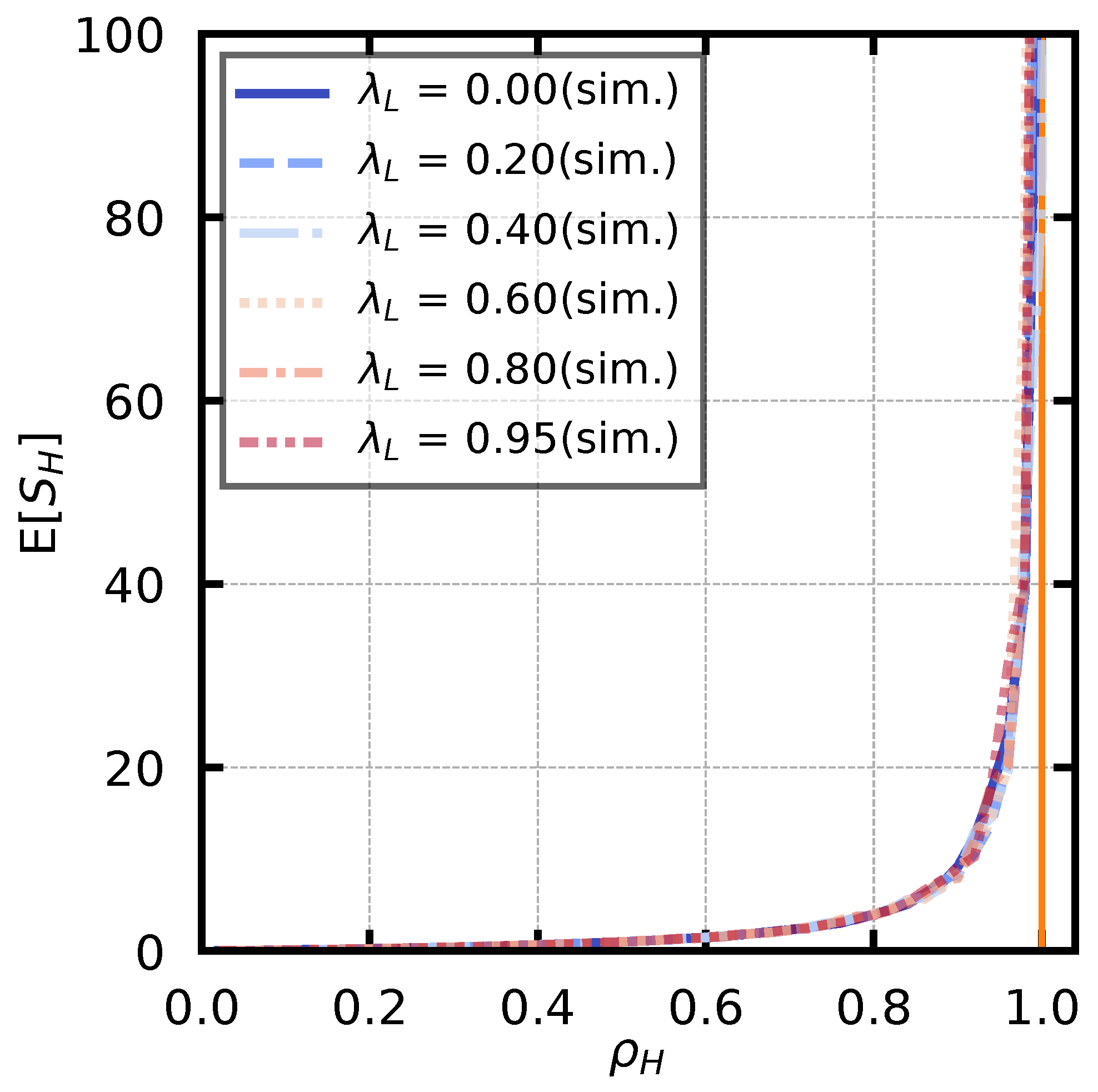
6.1. Stability Condition of the High-Priority Queue
The stability condition for the high-priority queue is given by (
2). The service rate is fixed at
, and the arrival rate of low-priority customers is set as
. We also derive the arrival rate of high-priority users,
, using (
2) so that
takes a value from
to
in steps of
. For each parameter set, we calculate the average number of customers of the high-priority queue,
, under the stability condition. The simulation results are shown in
Figure 9. Note that an auxiliary line is drawn at
, which is the boundary of the stability condition.
The figure shows that increases exponentially as approaches 1, independently of , and diverges when is greater than or equal to 1. All the lines overlap because they vary independently of .
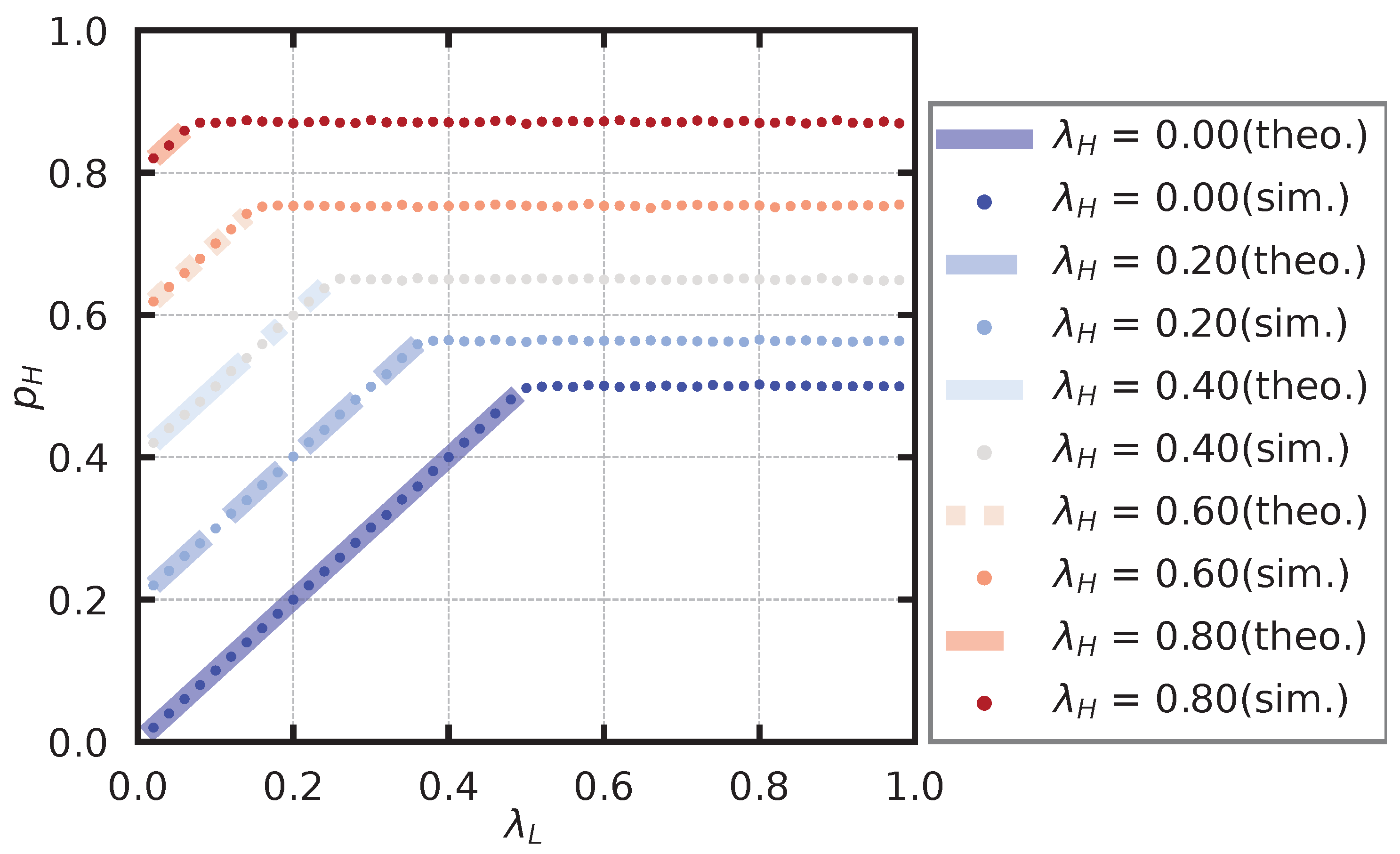
6.2. Stability Condition of the Low-Priority Queue
First, we verify
to derive stability conditions for low-priority queues. The theoretical value of
is given by (
15). In addition, simulations are performed under the same condition as in
Figure 8. The service rate is fixed at
. We derive the arrival rate of the high-priority users
based on (
2) such that
takes a value from
to
in steps of
. Theoretical and simulated values are shown in
Figure 10. From the figure, it can be seen that the theoretical values and simulation values generally agree.
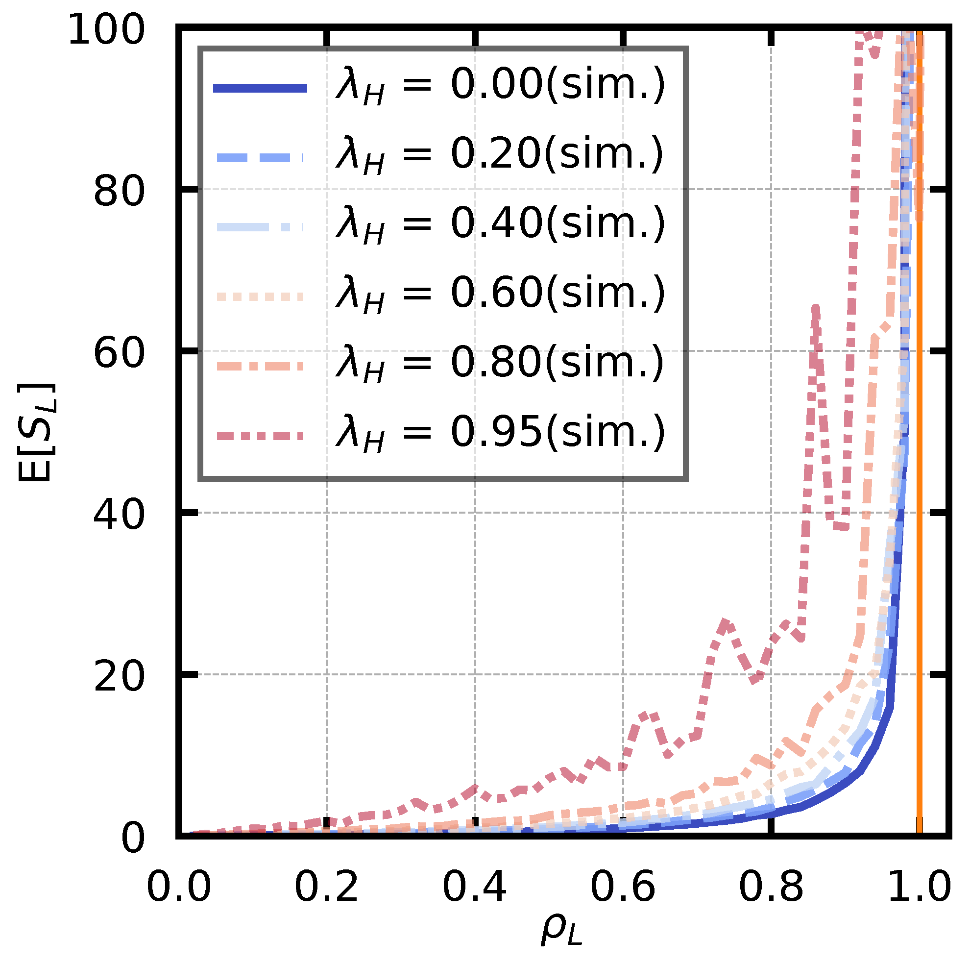
Second, we examine the stability conditions of the low-priority queue. The theoretical value is given by (
16). In addition, a simulation is performed under the same condition as in
Figure 6. The service rate is fixed at
, and the arrival rate of high-priority users is set as
. We derive the arrival rate of the low-priority user
based on (
16) such that
takes a value from
to
in steps of
. For each parameter set, we derive the average number of customers of the low-priority customer,
. The simulation results are shown in
Figure 11. Note that an auxiliary line is drawn at
, which is the boundary of the stability condition. The figure shows that
increases exponentially as
approaches 1, and
diverges when
is greater than or equal to 1.
6.3. Stationary Probability
We conduct a numerical experiment to find the stationary probability of the server state. The probability that only high-priority users can be approved is
, and its theoretical value is found by (
33).
We compare the theoretical value obtained by QBD with the simulated value.
In deriving the theoretical solution, the upper limit of the size of the high-priority queue, K, is set at 200. The repeated calculations of
are stopped at n when the maximum value of the elements of
is less than
. The service rate is fixed at
, and the arrival rate of high-priority users is set as
. In addition, the arrival rate of the low-priority users,
, is set from
to
in steps of
. For each parameter set, we calculate the probability that only high-priority users can be approved,
. The theoretical and simulated results are shown in
Figure 12. Note that locations where
does not satisfy the stability condition of the low-priority queue are not listed because there is no theoretical value.
From the figure, it seems that the theoretical and simulation values show similar trends in the region where the low-priority queue satisfies the stability.
When the low-priority queue satisfies the stability, changes linearly with . When the low-priority queue does not satisfy the stability, is constant, independent of . This is because when does not satisfy the stability condition, diverges, and there are always users waiting for the service.
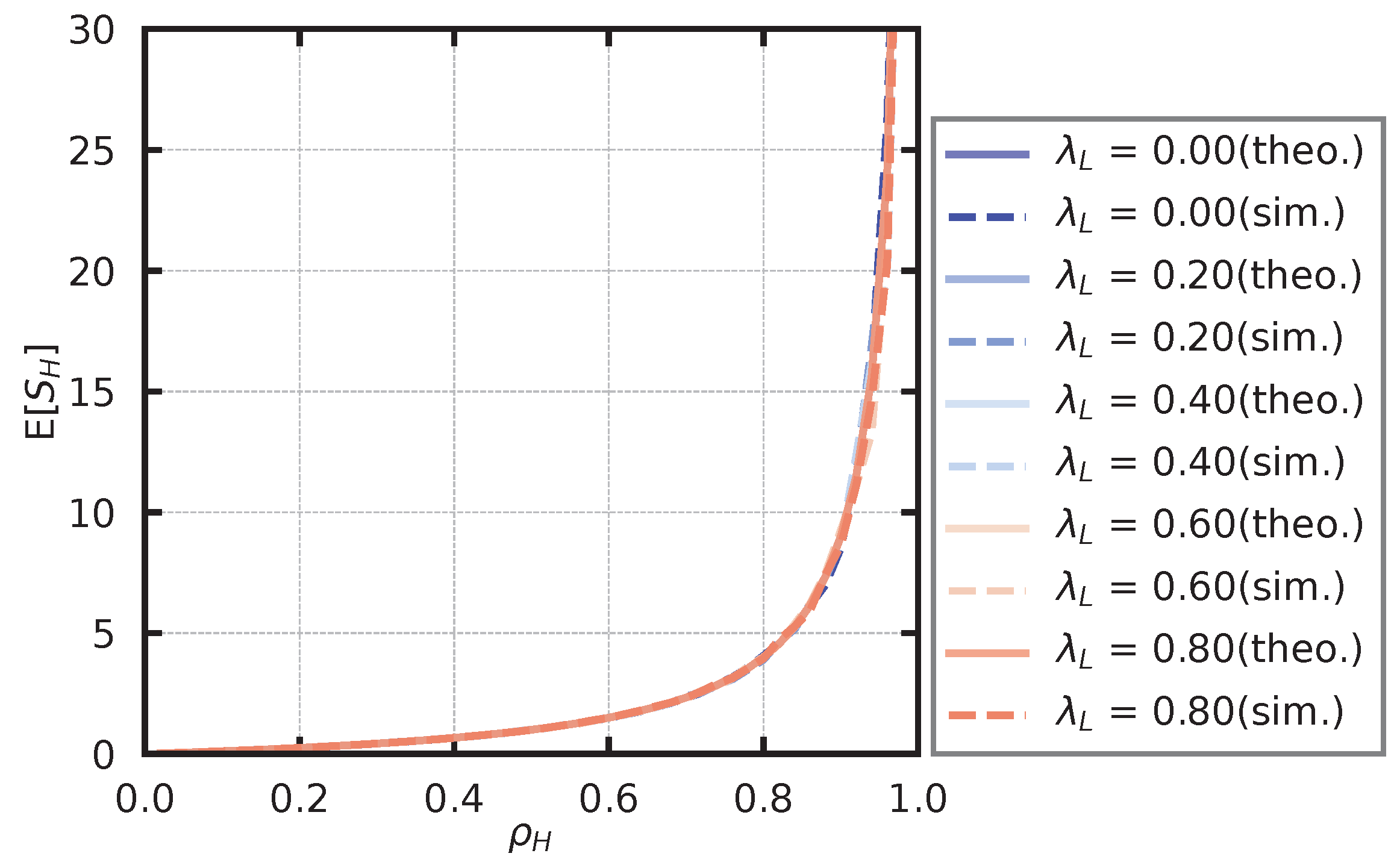
6.4. Average Number of Customers and Average Waiting Time
In deriving the theoretical solution, the upper limit of the size of the high-fee queue, K, is set at 200. The repeated calculations of are stopped at n when the maximum value of the elements of is less than .
In the simulation of the high-priority queue, the service rate is fixed at
, and the arrival rate of the low-priority user is set as
. We also derive the arrival rate of high-priority users
(
2) so that
takes a value from
to
in steps of
. For each parameter set, we derive the average number of customers in the high-priority queue,
, and the average waiting time in the high-priority queue,
. The theoretical and simulated values of the average number of customers are shown in
Figure 13, and the theoretical and simulated values of the average waiting time are shown in
Figure 14. From
Figure 13 and
Figure 14, we observe that
and
do not depend on
. Moreover, we observe that the theoretical values and simulation values generally agree.
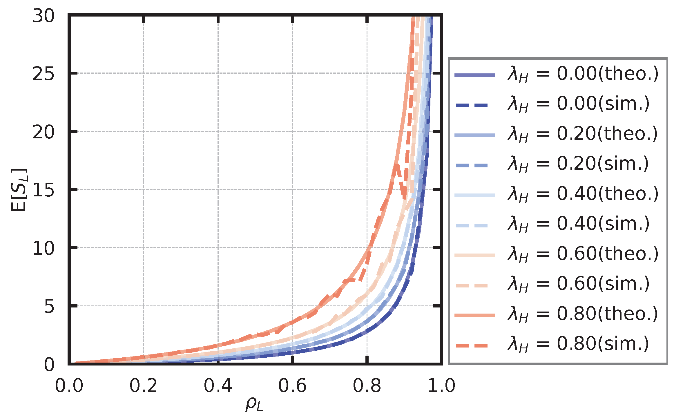
In the simulation of the low-priority queue, the service rate is fixed at
, and the arrival rate of the high-priority user is set as
. We derived the arrival rate of the low-priority user,
, based on (
16) such that
takes a value from
to
in steps of
. For each parameter set, we derived the average number of customers in the low-priority queue,
, and the average waiting time in the low-priority queue,
. The theoretical and simulated values of the average number of customers are shown in
Figure 15, and the theoretical and simulated values of the average waiting time are shown in
Figure 16. From
Figure 15 and
Figure 16, it seems that the theoretical and simulation values generally agree.
7. Conclusions
We modeled dynamic transaction fees considering approval conditions and derived stability conditions, stationary probability, average number of customers, and waiting time. Simulations validated our theoretical results. We proposed analyzing the low-priority queue’s stability using the result of the high-priority queue and approximating the stationary probability via QBD by limiting the number of customers in the high-priority queue. We also showed that the high-priority queue follows an M/M/1 model. In particular, the analytical solution of the stability condition makes it possible to determine the required service rate for the arrival rate, which contributes to determining the difficulty in blockchain.
This research facilitates the evaluation of existing systems and the design of more efficient alternatives. Further advancements in this study are expected to contribute to developing a cost-effective and high-speed blockchain. Moreover, our model appears to be applicable to systems with price fluctuations. However, several challenges remain. First, our model assumes a single-service system, whereas typical blockchains adopt batch processing, necessitating an extension to batch services. Second, this theory does not consider potential attacks or temporary blockchain branching, which should be incorporated for a more realistic analysis, as in previous studies [
32,
33]. Third, our current model treats transaction fees as discrete values, while in practice, fees often vary continuously; thus, extending the model to incorporate continuous fee structures is an important future direction. Finally, after extending the model to more realistic blockchain systems, we will evaluate how well the analyzed model aligns with real-world scenarios.
Author Contributions
Conceptualization, K.I. and T.P.-D.; Methodology, K.I. and T.P.-D.; Software, K.I.; Validation, K.I. and T.P.-D.; Formal analysis, K.I. and T.P.-D.; Investigation, K.I. and T.P.-D.; Writing—original draft, K.I.; Writing—review & editing, T.P.-D.; Visualization, K.I.; Supervision, T.P.-D. All authors have read and agreed to the published version of the manuscript.
Funding
The research of Tuan Phung-Duc was supported in part by JSPS KAKENHI, Grant Number 21K11765 and by F-MIRAI: R & D Center for Frontiers of MIRAI in Policy and Technology, the University of Tsukuba and Toyota Motor Corporation collaborative R & D center, Japan.
Data Availability Statement
No new data were created or analyzed in this study.
Conflicts of Interest
The authors declare no conflicts of interest.
References
- Zheng, Z.; Xie, S.; Dai, H.N.; Chen, X.; Wang, H. Blockchain challenges and opportunities: A survey. Int. J. Web Grid Serv. 2018, 14, 352–375. [Google Scholar]
- Zou, W.; Lo, D.; Kochhar, P.S.; Le, X.B.D.; Xia, X.; Feng, Y.; Chen, Z.; Xu, B. Smart contract development: Challenges and opportunities. IEEE Trans. Softw. Eng. 2019, 47, 2084–2106. [Google Scholar] [CrossRef]
- Kumar, S.; Dohare, U.; Kaiwartya, O. FLAME: Trusted Fire Brigade Service and Insurance Claim System Using Blockchain for Enterprises. IEEE Trans. Ind. Inform. 2023, 19, 7517–7527. [Google Scholar]
- Kumar, S.; Rathore, R.S.; Dohare, U.; Kaiwartya, O.; Lloret, J.; Kumar, N. BEET: Blockchain Enabled Energy Trading for E-Mobility Oriented Electric Vehicles. IEEE Trans. Mob. Comput. 2024, 23, 3018–3034. [Google Scholar]
- Easley, D.; O’Hara, M.; Basu, S. From mining to markets: The evolution of bitcoin transaction fees. J. Financ. Econ. 2019, 134, 91–109. [Google Scholar]
- Chaudhry, N.; Yousaf, M.M. Consensus Algorithms in Blockchain: Comparative Analysis, Challenges and Opportunities. In Proceedings of the 2018 12th International Conference on Open Source Systems and Technologies (ICOSST), Lahore, Pakistan, 19–21 December 2018; pp. 54–63. [Google Scholar]
- Nguyen, G.T.; Kim, K. A survey about consensus algorithms used in blockchain. J. Inf. Process. Syst. 2018, 14, 101–128. [Google Scholar]
- Wood, G. Ethereum: A secure decentralised generalised transaction ledger. Ethereum Proj. Yellow Pap. 2014, 151, 1–32. [Google Scholar]
- Reijsbergen, D.; Sridhar, S.; Monnot, B.; Leonardos, S.; Skoulakis, S.; Piliouras, G. Transaction Fees on a Honeymoon: Ethereum’s EIP-1559 One Month Later. In Proceedings of the 2021 IEEE International Conference on Blockchain (Blockchain), Melbourne, Australia, 6–8 December 2021; pp. 196–204. [Google Scholar]
- Kasahara, S.; Kawahara, J. Effect of Bitcoin fee on transaction-confirmation process. J. Ind. Manag. Optim. 2019, 15, 365–386. [Google Scholar]
- Kawase, Y.; Kasahara, S. Transaction-confirmation time for bitcoin: A queueing analytical approach to blockchain mechanism. In Proceedings of the Queueing Theory and Network Applications: 12th International Conference, QTNA 2017, Qinhuangdao, China, 21–23 August 2017; Springer: Berlin/Heidelberg, Germany, 2017. Proceedings 12. pp. 75–88. [Google Scholar]
- Nakamoto, S. Bitcoin: A Peer-to-Peer Electronic Cash System. 2008. Available online: https://assets.pubpub.org/d8wct41f/31611263538139.pdf (accessed on 10 January 2024).
- Buterin, V. A next-generation smart contract and decentralized application platform. White Pap. 2014, 3, 1–36. [Google Scholar]
- Vujičić, D.; Jagodić, D.; Ranđić, S. Blockchain technology, bitcoin, and Ethereum: A brief overview. In Proceedings of the 2018 17th International Symposium INFOTEH-Jahorina (INFOTEH), East Sarajevo, Bosnia and Herzegovina, 21–23 March 2018; pp. 1–6. [Google Scholar]
- Malakhov, I.; Marin, A.; Rossi, S.; Smuseva, D. On the use of proof-of-work in permissioned blockchains: Security and fairness. IEEE Access 2021, 10, 1305–1316. [Google Scholar]
- Huberman, G.; Leshno, J.; Moallemi, C.C. An economic analysis of the bitcoin payment system. Columbia Bus. Sch. Res. Pap. 2019, 17, 92. [Google Scholar]
- Leonardos, S.; Monnot, B.; Reijsbergen, D.; Skoulakis, E.; Piliouras, G. Dynamical analysis of the eip-1559 ethereum fee market. In Proceedings of the 3rd ACM Conference on Advances in Financial Technologies, Arlington, VA, USA, 26–28 September 2021; pp. 114–126. [Google Scholar]
- Liu, Y.; Lu, Y.; Nayak, K.; Zhang, F.; Zhang, L.; Zhao, Y. Empirical Analysis of EIP-1559: Transaction Fees, Waiting Times, and Consensus Security. In Proceedings of the 2022 ACM SIGSAC Conference on Computer and Communications Security. Association for Computing Machinery, CCS ’22, Los Angeles, CA, USA, 7–11 November 2022; pp. 2099–2113. [Google Scholar]
- Mingxiao, D.; Xiaofeng, M.; Zhe, Z.; Xiangwei, W.; Qijun, C. A review on consensus algorithm of blockchain. In Proceedings of the 2017 IEEE International Conference on Systems, Man, and Cybernetics (SMC), Banff, AL, Canada, 5–8 October 2017; pp. 2567–2572. [Google Scholar]
- Bamakan, S.M.H.; Motavali, A.; Bondarti, A.B. A survey of blockchain consensus algorithms performance evaluation criteria. Expert Syst. Appl. 2020, 154, 113385. [Google Scholar]
- Butler, C.; Crane, M. Blockchain Transaction Fee Forecasting: A Comparison of Machine Learning Methods. Mathematics 2023, 11, 2212. [Google Scholar] [CrossRef]
- Kurri, V.; Raja, V.; Prakasam, P. Cellular traffic prediction on blockchain-based mobile networks using LSTM model in 4G LTE network. Peer-Peer Netw. Appl. 2021, 14, 1088–1105. [Google Scholar]
- Marcus, G. Deep learning: A critical appraisal. arXiv 2018, arXiv:1801.00631. [Google Scholar]
- Mahajan, D.; Girshick, R.; Ramanathan, V.; He, K.; Paluri, M.; Li, Y.; Bharambe, A.; Van Der Maaten, L. Exploring the limits of weakly supervised pretraining. In Proceedings of the European Conference on Computer Vision (ECCV), Munich, Germany, 8–14 September 2018; pp. 181–196. [Google Scholar]
- Thompson, N.C.; Greenewald, K.; Lee, K.; Manso, G.F. The computational limits of deep learning. arXiv 2020, arXiv:2007.05558. [Google Scholar]
- Li, Q.L.; Ma, J.Y.; Chang, Y.X. Blockchain queue theory. In Proceedings of the Computational Data and Social Networks: 7th International Conference, CSoNet 2018, Shanghai, China, 18–20 December 2018; Springer: Berlin/Heidelberg, Germany, 2018. Proceedings 7. pp. 25–40. [Google Scholar]
- Li, Q.L.; Ma, J.Y.; Chang, Y.X.; Ma, F.Q.; Yu, H.B. Markov processes in blockchain systems. Comput. Soc. Netw. 2019, 6, 1–28. [Google Scholar]
- Malakhov, I.; Marin, A.; Rossi, S. Analysis of the confirmation time in proof-of-work blockchains. Future Gener. Comput. Syst. 2023, 147, 275–291. [Google Scholar]
- Kasahara, S. Performance Modeling of Bitcoin Blockchain: Mining Mechanism and Transaction-Confirmation Process. IEICE Trans. Commun. 2021, E104.B, 1455–1464. [Google Scholar]
- Wolff, R.W. Poisson arrivals see time averages. Oper. Res. 1982, 30, 223–231. [Google Scholar] [CrossRef]
- Little, J.D. A proof for the queuing formula: L=λW. Oper. Res. 1961, 9, 383–387. [Google Scholar] [CrossRef]
- Kim, S.K. Blockchain Governance Game. Comput. Ind. Eng. 2019, 136, 373–380. [Google Scholar] [CrossRef]
- Kim, S.K. Strategic Alliance for Blockchain Governance Game. Probab. Eng. Informational Sci. 2020, 36, 1–17. [Google Scholar] [CrossRef]
Figure 1.
Blockchain diagram. A block is composed of the previous hash value, information, and nonce. The information part can have any content. The nonce is a value adjusted so that the hash value of the entire block meets a certain condition.
Figure 1.
Blockchain diagram. A block is composed of the previous hash value, information, and nonce. The information part can have any content. The nonce is a value adjusted so that the hash value of the entire block meets a certain condition.
Figure 2.
When service occurs in a state where only high-priority users are served, one high-priority user is served, and the state where only high-priority users are served continues.
Figure 2.
When service occurs in a state where only high-priority users are served, one high-priority user is served, and the state where only high-priority users are served continues.
Figure 3.
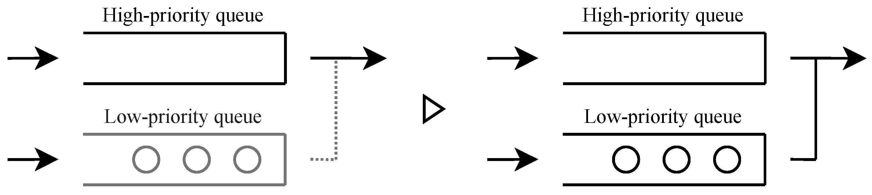
When service occurs in a state where only high-priority users are served, no user can receive the service. Thus, the system transitions to a state where all users can receive service.
Figure 3.
When service occurs in a state where only high-priority users are served, no user can receive the service. Thus, the system transitions to a state where all users can receive service.
Figure 4.
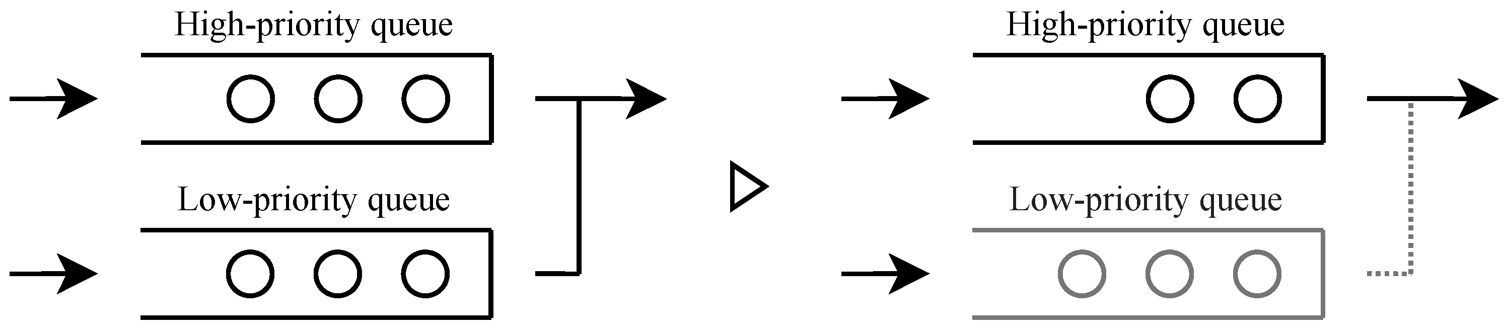
When service occurs in the state where all users are served, a high-priority user is served preferentially. When there is no high-priority user, a low-priority user is served. Thus, the system transitions to a state where only high-priority users are served.
Figure 4.
When service occurs in the state where all users are served, a high-priority user is served preferentially. When there is no high-priority user, a low-priority user is served. Thus, the system transitions to a state where only high-priority users are served.
Figure 5.
When service occurs in a state where all users are served, and there is no user, then no user is served. Thus, the state where all users are served continues.
Figure 5.
When service occurs in a state where all users are served, and there is no user, then no user is served. Thus, the state where all users are served continues.
Figure 6.
Transition diagram of the entire model.
Figure 6.
Transition diagram of the entire model.
Figure 7.
When service occurs in a state where all users are served and there is no high-priority user, a low-priority user is served; thus, the system transitions to a state where only high-priority users are served.
Figure 7.
When service occurs in a state where all users are served and there is no high-priority user, a low-priority user is served; thus, the system transitions to a state where only high-priority users are served.
Figure 8.
Transition diagram of the high-priority queue length and the approval condition under the condition that the low-priority queue length is one or more.
Figure 8.
Transition diagram of the high-priority queue length and the approval condition under the condition that the low-priority queue length is one or more.
Figure 9.
Stability condition of high-priority queue. The vertical orange line is an auxiliary line indicating .
Figure 9.
Stability condition of high-priority queue. The vertical orange line is an auxiliary line indicating .
Figure 10.
against .
Figure 10.
against .
Figure 11.
Stability condition of low-priority queue. The vertical orange line is an auxiliary line indicating .
Figure 11.
Stability condition of low-priority queue. The vertical orange line is an auxiliary line indicating .
Figure 12.
Server status. The theoretical values are shown only under conditions that satisfy the stability conditions.
Figure 12.
Server status. The theoretical values are shown only under conditions that satisfy the stability conditions.
Figure 13.
Average number of high-priority users.
Figure 13.
Average number of high-priority users.
Figure 14.
Average waiting time of high-priority users.
Figure 14.
Average waiting time of high-priority users.
Figure 15.
Average number of low-priority users.
Figure 15.
Average number of low-priority users.
Figure 16.
Average waiting time of low-priority users.
Figure 16.
Average waiting time of low-priority users.
| Disclaimer/Publisher’s Note: The statements, opinions and data contained in all publications are solely those of the individual author(s) and contributor(s) and not of MDPI and/or the editor(s). MDPI and/or the editor(s) disclaim responsibility for any injury to people or property resulting from any ideas, methods, instructions or products referred to in the content. |
© 2025 by the authors. Licensee MDPI, Basel, Switzerland. This article is an open access article distributed under the terms and conditions of the Creative Commons Attribution (CC BY) license (https://creativecommons.org/licenses/by/4.0/).


