Accurate Approximation for Resource Queuing Systems with Losses and Signals

Abstract

We consider a queuing system with a finite number of servers and a finite pool of resources, where an arriving customer requires a server and random number of resources. During the service, each customer is associated with a Poisson flow of “signals”, where upon a signal arrival, the currently allocated resources for a customer are released, and an attempt is made to allocate a new random amount of resources. Recently, such systems have received significant attention for their use in the analysis of 5G/6G cellular systems with non-elastic traffic demands and blockage impairments. Such queuing systems do not allow closed-form analytical solutions, and are conventionally solved using numerical methods. These methods are sensitive to the dimensions of the state space and can lead to inaccuracies. In this paper, we propose a new method for the approximate analysis of performance metrics in resource systems with signals using analytical solutions for similar systems without signals. Our detailed comparison with simulations shows that the relative error is limited to 5–10% over a wide range of system and load parameters.

1. Introduction

Resource loss systems (ReLSs) are queuing systems, in which arriving customers require a server and a random amount of resources for service, which is determined based on a given probability distribution. ReLS generalizes the ideas of F.P. Kelly [1,2] for multiservice queues, where the customers of each arrival flow require a certain number of resource units. Initially, such models were utilized to analyze computing systems, where processor time, memory, and other resources can be limited [3,4]. Similar systems with non-elementary arrival and service processes and unlimited resources have also received attention [5,6]. Of course, resource loss systems are not the only class of queuing systems that use the principle of the heterogeneity of customer requirements. In the performance analysis of high-performance computing clusters, multiserver models are also considered, in which customers occupy a random number of servers upon arrival [7,8]. Unlike the ReLS, customer requirements can only take integer values. In addition, the theory of queuing-inventory systems has been actively developed over the past few decades [9,10]. In these models, customers do not return occupied resources at the end of the service process, and the inventory level is maintained by an additional replenishment process.

Recently, resource loss systems have found widespread application in the analysis of 5G and 6G cellular systems, where a limited number of signal processors and time–frequency resources are shared between arriving sessions [11]. In modern cellular systems utilizing millimeter wave (mmWave) and terahertz (THz) frequency bands, the time–frequency resource requirements of data transmission sessions can change drastically because of multiple factors, including random user locations and radio channel quality fluctuations, making the amount of resources required a random variable. To increase the coverage area, large antenna arrays are utilized that focus energy in a certain direction via a beamforming procedure. However, this means that when a small moving object such as a car or person crosses the propagation path, the received power drops sharply. As a result, to maintain the same bitrate during a session, a significant increase in frequency resources is required as demonstrated in [12,13]. In addition, user sessions can be interrupted because of the blockage of the propagation path between the user and a base station (BS) [12,14]. To account for this feature, conventional ReLS has been extended to include the so-called “signals” in [15]. Here, signals trigger resource reallocation for user sessions, that is, the session releases the currently occupied resources, generates new resource requirements, and attempts to continue its service. This type of model is frequently utilized for the analysis of 5G/6G mmWave/THz cellular network performance; see [13] for an overview.

The term “signals” was first introduced by Gelenbe [16,17] to describe the flow of external events that trigger changes in the customers’ service process in G-networks. These changes include changing the service node or resetting a batch of customers. In the system considered in this study, signals cause a change in resource requirements. Additionally, the intensity of the signal flow depends on the number of customers in the system.

Despite their important applications, no analytical solutions have yet been reported for ReLSs with signals. As a result, one must reply to the numerical solution of a system of equilibrium equations to derive stationary probabilities. However, this may lead to significant computational complexity because the state space of the system is usually large in practical applications. The authors of [15] proposed a method to approximate the main performance measures, including customer loss probability and system resource utilization. However, they noticed that the proposed approach was accurate for a limited range of system load conditions.

The aim of this study is to propose an accurate approximation method for the analysis of a ReLS queuing system with signals that are accurate for a wide range of system parameters and load conditions. This method is based on the solution of the ReLS with the same parameters but without signals for which an analytical solution exists [18]. A similar concept was applied to an approximate analysis of retrial queues [19]. The approximation is based on the assumption that retrials form an additional independent arrival (in most cases, Poisson) flow, whose intensity is implicitly determined by the conservation law [20,21]. Specifically, the authors in [20] showed that approximation accuracy decreases with a decrease in the time to retrial. In the ReLS with signals, customers try to re-enter the system immediately after signal arrival; therefore, one needs to improve the basic idea to provide a more reliable approximation. Our approach to approximating the loss probability of customers that re-enter the system upon signal arrival is based on the utilization of the stationary distribution at the departure epochs of the ReLS without signals. To assess the accuracy of the proposed approximation, we compared it with the results obtained from the numerical solution of a system of equilibrium equations for a wide range of load conditions.

The main contributions of our study are as follows:

• An accurate analytical approximation for the analysis of performance metrics in resource queuing systems with losses and signals, which is currently widely utilized for the performance analysis of 5G/6G cellular systems.
• A comparison with the exact solution obtained from the system of equilibrium equations demonstrates that the relative error is upper bounded by 5%–10% over a wide range of system and load parameters.

The remainder of this paper is organized as follows. In Section 2, we formalize the ReLS with signals. The proposed approximation is introduced in Section 3, including the derivation of the stationary distribution at departure epochs of the ReLS without signals. An accuracy analysis of the proposed method is presented in Section 4. Finally, Section 5 concludes the paper.

2. Resource Loss System with Signals

In this section, we begin by describing the model. We then introduce a stochastic process to describe the behavior of the system. Furthermore, we specify the associated balance equations. Finally, we demonstrate how to derive the metrics of interest, including customer loss probability, mean number of customers in the system, and system resource utilization.

2.1. Model Description

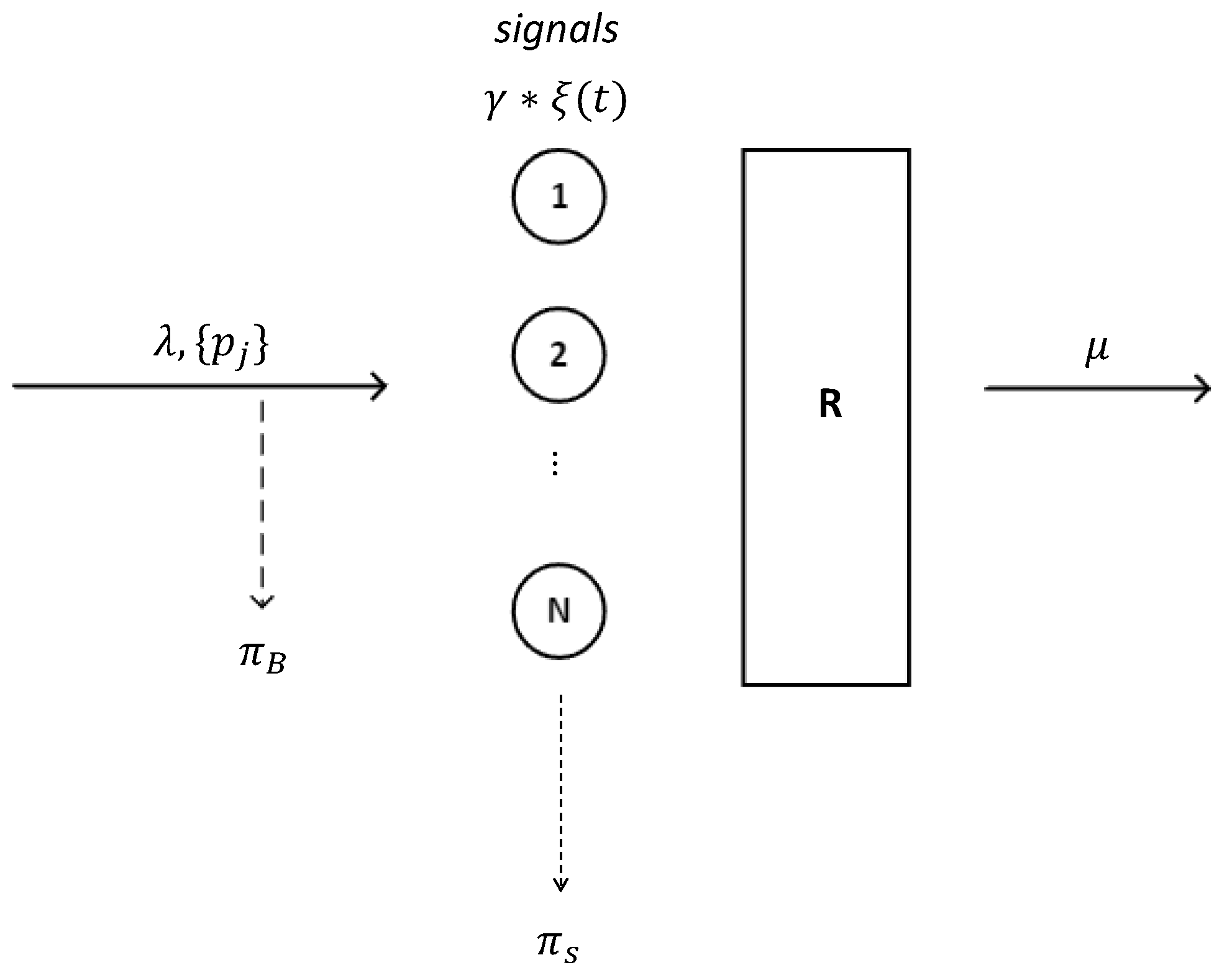
Consider a ReLS with N servers. The system is associated with a set of resources with R units. Customers arrive according to a Poisson process with intensity $\lambda$. Each customer requires a server and random number of resource units. The distribution of the number of requested resource units is determined by the probability mass function (pmf) $\left\{p_j\right\},0\le j\le R$. The resource requirements are assumed to be independent of the arrival and service processes. An arriving customer that requires r resource units is accepted for service if there is a free server and the total number of occupied resource units in the system does not exceed $R-r$. Otherwise, the customer is lost. The service times are exponentially distributed with an intensity $\mu$. At the end of service time, the customer releases the occupied resource volume.

Each customer in the system generates a Poisson flow of special events (signals) with an intensity $\gamma$. Upon the arrival of a signal from the corresponding flow, the customer releases the occupied resource volume, generates new resource requirements according to the same pmf $\left\{p_j\right\},0\le j\le R$ and tries to continue its service. If the number of unoccupied resource units is less than the new resource requirements of the customer, the service process is terminated and the customer leaves the system. Otherwise, the customer service process will continue. According to the memoryless property of exponential distribution, the residual service time of a customer upon signal arrival is exponentially distributed with the same intensity $\mu$. The proposed system is schematically shown in Figure 1.

Note that the pmf of the resource requirements can be described in a more general form without limitations on the maximum resource requirements, that is, $\left\{p_j\right\},j\ge 0$. However, customers whose requirements exceed the resource volume associated with the system do not change the system behavior, simply increasing the loss probability (upon arrival) by the tail of the distribution ${\sum }_{j=R+1}^{\infty }{p}_j$. Therefore, in the following, we assume ${\sum }_{j=0}^R{p}_j=1$ without loss of generality.

2.2. System’s Behavior

Let $X\left(t\right)=\{\xi \left(t\right),r_1\left(t\right),\cdots ,r_{\xi \left(t\right)}\left(t\right)\}$ be the Markov process that describes the behavior of the system. Here, $\xi \left(t\right)$ is the number of customers in the system at time t, and $r_i\left(t\right)$ is the number of resource units occupied by the i-th customer. The state space of $X\left(t\right)$ grows exponentially with the growth of R; the following simplified approach is often used for the analysis of ReLSs [18]. Instead of keeping track of the resource volumes occupied by each customer $(r_1\left(t\right),\cdots ,r_{\xi \left(t\right)}\left(t\right))$, we keep track of the sum of resource units occupied by all current customers together, $\delta \left(t\right)=r_1\left(t\right)+\cdots +r_{\xi \left(t\right)}\left(t\right)$. Therefore, we consider a stochastic process $Y\left(t\right)=\left\{\xi \right(t),\delta (t\left)\right\}$, where $\delta \left(t\right)$ is the total number of resource units occupied by all the customers.

Process $Y\left(t\right)$ is not Markovian, as the number of resource units to be released upon the departure of a customer depends on the resource requirements chosen upon its arrival to the system or the arrival of a signal. To handle this, we employ the Bayesian approach, and assume that a customer releases j resource units with probability

$${\displaystyle \frac{p_j{p}_{r-j}^{(n-1)}}{p_r^{\left(n\right)}}},$$

(1)

given that, just before departure, the system is in state $\left(\xi \right(t)=n,\delta (t)=r)$. Here, $p_r^{\left(n\right)}$ is the probability that n customers occupy exactly r resource units. Probabilities $\left\{p_r^{\left(n\right)}\right\}$ can be evaluated as n-fold convolution of the initial resource requirement distribution by the following recurrent relation:

$$p_r^{\left(n\right)}=\sum _{j=0}^r{p}_j{p}_{r-j}^{(n-1)},0\le r\le R, 1\le n\le N,$$

(2)

with initial values

$$p_0^{\left(0\right)}=1,p_r^{\left(0\right)}=0, r>0.$$

(3)

With the proposed approach, process $Y\left(t\right)$ for the simplified system becomes Markovian, but the volume of released resources upon customer departure may not coincide with the volume of occupied resources upon its arrival. It was shown in [18] that for a ReLS without signals, the stationary distribution of the number of customers and the total volume of occupied resources of the initial system with vector representation of occupied resources is equivalent to the corresponding distribution of the simplified system. Although there is no such equivalence in the considered system with signals, the proposed approach still results in a good approximation of stationary behavior [13].

2.3. System’s Balance Equations

The set of states of $Y\left(t\right)$ can be divided into $N+1$ disjoint subsets as

$$\begin{array}{c}\hfill S=\bigcup _{n=0}^N{S}_n,\hfill \\ \hfill S_n=\{(n,r):0\le r\le R,p_r^{\left(n\right)}>0\}.\hfill \end{array}$$

(4)

We now introduce the stationary probabilities:

$$\begin{array}{cc}\hfill & q_0=\underset{t\to \infty }{lim}P\left\{\xi \right(t)=0\},\hfill \\ \hfill & q_k\left(r\right)=\underset{t\to \infty }{lim}P\left\{\xi \right(t)=k,\delta (t)=r\},(k,r)\in X_k.\hfill \end{array}$$

(5)

To derive the balance equations that characterize the equilibrium behavior of the system, we must determine all possible events in the system and the corresponding state transitions. There are three types of events: (i) arrival of a customer, (ii) departure of a customer, and (iii) arrival of a signal. Assume that the system is in state $(n,r)$. An arriving customer that requires j resource units is accepted for service if $n<N$ and $r+j\le R$, and the system state is changed to $(n+1,r+j)$. Otherwise, the arriving customer is lost and the state remains unchanged. Upon the departure of a customer, the system state changes to $(n-1,r-j)$ with probability ${\displaystyle \frac{p_j{p}_{r-j}^{(n-1)}}{p_r^{\left(n\right)}}}$. Upon the arrival of a signal, the customer releases j resource units with the same probability and attempts to occupy i resource units with probability $p_i$. If $r-j+i\le R$, then its service continues, and the system moves to state $(n,r-j+i)$. Otherwise, the service process is terminated and the system state is changed to $(n-1,r-j)$.

Based on the events and transitions considered, the balance equations of $Y\left(t\right)$ can be written as follows:

$$\lambda q_0=\mu \sum _{j:(1,j)\in X_1}{q}_1\left(j\right),$$

(6)

for the empty state,

$$\begin{array}{cc}\hfill & \left(\lambda \sum _{j=0}^{R-r}{p}_j+k\mu +k\gamma \right)q_k\left(r\right)=\lambda \sum _{j\ge 0,(k-1,r-j)\in X_{k-1}}{q}_{k-1}(r-j)p_j+\hfill \\ \hfill & +(k+1)\mu \sum _{j\ge 0,(k+1,r+j)\in X_{k+1}}{q}_{k+1}(r+j){\displaystyle \frac{p_j{p}_r^{\left(k\right)}}{p_{j+r}^{(k+1)}}}+k\gamma \sum _{j:(k,j)\in X_k}{q}_k\left(j\right)\sum _{i=max(0,j-r)}^j{p}_{r-j+i}{\displaystyle \frac{p_i{p}_{j-i}^{(k-1)}}{p_j^{\left(k\right)}}}+\hfill \\ \hfill & +(k+1)\gamma \sum _{j\ge 0,(k+1,r+j)\in X_{k+1}}{q}_{k+1}(r+j){\displaystyle \frac{p_j{p}_r^{\left(k\right)}}{p_{j+r}^{(k+1)}}}\sum _{s=R-r+1}^R{p}_s, 1\le k\le N-1, (k,r)\in X_k,\hfill \end{array}$$

(7)

for the states with $1\le k\le N-1$,

$$\begin{array}{cc}\hfill & \left(N\mu +N\gamma \right)q_N\left(r\right)=\lambda \sum _{j\ge 0,(N-1,r-j)\in X_{N-1}}{q}_{N-1}(r-j)p_j+\hfill \\ \hfill & +N\gamma \sum _{j:(N,j)\in X_N}{q}_N\left(j\right)\sum _{i=max(0,j-r)}^j{\displaystyle \frac{p_i{p}_{j-i}^{(N-1)}}{p_j^{\left(N\right)}}}{p}_{r-j+i},(N,r)\in X_N.\hfill \end{array}$$

(8)

for the states with $k=N$.

Because the state space is limited and there is one set of ergodic states, the system of equilibrium in Equations (6)–(8), along with the normalization condition, has a unique solution that can be obtained numerically.

2.4. Performance Metrics

Equipped with the stationary probabilities of the system, the main metrics of interest can be derived. First, the probability that a customer is lost upon arrival ${\pi }_B$ is given by

$${\pi }_B=1-\sum _{(n,r)\in S,n<N}{q}_n\left(r\right)\sum _{j=0}^{R-r}{p}_j.$$

(9)

Then, we can evaluate the probability ${\pi }_s$ that the arrival of a signal causes the loss of a customer as

$${\pi }_s=\sum _{(n,r)\in S,n>0}{q}_n\left(r\right)\sum _{j=0}^r{\displaystyle \frac{p_j{p}_{r-j}^{(n-1)}}{p_r^{\left(n\right)}}}\left(1-\sum _{i=0}^{R-r+j}{p}_i\right).$$

(10)

Customers may experience multiple signal arrivals during their service times. The probability that the service process of an accepted customer is terminated (so-called termination probability) can be deduced as follows: In a long period T, the mean number of accepted customers is $\lambda (1-{\pi }_B)T$. At time T, the mean number of terminated customers is $\gamma \overline{N}{\pi }_{s}T$, where $\overline{N}$ denotes the mean number of customers in the system. Then, the termination probability ${\pi }_T$ is given by

$${\pi }_T=\underset{T\to \infty }{lim}{\displaystyle \frac{\gamma \overline{N}{\pi }_{s}T}{\lambda (1-{\pi }_B)T}}={\displaystyle \frac{\gamma \overline{N}{\pi }_s}{\lambda (1-{\pi }_B)}}$$

(11)

where $\overline{N}$ is given by

$$\overline{N}=\sum _{(n,r)\in S}n{q}_n\left(r\right).$$

(12)

Finally, we can evaluate the mean number of occupied resource units:

$$\overline{R}=\sum _{(n,r)\in S}r{q}_n\left(r\right).$$

(13)

3. Approximation of Stationary Characteristics

In this section, we introduce an approximate analysis of the ReLS with signals. We begin by describing the main idea, then proceed with derivations and finally introduce an iterative algorithm for the calculation of performance metrics.

3.1. The Main Idea

In the special case of the described ReLS without signals (i.e., $\gamma =0$), it is possible to obtain an analytical solution for the system of balance in Equations (6)–(8). It was shown in [18] that the stationary distribution in the discrete resource case is given by

$$\begin{array}{cc}\hfill & q_n\left(r\right)=q_0{\displaystyle \frac{{\rho }^n}{n!}}{p}_r^{\left(n\right)},1\le n\le N, 0\le r\le R,\hfill \end{array}$$

(14)

$$\begin{array}{cc}\hfill & q_0={\left(1+\sum _{n=1}^N\sum _{r=0}^R{\displaystyle \frac{{\rho }^n}{n!}}{p}_r^{\left(n\right)}\right)}^{-1}.\hfill \end{array}$$

(15)

An efficient algorithm for calculating the performance metrics of interest for $\gamma =0$ was developed in [22]. In what follows, we reply to this algorithm to extend it to the case of $\gamma \ne 0$.

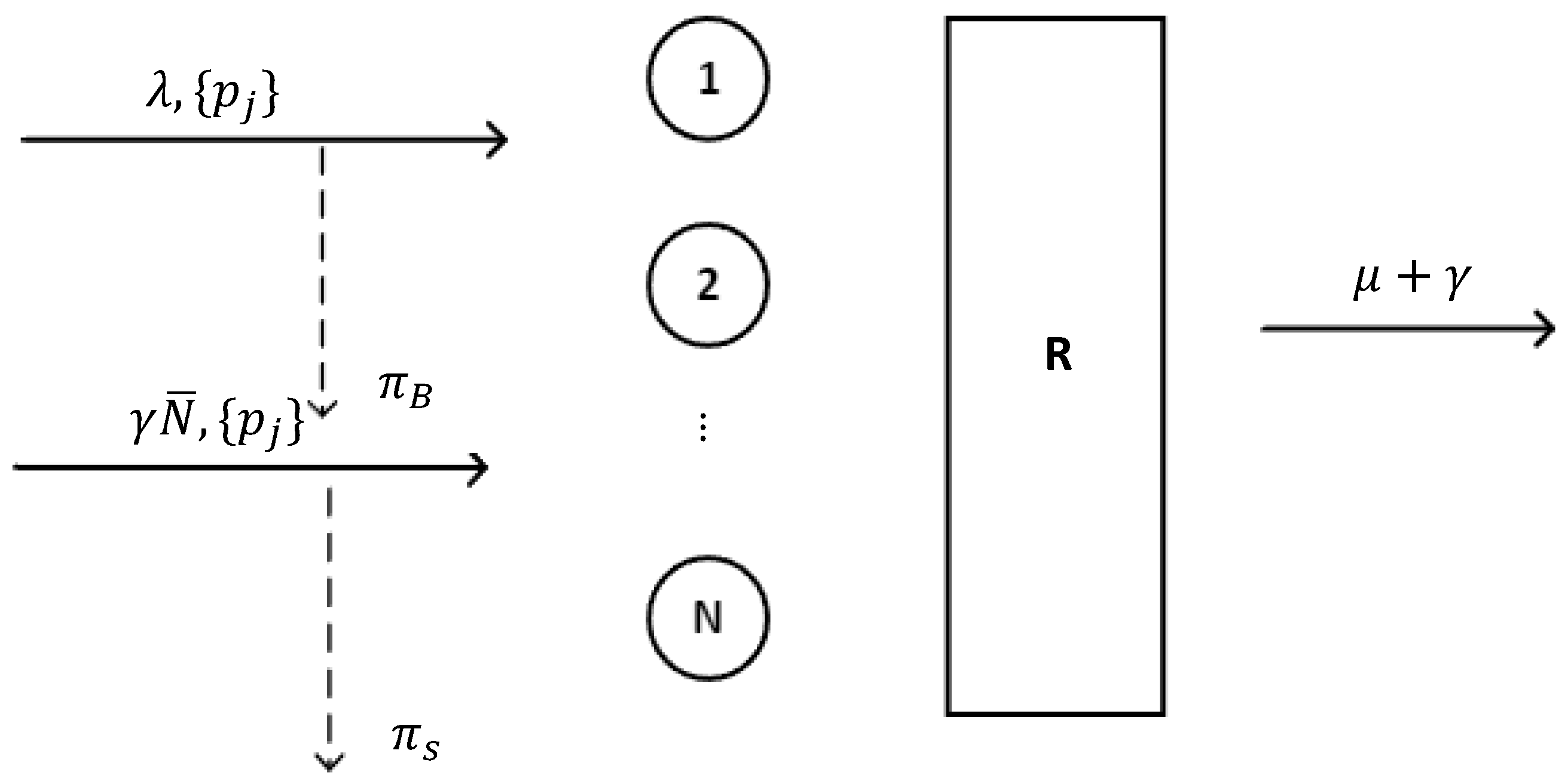
Consider the concept presented in [15]. The authors approximated the behavior of an ReLS with signals by the ReLS without signals but with an additional arrival flow, as discussed below. Assume that, upon arrival of a signal, the associated customer leaves the system, so the service intensity of customers is actually $\mu +\gamma$. However, with probability ${\displaystyle \frac{\gamma }{\mu +\gamma }}$, the customer returns to new resource requirements. We treated these returning customers as an additional arrival flow with an intensity $\overline{N}\gamma$, where $\overline{N}$ is the mean number of customers in the system. A schematic of the system is shown in Figure 2.

The approximation system has two arrival flows. We refer to these as primary and secondary customers, where secondary customers are those returning to the system upon signal arrival. In [15], it was assumed that the secondary customers formed another Poisson process. Because both types of customers have the same resource requirements (pmf), they can be aggregated into a single Poisson process with intensity $\lambda +\overline{N}\gamma$, and the analytical results for resource queuing systems without signals can be applied to evaluate performance metrics. Here, the termination probability in (11) can be interpreted as the loss probability of secondary customers.

The intensity of secondary customers can be estimated using the following iterative algorithm [15]. Specifically, we begin with the zero intensity of a secondary flow, evaluate the mean number $\overline{N}$ of customers in the system, and adjust the intensity of the secondary flow accordingly. This procedure continues until the desired accuracy is achieved.

The numerical results showed that the approach proposed in a previous paper provides an acceptable accuracy with a relative error of approximately 10% for the loss probability ${\pi }_B$ and the average number of occupied resource units $\overline{R}$, but not for the termination probability ${\pi }_T$. The termination probability can be evaluated by the described method with acceptable accuracy in more complex systems, where there are additional flows of customers that do not suffer from signal arrivals.

The main problem with this approach is that secondary customers do not arrive at arbitrary time instants. Upon arrival of a signal in the initial ReLS, the customer immediately re-enters the system with new resource requirements. This means that secondary customers arrive not at arbitrary epochs, but at the service completion epochs. Consequently, if the new resource requirements are less than or equal to the previous amount of resources, the customer is definitely accepted by the initial ReLS. However, this is not preserved under the Poisson assumption for the flow of secondary customers.

However, the described approach can be significantly improved if we assume that secondary customers may arrive only at departure epochs. To utilize this, we must derive the stationary probabilities of the Markov chain embedded in the departure epochs for the ReLS without signals.

3.2. Embedded Markov Chain at Departure Epochs

Consider the Markov process $Y\left(t\right)$ with $\gamma =0$. Let ${\tau }_1,{\tau }_2,\cdots ,{\tau }_n,\cdots$ be customer departure time instants. The process $Y_n=\{\xi ({\tau }_n+0),\delta ({\tau }_n+0)\}$ is the Markov chain embedded at departure epochs. The state space of $Y_n$ can be expressed as the union of N disjoint subsets:

$$\begin{array}{c}\hfill \widehat{S}=\bigcup _{n=0}^{N-1}{\widehat{S}}_n,\hfill \\ \hfill {\widehat{S}}_n=\{(n,r):0\le r\le R,p_r^{\left(n\right)}>0,\exists j:r\le j\le R,p_j^{(n+1)}>0\}.\hfill \end{array}$$

(16)

Let ${\beta }_{k,j}(n,r)$ be the probability that with n customers in the system totally occupying r resource units at the beginning, exactly k new customers with total requirements j resource units will be accepted until the first departure. It should be noted that the time interval between the consecutive acceptance of customers while the system is in state $(n,r)$ is also exponential with intensity $\lambda {\sum }_{i=0}^{R-r}{p}_i$. Therefore, the probability that a new customer is accepted before the first departure is given by

$${\displaystyle \frac{\lambda {\sum }_{i=0}^{R-r}{p}_i}{\lambda {\sum }_{i=0}^{R-r}{p}_i+n\mu }}.$$

(17)

The probability that an accepted customer occupies j resource units is given by the conditional probability $p_j/{\sum }_{i=0}^{R-r}{p}_i$. Thus, the probabilities ${\beta }_{k,j}(n,r)$ can be expressed in the following form:

$$\begin{array}{cc}\hfill & {\beta }_{k,i}(n,j)=\sum _{i_1+i_2+\cdots +i_k=i}{\displaystyle \frac{\lambda p_{i_1}}{{\displaystyle \lambda \sum _{s=0}^{R-j}{p}_s+n\mu }}}\prod _{m=1}^{k-1}{\displaystyle \frac{\lambda p_{i_{m+1}}}{{\displaystyle \lambda \sum _{s=0}^{R-j-i_1-\cdots -i_m}{p}_s+(n+m)\mu }}}\times \hfill \\ \hfill & \times {\displaystyle \frac{(n+k)\mu }{\lambda {\sum }_{s=0}^{R-j-i}{p}_s+(n+k)\mu }},1\le k+n\le N-1,\hfill \\ \hfill & {\beta }_{k,i}(n,j)=\sum _{i_1+i_2+\cdots +i_k=i}{\displaystyle \frac{\lambda p_{i_1}}{{\displaystyle \lambda \sum _{s=0}^{R-j}{p}_s+n\mu }}}\prod _{m=1}^{k-1}{\displaystyle \frac{\lambda p_{i_{m+1}}}{{\displaystyle \lambda \sum _{s=0}^{R-j-i_1-\cdots -i_m}{p}_s+(n+m)\mu }}},\hfill \\ \hfill & k+n=N.\hfill \end{array}$$

(18)

By utilizing ${\beta }_{k,j}(n,r)$, the equilibrium equations for the system take the following form:

$$\begin{array}{cc}\hfill {\widehat{q}}_0& ={\widehat{q}}_0\sum _{j=0}^R{p}_j{\beta }_{0,0}(1,j)+\sum _{j=0}^R{\widehat{q}}_1\left(j\right){\beta }_{0,0}(1,j),\hfill \\ \hfill {\widehat{q}}_n\left(r\right)& ={\widehat{q}}_0\sum _{j=0}^R{p}_j\sum _{i=0}^{R-j}{\beta }_{n,i}(1,j){\displaystyle \frac{p_{j+i-r}{p}_r^{\left(n\right)}}{p_{j+i}^{(n+1)}}}+\hfill \\ \hfill & +\sum _{j=0}^R{\widehat{q}}_{n+1}\left(j\right){\beta }_{0,0}(n+1,j){\displaystyle \frac{p_{j-r}{p}_r^{\left(n\right)}}{p_j^{(n+1)}}}\hfill \\ \hfill & +\sum _{k=1}^n\sum _{j=0}^R{\widehat{q}}_k\left(j\right)\sum _{i=0}^{R-j}{\beta }_{n-k+1,i}(k,j){\displaystyle \frac{p_{j+i-r}{p}_r^{\left(n\right)}}{p_{j+i}^{(n+1)}}},\hfill \end{array}$$

(19)

$$\begin{array}{cc}\hfill & 1\le n\le N-2, 0\le r\le R,\hfill \end{array}$$

(20)

$$\begin{array}{cc}\hfill {\widehat{q}}_{N-1}\left(r\right)& ={\widehat{q}}_0\sum _{j=0}^R{p}_j\sum _{i=0}^{R-j}{\beta }_{N-1,i}(1,j){\displaystyle \frac{p_{j+i-r}{p}_r^{(N-1)}}{p_{j+i}^{\left(N\right)}}}+\hfill \\ \hfill & +\sum _{k=1}^{N-1}\sum _{j=0}^R{\widehat{q}}_k\left(j\right)\sum _{i=0}^{R-j}{\beta }_{N-k,i}(k,j){\displaystyle \frac{p_{j+i-r}{p}_r^{(N-1)}}{p_{j+i}^{\left(N\right)}}},0\le r\le R.\hfill \end{array}$$

(21)

Theorem 1.

The stationary probabilities of the embedded Markov chain $Y_n$, which are the solution of system (19)–(21), have the following form:

$$\begin{array}{cc}\hfill & {\widehat{q}}_k\left(r\right)={\widehat{q}}_0{\displaystyle \frac{{\rho }^k}{k!}}{p}_r^{\left(k\right)}\sum _{s=0}^{R-r}{p}_s,1\le k\le N-1,0\le r\le R,\hfill \end{array}$$

(22)

$$\begin{array}{cc}\hfill & {\widehat{q}}_0={\left(1+\sum _{k=1}^{N-1}\sum _{r=0}^R{\displaystyle \frac{{\rho }^k}{k!}}{p}_r^{\left(k\right)}\sum _{s=0}^{R-r}{p}_s\right)}^{-1}.\hfill \end{array}$$

(23)

Appendix A provides the proof of this theorem.

It should be noted that the stationary distribution of the embedded Markov chain differs from (14) and (15) not only by a constant, but also by a factor ${\sum }_{s=0}^{R-r}{p}_s$.

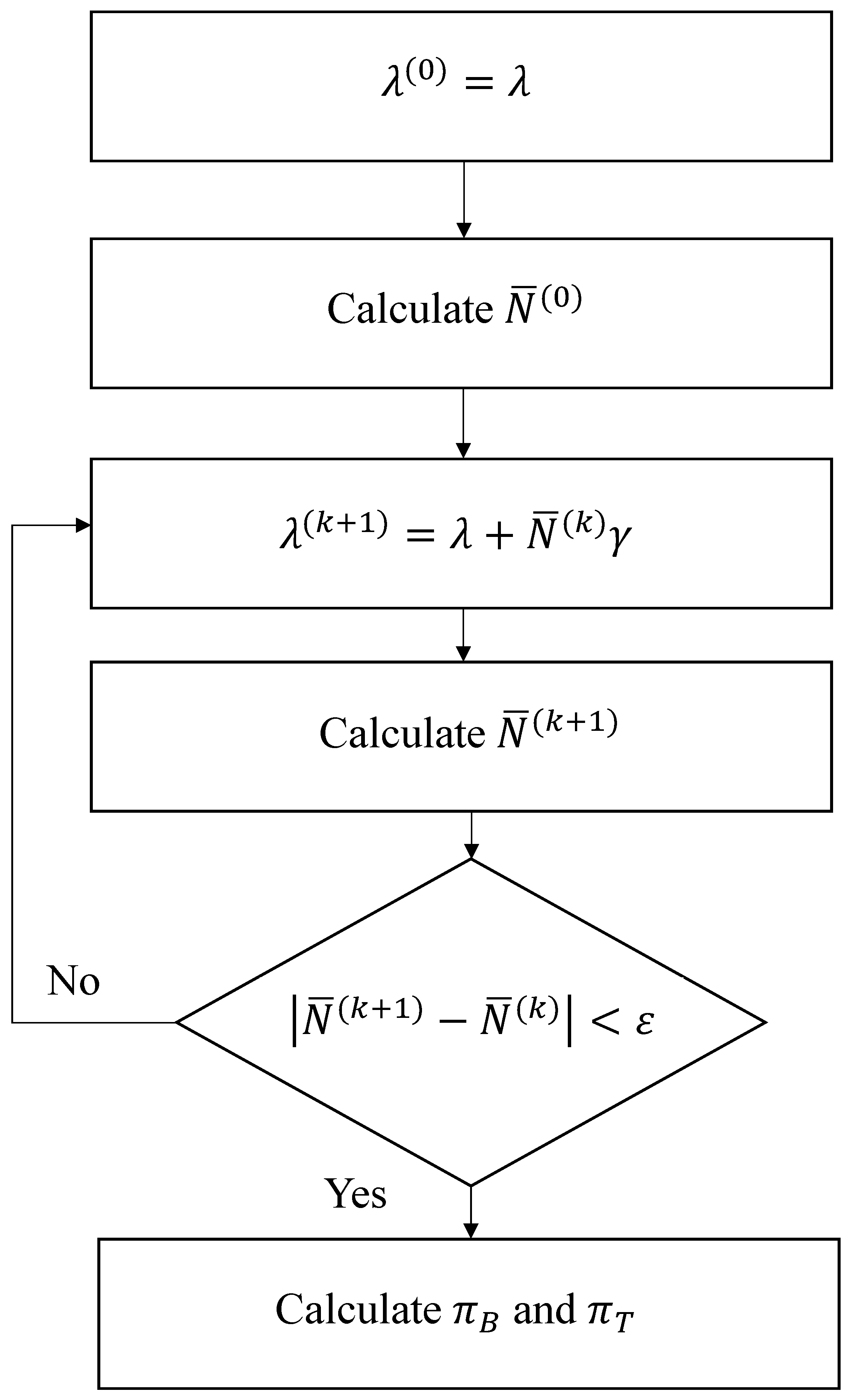
3.3. Iterative Algorithm

Once the distribution of the Markov chain embedded at departure epochs is determined, we can obtain the loss probability of secondary customers, which corresponds to the probability ${\pi }_s$ that the arrival of a signal leads to the loss of a customer in the initial system, that is,

$${\pi }_s=\sum _{k=1}^{N-1}\sum _{r=0}^R{\widehat{q}}_k\left(r\right)\sum _{j=R-r+1}^R{p}_j$$

(24)

Observe that in the considered system, the loss probabilities of primary and secondary customers differ. The rate-conservation law in the stationary regime takes the following form:

$$\lambda (1-{\pi }_B)=\overline{N}\mu +\overline{N}\gamma {\pi }_s,$$

(25)

which leads to the following mean number of customers in the system

$$\overline{N}={\displaystyle \frac{\lambda (1-{\pi }_B)}{\mu +\gamma {\pi }_s}}.$$

(26)

The iterative procedure starts with the zero intensity of the secondary flow, ${\lambda }^{\left(0\right)}=\lambda$. By utilizing (14), (15), (22), and (23) for the stationary distribution of the ReLS without signals, we evaluate probabilities ${\pi }_B$ and ${\pi }_s$ according to (9) and (24), respectively. The mean number of customers ${\overline{N}}^{\left(0\right)}$ in the system is then obtained using (26). Finally, we proceed to the next iteration of the procedure, with ${\lambda }^{\left(1\right)}=\lambda +{\overline{N}}^{\left(0\right)}\gamma$ to obtain the next value of the mean number of customers ${\overline{N}}^{\left(1\right)}$. The iterative procedure continues until the desired accuracy $ϵ$ is achieved, $\left|{\overline{N}}^{(k+1)}-{\overline{N}}^{\left(k\right)}\right|<ϵ$.

When a stable solution is achieved, the final values of the loss probability ${\pi }_B$ and termination probability ${\pi }_T$ are evaluated according to (11). A schematic of the proposed algorithm is shown in Figure 3.

4. Numerical Results

In this section, we compare the accuracies of previously developed and new approximation methods. The comparison is based on the exact numerical solution of balance Equations (6)–(8). Relative error was used as a metric for comparison.

Two sets of initial parameters were used for numerical analysis. In the first artificial case, we assumed $N=100$ servers, $R=100$ resource units, and the service intensity $\mu =1$. The resource requirement distribution is assumed to follow a truncated geometric distribution with parameter $p=0.2$, that is,

$$p_j={\displaystyle \frac{(1-p)p^{j-1}}{1-p^R}}, 1\le j\le R.$$

(27)

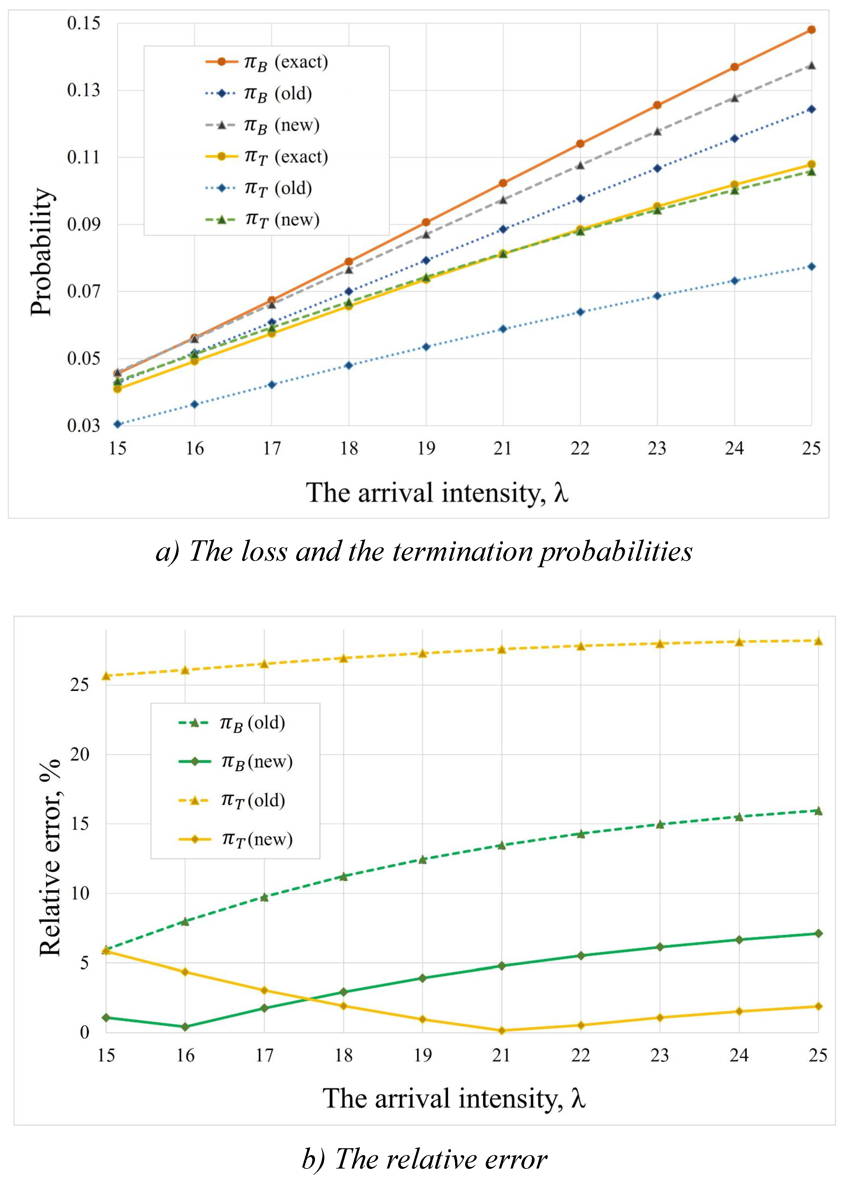
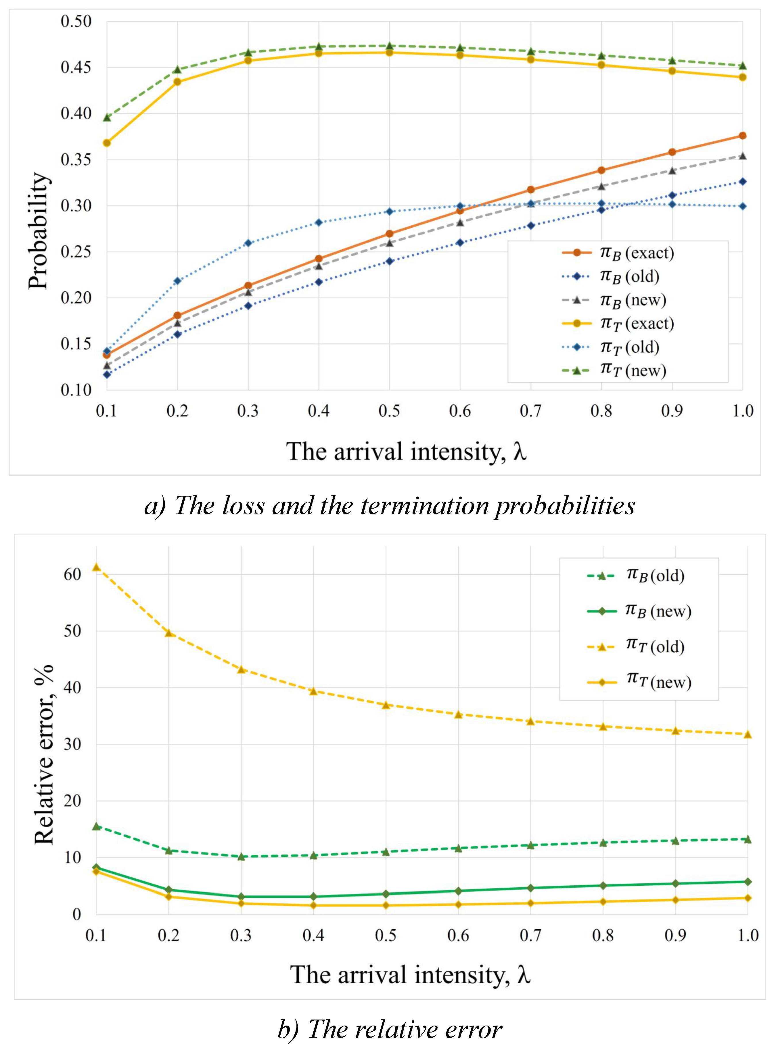
In Figure 4, we set the signal arrival intensity $\gamma =2$, and analyzed the accuracy of the main probabilistic measures for various values of the arrival intensity $\lambda$. Figure 4a illustrates the values of the loss and termination probabilities, ${\pi }_B$ and ${\pi }_T$, respectively, obtained using three different methods: numerical solution of balance equations (labeled with “exact”), the approximation method proposed in [15] (labeled with “old”), and the new approximation developed in this paper (labeled with “new”). Figure 4b illustrates the relative errors of both the approximation methods. It is evident that the relative error of the old approximation method for the evaluation of the termination probability is unacceptably large, even under low-load conditions (over 25%). The relative error of this method for the loss probability resulted in a significantly smaller relative error of approximately 5% for low-load conditions, but also increases considerably as the intensity increases (almost 15%). At the same time, the relative errors for both probabilities obtained by the new approximation method were less than 7% irrespective of the load conditions.

The evaluation of accuracy of the proposed approximation approach for some other values of $\gamma$ is given in

Table 1. Relative error of the loss probability evaluation, $\gamma =0.5$.

$\mathsf{\lambda }$	15	16	17	18	19	20	21	22	23
${\pi }_B$ (exact)	0.0528	0.0644	0.0766	0.0892	0.1021	0.1151	0.1281	0.141	0.1538
${\pi }_B$ (appr.)	0.0525	0.0636	0.0752	0.0871	0.0992	0.1113	0.1234	0.1354	0.1472
Rel. err. %	0.5	1.2	1.8	2.4	2.9	3.3	3.7	4.0	4.3
${\pi }_T$ (exact)	0.0125	0.0149	0.0174	0.0199	0.0224	0.0247	0.0271	0.0293	0.0315
${\pi }_T$ (appr.)	0.0126	0.015	0.0174	0.0198	0.0221	0.0244	0.0266	0.0288	0.0308
Rel. err. %	1.2	0.6	0.03	0.5	1.0	1.4	1.7	1.9	2.1

and

Table 2. Relative error of the loss probability evaluation, $\gamma =5$.

$\mathsf{\lambda }$	15	16	17	18	19	20	21	22	23
${\pi }_B$ (exact)	0.0372	0.0446	0.0522	0.0599	0.0678	0.0757	0.0836	0.0914	0.0992
${\pi }_B$ (appr.)	0.0386	0.0454	0.0524	0.0594	0.0664	0.0734	0.0803	0.0872	0.0939
Rel. err. %	3.7	2.0	0.5	0.9	2.0	3.0	3.9	4.7	5.4
${\pi }_T$ (exact)	0.0785	0.0913	0.104	0.1164	0.1283	0.1398	0.1507	0.1611	0.1708
${\pi }_T$ (appr.)	0.0877	0.1004	0.1126	0.1244	0.1356	0.1462	0.1657	0.1747	0.183
Rel. err. %	11.7	9.9	8.3	6.9	5.7	4.6	3.7	2.9	2.2

. We considered low signal arrival intensity $\gamma =0.5$ and high signal arrival intensity $\gamma =5$ (five signals arrive during the service time on average). Comparing the results in these tables, we can see that the accuracy of calculating the loss probability does not depend on the arrival intensity of signals. However, there is a significant increase in the relative error when calculating the termination probability for large values of $\gamma$. This effect becomes more pronounced at low-load conditions, where both probabilities are small.

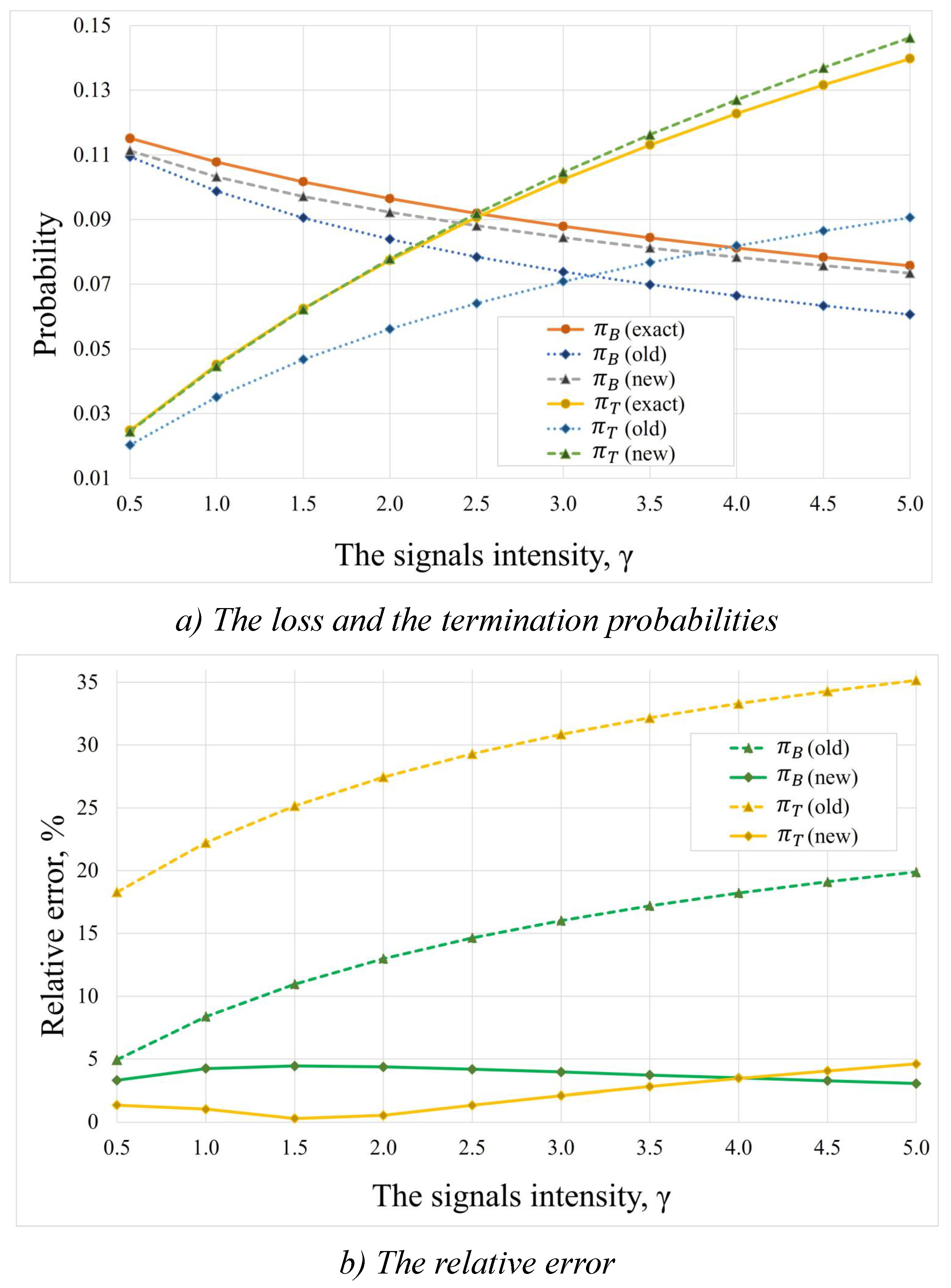
Figure 5 presents the dependence of the loss and termination probabilities on the intensity of the signal arrivals under an arrival intensity $\lambda =20$. Specifically, Figure 5a shows the absolute values of the loss and termination probabilities. It can be observed that there is an inverse relationship between the loss and termination probabilities under these conditions. This phenomenon can be explained by the fact that, as the intensity of the signal increases, so does the frequency of service terminations, resulting in an increase in the fraction of unoccupied resource units. Consequently, the probability of loss of newly arriving customers decreases. Figure 5b shows the relative errors when using these approximation methods. Both methods exhibited better values at low loads, but as the signal intensity increased, the old approximation method showed even worse accuracy than that in Figure 4b. In contrast, the new approximation method shows better values than those in Figure 4b, that is, the relative error does not exceed 5%.

Table 3. Relative error of the loss probability evaluation, $\lambda =15$.

$\mathsf{\gamma }$	0.1	0.5	1	1.5	2	2.5	3	3.5	4
${\pi }_B$ (exact)	0.0556	0.0528	0.0499	0.0476	0.0455	0.0437	0.0422	0.0407	0.0395
${\pi }_B$ (appr.)	0.0555	0.0525	0.0499	0.0478	0.046	0.0445	0.0431	0.0418	0.0407
Rel. err. %	0.3	0.5	0.1	0.5	1.1	1.6	2.1	2.6	3.0
${\pi }_T$ (exact)	0.0027	0.0125	0.0232	0.0326	0.0409	0.0485	0.0555	0.0619	0.0678
${\pi }_T$ (appr.)	0.0027	0.0126	0.0238	0.034	0.0433	0.052	0.06	0.0676	0.0747
Rel. err. %	0.1	1.2	2.8	4.4	5.8	7.1	8.2	9.3	10.2

and

Table 4. Relative error of the loss probability evaluation, $\lambda =25$.

$\mathsf{\gamma }$	0.1	0.5	1	1.5	2	2.5	3	3.5	4
${\pi }_B$ (exact)	0.19	0.1786	0.1666	0.1566	0.148	0.1406	0.1342	0.1284	0.1233
${\pi }_B$ (appr.)	0.1873	0.1702	0.1561	0.1458	0.1375	0.1306	0.1247	0.1195	0.1149
Rel. err. %	1.4	4.7	6.3	6.9	7.1	7.1	7.0	6.9	6.8
${\pi }_T$ (exact)	0.0078	0.0354	0.0639	0.0877	0.1079	0.1254	0.1409	0.1547	0.1671
${\pi }_T$ (appr.)	0.0077	0.0346	0.0622	0.0856	0.1058	0.1238	0.1398	0.1543	0.1676
Rel. err. %	0.8	2.4	2.7	2.4	1.9	1.3	0.8	0.2	0.2

present the results of accuracy evaluation with different values of the customer arrival rate $\lambda$. The values in Table 3 correspond to low-load conditions ($\lambda =15$), while Table 4 represents high load ($\lambda =25$). Comparing the two tables, we can see that there is a similar trend: with a low customer arrival intensity (${\pi }_B<0.05$) and high signal arrival intensity $\gamma$, the relative error of the termination probability evaluation begins to increase significantly. This is because with a low customer arrival rate and a high signal arrival rate, the “weight” of the flow of secondary customers triggered by signals becomes larger relative to the flow of primary customers. Therefore, the higher the relative weight of secondary customer flow, the greater the relative error introduced by our approximation method.

Next, we considered a slightly different set of initial data. The parameter of geometric distribution for resource requirements is $p=0.4$, and the customer arrival intensity $\lambda =40$. The results of the accuracy evaluation of the proposed method for various signal intensity values are presented in

Table 5. Relative error of the loss probability evaluation, $\lambda =40$.

$\mathsf{\gamma }$	0.1	0.5	1	1.5	2	2.5	3	3.5	4
${\pi }_B$ (exact)	0.0925	0.0866	0.0806	0.0756	0.0714	0.0678	0.0646	0.0618	0.0592
${\pi }_B$ (appr.)	0.0912	0.0831	0.0766	0.0719	0.0681	0.065	0.0622	0.0598	0.0577
Rel. err. %	1.4	4.1	5.0	5.0	4.6	4.2	3.6	3.1	2.6
${\pi }_T$ (exact)	0.0035	0.016	0.0292	0.0406	0.0505	0.0593	0.0671	0.0742	0.0807
${\pi }_T$ (appr.)	0.0034	0.0155	0.0285	0.038	0.05	0.0592	0.0677	0.0755	0.0828
Rel. err. %	1.0	2.7	2.7	2.0	1.1	0.1	0.8	1.7	2.5

.

In Figure 6 and Figure 7, we utilize a set of initial data from [13] for the performance evaluation of a 5G New Radio (NR) BS with user session data rates of 5 Mbps bitrate. We consider a system with $N=70$ servers representing signal processors and $R=70$ resource units corresponding to the primary resource blocks (PRBs). The session service time was exponentially distributed, with $\mu =1/30$ s. The distribution of resource requirements was calculated by considering the location of the user and the variation in signal quality, as discussed in [13] and presented in

Table 6. Resource requirements distribution of the second dataset.

Resource units	3	4	5	6	8	10
Probability	0.101	0.082	0.058	0.143	0.092	0.086
Resource units	12	16	24	37	60	70
Probability	0.093	0.086	0.083	0.072	0.06	0.044

. Here, signals model session interruptions caused by the blockage of the line-of-sight (LoS) propagation path between users and the BS.

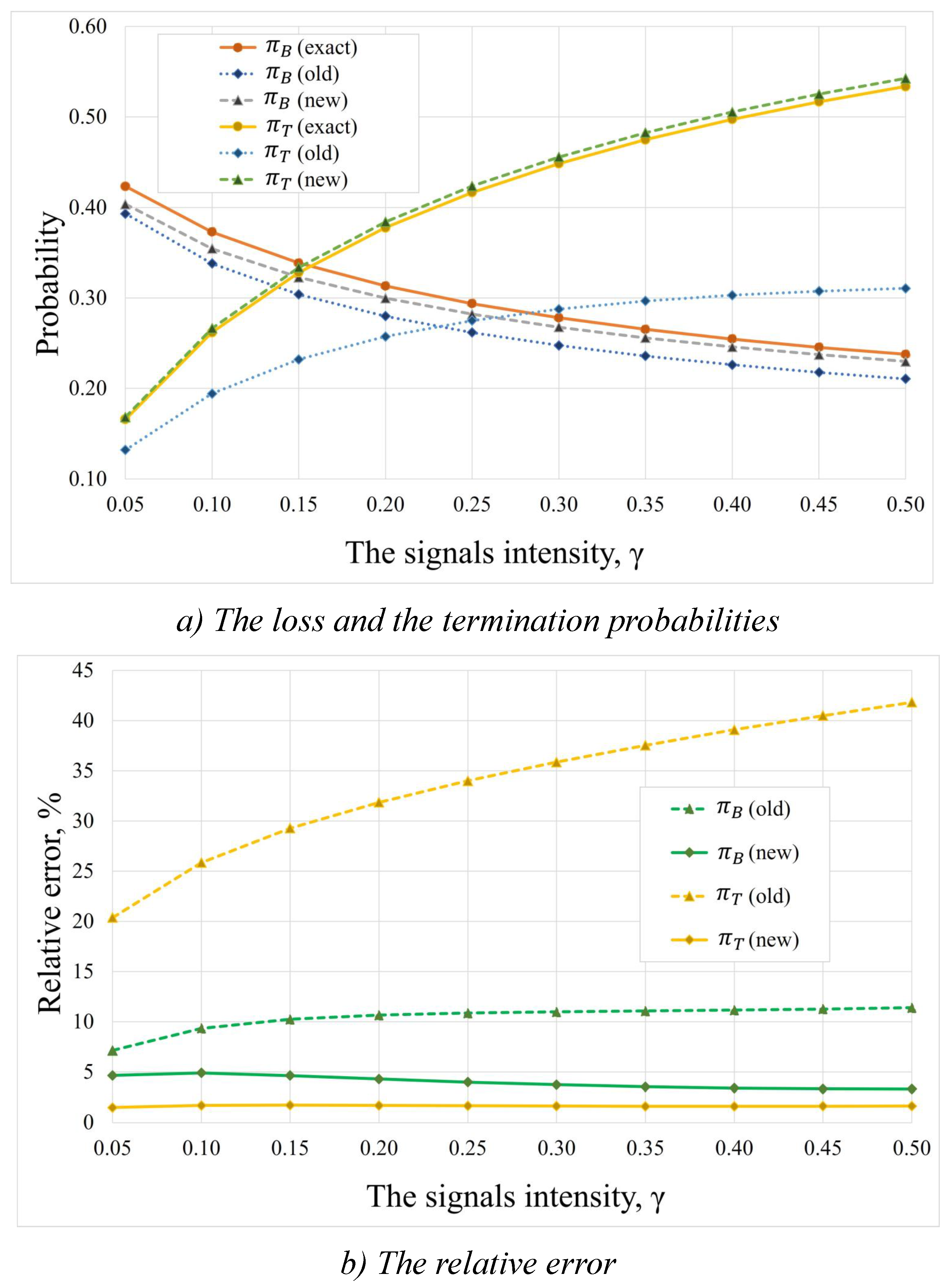
Figure 6 shows the results obtained for $\gamma =0.33$, which roughly correspond to the conditions of a large crowd. Figure 6a illustrates the dependence of the loss and termination probabilities on the arrival intensity, while Figure 6b shows the relative error of the approximation methods. The results did not change significantly for the second dataset. The relative errors of the old approximate method are much larger. The relative error of the termination probability never fell below 30% and the relative error of the loss probability was greater than 10%. For the proposed approximation method, the relative error never exceeded 10%.

The results for different arrival intensities $\lambda =0.5$ are shown in Figure 7, where Figure 7a presents the dependence of the loss and termination probabilities on the signal intensity, while Figure 7b illustrates the relative error of the approximation methods. The old approximation method showed an acceptable accuracy for the loss probability. However, the relative error of the termination probability was still far from acceptable. The new approximation method shows much better performance for both the loss and termination probabilities, where the relative errors always remain below 5%.

5. Conclusions

Queuing systems with random resource requirements and signals are useful tools for modeling the performance of modern cellular systems. Motivated by the lack of an analytical solution for this class of systems, in this study, we propose an improved method for analytical approximation of probabilistic characteristics. The proposed approach is based on the use of approximating systems without signals and additional flow of customers and precise characterization of the rate of interrupted customers based on the stationary probabilities of the Markov chain embedded in the departure epochs. This distribution was used instead of the process distribution to calculate the termination probability.

As a result, the improvement of the main approximation idea leads to a much higher accuracy of the calculations. The accuracy of the proposed approach was evaluated by comparing its results with those of an exact numerical solution. The numerical results show that the proposed approximation method is characterized by a relative error of approximately 5–10% over a wide range of system parameters and load conditions.

As part of our future research in this field, we plan to develop an efficient computational algorithm that is similar to the one presented in [22], and supplement it with the evaluation of the termination probability.