Microeconomic Shock Propagation Through Production Networks in China

Abstract

The question of whether microeconomic shocks induce aggregate fluctuations constitutes a central issue in economic research. This paper introduces a general equilibrium model with production networks to explore the propagation mechanisms of microeconomic shocks. A novel triangular production network structure is introduced, and simulations are performed using China’s input-output table to analyze the propagation of these shocks within the Chinese economy. The model demonstrates that the first-order effects of microeconomic shocks propagate downstream along the industrial chain, while the second-order effects of microeconomic productivity shocks propagate both upstream and downstream along the chain. The first-order propagation mechanism of microeconomic shocks involves changes in prices within the affected sector and its downstream sectors. Additionally, the second-order effects of microeconomic shocks rely on the reallocation of factors. The simulation results indicate that China’s production network matrix is triangular, and that the financial sector plays a crucial role in amplifying the effects of microeconomic shocks. Government should prioritize supporting upstream fundamental sectors to mitigate the adverse impacts of external shocks on economic fluctuations and to address systemic financial risks.

1. Introduction

The question of whether microeconomic idiosyncratic shocks lead to aggregate fluctuations and how these shocks propagate through intersectoral input-output linkages has been a central issue in economic research. Microeconomic shocks refer to events or disturbances that affect individual agents or sectors at a micro level, while aggregate fluctuations represent changes at the aggregate level of a country or region. The understanding that the production of goods and services depends on a complex network of transactions among suppliers and consumers has a well-established foundation in economic theory [1]. As early as 1941, Leontief observed that “Layman and professional economist alike, practical planner and the subjects of his regulative activities, all are equally aware of the existence of some kind of interconnection between even the remotest parts of a national economy” [2]. As the production process becomes more and more specialized, this connection deepens and expands, forming a complex network system among diverse production units within economic entities. In this network, each firm or sector purchases intermediate inputs from upstream suppliers, while supplying intermediate products to downstream buyers. This interdependent system, known as the “production network”, reflects nature of input-output linkages.

When studying issues of macroeconomic fluctuations, economists typically adopt a macro-level perspective. For example, the Keynesian school and the monetarist school focus respectively on analyzing insufficient aggregate demand and fluctuations in the aggregate money supply. However, this argument neglects the input-output linkages between firms or sectors, thereby failing to delve into the microeconomic foundations of macroeconomic fluctuations. Existing research overlooks micro-level details for two primary reasons. First, Lucas’s “diversification argument” posits that production diversification effectively reduces macroeconomic volatility, averaging out the aggregate impact of microeconomic shocks to an inconsequential level [3]. Second, Hulten’s theorem suggests that in an efficient economy, the macroeconomic effects of microeconomic shocks can be encapsulated through sales shares [4]. Thus, microeconomic details, such as the structure of production networks, are often regarded as merely indirect factors influencing aggregate fluctuations. Such perspectives appear to have diminished the perceived research significance of production networks. However, the 2008 financial crisis, originating in a specific industry within a single country and subsequently spreading globally, reignited interest in firm-level and sectoral shocks within both academic and industry circles. According to traditional views, the effects of micro-level shocks are typically “smoothed out” during propagation, with their influence constrained by the output share of sectors or the sales share of firms. However, this perspective is evidently inconsistent with the realities of the financial crisis. Therefore, new theories are urgently needed to explain the formation of aggregate fluctuations.

A strand of literature, beginning with works such as Gabaix [5], Jones [6], and Acemoglu et al. [7], has incorporated financial networks, input-output networks, or production networks into analytical frameworks to explore how localized shocks propagate to other firms or sectors, thereby triggering systemic crises. This body of literature fundamentally challenges Lucas’s view on the negligible impact of local shocks and expands on Hulten’s theorem. First, when considering production networks, firms or sectors highly rely on the inputs and outputs of other firms or sectors, thereby challenging Lucas’s assumption of independent shocks. Second, when the distribution of firm or sector sizes is heavy-tailed, the Law of Large Numbers, which underpins Lucas’s theory, no longer holds. In such cases, localized shocks in key firms or sectors can trigger systemic crises [7]. Third, the introduction of higher-order or distortionary effects renders Hulten’s theorem inapplicable, allowing the production network to influence the overall impact of microeconomic shocks [8]. In light of these considerations, macroeconomic fluctuations constitute the most direct application of production network analysis. The propagation of microeconomic productivity shocks can be systematically examined through both supply-side and demand-side channels. From the demand perspective, since the production of any single firm or sector in the production network requires intermediate inputs from other firms or sectors, changes in output or structure caused by microeconomic shocks will lead to changes in the demand for intermediate inputs by the directly affected firm or industry, thereby propagating the impact of the shock to upstream microeconomic agents. From the supply perspective, the products of any economic entity also serve as raw materials for downstream firms or sectors. When a directly affected firm or sector in the upstream halts supply for an extended period, downstream firms or sectors will face supply shortages, thus transmitting the impact of the microeconomic shock to downstream microeconomic agents. Therefore, microeconomic shocks inevitably propagate through production networks shaped by input-output linkages, ultimately leading to macroeconomic effects.

Beyond the domain of macroeconomics, the production network approach has been widely applied in areas such as regional trade, financial crises, and supply chain resilience. In the domain of regional trade, studies explore network linkages among firms to assess how exogenous shocks and trade policies shape domestic economies, including export demand shocks [9] and the entry of foreign firms [10]. Some research adopts a spatial equilibrium framework, examining the endogenous formation of production networks and their welfare implications [11]. In the context of financial crises, studies investigate how shocks originating in a single country’s financial sector propagate through international production networks to other open economies [12] and how such shocks spread domestically via trade and credit networks [13]. The extent of financial contagion is determined not only by the structure of production networks but also by the magnitude of financial shocks [14]. Regarding supply chain resilience, research analyzes the macroeconomic consequences of exogenous shocks that disrupt supply chains [15], offering insights into policies designed to enhance supply chain robustness. While firm failures and subsequent supply chain disruptions can exacerbate the adverse impacts of shocks [16], firms facing supply chain risks may strategically reconfigure inter-firm production networks to reduce reliance on unstable suppliers [17].

Based on the above research, this paper seeks to explore the network origins of aggregate fluctuations from four perspectives: What is the direction of propagation of microeconomic shocks through industrial chains? What is the mechanism of shock propagation through the production network? What role does the structure of the production network play in this propagation process? And how can industrial policies be designed based on the structure of production networks? To address the above questions, this paper first analyzes in detail the upstream and downstream propagation mechanisms of microeconomic shocks. However, due to the complexity of production networks, the magnitude and direction of the role played by them remain ambiguous, especially when considering more general Constant Elasticity of Substitution (CES) substitution elasticities. In this context, simplifying the propagation of microeconomic shocks based on the structure of the actual production network becomes advantageous for obtaining tractable analytical results. Fortunately, the triangular production network, which has been validated in empirical data and the literature, provides a basis for assessing the impacts of microeconomic shocks. Subsequently, this paper integrates the nonlinear effects of microeconomic shocks into the analysis. The direct impact of microeconomic shocks on macroeconomic variables is referred to as the first-order effect, while the influence of these shocks on the first-order effects is termed the second-order effect. Theoretically, this approach conceptualizes macroeconomic variables as a function of microeconomic shocks. By performing a second-order Taylor expansion of this function around the equilibrium point, one can separately derive the variable’s mean, the first-order effects, and the second-order effects. Finally, this paper applies the model to conduct numerical simulations based on China’s 2018 input-output table. The analysis verifies the triangular structure of China’s input-output linkages and then performs simulations of first- and second-order propagation. These simulations are utilized to examine the characteristics of the production network and the mechanisms of shock propagation. Based on this analysis, the paper clarifies the direction, mechanism, and outcomes of shock propagation, as well as the role played by the production network, providing a reference for fully understanding the crucial role of the financial sector.

This study makes the following three major contributions. First, by constructing a general equilibrium model framework that incorporates the production network structure, this paper offers a thorough exploration and analysis of the propagation mechanism of microeconomic shocks along both the upstream and downstream segments of the industrial chain, highlighting the critical role of the production network structure in this process. Second, to facilitate the development of the theoretical model and the implementation of numerical experiments, this study introduces a specific production network structure as a research tool. Compared to previous models, this paper employs the triangular production network structure observed in real-world data to simplify the upstream and downstream transmission of shocks, thereby unveiling the black box of production network effects. Finally, this paper utilizes China‘s production network structure to simulate the first- and second-order effects of microeconomic shocks, with a detailed exploration of the micro-level factors that influence the direction or magnitude of these effects. These findings not only contribute to the enrichment of the theoretical framework but also offer actionable insights for policymakers.

The rest of the paper is organized as follows. Section 2 reviews the literature on microeconomic shocks and production networks; Section 3 presents the theoretical framework of the paper; Section 4 derives the main results on the propagation of microeconomic shocks; Section 5 conducts simulations using China’s input-output data; and Section 6 concludes and discusses.

2. Literature Review

This paper presents a review of the propagation of microeconomic shocks through production networks, focusing on the structural characteristics of production networks, general equilibrium models incorporating production networks, and the applications of production network methodologies.

2.1. Characteristics of Production Networks

Understanding the structural characteristics of production networks is the starting point for examining the propagation of microeconomic shocks from a production network perspective. The existing literature summarizes three key structural characteristics of production networks: (1) Production networks exhibit asymmetry, evidenced by the fact that a small number of sectors function as critical suppliers to all other sectors of the economy [7]. In economies where a few dominant sectors prevail, as is the case in the United States, shocks to these sectors are transmitted throughout the entire economic system; (2) Production networks are characterized by low link density yet high connectivity, as evidenced by a limited number of links and short average distances between sectors [15]; and (3) Production networks at the firm level exhibit greater structural heterogeneity compared to those at the sectoral level [18].

Asymmetry is a crucial characteristic in the development of shock propagation theory from the production network perspective. Horvath [19,20] contends that different sectors assume distinct roles in the input-output relationship, with a small number of core sectors supplying intermediate inputs to most industries. This results in the fact that specific shocks occurring in the dominant sector are harder to offset by reverse shocks in other sectors. Dupor [21] investigates how different input-output relationships influence fluctuations in aggregate output across various multisectoral models. He finds that when the variance of the input-output matrix is relatively low, indicating a more balanced distribution of sectoral linkages, the overall propagation effect of sectoral shocks is limited. Acemoglu et al. [7] argues that there are influence vectors in the economic system, which give rise to an “axis-periphery” type of asymmetry in the structure of the production network. This asymmetry ultimately reduces the rate of attenuation of fluctuations in aggregate output due to micro shocks. Therefore, to study the specific role of production networks in microeconomic shocks, it is crucial to leverage the asymmetric structures inherent in these networks.

To investigate domestic changes in industrial structures and facilitate international comparisons, the triangular or hierarchical structure emerges as a highly effective analytical tool. The production network matrix is usually sparse because a few key sectors in the production network supply the majority of sectors. Based on this property, the production network can be reorganized in such a way that the matrix is transformed into a triangular form. This idea dates back to the 1950s, when Chenery and Watanabe [22] found a similar hierarchical structure by comparing input-output matrices in the United States, Japan, Norway, and Italy. Simpson and Tsukui [23] first proposed an algorithm for concentrating the larger elements of the matrix by reordering the sectors into a corner. Subsequently, Fukui [24] further enhanced the rationality and scalability of this algorithm, and demonstrated that similar triangular structures exist in both more developed countries (the United States, Italy, Norway, and Japan) and less developed countries (Korea and India). With the aid of modern visualization tools, these triangular matrix structures can now be clearly illustrated, as shown in studies on Japan [25], Korea [26], and China [26]. This approach not only enhances the interpretability of production networks and highlights inter-sectoral dependencies but also significantly simplifies the computation of systems of linear equations [27].

2.2. General Equilibrium Model with Production Networks

In the literature examining the microeconomic origins of aggregate fluctuations, the starting point is the fundamental theorem proposed by Hulten: for efficient economies, the effect of microeconomic total factor productivity (TFP) shocks on aggregate TFP is equal to the sales share in GDP of the affected sectors [4]. The latter is known as the Domar weight in the literature. The corollary of Hulten’s theorem is that, in the presence of input-output linkages, the impact of a microeconomic shock on the outcome of an aggregate shock is entirely determined by the size of its sales share, regardless of its position within the production network. Therefore, economists have long downplayed the role of production networks in macroeconomic models. For example, Lucas [3] argued that, according to the law of large numbers, the effects of shocks in a single sector are “ironed out” by other sectors, resulting in a negligible macroeconomic impact.

However, Hulten’s theorem faces several issues both theoretically and practically. Theoretically, (1) the Domar weight, as a statistic, only captures first-order effects, meaning that it may not provide an accurate approximation when shocks are large or when there are significant nonlinearities in the economy [8]; (2) Hulten’s theorem holds true only in an efficient economy and is not applicable in the presence of frictions and market imperfections [28]. (3) While Hulten’s theorem demonstrates that the Domar weight is a sufficient statistic for measuring how microeconomic shocks affect aggregate output, these weights remain endogenous, being determined within the equilibrium of the economy [29]. In practice, sectors with the same sales share play significantly different roles in economic fluctuations, and a negative shock to one sector can potentially lead to the collapse of the entire economy. Therefore, a new theory is urgently needed to further characterize the relationship between microeconomic shocks and aggregate fluctuations.

Aggregate fluctuation theory with production network is the breakthrough point to recharacterize microeconomic shocks, and is based on multisectoral general equilibrium models. In the 1980s, Long and Plosser [30] developed a multisector real business cycle model, which serves as a valuable benchmark for evaluating the significance of various factors, such as monetary disturbances, in the real business cycle. In the 1990s, this model was further developed, with debates between Horvath [19,20] and Dupor [21] focusing on whether sectoral shocks translate into macroeconomic fluctuations. However, after a prolonged period, the development of aggregate fluctuation theory, including networks, stagnated due to the lack of suitable analytical tools. Until recently, with advancements in network theory and the innovation of analytical tools, the connections between each production unit in a production network could be defined and measured, making it possible to explore how microeconomic shocks propagate throughout the economy. Acemoglu et al. [7] proposed a general static analytical framework that incorporates input-output linkages into the propagation mechanism of heterogeneous shocks, thereby providing a microeconomic explanation for aggregate fluctuations. The significant difference between this model and traditional models is that traditional models assume intermediate goods are produced solely by primary factors and then combined into final products by an “aggregated sector”. In contrast, the production network model emphasizes the correlation and interaction between sectors through input-output linkages. Since then, the analytical framework has been refined and expanded to provide a more realistic picture of the real economy.

Specifically, the relevant literature has made the following theoretical contributions. The first contribution is to reveal the microeconomic roots of macroeconomic fluctuations from the perspective of production networks. Acemoglu et al. [7] examined a static multisector economic system within a perfect competition framework and Cobb–Douglas technology to explore the origins of aggregate fluctuations. Baqaee and Farhi [8] further characterized the nonlinear macroeconomic effects of microeconomic shocks. Their results suggest that asymmetry is a crucial factor that enables the structure of production networks to play a significant role. Second, recent research has further explored the propagation mechanism of microeconomic shocks. Acemoglu et al. [16] analyze the direction of propagation of microeconomic shocks within a Cobb–Douglas technology setting. They find that productivity shocks are transmitted downstream, from the source to its downstream customers, and to the customers of those customers, and so on. In contrast, demand shocks are transmitted upstream, from the source to its suppliers, and to the suppliers of those suppliers. Carvalho et al. [15] introduce nested CES structures in production functions and show that when the elasticity of substitution between various intermediate inputs or between intermediate products and primary input factors is different from 1, the productivity shock to a specific sector will affect the output of other sectors through the two different channels. Third, general equilibrium models incorporating production networks provide critical insights into economic development and policy design. Baqaee and Farhi [31] extend the framework to include Heterogeneous Agents and Input-Output Networks (HA-IO) linking various economic issues such as sectoral linkages in business cycles, factor-biased technological change, and the fiscal multiplier’s dependence on government spending composition. Liu [26] argues that market imperfections within production networks lead to distortion effects, which are further intensified by reverse demand linkages. As a result, the most significant distortions occur in upstream sectors, indicating that effective industrial policies should subsidize these sectors.

2.3. Empirical Studies of Production Networks

Building on the framework of models with production network structures, the relevant literature has conducted empirical analyses of the propagation mechanisms and directions of microeconomic shocks. Acemoglu et al. [16] were the first to empirically test the shock propagation mechanisms and directions predicted by the benchmark model at the sectoral level. Their findings reveal that the downstream network effects of productivity shocks are both economically and statistically significant: a one standard deviation increase in sectoral TFP results in a 6% growth in downstream output. Barrot and Sauvagnat [18], on the other hand, utilize firm-level data to investigate the localized propagation patterns of specific natural disaster shocks (e.g., blizzards, earthquakes, floods, and hurricanes) across firms’ production networks. Their findings indicate that the sales growth rate of direct customers of affected firms decreases by 2–3 percentage points. Boehm et al. [32] and Carvalho et al. [15] identified a similar propagation pattern while examining the impact of the 2011 earthquake and tsunami on production networks in Japan. Furthermore, the existing literature has measured the volatility caused by oil shocks [33], financial shocks [13], and the COVID-19 pandemic [34] within the production network framework, as well as the specific effects of monetary policy [35], fiscal policy [36], and industrial policy [26] on aggregate output and welfare.

In summary, from the modeling framework proposed by Acemoglu, numerous studies have extended the general equilibrium model incorporating the structure of the production network. These extensions include the introduction of general constant elasticity of substitution (CES) nested functions [15,31], the incorporation of market incompleteness [26,28], and the endogenization of the production network [29,37]. These models have been further tested through empirical analysis and numerical simulations.

However, the studies mentioned above do not explore in depth the propagation mechanisms of the first- and second-order effects of micro shocks, nor do they analyze the interconnections between upstream and downstream sectors through the triangular input-output structure. Additionally, they do not go beyond disaggregating the first- and second-order effects to clarify the magnitude of the production network’s impact. Therefore, this paper examines the structural effects of productivity shocks at the sectoral level by incorporating the triangular production network structure into the model, delineating the propagation mechanisms of these shocks within the input-output network, and ultimately offering new insights for theoretical research and policy practice.

3. General Framework

3.1. Setup

This subsection presents a detailed description of a general equilibrium model that incorporates production networks, following the “CES standard form” as defined by Baqaee and Farhi [8]. The model considers a perfectly competitive economy with $N$ production sectors and $M$ factor sectors and assumes the presence of a representative household. Without loss of generality, we interchangeably use italic symbols to represent scalars, vectors, and matrices. Additionally, overlined symbols indicate the equilibrium value of the variable and are used to normalize the variable.

We first assume the pure sectoral assumption, meaning that each sector produces only one product. The production technology of the competitive sector $i$ is given by:

$$y_i=z_i{F}_i\left(x_{i1},x_{i2},\dots ,x_{iN},f_{i1},f_{i2},\dots ,f_{iM}\right),$$

(1)

where $y_i$ denotes the output of sector $i$, $z_i$ denotes total factor productivity (TFP), $x_{ij}$ denotes the intermediate inputs from sector $j$ used in sector $i$ (intermediate inputs), and $f_{ik}$ denotes the factor $k$ used in sector $i$ (primary inputs). The production function $F_i(·)$ is homogeneous of degree 1. Specially, the production equation for each sector takes the form of the constant elasticity of substitution (CES), i.e.:

$${\displaystyle \frac{y_i}{\overline{y_i}}}=z_i{\left({\displaystyle \sum }_{j=1}^N{a}_{ij}{\left({\displaystyle \frac{x_{ij}}{\overline{x_{ij}}}}\right)}^{{\displaystyle \frac{{\theta }_i-1}{{\theta }_i}}}+{\displaystyle \sum }_{k=1}^M{\alpha }_{ik}{\left({\displaystyle \frac{f_{ik}}{\overline{f_{ik}}}}\right)}^{{\displaystyle \frac{{\theta }_i-1}{{\theta }_i}}}\right)}^{{\displaystyle \frac{{\theta }_i}{{\theta }_i-1}}},$$

(2)

where $z_i$ denotes the Hicks-neutral productivity of sector $i$ and $\log z_i$ is usually used to denote productivity shocks. $a_{ij}$ and ${\alpha }_{ik}$ denote the size of intermediate and primary inputs, respectively, and ${\theta }_i$ represent the elasticity of substitution in sector $i$.

The competitive manufacturer maximizes its profit, which is given by the following objective:

$$\underset{x_{ij},f_{ik}}{\max }\left(p_i{y}_i-{\displaystyle \sum }_{j=1}^N{p}_j{x}_{ij}-{\displaystyle \sum }_{k=1}^M{w}_k{f}_{ik}\right),$$

(3)

where $p_i$ represent the price of the output from sector $i$ and $w_k$ represent the wage rate or price of the factor $k$. When the production function is homogeneous of degree one, the profit maximization problem results in zero profit for the efficient economy. This implies that the value of output is entirely distributed as income to the factors of production, in proportion to their respective shares.

The final demand $Y$ of a household is expressed as a function of the demand for each sector, which can be represented as:

$$Y=\underset{c_1,c_2,\dots ,c_N}{\mathit{max}}D\left(c_1,c_2,\dots ,c_N\right),$$

(4)

where $c_i$ denotes the household’s final demand for sector $i$, and the function $D(·)$ is homogeneous of degree 1. Specifically, final demand can be expressed as the CES aggregation of demand for each sector, that is:

$$Y={\displaystyle \frac{y_0}{\overline{y_0}}}={\left({\displaystyle \sum }_{j=1}^N{a}_{0j}{\left({\displaystyle \frac{c_j}{\overline{c_j}}}\right)}^{{\displaystyle \frac{{\theta }_0-1}{{\theta }_0}}}\right)}^{{\displaystyle \frac{{\theta }_0}{{\theta }_0-1}}},$$

(5)

where $a_{0j}$ denotes the share of final demand in each sector and ${\theta }_0$ represents the elasticity of substitution in consumption. It is assumed that no technological shocks occur in the final demand sector, implying that $z_0=0$.

Next, we describe the general equilibrium. The output of goods (supply) is allocated across each sector and to the final product (demand). Thus, the clearing condition for the product market is that, for each $1\le i\le N$, there is:

$$y_i={\displaystyle \sum }_{j=1}^N{x}_{ji}+c_i.$$

(6)

It is assumed that the quantity of each factor is exogenously given (supply) and allocated across each sector (demand). Thus, the clearing condition for the factor market is that, for each $1\le k\le M$, there is:

$${\displaystyle \sum }_{i=1}^N{f}_{ik}=f_k=\overline{f_k}.$$

(7)

General equilibrium necessitates three conditions: the maximization of profits in the production sector, the maximization of output in the final demand sector, and the clearing of both good and factor markets. This means that given a vector of productivity shocks and a vector of factors, a series of prices, a vector of final demand, a vector of output, a matrix of intermediate inputs, and a matrix of primary inputs can be solved. Final demand can be expressed as a function of productivity shocks and primary inputs, that is:

$$Y=f\left(z_1,z_2,\dots ,z_N,\overline{f_1},\overline{f_2},\dots ,\overline{f_N}\right).$$

(8)

Thus, with factor exogeneity given, final demand is affected only by productivity shocks, and the magnitude of this effect depends only on the exogenous parameters and the parameters of the model.

3.2. Representation of Production Networks

The production network consists of three components: intermediate inputs (producers), primary goods (factors), and final demand (household). The first two components are aggregated to form a macroeconomy through a nested constant elasticity of substitution (CES) function. This implies that each sector acts as a generalized factor of production within the CES production function, with its own distinct elasticity of substitution. The goods of the sector are aggregated one or more times, ultimately yielding macroeconomic variables such as total output and final demand. This production network structure can be represented in two forms: graphic and matrix.

First, Figure 1 depicts the graphical form of the production network. In this directed weight graph, each node corresponds to a sector in the economy, resulting in a total of $\left(1+N+M\right)$ nodes. Each pair of nodes is connected by a generalized input-output relationship, forming a total of $\left(1+N+M\right)\times \left(1+N+M\right)$ directed links. A directed edge from node $i$ to node $j$ represents inputs from sector $i$ to sector $j$; the weight of the directed edge $a_{ij}$ is greater than zero, where $i$ is the use sector and $j$ is the supply sector. Notably, the intermediate inputs, primary goods, and final demand exhibit distinct patterns of mutual interaction. In particular, the primary goods sector has only outward directed edges, the final demand sector has only inward directed edges, and the production sector has bidirectional and self-feedback directed edges.

Next, we use tables to present the matrix form of the production network. In the $\left(1+N+M\right)\times \left(1+N+M\right)$ matrix, each row or column represents a sector.

Table 1. Production networks in physical matrix form.

	Household	Good 1	…	Good N	Factor 1	…	Factor M
Household	0	$c_1$		$c_N$	0
Good 1	0	$x_{11}$	…	$x_{1N}$	$f_{11}$	…	$f_{1M}$
…		…		…	…		…
Good N		$x_{N1}$	…	$x_{NN}$	$f_{M1}$	…	$f_{NM}$
Factor 1	0	0			0
…
Factor M
Outputs	$Y$	$y_1$	…	$y_N$	$f_1$	…	$f_M$

represents the physical form of the production network. In this table, the horizontal axis denotes the uses and the vertical axis denotes the inputs. On the one hand, the sum of the first $1+N+M$ entries in the vertical direction equals the last entry, indicating that the total input of products and factors equals total output. On the other hand, due to the differing units of measurement in the physical form, horizontal summation is not possible. The physical form of the production network effectively reflects the production processes of the production sectors and the final demand sectors, that is, $A_i{F}_i\left(x_{i1}, x_{i2},\dots ,x_{iN},f_{i1},f_{i2},\dots ,f_{iM}\right)$, $Y=\max D\left(c_1,c_2,\dots ,c_N\right)$.

Table 2. Production networks in value matrix form.

	Household	Good 1	…	Good N	Factor 1	…	Factor M	Profits	Inputs
Household	0	$c_1{p}_1$		$c_N{p}_N$	0			0	${\displaystyle \sum }_{i=1}^N{c}_i{p}_i$
Good 1	0	$x_{11}{p}_1$	…	$x_{1N}{p}_N$	$f_{11}{w}_1$	…	$f_{1M}{w}_M$	${\pi }_1$	$p_1{y}_1$
…		…		…	…		…	…	…
Good N		$x_{N1}{p}_1$	…	$x_{NN}{p}_N$	$f_{M1}{w}_1$	…	$f_{NM}{w}_M$	${\pi }_N$	$p_N{y}_N$
Factor 1	0	0			0			0	$w_1{\overline{f}}_1$
…									…
Factor M									$w_M{\overline{f}}_M$
Outputs	$PY$	$p_1{y}_1$	…	$p_N{y}_N$	$w_1{f}_1$	…	$w_M{f}_M$

shows the production network in the value form. It is assumed that the supply side of each sector offers the same price to the buyer, ensuring that each column reflects the same price. In addition to retaining the horizontal and vertical summation properties of the physical form, the production network in value form highlights a key feature: the value of total output is equal to the value of total revenue, which is the sum of intermediate vendor revenues, primary factor revenues, and profits:

$${\displaystyle \sum }_{j=1}^N{p}_j{x}_{ij}+{\displaystyle \sum }_{k=1}^M{w}_k{f}_{ik}+{\pi }_i=p_i{y}_i.$$

(9)

On the other hand, the relationship between final demand and the consumption by each sector is as follows:

$${{\displaystyle \sum }}_{i=1}^N{c}_i{p}_i=PY,$$

(10)

where represents the price of the final product. In general, the final product is taken as the numeraire, and its price is set to 1. Under this assumption, ${\displaystyle \sum }_{i=1}^N{c}_i{p}_i=Y=GDP$. Therefore, total final demand is the most important aggregate indicator in the model.

The graphical and matrix forms of production networks are equivalent. The graphical form offers a simpler conceptual framework to summarize input-output linkages, while the matrix form facilitates easier derivation and computation [1]. Moreover, since the input-output equilibrium relationship is based on the general equilibrium theory of Walras, the input-output matrix serves as an analytical tool for general equilibrium theory, encompassing production networks. However, the matrix form of the production network exhibits distinct properties compared to the input-output matrix. First, the input-output matrix primarily describes the linear relationship between production and consumption across industries, whereas the production structure and organization in the production network can be represented by any CES function (with arbitrary elasticity of substitution), without requiring the Leontief function form (which assumes an elasticity of substitution of 0). Second, input-output analysis includes open, closed, and partially closed models, while production networks predominantly employ closed models that integrate both factor production and final demand. Third, when heterogeneous consumers are not considered, final demand in the production network matrix is consolidated into a single sector, which encompasses components such as consumption, capital formation, and net exports.

Finally, we treat both the final demand sector and the primary factor sector as general production sectors, thereby standardizing the expression of the variables. For convenience, we begin labeling the rows and columns from 0. Therefore, $x_{0j},j=1,2,\dots ,N$ is equivalent to $c_i,i=1,2,\dots ,N$; $x_{ij},i=1,2,\dots ,N,j=N+1,N+2,\dots N+M$ is equivalent to $f_{ik},k=1,2,\dots ,M$; $p_i,i=N+1,N+2,\dots ,N+M$ is equivalent to $w_k,k=1,2,\dots ,M$. In this manner, we can represent the input-output linkages between sectors uniformly in terms of $x_{ij}$, the output prices of sectors uniformly in terms of $p_i$, and the outputs of sectors uniformly in terms of $y_i$.

3.3. Coefficients in Production Networks

Coefficients in the production network can be defined based on the matrix form of the production network, thereby providing an analytical tool for further analysis. First, the direct requirements coefficient based on value is defined as:

$$A_{ij}\equiv {\displaystyle \frac{p_j{x}_{ij}}{p_i{y}_i}}.$$

(11)

In this case, the definition of the direct requirements matrix in the production network is the same as that in traditional input-output analysis, except that it is the transposition of the classical matrix of direct input coefficients. The matrix element, representing the share of sector i’s expenditures using sector j’s inputs relative to sector i’s total revenue, describes the inter-sectoral technological linkages and is consistent with the empirical results obtained by Acemoglu [16].

The Leontief inverse matrix portrays both direct and indirect links between sectors, which is defined as:

$$L\equiv {(I-A)}^{-1}=I+A+A^2+\dots .$$

(12)

Define final demand share $b_i$ as the ratio of the final demand expenditures for the product $i$ as a share of GDP, which means:

$$b_i\equiv {\displaystyle \frac{p_i{c}_i}{{{\displaystyle \sum }}_{j=1}^N{p}_j{c}_j}},$$

(13)

where the sum of the final demand for all products is 1, which means ${\displaystyle \sum }_{i=1}^N{b}_i=1$.

The Domar weight $d_i$ is an essential coefficient, which is defined as the sales of sector $i$ as a share of GDP:

$$d_i\equiv {\displaystyle \frac{p_i{y}_i}{GDP}}.$$

(14)

In much of the literature, Domar weights are commonly referred to as “sales shares”. In efficient economies, Domar weights are frequently used as sectoral weights in growth accounting [38]. Domar weights are not only a measure of sector centrality in equilibrium [26] but also have an inseparable relationship with the propagation of microeconomic shocks [4], a relationship that will be examined in greater detail in the following sections. In addition, the value of total output is greater than GDP because of the presence of intermediate inputs, and thus ${\displaystyle \sum }_{i=1}^N{d}_i>1$.

For factor $k$, its Domar weight can be similarly defined as the factor income share of GDP:

$$D_k\equiv {\displaystyle \frac{w_k{f}_k}{{{\displaystyle \sum }}_{l=1}^M{w}_l{f}_l}},$$

(15)

where the sum of the factor income shares of all factors is 1, that is, ${\displaystyle \sum }_{k=1}^M{D}_k=1$.

Finally, it can be shown that Domar weights and Leontief inverse matrices are related to the final demand share as:

$$d^{\prime }=b^{\prime }L=b^{\prime }I+b^{\prime }A+b^{\prime }{A}^2+\dots ,$$

(16)

where the superscript $\prime$ is the transpose of the representer vector. This equation implies that the sales share can be decomposed into the product of the final demand share and the Leontief inverse matrix. This equation links the variables defined earlier and will play a key role in understanding the mechanism of sales share formation with the propagation mechanism of microeconomic shocks.

4. Propagation Mechanism Analysis

We further complement and extend the modeling framework of [8,28,31] to explore the propagation process of microeconomic shocks within the production network. This section attempts to answer the following questions: First, how are microeconomic shocks transmitted along the industrial chain; second, what is the propagation mechanism of microeconomic shocks; third, how does the production network contribute to the propagation; and fourth, what are the macroeconomic outcomes resulting from microeconomic shocks. Compared to the existing literature, the innovations of the model in this paper are as follows: First, this paper innovatively introduces a triangular input-output structure to conduct a detailed analysis of the upstream and downstream transmission mechanisms; second, we further decompose the first-order and second-order effects of microeconomic shocks, aiming to explore the role of the production network in the propagation of these shocks.

4.1. First-Order Propagation

4.1.1. Hulten’s Theorem and Applications

First, we explore the first-order propagation mechanism of microeconomic shocks. Based on the general equilibrium model constructed in the previous sections, it is possible to derive the first-order effects of microeconomic shocks on aggregate output in the general case.

Theorem 1

(Hulten’s Theorem). In an efficient economy, the first-order effect of a microeconomic shock on final demand is:

$${\displaystyle \frac{d\mathit{log}Y}{d\mathit{log}{z}_i}}=d_i,$$

(17)

where $d_i$ is the Domar weight of sector i, that is, the sector’s sales as a fraction of GDP. The vector of Domar weights can be expressed as:

$$d^{\prime }=b^{\prime }L,$$

(18)

where $b_i$ represents the ratio of final demand expenditure of sector $i$ to GDP, $L$ is the Leontief inverse matrix (the transpose of the commonly defined Leontief inverse matrix), and its element $L_{ij}$ represents the output of sector $j$ driven by one unit of final demand in sector $i$.

Hulten’s theorem not only provides a foundational methodology for productivity and growth accounting but also serves as a tool to measure the macroeconomic impact of micro-level (firm or sector) productivity shocks. Specifically, the first-order impact of a microeconomic shock on the aggregate economy depends solely on the Domar weight, independent of the detailed structure of the production network. In addition, the theorem requires only the conditions of perfect competition, economic efficiency, and constant returns to scale in production and utility functions, without reliance on any specific functional form. As a result, Hulten’s theorem possesses broad applicability and significant potential for practical implementation.

Although the first-order effects of microeconomic shocks on the macroeconomy do not depend directly on the structure of the production network, they can be linked to the structure of the production network through Equation (18). To clearly see the role played by the production network with respect to the propagation mechanism of microeconomic shocks, we begin with some of the simplest production network structures (as depicted in Figure 2). Since the vector of Domar weights $b$ can be expressed as $\left(0,b_1,b_2,\dots ,b_N,0,\dots ,0\right)$, the network structure of the final demand sector and the factor sector have no effect on the Domar weights. Thus, only the $N\times N$ network structure, including production sectors, needs to be discussed here.

1. No Production Networks. In the first case, the production network does not play a role, meaning there are no input-output linkages. The technical coefficient matrix $A$ is a zero matrix and the Leontief inverse matrix $L$ is a unit matrix. Thus, we can obtain the first-order impact of a microeconomic shock as:

$${\displaystyle \frac{d\mathit{log}Y}{d\mathit{log}{z}_i}}=b_i,$$

where the first-order impact of a productivity shock in sector $i$ is measured by its final demand expenditure as a share of GDP, independent of the characteristics of the other sectors. We call $b_i$ the final demand effect of sector $i$. Through this effect, final demand amplifies one-unit productivity shock to a macroeconomic impact of $b_i$ size. The final demand effect is independent of the structure of the production network. When the final demand effect is larger, the productivity shock to sector $i$ generates a larger macroeconomic impact.

2. Round-about Economy. In the second scenario, a sector can only produce using its own products as intermediate inputs and use outputs other than intermediate inputs for final consumption. The technical coefficient matrix and Leontief inverse matrix are given by:

$$A=\left(\begin{array}{cccc}{a}_{11}& 0& \cdots & 0\\ 0& a_{22}& \cdots & 0\\ ⋮& ⋮& \ddots & ⋮\\ 0& 0& \cdots & a_{NN}\end{array}\right), L=\left(\begin{array}{cccc}{\displaystyle \frac{1}{1-a_{11}}}& 0& \cdots & 0\\ 0& {\displaystyle \frac{1}{1-a_{22}}}& \cdots & 0\\ ⋮& ⋮& \ddots & ⋮\\ 0& 0& \cdots & {\displaystyle \frac{1}{1-a_{NN}}}\end{array}\right).$$

Substituting into (18), the first-order impact of microeconomic shock is given by:

$${\displaystyle \frac{d\mathit{log}Y}{d\mathit{log}{z}_i}}={\displaystyle \frac{b_i}{1-a_{ii}}},$$

where the first-order effects are amplified by a factor of $1/\left(1-a_{ii}\right)$ compared to the case without a production network structure. We define this amplification as the intra-sectoral feedback effect. The intra-sectoral feedback effect is directly related to the direct input coefficient. As the sector produces with more of its own inputs, the greater the amplification of the first-order shock through feedback effect.

3. Vertical Economy. Finally, we consider a strict vertical network structure. Except for the first and last sectors, each sector has only one upstream and one downstream sector, and there is no self-input. The sectors are ordered based on their upstream and downstream relationships, with a higher ordinal number indicating a more upstream sector. The technical coefficient matrix and Leontief inverse matrix are given by:

$$A=\left(\begin{array}{ccccc}0& a_{12}& 0& \cdots & 0\\ 0& 0& a_{23}& \cdots & 0\\ ⋮& ⋮& ⋮& \ddots & ⋮\\ 0& 0& 0& \cdots & a_{n-1,n}\\ 0& 0& 0& 0& 0\end{array}\right), L=\left(\begin{array}{ccccc}1& a_{12}& 0& \cdots & 0\\ 0& 1& a_{23}& \cdots & 0\\ ⋮& ⋮& ⋮& \ddots & ⋮\\ 0& 0& 0& \cdots & a_{n-1,n}\\ 0& 0& 0& 0& 1\end{array}\right).$$

Except for the first sector, the first-order effects of microeconomic shocks are expressed as:

$${\displaystyle \frac{\mathrm{d}\log Y}{\mathrm{d}\log z_i}}=b_{i-1}{a}_{i-1,i}+b_i.$$

In this case, there is an upstream and downstream propagation mechanism in addition to the final demand effect in the absence of a production network. In terms of the formula, this mechanism consists of two parts: the first IS the final demand effect in sector $\left(i-1\right)$ and the other IS the direct input coefficient $a_{i-1,i}$. We define $a_{ij}$ as the inter-sectoral production network effect, denoting the share of sector $j$’s use of sector $i$’s intermediate goods in sector $j$’s output. Through the inter-sectoral production network effect, sectors $i$ and $j$ are closely linked. In addition, the final demand share $b_j$ of sector $j$ influences the magnitude of the impact of productivity shocks in sector $i$ on final demand through the inter-sectoral production network effect.

In summary, the final demand effect is an aggregate effect in the absence of production networks, while the intra-sectoral feedback benefits and the inter-sectoral production network effects fall within the scope of production networks and reflect the structural effects of production networks on micro shocks. Each of these three scenarios describes the propagation mechanism of micro shocks in a different way and operate independently without interfering with one another. Consequently, these three effects can be utilized to decompose the complex first-order effects of productivity shocks.

4.1.2. Triangular Production Network Structure

We introduce the triangular production network structure into the first-order impact formulation of shocks and analyze how the final demand effect, the intra-sectoral feedback effect, and the inter-sectoral production network effect make up the complex impact mechanism. Figure 2 (4) illustrates the triangular network structure, indicating that the matrix form of the production network is a triangular matrix. The triangular production network structure is more conducive to exploring the upstream and downstream relationships within the industrial chain compared to a non-triangular network structure and facilitates the simplification of the formula.

First, the direct requirements matrix for the triangular production network structure is:

$$A=\left(\begin{array}{cccc}{a}_{11}& a_{12}& \cdots & a_{1N}\\ 0& a_{22}& \cdots & a_{2N}\\ ⋮& ⋮& \ddots & ⋮\\ 0& 0& \cdots & a_{NN}\end{array}\right),$$

where the sectors are arranged in upstream-downstream order. Sector 1 uses intermediate inputs from all sectors and is thus downstream of all sectors. Sector 2 uses intermediate inputs from sectors 2, 3, …, N and does not use intermediate inputs from sector 1. Sector N uses only intermediate inputs from itself and is thus upstream of all sectors. Consequently, the production network structure is represented as an upper triangular matrix in the direct input coefficient matrix.

Then, the Leontief inverse matrix can be derived as:

$$L=\left(\begin{array}{cccc}{l}_{11}& l_{12}& \cdots & l_{1N}\\ 0& l_{22}& \cdots & l_{2N}\\ ⋮& ⋮& \ddots & ⋮\\ 0& 0& \cdots & l_{NN}\end{array}\right),$$

Since THE direct requirements matrix is upper triangular, the Leontief inverse matrix is also upper triangular.

Next, we utilize the above matrix to analyze the magnitude of the first-order effects of microeconomic shocks. First, we split Equation (18) to obtain:

$$d_i=b^{\prime }{L}_{\left(i\right)}={\displaystyle \sum }_{j=1}^N{b}_j{L}_{ji},$$

(19)

where ${\mathit{L}}_{\left(i\right)}$ denotes the $i$th column of the Leontief inverse matrix $\mathit{L}$. Since ${\displaystyle \sum }_{j=1}^N{b}_j=1$, we can view the first-order impact of a microeconomic shock in sector $i$ as the expected value of the $i$th column of the Leontief inverse matrix, weighted by the probability $b_j$.

Since microeconomic shocks in sector $i$ are propagated to sectors through $L_{ji}$ in the production network, which denotes the use of sector $i$ by sector $j$, this propagation can be thought as a downstream propagation [7,16]. To clearly represent this propagation mechanism, the triangular production network structure is incorporated into Equation (19), resulting in:

$$d_i^{tri}={\displaystyle \sum }_{j=1}^N{b}_j{L}_{ji}={\displaystyle \sum }_{j=1}^i{b}_j{L}_{ji},$$

(20)

where the summation is taken only up to the $i$th term. This is because the latter $\left(N-i+1\right)$ entries in the $i$th column of the Leontief inverse matrix are all zero, i.e., $L_{ji}=0, j=i+1,i+2,\dots ,N$. Thus, we obtain Theorem 2 as follows:

Theorem 2

(First-order propagation pattern of microeconomic shocks in the triangular production network structure). In a triangular production network structure, the magnitude of the impact of a productivity shock depends only on two factors: (i) the share of final demand expenditures in sectors downstream of the given sector, and (ii) the total demand coefficient for the sector from its downstream sectors. As a result, the productivity shock is propagated downstream through the network.

Theorem 2 gives the direction and magnitude of propagation of micro shocks in a triangular production network structure and can be extended to any production network structure. From Theorem (2), productivity shocks are propagated downstream. Intuitively, assuming a negative productivity shock to sector $i$, the immediate effect is an increase in the price of sector $i$ and thus an increase in costs downstream. As a response to the increase in costs, downstream productive activity contracts. In this way, productivity shocks are continuously propagated downstream, such that changes in final expenditures within the shocked sector and its downstream sectors ultimately aggregate into modifications in final demand. This result aligns with the findings of Acemoglu et al. [14].

4.2. Second-Order Propagation

The previous subsection examines the first-order propagation of microeconomic shocks and elucidates a mechanism by which these shocks are transmitted downstream via price effects. However, nonlinearities are critical to understanding various macroeconomic phenomena, as they influence the dynamics of shock propagation through second-order effects [8]. Building on this insight, this subsection delves into the second-order propagation mechanisms of microeconomic shocks. To facilitate a clearer distinction between the different propagation mechanisms, the analysis primarily focuses on a single factor, progressing to a multi-factor framework thereafter.

4.2.1. Propagation Mechanisms with a Single Factor

First, the input-output covariance is defined as:

$${\mathit{Cov}}_{A^{\left(j\right)}}\left(L_{\left(k\right)},L_{\left(l\right)}\right)\equiv {\displaystyle \sum }_i{A}_{ji}{L}_{ik}{L}_{il}-\left({\displaystyle \sum }_i{A}_{ji}{L}_{ik}\right)\left({\displaystyle \sum }_i{A}_{ji}{L}_{il}\right),$$

(21)

where $A^{\left(j\right)}$ refers to the $j$th row of the technical coefficient matrix and $L_{\left(k\right)}$ and $L_{\left(l\right)}$ refer to the $k$th and $l$th columns of the Leontief inverse matrix, respectively. The left-hand side of the equation is referred to as the input-output covariance because it can be expressed in the form $\mathrm{Cov}\left(X,Y\right)=\mathbb{E}\left(XY\right)-\mathbb{E}\left(X\right)\mathbb{E}\left(Y\right)$. Here, $A_{ji}$ can be viewed as a set of probabilities, given that ${\displaystyle \sum }_i{A}_{ji}=1$, while $X=L_{\left(k\right)}$, $Y=L_{\left(l\right)}$. Like the general properties of covariance, the input-output covariance is both linear and symmetric. Following this, we present the following theorem:

Theorem 3

(Second-order propagation of microeconomic shocks with a single factor). In the context of a production network, the second-order effect of productivity shocks with a single factor is given by:

$${\displaystyle \frac{d\mathit{log}Y}{d\mathit{log}{z}_{l}d\mathit{log}{z}_k}}={\displaystyle \frac{d{d}_l}{d\mathit{log}{z}_k}}={\displaystyle \sum }_j\left({\theta }_j-1\right)d_j{\mathit{Cov}}_{A^{\left(j\right)}}\left(L_{\left(k\right)},L_{\left(l\right)}\right),$$

(22)

where ${\theta }_j$ denotes the elasticity of substitution in sector j, which measures the degree of substitution between two factors in response to changes in their relative prices. The first-order effect of the production network on microeconomic shocks is captured by the expectation of the Leontief inverse matrix, whereas the second-order effect is represented by the covariance of the Leontief inverse matrix.

Next, the paper still applies the second-order effects to the three benchmark cases.

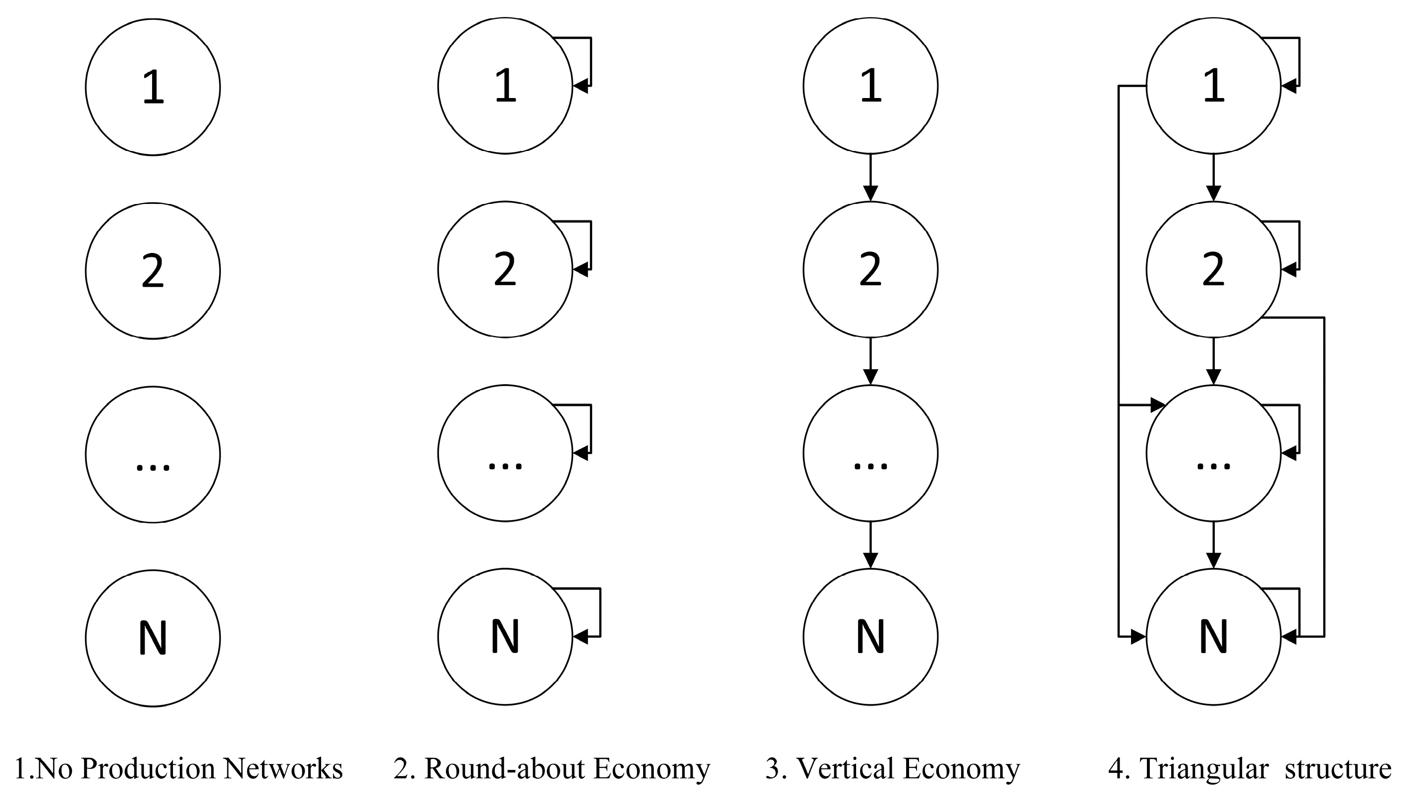
1. No Production Networks. In the case of no production network structure, the fact that A is a zero matrix leads to $A^{\left(j\right)}=0$. Consequently, the input-output covariance ${\mathrm{Cov}}_{A^{\left(j\right)}}\left(L_{\left(k\right)},L_{\left(l\right)}\right)$ is constant 0, leading to zero second-order effects. It can be concluded that the structure of the production network is a necessary condition for second-order effects under single-input factor conditions.

2. Round-about Economy. In the case where a sector utilizes intermediate goods produced by itself, the presence of the production network ensures that the second-order impact is non-zero. Substitute the technical coefficient matrix and the Leontief matrix into Equation (22) yields:

$${\displaystyle \frac{d\mathit{log}Y}{d\mathit{log}{z}_{l}d\mathit{log}{z}_k}}={\displaystyle \frac{d{d}_l}{d\mathit{log}{z}_k}}=\{\begin{array}{c}0, l\ne k,\\ {\displaystyle \frac{a_{kk}}{1-a_{kk}}}{d}_k\left({\theta }_k-1\right), l=k.\end{array}$$

On the one hand, productivity shocks in sector $k$ have no effect on the sales share of sector $l \left(l \ne k\right)$ since each sector operates as an independent entity. On the other hand, the productivity shock in sector $k$ influences its own sales share, and we define the network-related term $\left(a_{kk}/1-a_{kk}\right)$ as the second-order intra-sector feedback. In particular, the size of the second-order feedback effect within a sector is only $a_{kk}$ times the size of the first-order effect. Consequently, the second-order effect is smaller than the first-order effect, indicating that the impact diminishes with increasing order.

3. Vertical Economy. When there is a strict upstream-downstream relationship between sectors, their first-order effects are amplified through input-output relationships, with the magnitude remaining as $a_{ij}$. Considering the second-order effects, we substitute the technical coefficient matrix and the Leontief matrix into Equation (22) yields:

$${\displaystyle \frac{d\mathit{log}Y}{d\mathit{log}{z}_{l}d\mathit{log}{z}_k}}={\displaystyle \frac{d{d}_l}{d\mathit{log}{z}_k}}=\{\begin{array}{cc}0,\hfill & \hfill \mid l-k\mid >1, \mathit{or} l=k=1\\ (a_{k-2,k-1}{a}_{k-1,k}^2-a_{k-2,k-1}^2{a}_{k-1,k}^2)d_{k-2}({\theta }_{k-2}-1)+(a_{k-1,k}-a_{k-1,k}^2)d_{k-1}({\theta }_{k-1}-1),\hfill & \hfill l=k\ne 1 \mathit{or} N\\ (a_{k-1,k}{a}_{k,k+1}-a_{k-1,k}^2{a}_{k,k+1})d_k({\theta }_k-1),\hfill & \hfill l-k=1\\ (a_{l-1,l}{a}_{l,l+1}-a_{l-1,l}^2{a}_{l,l+1})d_l({\theta }_l-1),\hfill & \hfill k-l=1\\ (a_{N-1,N}-a_{N-1,N}^2)d_{N-1}({\theta }_{N-1}-1).\hfill & \hfill l=k=N\end{array}$$

For example, for the sales share $d_3$, it is affected by shocks from both $\mathrm{d}\log z_2$ and $\mathrm{d}\log z_3$, with the magnitudes of the shocks given by:

$${\displaystyle \frac{d{d}_3}{d\mathit{log}{z}_2}}=\left(a_{12}{a}_{23}-a_{12}^2{a}_{23}\right)d_2\left(1-{\theta }_2\right),$$

$${\displaystyle \frac{d{d}_3}{d\mathit{log}{z}_3}}=\left(a_{12}{a}_{23}^2-a_{12}^2{a}_{23}^2\right)d_1\left(1-{\theta }_1\right)+\left(a_{23}-a_{23}^2\right)d_2\left(1-{\theta }_2\right).$$

It can be concluded that, first, in the absence of a feedback structure, the response of sector $i$’s sales share $d_i$ to a shock is independent of its own sales share. Second, due to the vertical structure between sectors, where no sector acts as both an input provider and user for the same set of sectors, the sales share of sector $i$ is independent of the productivity shock in sector $\left(i-2\right)$ and further downstream sectors. For instance, the partial derivative of $d_3$ with respect to sector 1 shocks is equal to zero. Third, the response of $d_i$ to a shock does not depend on the sales share of sector $\left(i-3\right)$ and further downstream departments. For example, the partial derivatives of $d_4$ with respect to shocks in arbitrary sectors are independent of $d_1$. In summary, the response of sales share of sector $i$ to shocks is determined by three factors: the production network structure, the elasticity of substitution, and the sales share of some downstream sectors. After excluding the intra-sectoral feedback effect, we refer to the amplification of the production network as the second-order inter-sectoral production network effect.

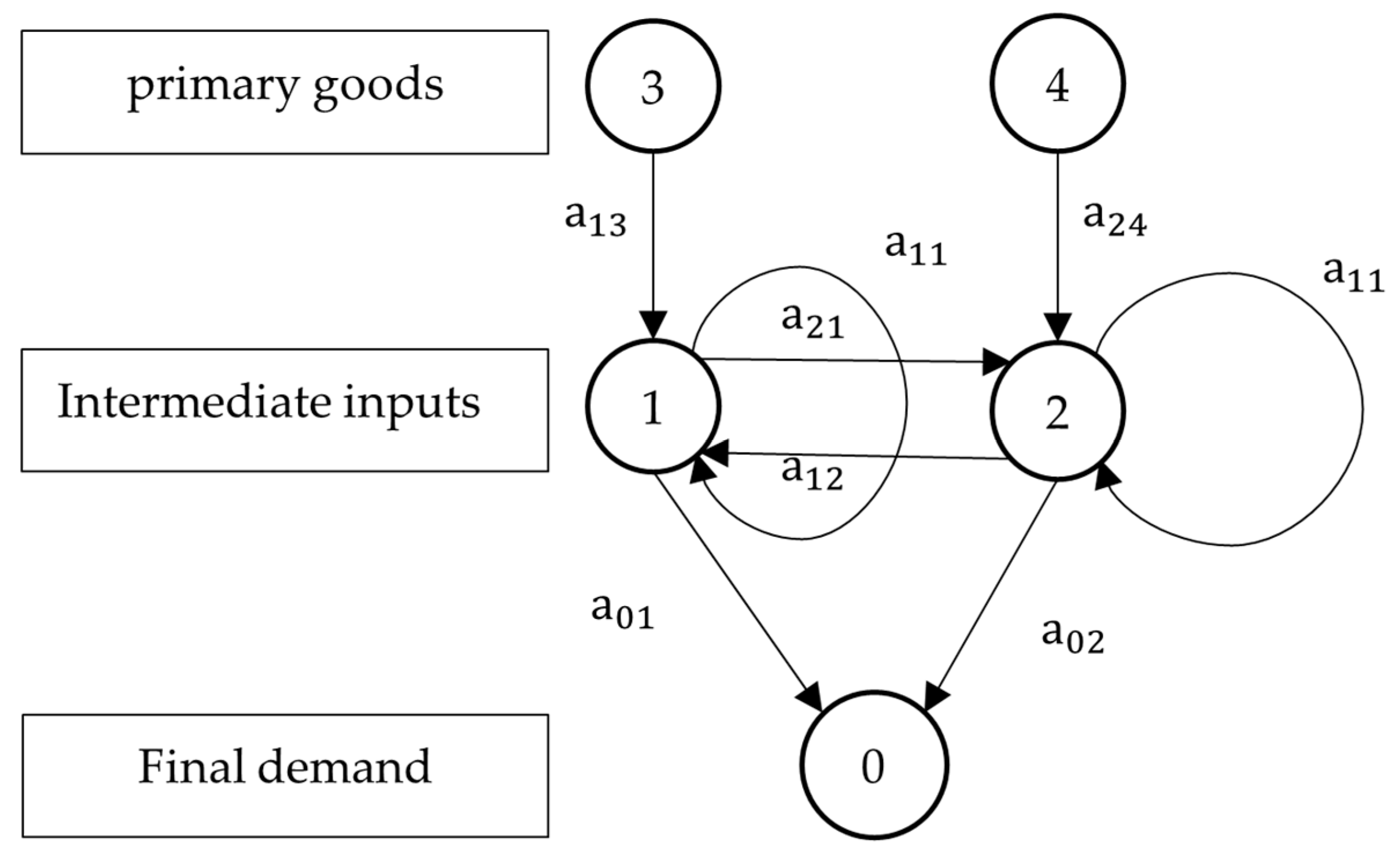
Next, we introduce the production network with a triangular structure into the second-order propagation formula for productivity shocks and analyze its propagation mechanism. The production network with a triangular structure not only contains the intra-sectoral feedback effect and inter-sectoral production network effect but also entails more complex input-output linkages between sectors. In addition, for simplification purposes, the final demand (sector 0 in Section 3.2) was not included in the previous model. However, the influence of the final demand is explored here.

First, consider a (4 × 4) triangular production network structure comprising two production sectors, a primary factor sector, and a final demand sector, where production sector 1 is positioned downstream and production sector 2 is located upstream. The technical coefficient matrix and the Leontief inverse matrix are given by:

$$A=\left(\begin{array}{cccc}0& c_1& c_2& 0\\ 0& a_{11}& a_{12}& f_1\\ 0& 0& a_{22}& f_2\\ 0& 0& 0& 0\end{array}\right),$$

$$L=\left(\begin{array}{cccc}1& {\displaystyle \frac{c_1}{1-a_{11}}}& {\displaystyle \frac{c_1{a}_{12}}{\left(1-a_{11}\right)\left(1-a_{22}\right)}}+{\displaystyle \frac{c_2}{1-a_{22}}}& {\displaystyle \frac{c_1{f}_2{a}_{12}}{\left(1-a_{11}\right)\left(1-a_{22}\right)}}+{\displaystyle \frac{c_1{f}_1}{1-a_{11}}}+{\displaystyle \frac{f_2{c}_2}{1-a_{22}}}\\ 0& {\displaystyle \frac{1}{1-a_{11}}}& {\displaystyle \frac{a_{12}}{\left(1-a_{11}\right)\left(1-a_{22}\right)}}& {\displaystyle \frac{f_2{a}_{12}}{\left(1-a_{11}\right)\left(1-a_{22}\right)}}+{\displaystyle \frac{f_1}{1-a_{11}}}\\ 0& 0& {\displaystyle \frac{1}{1-a_{22}}}& {\displaystyle \frac{f_2}{1-a_{22}}}\\ 0& 0& 0& 1\end{array}\right).$$

Thus, the second-order impact of a sectoral productivity shock is given by:

$${\displaystyle \frac{d{d}_1}{d\mathit{log}{z}_1}}=\left[{\displaystyle \frac{c_1}{{\left(1-a_{11}\right)}^2}}-{\displaystyle \frac{c_1^2}{{\left(1-a_{11}\right)}^2}}\right]d_0\left({\theta }_0-1\right)+{\displaystyle \frac{a_{11}}{1-a_{11}}}{d}_1\left({\theta }_1-1\right),$$

$${\displaystyle \frac{d{d}_1}{d\mathit{log}{z}_2}}={\displaystyle \frac{d{d}_2}{d\mathit{log}{z}_1}}={\alpha }_0{d}_0\left({\theta }_0-1\right)+{\alpha }_1{d}_1\left({\theta }_1-1\right),$$

$${\displaystyle \frac{d{d}_2}{d\mathit{log}{z}_2}}={\beta }_0{d}_0\left({\theta }_0-1\right)+{\beta }_1{d}_1\left({\theta }_1-1\right)+{\displaystyle \frac{a_{11}}{1-a_{11}}}{d}_2\left({\theta }_2-1\right),$$

where ${\alpha }_0$, ${\alpha }_1$, ${\beta }_0$, ${\beta }_1$ are parameters related to the structure of the production network, which can be expressed as a combination of intra-sectoral feedback effects and inter-sectoral production network effects. Unlike the previous inter-sectoral production network effect, the second-order effect of sector $i$ on $j$ may be amplified again by intra-sectoral feedback from sector $j$. Thus, the second-order effect of the inter-sectoral production network in this case is amplified due to intra-sectoral and inter-sectoral interactions. On the other hand, for the second-order effect of a productivity shock in sector $i$ on itself, the linear component on the right-hand side of the equation, associated with its own sales share, represents the purely intra-sectoral feedback effect. Meanwhile, the linear component associated with the sales shares of other sectors is a combination of both the inter-sectoral production network effect and the intra-sectoral feedback effect.

Based on the above formula, the following important insights can be drawn: First, the second-order effects of microeconomic shocks are symmetric, due to the symmetry inherent in the covariance structure of the production network. This finding aligns with the conclusions of Baqaee and Farhi [31]. Second, the effect of productivity shocks in sectors 1 and 2 on the sales share of sector 1 is positively proportional to $d_0$, $d_1$, the effect of productivity shocks in sector 1 on the sales share of sector 2 is proportional to $d_0$, $d_1$, and the effect of productivity shocks in sector 2 on the share of sales in sector 2 is proportional to $d_0$, $d_1$, $d_2$. As a result, the productivity shock affects the sales shares of all sectors both upstream and downstream, and the second-order effect on the macroeconomy is non-zero. In the absence of production networks, the second-order impact on the macroeconomy would remain zero. Therefore, production networks induce a second-order impact by affecting the sales shares of all sectors.

Written in a unified equation, the magnitude of the second-order impact can be expressed as:

$${\displaystyle \frac{d\mathit{log}Y}{d\mathit{log}{z}_{l}d\mathit{log}{z}_k}}={\displaystyle \frac{d{d}_l}{d\mathit{log}{z}_k}}={\displaystyle \sum }_{i=0}^{\mathit{min}\left(l,k\right)}{\gamma }_i{d}_i\left(1-{\theta }_i\right),$$

(23)

where ${\gamma }_i$ is a parameter related to the structure of the production network. Changes in sectoral sales shares are related to factor substitution between sectors. Since the products of sector i are only used as intermediate inputs in the downstream sectors, only these downstream sectors can substitute for them. As a result, the change in the sales share of sector $i$ is only related to the elasticity of substitution and sales share of its downstream sectors. Extending the above triangular production network structure to sector N, the following theorem can be obtained:

Theorem 4

(Second-order propagation of microeconomic shocks in the triangular production network structure). In the triangular production network structure, there are two important conclusions, which are as follows:

(1) 

The magnitude of the effect of a productivity shock in sector$i$on the sales share of sector$j$is always greater than 0. This magnitude depends on (i) the elasticity of substitution from sector 0 to sector$min\left(i,j\right)$and (ii) the sales share from sector 0 to sector$min\left(i,j\right)$. The effect of a productivity shock in sector$i$on the sales share in sector$j$is simultaneously propagated upstream and downstream.

(2) 

The magnitude of the second-order impact of a productivity shock in sector $i$ depends on (i) the elasticity of substitution of sector $i$ and its downstream sectors and (ii) the sales share of sector $i$ and its downstream sectors. Additionally, the second-order impact of a productivity shock in sector $i$ propagates both upstream and downstream.

Finally, we analyze the propagation mechanism of microeconomic shocks based on the above results. We first introduce the effect of productivity shocks on product prices under a single primary input:

$${\displaystyle \frac{d\mathit{log}{p}_i}{d\mathit{log}{z}_j}}=-L_{ij}.$$

(24)

Thus, the second-order effects of factor productivity shocks can be rewritten as:

$${\displaystyle \frac{d\mathit{log}Y}{d\mathit{log}{z}_{l}d\mathit{log}{z}_k}}={\displaystyle \frac{d{d}_l}{d\mathit{log}{z}_k}}={\displaystyle \sum }_j\left({\theta }_j-1\right)d_j{\mathit{Cov}}_{A^{\left(j\right)}}\left({\displaystyle \frac{d\mathit{log}p}{d\mathit{log}{z}_k}},L_{\left(l\right)}\right).$$

(25)

Thus, the first major effect of the productivity shock of sector $k$ is the price effect on each sector, which is measured by the $k$ column $L_{\left(k\right)}$ of the $\mathit{L}$ matrix. In a triangular production network, $L_{ik}=0$ if $i>k$. In this case, productivity shocks in sector $k$ only affect prices downstream. As a result, the price impact of a productivity shock is transmitted downstream. However, in the real economy, prices in the downstream sectors often exert an inverse forcing mechanism on the prices in the middle and upstream sectors. Characterizing such a forcing mechanism presents an important direction for future model development.

After the primary impact, the relative price changes induce each producer to substitute its factors, with the elasticity of substitution playing a crucial role in determining the extent of this adjustment. Assume that there are only two inputs $k$ and $l$. Their sales are $x_k{p}_k$ and $x_l{p}_l$, respectively, and the elasticity of substitution between the two inputs by the producer is $\theta$, then we have:

$$-{\displaystyle \frac{d\mathit{log}\left(x_k{p}_k/x_l{p}_l\right)}{d\mathit{log}\left(p_k/p_l\right)}}=\theta -1,$$

(26)

where the effect of elasticity of substitution on relative sales under relative price changes is summarized by $\theta -1$, which explains the presence of the term $\left({\theta }_j-1\right)$ in the second-order effect.

After the definition, we return to the derivation following the relative price change. Sector $j$ substitutes goods in sector l with other goods. When ${\theta }_j<1$, a rise in the relative price of sector l implies an increase in the relative input share, leading to higher Domar weights. The magnitude of this substitutability is measured by the input-output covariance ${\mathit{Cov}}_{A^{\left(j\right)}}\left(\mathrm{d}\log p/\mathrm{d}\log z_k,L_{\left(l\right)}\right)$. Among this, the probability $A^{\left(j\right)}$ of the covariance represents the interchangeable inputs of sector $j$, including inputs from sector $l$; $\mathrm{d}\log p/\mathrm{d}\log z_k$ denotes the size of price change in each sector following the productivity shock in sector k; $L_{\left(l\right)}$ denotes the total demand coefficient for sector $l$ in each sector. Ultimately, the effect of sector $k$’s productivity shock on sector $l$’s sales share is equal to the sum of impact from input substitution by all sectors to sector $l$. When the input-output covariance increases, the relative relationship between sector $l$ and the prices of the sectors becomes stronger, leading to a greater input substitution of sector $j$ for sector $l$.

Overall, the second major impact of the productivity shock in sector $k$ is a change in the share of sales in sector $l$ caused by a change in prices in each sector. The second-order impact of the productivity shock is transmitted upstream because sector $j$ substitutes for goods upstream. Combining the first and second impacts, the second-order impacts of sectoral productivity shocks are transmitted both upstream and downstream along the supply chain, so that the second-order impacts on all sectors are not zero.

In the special triangular production network case, the impact mechanism of sector $k$’s productivity shock on the factor income share of sector $l$ can be analyzed in detail. The first major effect influences the prices of the sector and its downstream sectors, and the second major effect arises from factor substitutions made by sector $j$. On the one hand, sector $j$ is downstream of sector $l$ because it relies on intermediate inputs from sector $l$, so that $k<l$. On the other hand, price shocks must propagate through inputs in sector $j$, and prices of the sector and its downstream sectors change, so sector $j$ is downstream of sector $k$, i.e., $j<k$. In all, $j<min\left(k,l\right)$, which is the same result as in Theorem 4. There are two conditions under which the sales share of sector $j$ contributes to the impact of the sector $k$’s shock on sector $l$: (1) sector $j$ uses intermediate inputs from sector $l$, and (2) the price of the intermediate inputs used by sector $j$ is affected by the price shock.

4.2.2. Propagation Mechanisms with Multiple Factors

In the previous section, we analyzed the second-order propagation mechanism of productivity shocks under a single primary input. However, in real-world scenarios, there are multiple factors. Next, we explore the propagation mechanism under multiple factors.

Theorem 5.

The second-order impact of productivity shocks with multiple factors is:

$$\begin{array}{ll}{\displaystyle \frac{d^2\mathit{log}Y}{d\mathit{log}{z}_{l}d\mathit{log}{z}_k}}& ={\displaystyle \frac{d{d}_l}{d\mathit{log}{z}_k}}={\displaystyle {\displaystyle \sum }_j}\left({\theta }_j-1\right)d_j{\mathit{Cov}}_{A^{\left(j\right)}}\left(L_{\left(k\right)},L_{\left(l\right)}\right)-{\displaystyle {\displaystyle \sum }_f}{\displaystyle \frac{d log{D}_f}{d log{z}_k}}{\displaystyle {\displaystyle \sum }_j}\left({\theta }_j-1\right)d_j{\mathit{Cov}}_{A^{\left(j\right)}}\left(L_{\left(f\right)},L_{\left(l\right)}\right)\\ & ={\displaystyle {\displaystyle \sum }_j}\left({\theta }_j-1\right)d_j{\mathit{Cov}}_{A^{\left(j\right)}}\left(L_{\left(k\right)}-{\displaystyle {\displaystyle \sum }_f}{\displaystyle \frac{d log{D}_f}{d log{z}_k}}{L}_{\left(f\right)},L_{\left(l\right)}\right)\end{array},$$

(27)

where the third equality is derived from the linear properties of the covariance operator. By replacing the sales share $d_l$ in the above formula with the factor income share $D_f$ , the impact of the productivity shock on the factor income share can be expressed as follows:

$${\displaystyle \frac{d log{D}_f}{d log{z}_k}}={\displaystyle {\displaystyle \sum }_j}\left({\theta }_j-1\right){\displaystyle \frac{d_j}{D_f}}{\mathit{Cov}}_{A^{\left(j\right)}}\left(L_{\left(k\right)},L_{\left(f\right)}\right)-{\displaystyle {\displaystyle \sum }_g}{\displaystyle \frac{d log{D}_g}{d log{z}_k}}{\displaystyle {\displaystyle \sum }_j}\left({\theta }_j-1\right){\displaystyle \frac{d_j}{D_f}}{\mathit{Cov}}_{A^{\left(j\right)}}\left(L_{\left(g\right)},L_{\left(f\right)}\right),$$

(28)

which can be rewritten in matrix form as:

$${\displaystyle \frac{d logD}{d log{z}_k}}=\gamma {\displaystyle \frac{d logD}{d log{z}_k}}+{\delta }_{\left(k\right)},$$

(29)

where the elements of $\gamma$ and ${\delta }_{\left(k\right)}$ are denoted by:

$${\gamma }_{fg}=-{\displaystyle \frac{1}{D_f}}{\displaystyle \sum }_j{d}_j\left({\theta }_j-1\right)Co{v}_{A^{\left(j\right)}}\left(L_{\left(g\right)},L_{\left(f\right)}\right),$$

(30)

$${\delta }_{fk}={\displaystyle \frac{1}{D_f}}{\displaystyle \sum }_j{d}_j\left({\theta }_j-1\right)Co{v}_{A^{\left(j\right)}}\left(L_{\left(k\right)},L_{\left(f\right)}\right).$$

(31)

It can be seen from the second equality of Equation (27) that the first term in the case of multiple factors is the same as that in the case of a single factor. Therefore, the propagation mechanism of this term is also transmitted both upstream and downstream, and the magnitude of the second-order influence is only related to the downstream factor income share. However, in the case of multiple primary inputs, the microeconomic productivity shock also affects the sales share through the factor reallocation effect.

Equations (28)–(31) analyze in detail the impact of productivity shocks on factor income shares. The impact comes from two sources. First, the factor income share of factor $f$ is directly affected by the productivity shock of sector $k$ with the magnitude determined ${\delta }_{fk}$. When the relative price of factors is not considered, the productivity shock of sector $k$ can be described by Equation (22). Therefore, the direct effect ${\delta }_{fk}$ without factor substitution can be obtained by just replacing the corresponding sector index $l$ with $k$. The change of factor income share will cause the change of factor price. To analyze this mechanism, we introduce the relationship between factor price $w_f$ and factor income proportion $D_f$ as:

$${\displaystyle \frac{d log w_f}{d log D_f}}=L_{if}.$$

(32)

A change in factor prices, like a change in product prices, will further induce changes in the share of all sectors. Particularly, it will cause changes in factor income shares. Replace $L_{\left(k\right)}$ in Formula (22) with $L_{\left(f\right)}$ to represent the change in factor income shares caused by factor price changes. Changes in the factor income share in turn cause further changes in relative factor prices, and the process repeats itself. Finally, the change of factor income shares is expressed as a multidimensional fixed-point equation.

After analyzing the change in factor income shares, we now return to the change in sales shares or Domar weights in the production sectors. The change also consists of two parts (shown in Figure 3). First, sectoral productivity shocks cause price changes in their own and in downstream sectors, inducing input substitution in more downstream sectors, which results in changes in the sales share in all sectors. Second, the productivity shock causes price changes in both the sector itself and its downstream sectors, leading to changes in factor income shares. The change in factor prices, in turn, causes changes in the prices of the product sectors that utilize the factor, which leads to input substitution in the downstream sectors, ultimately resulting in changes in the sales shares of all sectors. Changes in sectoral sales shares result from both changes in product prices and changes in factor prices. In addition, there is a feedback mechanism between changes in factor prices and changes in factor income shares. Since primary factors can be considered the most upstream sector, productivity shocks in any sector can influence factor prices.

To further analyze the pattern of shock propagation, attention should be given to the last equality of Equation (27), where the change in prices due to microeconomic shocks is:

$${\displaystyle \frac{d log p_i}{d log A_k}}=L_{ik}-{\displaystyle \sum }_f{\displaystyle \frac{d log D_f}{d log z_k}}{L}_{if}.$$

(33)

Thus, the second-order effects of productivity shocks under multiple primary inputs can still be categorized into a twofold impact. The first impact consists of two paths: one directly through the production network, and the other by affecting factor income shares, which in turn impacts factor prices and is transmitted to the sectors that use these factors. In terms of direction, both product and factor prices are transmitted downstream, establishing a downstream propagation path. The second impact of the productivity shock mirrors that in the case of a single primary input, representing an upstream propagation path. Therefore, sectoral productivity shocks are transmitted both upstream and downstream simultaneously, ultimately leading to changes in the sales shares of all sectors.

To explore how the factor reallocation effect works, we begin with a simple case of a factor self-input structure. Assuming that there is a final demand sector, a self-input sector, and two primary factors in the economy, the corresponding direct requirements matrix and Leontief inverse Matrix are:

$$A=\left(\begin{array}{cccc}0& c_1& 0& 0\\ 0& a_{11}& f_{11}& f_{12}\\ 0& 0& 0& 0\\ 0& 0& 0& 0\end{array}\right), L=\left(\begin{array}{cccc}1& {\displaystyle \frac{c_1}{1-a_{11}}}& {\displaystyle \frac{f_1{c}_1}{1-a_{11}}}& {\displaystyle \frac{f_2{c}_1}{1-a_{11}}}\\ 0& {\displaystyle \frac{1}{1-a_{11}}}& {\displaystyle \frac{f_1}{1-a_{11}}}& {\displaystyle \frac{f_2}{1-a_{11}}}\\ 0& 0& 1& 0\\ 0& 0& 0& 1\end{array}\right),$$

where $f_{ij}$ denotes the primary factor input coefficient, which refers to the value of primary inputs in the total output of each sector. Thus, the second-order effect is given by:

$${\displaystyle \frac{d^2\mathit{log}Y}{d log z_{1}d log z_1}}={\displaystyle \frac{d{d}_1}{d log z_1}}=\xi -{\displaystyle \frac{D_2{f}_1^2+D_1{f}_2^2}{D_1{D}_2+D_2{f}_1^2\xi +D_1{f}_2^2\xi }}{\xi }^2,$$

where ξ is the second-order effect under a single factor, which can be expressed as:

$$\xi ={\displaystyle \frac{a_{11}}{{\left(1-a_{11}\right)}^2}}{d}_1\left({\theta }_1-1\right).$$

Several interesting findings can be derived from the above equations. First, when there are two factors, the impact of the shock is related to the factor income shares $D_1$, $D_2$ and the primary factor input coefficient $f_1$, $f_2$ for both factors. Second, when there is only one production sector, the final demand expenditure share is 1 as there is only one final good. The coefficient on the term containing ${\theta }_0$, $d_0$ is zero because the final demand sector is no longer substituting inputs in this case. Third, multiple primary inputs reduce the magnitude of the second-order effect of productivity shocks through factor income shares, so the factor reallocation effect acts as a negative feedback process.

We extend the above results to a generalized triangular production network structure. First, in terms of relevance, the second-order effects of sectoral productivity shocks are correlated with both the factor income shares and primary factor input coefficients of each factor due to changes in factor income shares and relative factor prices. Moreover, changes in relative factor prices provide an additional mechanism for sectoral substitution, which can also be transmitted upstream. As a result, the second-order effects, in general, are correlated with the sales shares (Domar weights) of each production sector. Second, in terms of magnitude, the impact through factor income shares, and hence relative factor prices, is negative, which attenuates the second-order impact through downstream substitution alone in the case of a single factor. Third, in terms of calculation, when the number of production sectors exceeds 2, the inverse matrix becomes highly complicated, resulting in the absence of a corresponding analytical or closed-form solution. Therefore, numerical solutions must be used in practice to derive results.

5. Quantitative Analysis

We quantitatively analyze the models developed in the previous sections. Given that the triangular input-output structure significantly simplifies the propagation formula, thereby facilitating the analysis of the propagation mechanism, a fundamental question arises: does the production network in the real economy exhibit a triangular structure? Encouragingly, after processing China’s 2018 input-output tables, we find that the answer is affirmative. This finding suggests that certain sectors predominantly serve as suppliers, while others function primarily as users. From a theoretical perspective, the asymmetry inherent in the production network can significantly influence the propagation of productivity shocks. Building on the parameters of the triangular production network structure, this section further simulates both the first-order and second-order propagation of shocks. On the one hand, it examines the structural characteristics of the production network and the associated propagation mechanisms. On the other hand, it identifies the key factors involved in the propagation of productivity shocks, providing a practical foundation for policymaking.

5.1. Triangle Production Network Structure in China

First, we adjust China’s 2018 input-output table using the matrix triangulation method proposed by Simpson and Tsukui [23]. The triangular production network structure is characterized by the concentration of matrix elements in one triangle, which means that sector $i$ uses the products of sector $\left(i+1\right)$, but sector $\left(i+1\right)$ does not use the products of sector $i$. However, in the production network of a real economy, even if the elements are concentrated in one triangle, the elements of the other triangle cannot all be 0. Therefore, an approximate triangulation is adopted here. Simply put, a row-column comparison approach is taken, where larger elements are gradually moved to one corner of the matrix and smaller elements are gradually moved to the other opposite corner of the matrix. After that, there are two possible scenarios. In the first case, the diagonal of the set of small elements is not zero and the proportion of non-zero elements is large. Therefore, we call the previous matrix a non-triangular matrix. In the second case, the diagonal of the set of small elements is almost zero so that the processed matrix can be transformed into a quasi-triangular matrix. Thus, we call the previous matrix a triangular matrix.

Figure 4 presents the triangular production network matrix for China’s 42 × 42 sectors in 2018. This matrix is defined as the transpose of the classical technical coefficient matrix, consistent with the definition used in the previous model. It is evident that the elements of the matrix are predominantly concentrated in the upper-right corner. Specifically, sector 1 is characterized by having the largest number of sectors as users and the fewest as inputs, making it the most downstream sector. In contrast, sector 42 has the largest number of sectors as inputs and the fewest as users, rendering it the most upstream sector. To verify this structure, we calculated the proportion of the sum of the elements in the upper-right corner and the sum of the elements in the lower-left corner, respectively. The sum of the elements in the upper-right corner accounts for 65.93%, and when combined with the proportion of the diagonal elements, the total reaches 87.70%. These findings suggest that China’s 2018 technical coefficient matrix is triangulable. This result is consistent with Liu (2019), who derived similar findings from China’s 2007 input-output matrix, further underscoring the stability of the triangular structure of China’s production network.

To better analyze the impact of the triangular production network structure, we introduce the concept of sector essentiality. Sector 1 is said to be more fundamental than sector 2 if sector 2 uses the products produced by sector 1 while sector 1 does not use the products produced by sector 2. Compared to the concept of “upstream”, “sector essentiality” better reflects the necessity of a sector within the industrial chain. When analyzing the propagation of microeconomic shocks, we use “more essential” and “more upstream” interchangeably. After triangulating the input-output matrix, we obtain the ranking of sector essentiality (as shown in

Table 3. Top 10 sectors in terms of sectoral essentiality and their numbers.

Sector	Ranking of Sector Essentiality
Finance	42
Real estate	41
Transportation, storage, and postal services	40
Leasing and business services	39
Wholesale and retail	38
Coal mining and processing	37
Electricity and heat production and supply	36
Chemical products	35
Agricultural, forestry, animal husbandry, fishery products and services	34
Food and tobacco	33

Note. The higher the ranking of sector essentiality, the more fundamental the sector.

). A higher ranking of sector essentiality indicates a more essential sector. Accordingly, the top 10 sectors by sector essentiality are finance, real estate, transportation, storage and postal services, leasing and business services, wholesale and retail, coal mining and processing, electricity and heat production and supply, chemical products, agricultural, forestry, animal husbandry, and fishery products and services, as well as food and tobacco. These essential sectors exhibit distinct characteristics: agricultural sectors include agricultural, forestry, animal husbandry, and fishery products and services, as well as food and tobacco. Industrial raw materials, fuels, and auxiliary materials encompass coal mining and processing, electricity and heat production and supply, and chemical products. Meanwhile, productive service sectors include finance, transportation, storage and postal services, leasing and business services, and wholesale and retail. The results here are similar to Lin [39]’s findings on the essentiality ranking of sectors in China. In the input-output matrix, inputs of capital goods are as important as inputs of intermediate goods across sectors. However, China does not officially publish an investment matrix, making it impossible to obtain data on capital goods inputs. Since this study primarily focuses on the propagation mechanisms within triangular production networks rather than determining the relative importance of individual sectors, the absence of an investment matrix does not affect the subsequent simulation of sectoral productivity shocks.

5.2. First-Order Effects

We first simulate the first-order propagation of productivity shocks. Assuming a one-unit shock to each sector, the magnitude of the first-order impact is determined solely by the sector’s Domar weight. The relationship between Domar weights and the ranking of sector essentiality is illustrated in Figure 5. Here, there are several key findings: First, in terms of magnitude, the maximum Domar weight is 0.290 (construction), while the minimum is 0.002 (repair services for metal products, machinery, and equipment). The ratio between the two sectors’ Domar weights is 146, indicating significant variation in the impact of productivity shocks across sectors on the overall economy. Second, when regarding trends, Domar weights and the ranking of sector essentiality are generally positively correlated. In other words, the more essential a sector (higher in the ranking), the larger its Domar weight. This can be explained using the model: in a triangular production network, shocks propagate downstream along the supply chain, determined only by the final demand expenditure share of downstream sectors. A more essential (more upstream) sector propagates its shocks to a greater number of sectors, leading to a more complex composition of its Domar weight. However, this relationship is not strictly linear. When the total demand coefficients between two intermediate sectors are sufficiently large, it may lead to the first-order impact on downstream sectors being greater than the first-order impact on upstream sectors.

The Domar weight can be further decomposed into two components: one is the final demand effect, and the other is the production network effect, which consists of both intra-sectoral feedback effects and inter-sectoral production network effects. Figure 6 shows the relationship between the final demand effect of each sector in China and its sector essentiality ranking. From the figure, it can be observed that, except for sector 9 (construction), the final demand effects of the sectors fluctuate around the mean value of 0.024. There is no obvious relationship between the final demand effect and sector essentiality, suggesting that the final demand effect cannot be used to explain the relationship between sector essentiality and Domar weights. Furthermore, the final demand effect of sector 9 is significantly larger than that of other sectors, which is the main reason for its Domar weight being much higher than those of other sectors.

Next, we focus on describing the total production network effects represented by the Leontief inverse matrix $L$. Figure 7 illustrates the results of these production network effects. In the matrix, the columns represent the sectors experiencing the shock, while the rows represent the sectors receiving the shock. If a matrix element is non-zero (colored in blue), it indicates that the shock from the sector represented by the column can propagate to the sector represented by the row. The deeper the color, the stronger the propagation intensity. From the figure, it is evident that the non-zero matrix elements are concentrated in the upper-right portion of the matrix, while elements in the lower-left portion are mostly zero. This confirms the previous conclusion: the shocks from upstream sectors (with higher sector numbers) primarily propagate to downstream sectors (with lower sector numbers).

To further discuss the results derived from the Leontief inverse matrix, we examine the impact of changes in the final demand effect on the economy. We select a sector with an intermediate ranking in sector essentiality (sector 21) and increase its final demand expenditure share by 0.1, while leaving other sectors unchanged. The resulting changes in Domar weights are shown in Figure 8. The figure shows that as the final demand expenditure share of sector 21 increases, the impact of productivity shocks on its upstream sectors changes significantly, while the impact on its downstream sectors changes relatively little. Since the first-order effects of productivity shocks propagate downstream, the impact of productivity shocks in upstream sectors is related to the final demand share of downstream sectors, while the impact of productivity shocks in downstream sectors is unrelated. Therefore, in a triangular production network structure, a change in the final demand effect of one sector will only affect the magnitude of productivity shocks to its upstream sectors.

Finally, Domar weights are determined by both the final demand effect and the production network effect. The latter exposes significant differences between upstream and downstream, and thus it explains the positive correlation between Domar weights and sector essentiality. This positive correlation suggests that the first-order effects of sectoral productivity shocks tend to be amplified as their fundamentals increase, and this amplification becomes more pronounced as the production network matrix tends to be more triangulated. Thus, sector essentiality is important in explaining economic development and volatility. Industrial policy should prioritize supporting fundamental sectors like finance, construction, and transportation. These sectors are vital for stable economic growth. Encouraging technological innovation can strengthen their resilience, helping to buffer the economy against negative productivity shocks.

5.3. Second-Order Effects

We consider the second-order effects due to sectoral unit productivity shocks. First, we define and explain the parameters involved in the simulation process. Unlike the first-order impact, the magnitude of the second-order impact depends on the sector’s Domar weight, elasticity of substitution, and input-output relationship. Unlike first-order effects, the magnitude of second-order effects depends on several factors: the Domar weight $d$, the technical coefficient matrix $A$, the Leontief inverse matrix $L$, the factor income share $D$, the elasticity of substitution $\theta$, and the magnitude of the shock $\mathrm{dlog}\left(z\right)$. We simulate the impact of a unit productivity shock, thus setting $\mathrm{dlog}\left(z\right)=1$. Based on the industry linkages in the input-output matrix, the Domar weight, the factor income share, and the two coefficient matrices can be calculated separately. Concerning the elasticity of intermediate goods, this study follows the parameterization approach employed in previous research, defines a reasonable range for the parameters, and selects values within this range that are most appropriate for the model under consideration. Atalay [40] estimates the substitution elasticity between inputs to range from 0.4 to 0.8. In line with the parameter settings adopted by Baqaee and Farhi [8], we specify the elasticity of substitution between value-added and intermediate inputs as 0.5 and the elasticity of substitution in consumption ${\theta }_0$ as 0.9. When $\theta >1$, there is a strong substitutability between inputs, meaning that an increase in the relative factor price of an input will lead to a decrease in its share. When $\theta =1$, the CES function degenerates into a Cobb–Douglas production function, implying a unitary elasticity of substitution between inputs. Conversely, when $\theta <1$, the substitutability between inputs is weak (indicating complementarity), and an increase in the relative factor price of an input will result in an increase in its share. Thus, the above setting implies that there is a complementary relationship both between inputs and between preferences. Additionally, we will also select two scenarios for comparison: $\theta =0$, representing the Leontief case, and $\theta =2$, representing the factor substitution case. We do not set $\theta =1$, as in this case, the second-order effects of productivity shocks are zero (because there is no change in input shares, the second-order effect under the Cobb–Douglas function is zero).

First, we present the second-order propagation when the elasticity of substitution between inputs is 0.5 (Figure 9). As shown in the figure, first, although most second-order shocks are numerically small, they are not zero. This verifies the conclusion that the second-order effects of productivity shock propagate to both the upstream and downstream along the industrial chain and that the second-order effects under the general production network are not zero. Second, the matrix exhibits a symmetric distribution, which implies that the impact of a shock in sector $j$ on the sales share of sector $i$ is the same as the impact of a shock in sector $i$ on the sales share of sector $j$. Fundamentally, this stems from the symmetry in the form of input-output covariances, which coincides with the related findings of Baqaee and Farhi [31]. Third, the second-order effect along the diagonal is negative, as a substitution elasticity of less than 1 results in a decline in the relative price of the industry itself, which in turn leads to a reduction in its relative sales share. Therefore, under conditions of input complementarity, the second-order effects primarily serve to attenuate the first-order effects, thereby alleviating the impact of negative shocks.

Next, we set the elasticity of substitution to zero to examine the propagation mechanism of productivity shocks under the case of perfect complements. Figure 10 illustrates the matrix distribution of the magnitude of the impact of second-order shocks when the elasticity of substitution $\theta =0$. The diagonal elements tend to be negative, while the off-diagonal elements tend to be positive. When the elasticity of substitution is less than one, a decrease in the relative price of the sector itself leads to a decrease in its relative sales share and a subsequent increase in the relative sales share of other sectors. Compared to the case with $\theta =0.5$, the diagonal elements are smaller. This can be explained by the formula with multiple factors, which suggests that when the elasticity of substitution is less than 1, a smaller elasticity results in larger second-order effects of productivity shocks on departments. This result aligns with the findings of Boehm et al. [32], whose analysis demonstrates that product complementarity enhances the propagation of shocks across firms. By adjusting the elasticity of substitution, second-order propagation exhibits similar characteristics when the elasticity of substitution is less than 1.

Subsequently, we investigate the scenario with a high elasticity of factor substitution. Figure 11 illustrates the second-order effects of productivity shocks when $\theta =2$. In comparison to the case where $\theta =0.5$, the second-order effects of the shock are predominantly positive. A positive productivity shock leads to a reduction in sectoral prices. When the elasticity of substitution between factors exceeds 1, this price reduction within the sector enhances its relative sales share while diminishing the relative sales share of other sectors. Furthermore, the positive second-order effect implies that despite the reduction in relative sales share, the absolute sales share of other sectors increases. According to the formula with multiple factors, when the elasticity of substitution is greater than 1, the larger the elasticity and the greater the second-order impact of sectoral productivity shocks. By altering the elasticity of substitution, second-order propagation exhibits similar characteristics when the elasticity of substitution exceeds 1.

Furthermore, we analyze the two mechanisms that underpin the observed second-order effects. In the first mechanism, the shock induces changes in the price of the downstream product through price effects, which directly leads to input substitution by users. In mechanism 2, changes in factor income shares and relative factor prices lead to price adjustments of products, thereby indirectly prompting input substitution by users. In addition, mechanism 1 is the only propagation mechanism of productivity shocks under a single factor scenario.

Taking the elasticity of substitution $\theta =0.5$ as an example, Figure 12 and Figure 13 illustrate the magnitude of the second-order impacts of productivity shocks, corresponding to the two mechanisms described above. First, at $\theta =0.5$, the magnitudes of the impacts resulting from the two mechanisms differ substantially, with the direct effect (Mechanism 1) being significantly larger than the indirect effect (Mechanism 2). This conclusion is consistent with Acemoglu [16], who argues that the upstream effects of productivity shocks are substantially smaller than the downstream effects. Mechanism 2, in this study, corresponds precisely to the upstream effects. Second, the impacts generated by mechanism I are distributed on the diagonal of the matrix, while the impacts generated by mechanism II are distributed on both the diagonal and the non-diagonal elements. Thus, second-order propagation through mechanism I acts primarily on intra-sectoral feedback, while second-order propagation through mechanism II also acts on production networks. This may be due to two reasons: on the one hand, there is upstream and downstream attenuation in the price propagation mechanism of mechanism I; on the other hand, mechanism II may be amplified through the interaction between value added shares and relative factor prices.

Finally, by modifying the elasticity of substitution in a specific sector, we can further examine how the second-order propagation of productivity shocks in other sectors is influenced by this sector, thereby identifying the direction of shock propagation. Specifically, we increase the elasticity of factor substitution in sector 21 (the middle sector) from 0.5 to 0.9. The differences in the second-order effects between the treatment and control groups are then compared, with the elasticity of substitution for all other sectors remaining fixed at 0.5. As shown in Figure 14, the elasticity of factor substitution of sector 21 mainly affects the diagonal elements after sector 21 in the matrix. This confirms theorem 4: Second-order effects in a triangular production network structure depend only on (1) the elasticity of factor substitution from sector 0 to sector $\min \left(i,j\right)$ and (2) the share of sales from sector 0 to sector $\min \left(i,j\right)$. In summary, the price effect propagates downward, while the second-order transmission related to the elasticity of substitution propagates upward.

6. Conclusions and Discussion

This paper introduces a general equilibrium model with a production network to explain the propagation mechanism of microeconomic productivity shocks. Within the framework of production network theory, this paper innovatively incorporates a triangular production network structure and provides a detailed analysis of the upstream and downstream propagation mechanisms of microeconomic productivity shocks. These mechanisms are further validated and discussed through quantitative analysis. The main conclusions of the paper are as follows:

First, the first-order effects of microeconomic productivity shocks propagate downstream along the industrial chain, while the second-order effects of microeconomic productivity shocks propagate simultaneously upstream and downstream along the industrial chain.

Second, the first-order propagation mechanism of microeconomic productivity shocks involves changes in the prices of the affected sector and its downstream sectors, induced by the productivity shock. The second-order propagation mechanism occurs through two channels: one involves changes in the prices of the sector itself and its downstream sectors, leading to input substitution by further downstream sectors; the other occurs through the reallocation of factors, which alters relative factor prices and subsequently affects the prices faced by factor users, prompting further input substitution by downstream sectors. By altering the structure of the production network, these mechanisms can either be disrupted or reinforced, thereby smoothing macroeconomic fluctuations or enhancing the impact of technological progress.

Third, the production network contributes to both the first- and second-order effects of microeconomic productivity shocks. The impact of different shocks and production network structures can be attributed to three types of effects: final demand effects, intra-sectoral feedback effects, and inter-sectoral production network effects, the latter two of which are effects brought about by the production network. The structure of the production network plays a non-negligible role in the scope and magnitude of productivity shocks. By introducing a triangular production network structure, this paper finds that the magnitude of the first-order effect of a sector’s productivity shock depends solely on the final demand share of the downstream sectors and the direct input coefficients of the downstream sectors for the affected sector. Under single-factor conditions, the magnitude of the second-order effect of a sector’s productivity shock depends on the factor substitution elasticity of this sector and its downstream sectors, as well as the final demand share of this sector and its downstream sectors.

Fourth, actual economic data indicate that the production network structure matrix in China is triangulable. This suggests that the input-output linkages between certain sectors are unidirectional rather than bidirectional. Therefore, the analytical conclusions drawn from the triangular production network are also applicable to the analysis of the propagation of microeconomic shocks in China, providing valuable insights for formulating rational and accurate economic policies to address technological and external shocks.

Based on the above conclusions, this paper proposes the following policy recommendations. First, we emphasize the crucial role of production networks in the policy-making process, as they not only profoundly influence the propagation of microeconomic shocks but also serve as channels through which various policies affect the real economy. Second, given the strong amplifying effects of production networks in upstream industries, it is essential to provide substantial support for three kinds of fundamental sectors: agriculture, energy, and productive services such as finance and real estate. This will both mitigate the impact of productivity shocks on economic fluctuations and magnify the overall effects of technological progress. Finally, simulations of the real-world economy will aid in identifying the microeconomic origins of macroeconomic fluctuations, facilitating the accurate assessment of the impacts of microeconomic shocks, and enabling the precise formulation and implementation of monetary, fiscal, and industrial policies.

The analysis in this paper still possesses some limitations, which could serve as potential directions for future research. First, this paper focuses on productivity shocks and only examines the supply side. Existing literature has explored the demand side, for example, Acemoglu [16] argues that demand shocks (such as changes in imports or government spending) propagate upstream, meaning that the impact on upstream sectors is greater than on downstream sectors directly affected by the shock. Baqaee and Farhi [31] suggest that demand shocks can also be modeled as supply shocks. However, further research is needed to explore the magnitude, propagation direction, and mechanisms of demand shocks.

Second, the numerical simulation results presented in this paper primarily focus on the direction and magnitude of shock propagation, without estimating the actual impact of microeconomic shocks. On the one hand, the accuracy of the estimates is heavily dependent on the precise calibration of key parameters, such as sectoral productivity and factor substitution elasticity. A crucial task for future research will be to improve the model by incorporating more accurate calibrations. On the other hand, to fully leverage the potential of triangular production networks, future studies could examine specific exogenous shocks, thereby offering more targeted policy insights for real-world applications.

Third, the analysis in this paper relies on certain assumptions, particularly the efficient market hypothesis and the exogenous network hypothesis. First, the economy is characterized by various frictions and distortions, such as financial frictions and matching frictions. These frictions or distortions can lead to factor misallocation within a production network economy, resulting in a decline in overall Total Factor Productivity (TFP) and economic efficiency. Given that a significant portion of the impact of microeconomic shocks arises from factor reallocation, these frictions or distortions can influence both the magnitude and direction of microeconomic shocks. This misallocation provides a basis for formulating industrial policies within production networks [26]. Furthermore, endogenous production networks represent a significant topic within the current literature on production networks. When considering endogenous production networks, the structure or density of the network may evolve in response to microeconomic shocks, leading to uncertain effects on the magnitude and direction of shocks. One possible approach is to examine a specific type of microeconomic shock, such as automation within a particular sector, and examine its specific impact on the production network. Exploring the role of endogenous production networks through the lens of triangular production networks is a viable avenue for future research.

References

1. Carvalho, V.M.; Tahbaz-Salehi, A. Production Networks: A Primer. Annu. Rev. Econ. 2019, 11, 635–663. [Google Scholar] [CrossRef]
2. Leontief, W. The Structure of American Economy, 1919–1929: An Empirical Application of Equilibrium Analysis; Harvard University Press: Cambridge, MA, USA, 1941. [Google Scholar]
3. Lucas, R.E. Understanding Business Cycles. Carnegie-Rochester Conf. Ser. Public Policy 1977, 5, 7–29. [Google Scholar] [CrossRef]
4. Hulten, C.R. Growth Accounting with Intermediate Inputs. Rev. Econ. Stud. 1978, 45, 511–518. [Google Scholar] [CrossRef]
5. Gabaix, X. The Granular Origins of Aggregate Fluctuations. Econometrica 2011, 79, 733–772. [Google Scholar]
6. Jones, C.I. Misallocation, Economic Growth, and Input-Output Economics; National Bureau of Economic Research: Cambridge, MA, USA, 2011. [Google Scholar]
7. Acemoglu, D.; Carvalho, V.M.; Ozdaglar, A.; Tahbaz-Salehi, A. The Network Origins of Aggregate Fluctuations. Econometrica 2012, 80, 1977–2016. [Google Scholar] [CrossRef]
8. Baqaee, D.R.; Farhi, E. The Macroeconomic Impact of Microeconomic Shocks: Beyond Hulten’s Theorem. Econometrica 2019, 87, 1155–1203. [Google Scholar] [CrossRef]
9. Demir, B.; Fieler, A.C.; Xu, D.Y.; Yang, K.K. O-Ring Production Networks. J. Polit. Econ. 2024, 132, 200–247. [Google Scholar] [CrossRef]
10. Huang, H.; Manova, K.; Perello, O.; Pisch, F. Firm Heterogeneity and Imperfect Competition in Global Production Networks; CEPR Discussion Papers; CEPR: Paris, France; London, UK, 2024; Available online: https://cepr.org/publications/dp19408 (accessed on 21 January 2025).
11. Arkolakis, C.; Huneeus, F.; Miyauchi, Y. Spatial Production Networks; National Bureau of Economic Research: Cambridge, MA, USA, 2023. [Google Scholar]
12. Chen, S. International Production Networks and the Propagation of Financial Shocks. J. Int. Econ. 2024, 153, 104039. [Google Scholar] [CrossRef]
13. Luo, S. Propagation of Financial Shocks in an Input-Output Economy with Trade and Financial Linkages of Firms. Rev. Econ. Dyn. 2020, 36, 246–269. [Google Scholar] [CrossRef]
14. Acemoglu, D.; Ozdaglar, A.; Tahbaz-Salehi, A. Networks, Shocks, and Systemic Risk; National Bureau of Economic Research: Cambridge, MA, USA, 2015. [Google Scholar]
15. Carvalho, V.M.; Nirei, M.; Saito, Y.U.; Tahbaz-Salehi, A. Supply Chain Disruptions: Evidence from the Great East Japan Earthquake. Q. J. Econ. 2021, 136, 1255–1321. [Google Scholar] [CrossRef]
16. Acemoglu, D.; Akcigit, U.; Kerr, W. Networks and the Macroeconomy: An Empirical Exploration. NBER Macroecon. Annu. 2016, 30, 273–335. [Google Scholar] [CrossRef]
17. Kopytov, A.; Mishra, B.; Nimark, K.; Taschereau-Dumouchel, M. Endogenous Production Networks under Supply Chain Uncertainty. Econometrica 2024, 92, 1621–1659. [Google Scholar] [CrossRef]
18. Barrot, J.-N.; Sauvagnat, J. Input Specificity and the Propagation of Idiosyncratic Shocks in Production Networks. Q. J. Econ. 2016, 131, 1543–1592. [Google Scholar] [CrossRef]
19. Horvath, M. Cyclicality and Sectoral Linkages: Aggregate Fluctuations from Independent Sectoral Shocks. Rev. Econ. Dyn. 1998, 1, 781–808. [Google Scholar] [CrossRef]
20. Horvath, M. Sectoral Shocks and Aggregate Fluctuations. J. Monet. Econ. 2000, 45, 69–106. [Google Scholar] [CrossRef]
21. Dupor, B. Aggregation and Irrelevance in Multi-Sector Models. J. Monet. Econ. 1999, 43, 391–409. [Google Scholar] [CrossRef]
22. Chenery, H.B.; Watanabe, T. International Comparisons of the Structure of Production. Econom. J. Econom. Soc. 1958, 26, 487–521. [Google Scholar] [CrossRef]
23. Simpson, D.; Tsukui, J. The Fundamental Structure of Input-Output Tables, an International Comparison. Rev. Econ. Stat. 1965, 47, 434–446. [Google Scholar] [CrossRef]
24. Fukui, Y. A More Powerful Method for Triangularizing Input-Output Matrices and the Similarity of Production Structures. Econom. J. Econom. Soc. 1986, 54, 1425–1433. [Google Scholar] [CrossRef]
25. Kondo, Y. Triangulation of Input–Output Tables Based on Mixed Integer Programs for Inter-Temporal and Inter-Regional Comparison of Production Structures. J. Econ. Struct. 2014, 3, 2. [Google Scholar] [CrossRef]
26. Liu, E. Industrial Policies in Production Networks. Q. J. Econ. 2019, 134, 1883–1948. [Google Scholar] [CrossRef]
27. Korte, B.; Oberhofer, W. Triangularizing Input-Output Matrices and the Structure of Production. Eur. Econ. Rev. 1971, 2, 493–522. [Google Scholar] [CrossRef]
28. Baqaee, D.R.; Farhi, E. Productivity and Misallocation in General Equilibrium. Q. J. Econ. 2020, 135, 105–163. [Google Scholar] [CrossRef]
29. Acemoglu, D.; Azar, P.D. Endogenous Production Networks. Econometrica 2020, 88, 33–82. [Google Scholar] [CrossRef]
30. Long Jr, J.B.; Plosser, C.I. Real Business Cycles. J. Polit. Econ. 1983, 91, 39–69. [Google Scholar] [CrossRef]
31. Baqaee, D.R.; Farhi, E. Macroeconomics with Heterogeneous Agents and Input-Output Networks; National Bureau of Economic Research: Cambridge, MA, USA, 2018. [Google Scholar]
32. Boehm, C.E.; Flaaen, A.; Pandalai-Nayar, N. Input Linkages and the Transmission of Shocks: Firm-Level Evidence from the 2011 Tōhoku Earthquake. Rev. Econ. Stat. 2019, 101, 60–75. [Google Scholar] [CrossRef]
33. Caraiani, P. Oil Shocks and Production Network Structure: Evidence from the OECD. Energy Econ. 2019, 84, 104559. [Google Scholar] [CrossRef]
34. Baqaee, D.; Farhi, E. Supply and Demand in Disaggregated Keynesian Economies with an Application to the COVID-19 Crisis. Am. Econ. Rev. 2022, 112, 1397–1436. [Google Scholar] [CrossRef]
35. Caraiani, P.; Dutescu, A.; Hoinaru, R.; Stănilă, G.O. Production Network Structure and the Impact of the Monetary Policy Shocks: Evidence from the OECD. Econ. Lett. 2020, 193, 109271. [Google Scholar] [CrossRef]
36. Devereux, M.B.; Gente, K.; Yu, C. Production Networks and International Fiscal Spillovers. Econ. J. 2023, 133, 1871–1900. [Google Scholar] [CrossRef]
37. Oberfield, E. A Theory of Input–Output Architecture. Econometrica 2018, 86, 559–589. [Google Scholar] [CrossRef]
38. Domar, E.D. On the Measurement of Technological Change. Econ. J. 1961, 71, 709–729. [Google Scholar] [CrossRef]
39. Lin, C.; Xia, M.; Zhang, H. Basicness of Industries and Key Industry Selection. Stat. Res. 2020, 37, 93–105. [Google Scholar]
40. Atalay, E. How Important Are Sectoral Shocks? Am. Econ. J. Macroecon. 2017, 9, 254–280. [Google Scholar] [CrossRef]
Figure 1. Production networks in graphical form.
Mathematics 13 00359 g001
Figure 2. This graph shows four economic network structures. (1) In the no production network case, there is no input-output linkages. (2) In the round-about economy, a sector can only use its own products. (3) In the vertical economy, a sector can only use products from its direct upstream sector. (4) In the triangular structure case, sector can use its own products as well as all upstream products. Therefore, there are only downward arrows and no upward arrows.
Mathematics 13 00359 g002
Figure 3. Propagation mechanism of sectoral productivity shocks.
Mathematics 13 00359 g003
Figure 4. This graph shows the triangulated production network. The coordinate system is defined with the origin at the top-left corner, where the essentiality of departments increases progressively towards both the right and downward directions. Sectors with higher essentiality rankings are positioned further upstream within the structure. This convention is maintained in subsequent figures.
Mathematics 13 00359 g004
Figure 5. This graph shows the relationship between sector essentiality and Domar weights. The bullet in the plot represents an individual industry and the dash line represent linear regression of Domar weights and the ranking of sector essentiality. A higher ranking of sector essentiality indicates a more essential (more upstream) sector. Since the Domar weight of sector 9 (construction) is 0.29, which is much larger than the Domar weights of other sectors, this point is not included in the graph.
Mathematics 13 00359 g005
Figure 6. The relationship between sector essentiality and final demand effect.
Mathematics 13 00359 g006
Figure 7. The production network effects of each sector.
Mathematics 13 00359 g007
Figure 8. The change in the Domar weight of each sector.
Mathematics 13 00359 g008
Figure 9. This figure shows the second-order effects of productivity shocks when θ = 0.5 . Matrix elements ( i , j ) denote the impact of sector j ’s shock on sector i ’s factor income share and denote the second-order effects of shocks to the macroeconomy in sectors j and i .
Mathematics 13 00359 g009
Figure 10. Second-order effects of productivity shocks when θ = 0 .
Mathematics 13 00359 g010
Figure 11. Second-order effects of productivity shocks when θ = 2 .
Mathematics 13 00359 g011
Figure 12. Second-order effects of productivity shocks caused by mechanism 1.
Mathematics 13 00359 g012
Figure 13. Second-order effects of productivity shocks caused by mechanism 2.
Mathematics 13 00359 g013
Figure 14. Impact of elasticity of substitution of sector 21.
Mathematics 13 00359 g014