Evidence of Energy-Related Uncertainties and Changes in Oil Prices on U.S. Sectoral Stock Markets

Abstract

This study examines the relationship between stock prices, energy prices, and climate policy uncertainty using 11 sectoral stocks in the U.S. market. The evidence confirms that rising prices of energy commodities positively affect not only the energy and oil sector stocks but also create spillover effects across other sectors. Notably, all sectoral stocks, except Real Estate sector, show resilience to increases in crude oil and gasoline, suggesting potential hedging benefits. In addition, the findings reveal that sectoral stock returns are generally negatively affected by several types of uncertainty, including climate policy uncertainty, economic policy uncertainty, oil price uncertainty, as well as energy and environmental regulation-induced equity market volatility and the energy uncertainty index. These adverse effects are present across sectors, with few exceptions. The evidence reveals that the feedback effect between changes in climate policy uncertainty and changes in oil prices has an adverse impact on stock returns. Omitting these uncertainty factors from analyses could lead to biased estimates in the relationship between stock prices and energy prices.

1. Introduction

Over the past decade, energy markets have experienced unprecedented volatility. This instability has been driven by geopolitical tensions, ongoing climate policy debates, and disruptions caused by the COVID-19 pandemic. For instance, the collapse in oil prices in 2020, triggered by a sharp decline in global demand, exposed the vulnerability of energy-linked assets. At the same time, mounting concerns over climate change have prompted significant regulatory shifts. These include the implementation of carbon pricing mechanisms and mandates for renewable energy adoption, both of which have introduced additional layers of uncertainty for investors. Consequently, understanding how energy price dynamics and associated uncertainties influence stock market behavior—particularly at the sectoral level—has become a key area of interest for both practitioners and academics.

This study examines sectoral stock returns in response to various measures of uncertainty. Our attempt was motivated by the lack of sufficient information on existing models used to explain the relationship between changes in oil prices and stock returns. Besides the variable of changes in oil prices, existing models fail to reflect the current wisdom and rely merely on a single measure of risk to explain stock returns. Addressing the ignorance of broad coverage of changes in oil prices and policy-induced volatility, this study empirically uses a multiple-uncertainty model, including energy- or gasoline-induced equity market volatility, oil price uncertainty, the energy uncertainty index, changes in climate policy uncertainty and its interaction with oil prices, as well as volatilities arising from the 2008 financial crisis and the 2020 infectious diseases. If empirical results support the multiple-uncertainty model, investors must receive premiums to reward the risks and uncertainties taken. The exclusion of these uncertainty variables from practical estimation of the stock-energy price relationship can cause bias in empirical estimations.

This study is motivated by two empirical research streams on U.S. sectoral stocks: the first is whether changes in oil-related prices constitute an informational content in explaining U.S. stock performance; the second is whether recently developed uncertainty indices can shed more light on the measure of risk and returns in the sectoral markets. These two lines of inquiry converge around a central question: how do energy price shocks and uncertainty—especially those linked to climate and policy risk—affect sectoral stock behavior in the U.S.? By integrating both oil and gasoline price fluctuations with multiple forward-looking uncertainty indices, this study aims to provide a more comprehensive understanding of the link between energy-related factors and sectoral stock returns.

Building on the first research stream, prior studies found that an increase in oil prices has a positive impact on oil-related stocks [1,2]. Sadorsky [3] reported that a rise in Canadian oil price factor leads to higher stock returns in the Canadian oil and gas industry. Boyer and Filion [4] further showed the notion that an increase in oil prices has a positive effect on the oil and gas stock prices in the Canadian market. Nandha and Faff [5] documented that a rise in oil prices had a significant effect on stock returns in all sectors except mining and oil and gas industries.

Hamilton [6] observed that a rise in oil prices had a significant impact on U.S. economic recessions during the postwar period. Hwang and Kim [7] also found that oil price shocks have caused stock market variations in U.S. recessions. The evidence was consistent with the findings by Jones and Kaul [8], who found that stock returns are negatively related to oil price rises. Literature along this line of research have connected the impact of oil prices to macroeconomic activities. It follows that an increase in oil prices can raise production costs and reduce household consumption, leading to lower demand for goods and services and, consequently, lower profits. The negative oil-return and stock return relationship is linked to the nature of the unpredictability of changes in oil prices and shocks to the underlying oil supply and demand, as argued by Kilian [9], Kilian and Park [10], and Kang et al. [11]. As a result, the analysis of the oil-stock relationship depends on how negative news affects changing economic expectations, market conditions, and attitudes toward risk for future oil consumption.

As mentioned previously, the second stream of inquiry concerned what would be the best measure of risk to explain the risk-oil return relationship in the energy-oil sector based on recently developed indices of measuring uncertainty [12,13,14]. An empirical study by Diaz et al. [15] demonstrated that increased volatility in oil price negatively affected G7 stock markets, while accounting for a structural break in 1986 identified in previous research. Liu et al. [16] showed that volatility in oil prices has a negative influence on stock returns. Behera and Rath [17] used G20 countries as their sample to examine the interconnectedness between crude oil prices and stock returns and confirmed that volatility spillover existed from average oil prices to individual stock returns. Le and Luong [18] also found that in the U.S., oil prices and investor sentiment were net transmitters of shocks, and stock market return is the net recipient. However, Alsalman [19] examined the impact of oil price volatility on U.S. real stock returns using a bivariate GARCH-in-mean VAR model and found that volatility in oil price did not have a statistically significant effect on U.S. stock returns. The absence of an uncertainty effect can be attributed to companies’ tendency to hedge against fluctuations in oil price [19]. Another reason is that the GARCH-M model per se is merely based on a time series analysis by exploiting historical patterns to predict conditional variance in explaining stock returns. Thus, the GARCH-M model is incapable of exploring the driving forces behind price volatility. However, using an econometric approach such as GARCH family models excludes other information by merely focusing on price factors and more likely to commit a missing variable problem.

Recent empirical studies indicate that oil price shocks and economic policy uncertainty (EPU) are two major drivers of macroeconomic disturbance and financial market volatility [11,20]. Adekoya et al. [21] compared the impacts of EPU, VIX, and OVX (Crude Oil Volatility index) on the stock returns of energy stocks and found that EPU has a stronger influence. Studies on how uncertainties shaped stock markets [22,23,24] document that EPU has a negative effect on stock returns. Moreover, Batten et al. [25] and Lin and Bai [26] showed that oil prices have a negative response to the EPU index. Liu et al. [16] uncovered that the negative impact of volatility in oil on stock returns is more profound as the EPU interacts with the oil volatility in oil prices, forming a nonlinear impact.

Despite its validity in using the concept of uncertainty, the EPU information content mainly reflects a macroeconomic effect [6] rather than providing a direct measure of energy-specific uncertainty. Considering recent advances in textual analysis for measuring uncertainties, it motivated us to examine sectoral stock returns by using energy-specific uncertainty factors, including equity market volatility calibrated to energy and regulation, ${EMV}_E$ [27]; oil price uncertainty, $OPU$ [13]; energy uncertainty index, $EUI$ [14] and change in climate policy uncertainty, $∆CPU$ [28]. These indices are constructed using the methodology proposed by Baker et al. [29] for measuring economic policy uncertainty ($EPU$). A special feature of these uncertainty indices reflects news of forward-looking information collected, compiled, and reported by journalists. The incorporation of these uncertainty indices into the model allows us to verify the impact on investor behavior, industrial reaction, and stock prices.

Moreover, the key argument is that the interaction between changes in oil prices and climate policy uncertainty should not be excluded from the model specification. An increase in oil prices often reflects an advancement in economic activity, which is associated with a higher demand for fuel combustion, thereby leading to increased greenhouse gas (GHG) emissions and rising global temperatures. As a result, changes in the $CPU$ are likely to be implemented to control the emission. Therefore, the interaction between changes in $CPU$ and changes in oil prices are likely to affect stock returns. This gap should be addressed in literature.

In addition, this study uses alternative measures of energy prices to evaluate their impact on stock returns. While changes in oil price, ${∆p}_{Oil.t}$, is commonly used in empirical analysis, little attention has been given to the uses of alternative prices, such as changes in gasoline price, ${∆p}_{Gas.t}$, in modeling the test equation.

To address the research gaps mentioned above, this study attempts to combine uncertainty factors and energy-related price changes into a framework to examine 11 sectoral stock returns in the U.S. market. As a result, the model is more encompassing, using a set of key arguments to explain stock returns. This study yields several empirical findings. First, evidence shows that stock returns in the energy sector are negatively correlated with $EPU,EMV,$ $OPU,EUI$, and $∆CPU$. This negative relationship also holds in other sectors. It is apparent that the uncertainty factors more effectively explain the stock returns in the Energy and Oil and Industrial sectors, which rely heavily on energy and oil as production inputs. Minor exceptions include positive signs in the Utility, Technology, Telecommunication or Real Estate sectors, implying that high uncertainty from energy-related sources can be hedged by the stocks in these sectors. These results are robust when real stock returns and excess stock returns are respectively used as the dependent variables in the analysis.

Second, the evidence consistently shows that the change in $CPU$ reveals a negative effect on all sectoral stock returns, reflecting a market phenomenon that an increase in climate policy uncertainty will result in damaging losses to economic activity and the added costs of carbon that lead to jeopardizing the future stock performance. Moreover, the effect of change in $CPU$ on stock returns is nonlinear. The interacting term from change in $CPU$ and oil price change in stock returns is significantly negative with a time lag. The exception is the Real Estate sector, which exhibits a positive sign. The negative effect of the interacting terms suggests a damage effect on stock returns that can arise from the change of oil price and spillovers from $CPU$ change.

Third, changes in energy-related commodity prices, including ${∆p}_{Oil.t}$ and ${∆p}_{Gasl,t}$, have significantly positive effects in explaining sectoral stock returns. The energy sector is more sensitive and profoundly affected by the changes than other sectors. This means that, with a few exceptions, companies in these sectors have the ability to pass energy prices on to their stock price appreciation, implying a relatively low demand elasticity with respect to upward shifts in prices in most sectors. The exception is the Real Estate sector, where stock returns are negatively related to a rise in gasoline prices and insignificant to oil prices. The robust results are achieved by using different energy prices to explain stock returns. (We also estimate the model using two-period lags of change in oil prices and find evidence that energy-related prices have a significant lagged effect, which is consistent with real options behavior [30]. To save space, we did not report the results. However, the estimated tables are available upon request).

Fourth, the stock returns during the 2008 global financial crisis and the 2020–2021 COVID-19 pandemic exhibited significant downturns. The use of dummy variables to account for these periods helps mitigate estimation biases [31,32]. Fifth, a robustness check using the weighted least squares (WLS) method (Johnston and DiNardo [33]) is conducted, and the results are robust across different econometric models.

These findings contribute to literature in three important ways. Firstly, most empirical studies employ oil price volatility or a single uncertainty factor to highlight the risk impact on stock returns. This study presents an empirical model, which encompasses broad uncertainty measures, including climate policy uncertainty ($∆{cpu}_t$), changes in oil price (${∆p}_{Goil,t}$), interacting term of $∆{cpu}_{t-1}·∆p_{oil,t-1}$, energy policy regulation induced stock market volatility (${EMV}_{E,t}$), oil price uncertainty (${OPU}_t$), and energy uncertainty index (${EUI}_t$) controlling the equity market volatility calibrated to financial crises (${EMV}_{FC,t}$) and infectious disease (${EMV}_{ID,t}$). This broad coverage of uncertainty is consistent with the vein of theoretical model advanced by Barnett et al. [34]. Our empirical results thus provide consistent support of uncertainty hypotheses due to climate change, oil shocks, energy policy uncertainty, as well as the global financial crisis and the effects of pandemic.

Secondly, the traditional approach has focused on examining the relationship between changes in oil prices and stock returns. This paper extends empirical analysis into the impact of changes in gasoline prices and stock returns although the findings are comparable.

Thirdly, we emphasize sectoral heterogeneity in stock return responses, documenting differences across U.S. sectors in their sensitivity to both energy price changes and energy-related uncertainty, thereby offering insights into investors and policymakers engaged in sector-specific risk management.

The remainder of this paper is organized as follows. Section 2 briefly reviews the literature on the relationship between stock returns and their determinants. Section 3 introduces the GED-GARCH model to examine these relationships. Section 4 describes the data and related variables in this study. Section 5 presents the estimated equations and robustness tests. Section 6 provides further evidence by examining the direct changes in climate policy uncertainty and their indirect effect on stock returns. Section 7 summarizes the paper and discusses its implications. Appendixe A and Appendixe B provide empirical examination of the test equations by using weighted least squares and asymmetric power GARCH model.

2. Literature Review

A substantial amount of literature had investigated the relationship between stock returns and changes in oil prices. Sadorsky [35] applied an unrestricted VAR model with GARCH effects to examine the U.S. monthly data and showed a significant correlation between changes in oil prices and aggregate stock returns. Sadorsky [3] and Boyer and Filion [4] reported that increases in oil prices positively affect the stock returns of Canadian oil and gas companies. El-Sharif et al. [36] examined the relationship between oil price changes and stock returns in the UK oil and gas sector and found the significant positive correlation. However, for the non-oil and gas sectors, the link between stock returns and changes in oil price changes is weak. Hammoudeh and Li [1] showed that oil price growth leads to a rise in the stock returns of oil-exporting countries and U.S. oil-sensitive industries. Ramos and Veiga [37] showed that oil prices have a positive influence on the market returns of the oil and gas industry worldwide. Agarwalla et al. [38] discovered that crude oil prices have a significant positive influence on Indian stock prices (Smith and Narayan [39] conducted a survey, and Degiannakis et al. [40] provided a good review of the relationship between stock returns and oil prices).

However, contrasting evidence is also present in the literature. For instance, Kling [41] found that crude oil price increases lead to stock market declines. Jones and Kaul [8] used a cash flow dividend valuation model and found negative relationships between stock returns and oil price changes in the U.S. and Canada. However, evidence from the UK and Japanese markets was not impressive. Park and Ratti [42] demonstrated that oil price shocks have a negative effect on oil stock returns in the U.S. and 13 European countries. Maghyereh and Awartani [43] used a GARCH-M in the VAR model and emphasized that oil uncertainty is a vital factor in determining stock returns. Their findings indicated that oil uncertainty significantly affects real stock returns negatively, concluding that there is a negative and significant relationship between oil price uncertainty and real stock returns in all countries under consideration.

Evidence also shows mixed results regarding the relationship between stock returns and changes in oil prices, due to different price sensitivity in different sectors and during different business conditions. In their analysis of sectoral stocks, Faff and Brailsford [44] found significant positive oil price sensitivity in the Oil and Gas and Diversified Resources industries, but significant negative sensitivity in the Paper and Packaging, and Transport industries. Nandha and Faff [5] analyzed 35 DataStream global industry indices and concluded that increases in oil prices negatively affect equity returns across all sectors, except for mining, and oil and gas industries. Cong et al. [45] investigated Chinese data using a vector autocorrelation model and reported that oil price changes do not produce a significant impact on sectoral stock returns except for the manufacturing index and some oil companies. Using a bivariate VAR-GARCH-in-mean model, Caporable et al. [46] analyzed Chinese sectoral stocks and found that volatility in oil prices generally boosts stock returns during demand-side shocks, except in the Consumer Services, Financials, and Oil and Gas sectors. However, during supply-side shock periods, the financials and oil and gas sectors showed negative reactions to oil price risk.

Lee and Chiou [47] examined the relationship between WTI oil prices and S&P 500 stock returns and reported that during the time of significant volatility in oil prices, unexpected rises in oil prices had a negative impact on the S&P 500 returns. Syed and Zwick [48] examined the impact of a structural break on the relationship between oil prices and stock returns. Using September 2008 as a dividing date, they found that this relationship changed significantly after the date. Evidence indicated a negative relationship between the two variables before the breakpoint date, which shifts to a positive relationship thereafter. This finding suggested that although oil prices significantly affect economic activity, the nature of this relationship depends on prevailing macroeconomic conditions. Atif et al. [49] investigated performance during the era of pandemic and found that causality from oil to stocks increased during COVID-19. Although both oil-exporting and oil-importing countries are affected similarly, oil price changes have a larger impact on oil-exporting countries.

Liu et al. [16] investigated the relationship between economic policy uncertainty, volatility, oil prices, and stock market returns across 25 countries. Their findings reveal that volatility in oil prices adversely affects stock returns, with this negative effect aggravated by a rise in economic policy uncertainty (EPU). The study also indicated that oil-exporting countries are more significantly affected by oil price volatility than oil-importing countries. Additionally, this research highlighted the critical role of crises in influencing the relation between volatility in oil prices and stock returns. Behera and Rath [17] examined the interconnectedness between crude oil prices and stock returns based on G20 countries and confirmed that volatility spillover exists from average oil prices to individual stock returns (During the COVID-19 period, the pandemic caused infectious disease and fear worldwide. To cope with financial market volatility, investors attempted to hedge against the risk, displaying a fly-to-gold behavior [50,51,52]. These studies were mainly focused on the short-run approach. However, recent literature highlights the importance of volatility transmission across financial and commodity markets. Koulis and Kyriakopoulos [53] found long-run unidirectional volatility spillovers from gold to silver markets, suggesting persistent cross-commodity risk transmission. Similarly, Wei et al. [54] demonstrated that infectious disease pandemics significantly amplify the long-term volatility and correlation between gold and crude oil markets).

Having recognized that the negative signs are attributable to oil shocks, oil price volatility, crisis shocks, or heightened EPU, researchers then advanced their studies to the creation of specific energy-related uncertainty indices. For instance, Baker et al. [27] constructed volatility induced by energy and regulation using newspaper count on the correlation between energy policy change and equity market volatility (${EMV}_{E,t})$, and petroleum price-induced equity policy uncertainty (${EMV}_{G,t}$). Following the same methodology as Baker et al. [27,29], Abiad and Qureshi [13] constructed an oil price uncertainty (OPU_t) index. This news based OPU index spikes around important historical events, such as the oil price shock of the 1970s and the supply glut of the 1980s. Alternatively, Dang et al. [14] developed an energy uncertainty index, ${EUI}_t$ based on the text analysis of monthly country reports from the Economist Intelligence Unit. This index measures energy market uncertainties across 28 developed and developing countries. The efficacy of ${EUI}_t$ was evaluated using a vector autoregression model. Dang et al. [14] claimed that ${EUI}_t$ appears to respond strongly to oil shocks, and the index spikes during uncertainty events such as the global financial crisis, the European debt crisis, the COVID-19 pandemic, and the Russia-Ukraine conflict.

Furthermore, Gavriilidis [28] followed text-based methodology [29] and searched for articles in eight leading U.S. newspapers to construct the Climate Policy Uncertainty index (CPU). He and Zhang [55] employed this index to assess the stock return predictability of the oil industry and demonstrated that CPU is a significant predictor of future oil industry stock returns. A study by Diaz-Rainey et al. [56] indicated that climate policy risks lead to an upward shift in transition risks in the oil sector and renewable energy competitiveness, resulting in a decrease in profits for U.S. non-renewable energy industries. Fried et al. [57] found evidence that climate policy risk reduces the expected return of fossil capital relative to clean capital, shifting the economy toward cleaner production. Using a Bayesian time-varying parameter VAR model, Tedeschi et al. [58] examined the effect of climate policy uncertainty on European stock prices and found that the CPU shock produces a positive impact on clean energy stock prices. Xiao and Liu [59] tested the CPU effect as well as the other uncertainty variables, such as economic policy uncertainty (EPU) [23] and equity market volatility (EMV) conducted by Dutta et al. [60] on stock markets; their evidence showed that CPU has a more profound effect in triggering oil market fears in recent years.

The availability of these energy related uncertainty indices motivated us to examine the relationships between energy stock returns and different energy related uncertainty indices. Furthermore, to assess the direct short-term impact of energy prices on stock returns, the test equation examines the changes in crude oil and gasoline prices on stock returns. As a result, this study provides a comprehensive model that incorporates general economic policy uncertainty (${EPU}_t$ and energy-specific measures of uncertainties, including ${EMV}_{E,t}$ (${EMV}_{G,t}$), ${OPU}_t$, ${EUI}_t$ and ${CPU}_t$ as well as changes in energy commodity price, ${∆p}_{Oil.t}$ (${∆p}_{Gas.t}$ or ${∆p}_{Fue.t})$, into a unify framework. A successful empirical report will not only provide insights into better understanding of the risk-return relationship in the energy industry but also offer information for advising investors on portfolio management.

3. The Model

This section presents a generalized uncertainty hypothesis in which uncertainty is based on the covariance between the state variable and the volatility of equity market. The model is generally expressed as follows:

$$R_t=C+{\sum }_{\mathrm{j}=1}^k{\beta }_i{Uncertainty}_{j,t}+Controls+{\epsilon }_t$$

(1)

where $R_t$ is the nominal stock return and ${Uncertainty}_{i,t}$ represents a vector of uncertainty factors for category j, which includes: ${EPU}_t,{EMV}_t,{OPU}_t,\mathrm{a}\mathrm{n}\mathrm{d}{EUI}_t$, referring to economic policy uncertainty, equity market volatility calibrated to energy policy change, oil price uncertainty, and energy uncertainty index. Substituting these elements into Equation (1) yields:

$$R_t=C+{\beta }_1{EPU}_t+{\beta }_2{EMV}_{E,t}+{\beta }_3{OPU}_t+{\beta }_4{EUI}_t+{\beta }_{5}Controls+{\epsilon }_t$$

(2)

The conventional approach suggests that ${\beta }_1<0$, ${\beta }_2<0$, ${\beta }_3<0$, $\mathrm{a}\mathrm{n}\mathrm{d}{\beta }_4<0.$ Equation (2) indicates that stock returns have a negative association with economic policy uncertainty (${EPU}_t$), energy-induced equity market volatility $\left({EMV}_{E,t}\right)$, oil price uncertainty (${OPU}_t$), and energy uncertainty index (${EUI}_t).$ We also control for economic shocks from the 2008 global financial crisis and the 2020 COVID-19 pandemic by employing a dummy variable, which is assigned a value of one during the event dates and zero at all other times. The selection of these explanatory variables is grounded in recent empirical studies and aims to offer new insights into behavioral relationship while mitigating the impact of influential observations, as noted by Cheema et al. [32].

We characterize the error term ${\epsilon }_t\mathrm{a}\mathrm{s}{\epsilon }_t={\sigma }_t{z}_t$, where $z_t$ is an innovation term following a specified density; ${\sigma }_t^2$ is the conditional variance assumed as follows (Bollerslev [61] provides a summary of different specifications of the GARCH family. Bhowmik and Wang [62] reviewed the literature on stock market volatility and return analysis.):

$${\sigma }_t^2=\omega +{\omega }_1{\epsilon }_{t-1}^2+{\omega }_2{\sigma }_{t-1}^2$$

(3)

Equation (3) is specified as GARCH (1, 1) process [61]. Since the seminal studies of French et al. [63], Bollerslev et al. [64], and Bali and Engle [65], the GARCH (1, 1) has become the most prevalent specification for modeling conditional variance because of its proven validity across a wide range of stock-return equations. Stock return series typically exhibit volatility clustering. That is, periods of high volatility are likely to be followed by high volatility, whereas periods of low volatility tend to be followed by low volatility. This time dependence of the second moment is a typical feature of financial returns, and the GARCH (1, 1) specification effectively captures such time-varying behavior. However, stock returns frequently exhibit fat tails, a characteristic that can be effectively addressed by using the generalized error distribution (GED) [66]. In this context, the GED-GARCH (1, 1) model, which accounts for both volatility clustering and fat-tailed phenomena, provides an appropriate framework for analyzing sectoral stock return equations. The innovation term $z_t$ is assumed to follow a generalized error distribution (GED) as stock prices often exhibit fat tails noted by Nelson [66], which is specified as:

$$z_t│{\mathsf{\Phi }}_{t-1}\backsim \mathrm{G}\mathrm{E}\mathrm{D}(0,{\sigma }_{t-1}^2,\upsilon )$$

(4)

where ${\sigma }_{t-1}^2$ and $\upsilon$ represent the conditional variance and the shape parameter of the GED, respectively. The GED effectively addresses leptokurtosis in asset return series analysis, and is, therefore, a widely adopted approach for modeling stock price behavior [23].

4. Data Selection and Description

Our study follows a standard approach [67,68] by including all 11 sectors under investigation, rather than focusing on a few specific sectors. This decision provides inclusiveness and facilitates comparison across various sectoral performances. The data in this study covers sectors such as Energy and Oil (ENGY), Basic Materials (BMAT), Consumer Discretionary (CDIS), Consumer Staples (CSTP), Financials (FINA), Health Care (HLTH), Industrials (INDU), Real Estate (RLES), Technology (TECH), Telecommunications (TELE), and Utilities (UTLI). The stock indices are the total return index (RI in Datastream), including dividends, interest, and rights offerings for a given month. Stock returns are calculated by taking the difference of the natural logarithms of the RI index and then multiplying by 100. Monthly data for sectoral stock price indices and commodity price indices covering the period from January 1997 to December 2023. These stock indices were obtained from the Datastream database. The uncertainty data were downloaded from the website of Economic Policy Uncertainty [29].

The Economic Policy Uncertainty (EPU) index and volatility of equity market were derived from a database [27,29]. Baker et al. [27,29] developed the Economic Policy Uncertainty (EPU) index using content from more than 2000 U.S. newspapers, focusing on the terms “economic”, “policy”, “uncertainty”, and their variants. Baker et al. [27] also introduced a newspaper-based Equity Market Volatility (EMV) tracker, which correlates with the Implied Volatility Index (VIX). To construct the Energy and Environmental Regulation EMV tracker, which is calibrated to energy policy, Baker et al. [27] specified the following terms: “economic”, “economy”, and “financial” for “E”; “stock market”, “equity”, “equities”, and “Standard and Poors” (including variants) for “M”; and “volatility”, “volatile”, “uncertain”, uncertainty”, “risk”, and “risky” for “V”. The formula for assessing the importance of the Energy and Environmental Regulation EMV Tracker in equity market volatility during month t is given $\mathrm{b}\mathrm{y}{EMV}_{E,t}$, which is defined as follows:

$${EMV}_{E,t}=\left({\displaystyle \frac{{\#\left\{E\mathrm{Ո}M\mathrm{Ո}V\mathrm{Ո}Energy\right\}}_t}{{\#\left\{E\mathrm{Ո}M\mathrm{Ո}V\right\}}_t}}\right){EMV}_t$$

(5)

where # represents the number of newspaper articles in the specified set, while ${EMV}_t$ refers to the value of the overall EMV tracker for month t. Additional details on Baker’s methods, including the lists of terms and an explanation of how these terms were chosen, can be found in the Economic Policy Uncertainty article [29]. Other measures of uncertainty include oil price uncertainty (OPU), created by Abiad and Qureshi [13], and Energy Uncertainty Indexes (EUI), constructed by Dang et al. [14]. Using the same procedure, Gavriilidis [28] constructed the climate policy uncertainty index (CPU). These indices can be obtained from the website of Economic Policy Uncertainty [27].

Table 1. Summary statistics of stock returns across different sectors in the U.S. market.

Sector	Mean	Median	Maximum	Minimum	Std. Dev.	Skewness	Kurtosis	Jarque-Bera
ENGY	0.629	0.688	28.513	−45.502	6.914	−0.760	9.491	598.2
BMAT	0.660	0.694	20.389	−28.825	6.551	−0.567	5.136	78.7
CDIS	0.787	1.091	16.608	−17.291	4.908	−0.318	4.252	26.6
CSTP	0.683	1.003	12.787	−13.428	3.818	−0.531	4.291	37.6
FINA	0.596	1.336	16.954	−24.055	5.883	−0.965	6.230	190.5
HLTH	0.773	1.280	12.821	−13.022	4.079	−0.533	3.573	19.7
INDU	0.774	1.261	15.931	−22.608	5.543	−0.567	4.608	52.1
RLES	0.668	1.334	27.404	−36.352	5.967	−1.190	9.920	720.7
TECH	0.894	1.535	19.533	−32.333	7.407	−0.676	4.555	57.1
TELE	0.398	1.045	27.492	−17.171	5.650	−0.177	4.714	41.2
UTLI	0.636	1.301	13.365	−13.650	4.479	−0.590	3.650	24.4

Notes: This table presents the descriptive statistics for each sectoral return, comprising monthly data from February 1997 to December 2022 (323 observations). Sectoral returns data includes Energy and Oil (ENGY), Basic Materials (BMAT), Consumer Discretionary (CDIS), Consumer Staples (CSTP), Financials (FINA), Health Care (HLTH), Industrials (INDU), Real Estate (RLES), Technology (TECH), Telecommunications (TELE), and Utilities (UTLI).

provides a summary of stock returns across different sectors in the U.S. market from February 1997 to December 2023. It shows that average returns range from 0.398 for TELE to 0.894 for TECH, with median values from 0.688 for ENGY to 1.535 for TECH. Standard deviations show the CSTP sector as the least risky at 3.818, compared to TECH’s highest risk at 7.407. The Jarque-Bera (JB) statistics, which range from 19.7 in the Health sector (HLTH) to 720.7 in the Real Estate sector (RLES), clearly reject the assumption of normality across all sectors. This is evident from the statistics’ significant values, which greatly exceed the critical threshold of 5.99 at the 5% significance level with 2 degrees of freedom. This rejection of the null hypothesis supports the appropriateness of applying the GED-AGRCH model to estimations.

Table 2. Correlations for sectoral returns in the U.S. market.

	(1)	(2)	(3)	(4)	(5)	(6)	(7)	(8)	(9)	(10)	(11)
(1) ENGY	1
	-----
(2) BMAT	0.68	1
	16.61	-----
(3) CDIS	0.50	0.74	1
	10.40	19.46	-----
(4) CSTP	0.43	0.56	0.64	1
	8.55	12.06	14.90	-----
(5) FINA	0.58	0.72	0.79	0.64	1
	12.77	18.78	23.47	14.97	-----
(6) HLTH	0.42	0.56	0.67	0.76	0.67	1
	8.20	12.25	16.25	20.97	16.01	-----
(7) INDU	0.62	0.81	0.85	0.59	0.82	0.65	1
	14.29	24.47	28.51	13.22	25.64	15.37	-----
(8) RLES	0.43	0.62	0.64	0.55	0.72	0.54	0.65	1
	8.41	14.11	14.98	11.73	18.60	11.45	15.16	-----
(9) TECH	0.39	0.57	0.74	0.33	0.56	0.46	0.75	0.41	1
	7.59	12.34	19.60	6.18	12.16	9.30	20.04	8.05	-----
(10) TELE	0.37	0.48	0.60	0.47	0.51	0.46	0.60	0.36	0.58	1
	7.08	9.83	13.40	9.43	10.66	9.37	13.29	6.95	12.67	-----
(11) UTLI	0.44	0.43	0.39	0.53	0.43	0.46	0.46	0.52	0.27	0.35	1
	8.85	8.49	7.63	11.08	8.62	9.21	9.16	10.99	5.07	6.72	-----

Notes: For each variable, the first row reports the estimated correlation coefficients, the second row contains the estimated t-statistics.

reports the sectoral correlations in the U.S. market. For instance, the correlations with the ENGY sector range from 0.37 (TELE) to 0.68 (BMAT) and are statistically significant. In fact, the correlations among other sectors are also high, ranging from 0.27 (TECH and UTLI) to 0.85 (INDU and CODI), with the coefficients being highly significant.

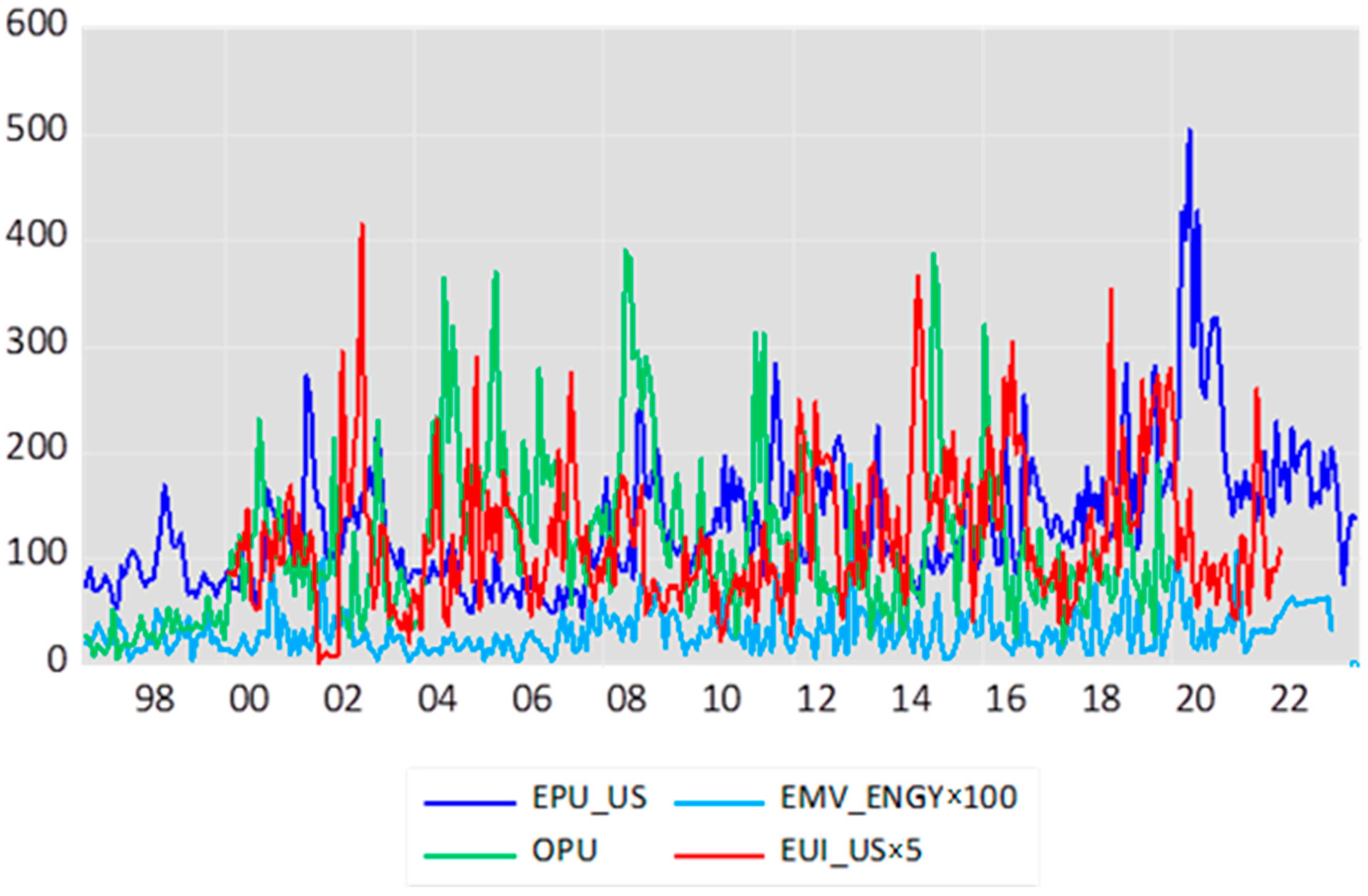
This study employs several measures to proxy uncertainty in the energy sector, including the EPU, EMV calibrated to energy policy (EMV_E), oil price uncertainty (OPU), and energy uncertainty index (EUI). Figure 1 shows a time series plots of the uncertainty indices. The volatility/uncertainty series reaches top by OPU (76.92), followed by EPU_US (63.86). The figures show the EPU_US spike in May 2020 (503.96), and the OPU in June 2008 (390.43) (These figures were taken from the high points of each time series path and were not reported). The correlations between these series are not obvious from the chart.

Table 3. Correlations for various measures of uncertainty.

	EPU	EMVE	OPU	EUI	CPU
EPU	1
	-----
EMVE	0.314	1
	5.10	-----
OPU	−0.138	0.114	1
	−2.15	1.77	-----
EUI	0.104	−0.057	−0.036	1
	1.61	−0.88	−0.56	-----
CPU	0.501	0.122	−0.090	0.123	1
	8.93	1.89	−1.40	1.92	-----

Notes: Uncertainty variables include Economic policy uncertainty (EPU), Energy policy regulation induced stock market volatility (EMV_E), Oil price uncertainty (OPU), Energy uncertainty index (EUI), and Climate policy uncertainty (CPU). For each variable, the first row reports the estimated correlation coefficients, the second row contains the estimated t-statistics.

provides correlation analysis. It is apparent that, with the exceptions of the correlations between EPU and EMV_ENGY, EPU and OPU, and EPU and CPU, the correlations for other pairs are low, indicating that each uncertainty factor does not share much common information. However, the CPU series is nonstationary and taking the first difference in the natural logarithm denoted by ${∆cpu}_t$ is relevant. Thus, including ${∆cpu}_t$ along with other uncertainty variables simultaneously into a test equation may enhance the explanation of stock returns without suffering the multicollinearity problem.

5. Empirical Evidence

5.1. Empirical Results

The estimates of Equation (2), in conjunction with Equations (3) and (4), by adding the dummy variable from 2008-09 global financial crisis (GFC) and the 2019-20 infectious disease (ID), known as COVID-19, by applying GED-GARCH procedure, are reported in

Table 4. Estimates of U.S. sectoral stock returns in response to EPU, EMV, OPU, and EUI.

Variables	$\mathbf{Sec}\mathbf{toral}\mathbf{Stock}\mathbf{Returns}\left({\mathit{R}}_{\mathit{t}}\right)$
	ENGY	BMAT	CDIS	CSTP	FINA	HLTH	INDU	RLES	TECH	TELE	UTLI
C	5.090	5.584	2.691	2.276	4.466	2.302	4.564	4.351	4.072	0.652	2.174
	10.96	11.50	13.58	21.38	12.37	27.71	12.03	11.00	8.46	2.30	9.05
${EPU}_t$	−0.017	−0.018	−0.003	−0.004	−0.009	−0.002	−0.012	−0.005	−0.014	0.000	−0.005
	−6.19	−5.73	−1.53	−4.28	−4.19	−2.30	−5.79	−1.98	−5.93	−35.63	−3.18
${EMV}_{E,t}$	−1.082	−0.712	−0.520	−0.215	−2.106	−1.781	−2.191	−3.675	−1.228	−3.094	−0.295
	−13.87	−2.15	−2.16	−1.67	−4.42	−5.08	−6.02	−9.06	−2.63	−6.40	−17.68
${OPU}_t$	−0.010	−0.016	−0.006	−0.001	−0.012	−0.003	−0.011	−0.003	−0.016	0.000	0.004
	−6.66	−8.58	−11.23	−1.70	−7.62	−6.12	−6.75	−3.01	−11.42	14.42	5.22
${EUI}_t$	−0.027	−0.022	−0.026	−0.027	−0.021	−0.007	−0.013	−0.044	0.021	0.024	−0.037
	−4.16	−3.09	−4.11	−43.20	−2.79	−3.35	−7.88	−5.08	3.00	4.18	−7.68
${DUM}_t$	−0.377	−4.132	−7.342	−2.930	−0.717	−1.354	−5.249	−0.165	−0.829	−1.253	−3.781
	−3.51	−13.30	−33.11	−10.54	−1.14	−1.66	−2.45	−3.28	−0.70	−0.61	−8.41
$\omega$	23.055	23.457	8.657	7.667	19.501	9.019	4.248	3.817	33.830	15.891	32.909
	0.29	0.57	0.35	0.14	0.41	0.25	0.46	0.70	0.32	0.34	0.22
${\epsilon }_{t-1}^2$	0.218	0.610	0.635	0.233	1.780	0.216	0.417	0.231	0.213	1.328	4.474
	0.17	0.71	0.58	0.27	0.59	0.35	0.84	0.95	0.34	0.57	0.49
${\sigma }_{t-1}^2$	0.903	0.654	0.803	0.889	0.794	0.774	0.83	0.79	0.757	0.797	0.857
	3.42	1.52	2.1	1.33	2.7	0.99	3.84	3.74	1.06	2.35	2.9
${\overline{R}}^2$	0.04	0.07	0.00	0.04	0.06	0.03	0.07	0.03	0.02	0.00	0.05

Notes: The dependent variable is stock return ($R_t).$ For each model, the first row reports the estimated coefficients, the second row contains the estimated z-statistics. The critical values of z-distribution at the 1%, 5%, and 10% levels of significance are 2.58, 1.96, and 1.65, respectively. The 0.000 denotes a very small number. ${\overline{R}}^2$ is the adjusted R-squared for the coefficient of determination.

(The use of a dummy variable to capture the impacts of GFC and COVID-19 interruptions is required as Baker et al. [12] documented in their findings that the COVID-19 shock increased the VIX by about 500% from 15 January 2020 to 31 March 2020). The values in the first row are the estimated coefficients, and the values in the second row are the z-statistics. The estimates reveal several empirical results. First, the estimated coefficients of ${EPU}_t$ are statistically significant, indicating a harmful effect on stock markets as EPU increases. This effect stems from an increase in EPU, which adds uncertainty to business operation and thereby delays production. These results are consistent with the studies of [16,23,29], which showed that uncertainty shocks impede macroeconomic activity and private investment. This deterioration in investment decisions would cause firms’ future cash flows to decline, leading to a dip in stock returns.

Second, the coefficients of ${EMV}_{E,t}$ are negative and highly significant. The negative sign of the coefficient reflects market behavior in which shocking news emerging from energy regulation induced volatility in equity markets leads to deteriorating market expectations. Fears of a worsening in the stock market are likely to induce traders to sell their stocks, leading to a decline in returns. The evidence is consistent with the result reported by Chiang [69].

Third, evidence indicates that the ${OPU}_t$ has a negative effect on stock returns across different sectors, with the only exception being the Utility sector. This negative effect is expected, as a rise in ${OPU}_t$ impacts not only household consumption and firms’ real option decisions [36]. The resulting delay in investment decisions can lead to setbacks in production and declines in stock prices. The results are in line with the findings of Abiad and Qureshi [13].

For a rational investor, the focus of their investments is more likely on real stock return, which is measured by subtracting the inflation rate from the nominal stock return, $r_t$. The test equation can be rewritten as follows:

$$r_t=C+{\beta }_1{EPU}_t+{\beta }_2{EMV}_{E,t}+{\beta }_3{OPU}_t+{\beta }_4{EUI}_t+{\beta }_5{DUM}_t+{\epsilon }_t$$

(6)

Table 5. Estimates of U.S. sectoral real stock returns in response to EPU, EMV, OPU, and EUI.

Variables	$\mathbf{Sec}\mathbf{toral}\mathbf{Real}\mathbf{Stock}\mathbf{Returns}({\mathit{r}}_{\mathit{t}}$)
	ENGY	BMAT	CDIS	CSTP	FINA	HLTH	INDU	RLES	TECH	TELE	UTLI
C	4.916	5.456	2.499	2.089	4.283	4.395	4.142	3.930	0.542	1.982	4.916
	12.25	14.10	14.86	55.96	12.97	11.27	17.95	8.46	7.38	8.81	12.25
${EPU}_t$	−0.017	−0.018	−0.003	−0.004	−0.009	−0.012	−0.005	−0.013	−0.001	−0.005	−0.017
	−7.47	−7.67	−1.71	−15.95	−3.91	−4.45	−3.64	−4.87	−3.09	−3.14	−7.47
${EMV}_{E,t}$	−0.994	−0.645	−0.564	−0.250	−2.064	−2.206	−3.700	−1.185	−4.049	−0.391	−0.994
	−14.20	−9.28	−2.13	−2.38	−3.81	−4.10	−7.54	−1.88	−59.94	−9.67	−14.20
${OPU}_t$	−0.010	−0.016	−0.006	−0.001	−0.011	−0.010	−0.003	−0.016	0.004	0.004	−0.010
	−5.51	−10.67	−7.99	−1.98	−6.96	−6.10	−7.88	−9.25	15.27	4.07	−5.51
${EUI}_t$	−0.027	−0.018	−0.025	−0.028	−0.020	−0.013	−0.046	0.022	0.018	−0.038	−0.027
	−5.15	−5.96	−4.01	−11.95	−5.52	−5.34	−6.48	2.58	11.10	−8.63	−5.15
${DUM}_t$	−2.593	−4.321	−7.345	−2.905	−0.877	−5.212	−0.113	−0.301	−1.094	−3.485	−2.593
	−1.79	−1.76	−21.52	−7.44	−0.47	−2.36	−6.65	−1.49	−2.59	−4.42	−1.79
$\omega$	27.395	29.683	11.841	6.889	15.697	5.321	4.952	7.872	7.654	11.633	27.395
	0.26	0.48	0.20	0.19	0.54	0.52	0.62	0.42	0.42	0.30	0.26
${\epsilon }_{t-1}^2$	0.171	1.004	0.220	0.334	1.087	0.494	0.304	0.698	0.875	0.774	0.171
	0.18	0.67	0.32	0.34	0.67	0.92	0.86	0.69	0.75	0.49	0.18
${\sigma }_{t-1}^2$	0.832	0.656	0.921	0.857	0.706	0.778	0.786	0.822	0.751	0.858	0.832
	1.43	1.38	2.84	1.48	2.07	3.13	3.29	3.55	2.51	2.77	1.43
${\overline{R}}^2$	0.05	0.07	0.00	0.04	0.06	0.07	0.03	0.02	0.01	0.05	0.05

Notes: The dependent variable is real stock return ($r_t=R_t-{∆p}_t).$ Independent variables are: Economic policy uncertainty (EPU), Energy policy regulation induced stock market volatility (EMV_E), Oil price uncertainty (OPU), Energy uncertainty index (EUI). Sectoral data includes Energy and Oil (ENGY), Basic Materials (BMAT), Consumer Discretionary (CDIS), Consumer Staples (CSTP), Financials (FINA), Health Care (HLTH), Industrials (INDU), Real Estate (RLES), Technology (TECH), Telecommunications (TELE), and Utilities (UTLI). For each model, the first row reports the estimated coefficients, the second row contains the estimated z-statistics. The critical values of z-distribution at the 1%, 5%, and 10% levels of significance are 2.58, 1.96, and 1.65, respectively. ${\overline{R}}^2$ is the adjusted R-squared for the coefficient of determination.

reports the estimates of Equation (6) using real stock return as the dependent variable. The test results are very comparable. That is, coefficients of ${EPU}_t$, ${EMV}_{E,t}$, ${OPU}_t$, and ${EUI}_t$ are all negative and statistically significant, with minor exceptions in the RLES, TECH, and TELE sectors.

For mean-variance investors, excess returns are expected if an investment is made on a risky asset such as stocks vs. fixed income. To address this issue, the excess stock return, which subtracts the risk-free interest rate (one-month Treasury bill rate, $i_t$) from the stock return, is used as the dependent variable.

Table 6. Estimates of U.S. sectoral excess stock returns in response to EPU, EMV, OPU, and EUI.

Variables	$\mathbf{Sec}\mathbf{toral}\mathbf{Excess}\mathbf{Stock}\mathbf{Returns}({\mathit{R}}_{\mathit{t}}-{\mathit{i}}_{\mathit{t}}$)
	ENGY	BMAT	CDIS	CSTP	FINA	HLTH	INDU	RLES	TECH	TELE	UTLI
C	5.317	6.617	3.491	2.818	4.305	2.696	4.675	4.371	4.000	1.452	1.592
	17.55	14.31	29.87	8.46	10.61	9.90	17.46	117.91	8.43	5.39	18.81
${EPU}_t$	−0.017	−0.020	−0.005	−0.006	−0.008	−0.010	−0.010	−0.005	−0.015	−0.001	−0.004
	−6.94	−6.74	−2.67	−2.97	−3.17	−6.17	−4.09	−9.88	−4.27	−5.61	−4.23
${EMV}_{E,t}$	−1.559	−1.583	−1.502	−0.335	−2.742	−0.005	−2.660	−4.051	−2.124	−3.150	−0.300
	−3.27	−3.92	−4.32	−2.81	−5.18	−4.25	−5.76	−43.02	−4.85	−8.25	−1.39
${OPU}_t$	−0.010	−0.016	−0.006	−0.002	−0.011	−1.858	−0.010	−0.003	−0.013	−0.003	0.004
	−5.82	−9.49	−5.77	−2.39	−7.56	−4.92	−23.91	−26.97	−6.46	−2.06	5.36
${EUI}_t$	−0.025	−0.025	−0.032	−0.031	−0.017	−0.007	−0.022	−0.044	0.007	0.011	−0.025
	−3.76	−3.20	−4.63	−9.17	−3.04	−2.77	−5.25	−18.75	4.77	3.57	−8.79
${DUM}_t$	−0.370	−4.207	−6.936	−2.590	−0.855	0.010	−5.605	2.846	−2.103	−1.349	−2.230
	−3.88	−6.02	−10.00	−13.64	−2.17	11.69	−25.04	24.14	−1.07	−0.67	−1.98
$\omega$	21.865	38.912	10.878	6.484	13.373	8.374	6.070	8.546	15.845	23.088	14.952
	0.33	0.65	0.39	0.31	0.58	0.42	0.54	0.45	0.51	0.30	0.31
${\epsilon }_{t-1}^2$	0.207	0.873	0.312	0.173	0.812	0.354	0.516	0.671	1.004	1.341	1.067
	0.16	0.71	0.54	0.24	0.66	0.41	0.85	0.73	0.65	0.50	0.50
${\sigma }_{t-1}^2$	0.908	0.476	0.682	0.832	0.697	0.782	0.741	0.815	0.644	0.799	0.793
	3.77	0.83	1.00	1.65	1.87	1.74	2.50	3.28	1.46	1.83	1.77
${\overline{R}}^2$	0.05	0.09	0.03	0.06	0.07	0.02	0.08	0.02	0.04	0.01	0.03

Notes: The dependent variable is excess stock return ($R_t-i_t).$ Independent variables are: Economic policy uncertainty (EPU), Energy policy regulation induced stock market volatility (EMV_E), Oil price uncertainty (OPU), Energy uncertainty index (EUI). Sectoral data includes Energy and Oil (ENGY), Basic Materials (BMAT), Consumer Discretionary (CDIS), Consumer Staples (CSTP), Financials (FINA), Health Care (HLTH), Industrials (INDU), Real Estate (RLES), Technology (TECH), Telecommunications (TELE), and Utilities (UTLI). For each model, the first row reports the estimated coefficients, the second row contains the estimated z-statistics. The critical values of z-distribution at the 1%, 5%, and 10% levels of significance are 2.58, 1.96, and 1.65, respectively. ${\overline{R}}^2$ is the adjusted R-squared for the coefficient of determination.

reports the estimates using excess stock return ($R_t-i_t)$ as the dependent variable for estimating each sector’s equation. The estimated results are robust, as the statistics demonstrate that the performance across different sectors produce very comparable qualitative results. The RLES and UTIL sectors are more sensitive to the dependent variable measure. However, the test results allow us to conclude that, in general, the ${EPU}_t$, ${EMV}_{E,t}$, ${OPU}_t$, and ${EUI}_t$ have significant adverse effects on stock returns, with only a couple of cases involving an unexpected sign. Evidence shows that the coefficients of the TECH and TELE sectors for the ${EUI}_t$ variable are positive, which can be used to hedge against the rise in uncertainty because less weight is placed on the energy use in its operations.

5.2. Evidence of Energy Prices Changes

5.2.1. Impact of Energy Uncertainty Index and Crude Oil Prices Changes

The impact of energy-related prices on stock returns is excluded in the above analyses. A frequently raised question is whether a rise in energy commodity prices will positively affect stock prices. Economically, this effect depends on how commodity prices in different sectors respond to input prices when using energy, which in turn depends on the price elasticity and the substitutability of energy alternatives. In an econometric sense, it may be contingent on the magnitude of the correlations. To examine the parametric effect, we introduce changes in crude oil price expressed in natural logarithm (${∆p}_{Oil,t}$) into the model. Thus, the regression model can be expressed as follows:

$$R_t=C+{\beta }_1{EPU}_t+{\beta }_2{EMV}_{E,t}+{\beta }_3{OPU}_t+{\beta }_4{EUI}_t+{\beta }_5{∆p}_{Oil.t}+{\beta }_6{DUM}_t+{\epsilon }_t$$

(7)

The estimates in

Table 7. Estimates of U.S. sectoral stock returns respond to various measures of uncertainties and crude oil price changes.

Variables	$\mathbf{Sec}\mathbf{toral}\mathbf{Stock}\mathbf{Returns}({\mathit{R}}_{\mathit{t}}$)
	ENGY	BMAT	CDIS	CSTP	FINA	HLTH	INDU	RLES	TECH	TELE	UTLI
C	2.042	3.740	2.239	1.981	4.157	2.116	3.528	4.235	2.505	0.241	1.868
	7.66	32.98	28.38	13.32	11.87	15.77	14.66	57.80	6.40	0.83	10.85
${EPU}_t$	−0.006	−0.012	0.000	−0.003	−0.008	−0.002	−0.008	−0.005	−0.009	0.001	−0.004
	−2.97	−8.19	−5.96	−2.00	−3.03	−6.79	−3.91	−5.17	−2.94	1.53	−4.90
${EMV}_{E,t}$	−1.386	−0.581	−0.662	−0.278	−2.089	−1.784	−2.243	−3.768	−1.567	−2.405	−0.379
	−3.10	−2.39	−2.28	−2.64	−3.95	−24.86	−4.34	−15.16	−2.10	−7.44	−2.90
${OPU}_t$	−0.001	−0.011	−0.006	0.000	−0.011	−0.003	−0.008	−0.004	−0.012	−0.001	0.005
	−3.48	−9.02	−19.68	6.47	−6.21	−7.28	−26.50	−5.37	−6.28	−1.67	4.97
${EUI}_t$	−0.010	−0.011	−0.010	−0.026	−0.018	−0.007	−0.008	−0.044	0.027	0.025	−0.036
	−11.65	−2.36	−6.25	−10.67	−2.53	−3.73	−11.69	−21.06	4.28	7.22	−10.26
${∆p}_{Oil.t}$	0.325	0.233	0.059	0.023	0.035	0.018	0.106	0.005	0.137	0.032	0.029
	35.96	16.65	18.51	3.42	3.39	6.32	16.85	1.45	18.19	11.70	4.84
${DUM}_t$	−3.676	−8.487	−6.048	−2.490	2.647	−1.833	−3.386	0.146	−1.303	−1.625	−2.985
	−2.39	−8.34	−27.90	−4.04	4.79	−3.11	−1.33	0.70	−0.67	−9.23	−6.69
$\omega$	15.847	15.271	10.708	7.595	12.737	9.766	8.301	12.196	10.818	17.915	10.019
	0.17	0.48	0.20	0.11	0.55	0.22	0.48	0.44	0.44	0.35	0.34
${\epsilon }_{t-1}^2$	0.232	0.710	0.266	0.227	0.713	0.306	0.997	0.680	1.177	1.460	1.207
	0.29	0.68	0.34	0.26	0.66	0.30	0.87	0.65	0.80	0.58	0.58
${\sigma }_{t-1}^2$	0.885	0.729	0.905	0.894	0.730	0.897	0.686	0.812	0.690	0.754	0.800
	1.71	1.95	2.32	1.15	2.11	2.56	1.97	2.82	2.05	1.92	2.35
${\overline{R}}^2$	0.31	0.11	0.01	0.04	0.01	0.03	0.11	0.03	0.06	0.00	0.05

Notes: The dependent variable is stock return for sector i ($R_t).$ Independent variables are: Economic policy uncertainty (EPU), Energy policy regulation induced stock market volatility (EMV_E), Oil price uncertainty (OPU), Energy uncertainty index (EUI), and change of West Texas Intermediate (WTI) oil price in natural logarithm (${∆p}_{Oil,t})$. Independent variables are: Economic policy uncertainty (EPU), Energy policy regulation induced stock market volatility (EMV), Oil price uncertainty (OPU), energy uncertainty index (EUI), and changes in WTI oil price, ${∆p}_{Oil,t}$. Sector i refers to Energy and Oil (ENGY), Basic Materials (BMAT), Consumer Discretionary (CDIS), Consumer Staples (CSTP), Financials (FINA), Health Care (HLTH), Industrials (INDU), Real Estate (RLES), Technology (TECH), Telecommunications (TELE), and Utilities (UTLI). For each model, the first row reports the estimated coefficients, the second row contains the estimated z-statistics. A similar result is achieved by using the Blent crude oil price change, ${∆p}_{Oil.t}$. The critical values of z-distribution at the 1%, 5%, and 10% levels of significance are 2.58, 1.96, and 1.65, respectively. ${\overline{R}}^2$ is the adjusted R-squared for the coefficient of determination.

and

Table 8. Estimates of U.S. sectoral stock returns respond to various measures of uncertainties and gasoline price changes.

Variables	$\mathbf{Sec}\mathbf{toral}\mathbf{Stock}\mathbf{Returns}({\mathit{R}}_{\mathit{t}}$)
	ENGY	BMAT	CDIS	CSTP	FINA	HLTH	INDU	RLES	TECH	TELE	UTLI
C	2.852	4.376	2.401	2.034	4.439	2.010	3.840	4.433	2.550	0.426	1.665
	10.28	22.17	13.21	12.87	12.01	21.35	12.07	22.17	7.25	1.73	9.64
${EPU}_t$	−0.009	−0.013	−0.002	−0.003	−0.009	−0.001	−0.008	−0.005	−0.008	0.000	−0.003
	−6.94	−8.34	−1.90	−5.52	−4.34	−2.19	−4.29	−3.29	−2.54	2.33	−2.30
${EMV}_{G,t}$	−0.830	−0.418	−0.523	−0.167	−2.087	−1.731	−1.802	−3.661	−1.337	−2.431	−0.287
	−2.29	−8.53	−1.88	−1.87	−4.47	−7.83	−3.64	−6.63	−7.82	−6.06	−7.22
${OPU}_t$	−0.005	−0.013	−0.005	−0.001	−0.012	−0.002	−0.009	−0.003	−0.011	−0.002	0.005
	−4.19	−21.47	−9.81	−6.46	−7.75	−3.46	−6.58	−5.71	−5.92	−3.59	8.98
${EUI}_t$	−0.012	−0.009	−0.023	−0.025	−0.021	−0.006	−0.006	−0.044	0.024	0.024	−0.035
	−2.91	−5.89	−4.55	−9.45	−2.71	−1.70	−4.04	−7.84	2.96	5.34	−7.89
${∆p}_{Gasl.t}$	0.166	0.097	0.021	0.016	0.001	0.021	0.055	−0.007	0.068	0.012	0.032
	18.69	10.65	3.76	2.22	6.21	6.14	8.36	−2.79	10.15	2.84	4.78
${DUM}_t$	−3.310	−6.668	−6.932	−2.666	−0.661	−3.185	−4.566	−0.169	−3.022	−1.368	−2.808
	−1.89	−3.05	−12.51	−4.35	−2.40	−3.86	−1.81	−1.84	−1.99	−0.62	−2.87
$\omega$	18.554	18.660	12.282	7.128	20.733	9.398	12.448	4.428	7.175	102.064	11.938
	0.20	0.46	0.19	0.14	0.41	0.20	0.46	0.61	0.48	0.23	0.34
${\epsilon }_{t-1}^2$	0.196	0.787	0.298	0.183	1.829	0.196	0.835	0.276	0.776	7.611	1.527
	0.18	0.67	0.34	0.22	0.57	0.26	0.75	0.88	0.82	0.43	0.57
${\sigma }_{t-1}^2$	0.905	0.729	0.939	0.861	0.789	0.869	0.727	0.800	0.746	0.813	0.795
	2.69	1.87	4.09	0.97	2.60	1.62	1.92	3.58	2.80	1.83	2.32
${\overline{R}}^2$	0.18	0.10	0.01	0.04	0.05	0.04	0.08	0.03	0.04	0.00	0.05

Notes: The dependent variable is stock return for sector i ($R_t).$ Independent variables are: Economic policy uncertainty (EPU), petroleum markets policy induced stock market volatility (EMV_G), Oil price uncertainty (OPU), Energy uncertainty index (EUI) and changes in gasoline price, ${∆p}_{Gasl,t}$. Sector i refers to Energy and Oil (ENGY), Basic Materials (BMAT), Consumer Discretionary (CDIS), Consumer Staples (CSTP), Financials (FINA), Health Care (HLTH), Industrials (INDU), Real Estate (RLES), Technology (TECH), Telecommunications (TELE), and Utilities (UTLI). For each model, the first row reports the estimated coefficients, the second row contains the estimated z-statistics. The critical values of z-distribution at the 1%, 5%, and 10% levels of significance are 2.58, 1.96, and 1.65, respectively. The 0.000 denotes a very small number. ${\overline{R}}^2$ is the adjusted R-squared for the coefficient of determination.

reflect the inclusion of changes in oil prices as new ingredients (However, our interest is focusing on the contemporaneous period to avoid the over parametrization, but the current model contains more uncertainty variable than the VIX alone. When adding lagged effects on the explanatory variables, just follow Dixit and Pindyck [58]). The estimates in Table 7 are based on the West Texas Intermediate (WTI) to measure ${∆p}_{Oil.t}$. A similar result was achieved by using Brent crude oil price (not reported). Several points deserve our attention. First, the four major uncertainty variables, including ${EPU}_t$, ${EMV}_{E,t}$, ${OPU}_t$, and ${EUI}_t$, consistently produce comparable results for both the estimated coefficients and the responding significant levels, suggesting that the test equations are not significantly disturbed by the addition of new price change variables. Furthermore, the negative coefficients indicate that energy uncertainty tends to produce adverse effects on stocks. However, the coefficients of ${OPU}_t$ in UTLI and the slopes of ${EUI}_t$ in TECH and TELE sectors are present positive signs, suggesting their capacity to hedge against energy uncertainties. Note that the simultaneous significance of uncertainty factors measured by ${EPU}_t$, ${EMV}_{E,t}$, ${OPU}_t$, and ${EUI}_t$ also implies that there is no redundant information and that they broadly cover different dimensions of explanatory power in describing sectoral stock returns, as reflected by the low correlation among these uncertainty variables.

Second, the coefficients of ${∆p}_{Oil.t}$ are positive and statistically significant, except in the RLES sector, which is statistically insignificant. The positive coefficients for ${∆p}_{Oil.t}$ suggest that oil-related companies can immediately account for the price effect on their current and future cash flows based on the present value model [8]. This finding is consistent with the study by El-Sharif et al. [36], who examined the relationship between changes in oil prices and stock returns in the UK oil and gas sector. They reported that the relationship between the two variables was significantly positive. Our evidence shows that stock price returns can absorb a rise in oil prices in their commodity prices and turn out to be profitable. Part of the reason is that the demand elasticity for oil is relatively lower, which allows profit to rise even when the price is higher [37].

Third, all coefficients of dummy variables are negative and statistically significant, except for those in the FINA and RLES sectors, which are positive. This finding suggests that the inclusion of the dummy variable for controlling unusual observations helps mitigate the bias arising from sharp disturbance in the time series estimations.

5.2.2. Robustness Checks for Gasoline Price Changes

In this section, we conduct robustness tests by replacing energy-induced EMV (${EMV}_{E,t}$) with petroleum market policy-induced EMV (${EMV}_{G,t}$); at the same time, the ${∆p}_{Oil.t}$ is replaced by ${∆p}_{Gasl,t}$ which is the change in gasoline price expressed in natural logarithm. Estimates with these adjustments for explanatory variables are reported in Table 8. There are two key findings. First, with respect to the coefficients of ${EPU}_t$, ${EMV}_{G,t}$, ${OPU}_t$, and ${EUI}_t$, the statistics consistently display comparable results for both the estimated coefficients and the significance level, as shown in Table 8. Note that the findings of negative relation of the petroleum markets uncertainty (${EMV}_{G,t}$) and stock returns are consistent with the result reported by Kang et al. [11]. The coefficients of ${OPU}_t$ in the UTIL sector and ${EUI}_t$ in the TECH and TELE sectors exhibit opposite signs, as reported in Table 8. The evidence clearly indicates that the parameters are stable across different uses of the explanatory variables.

Second, the coefficients for the ${∆p}_{Gasl,t}$ in Table 8 are positive and maintain a high level of significance for 10 of 11 sectors. However, the RLES sector exhibits a negative sign, indicating incompetence to hedge against gasoline price inflation. This suggests that a rise in gasoline prices tends to have a harmful effect on portfolio holders of the RLES sector. However, evidence indicates a positive association between stock returns and changes in gasoline prices for most sectors, which is consistent with market conditions that are commonly correlated with other economic variables. Bernanke [70] provides a plausible explanation for the tendency for stocks and gasoline prices to move together, namely, that both are reacting to a common factor, namely, a softening of global aggregate demand, which hurts both corporate profits and demand for gasoline.

6. Evidence of Climate Policy Changes

6.1. Direct Effect of Climate Policy Changes

This section conducts an empirical investigation using changes in climate policy uncertainty (${∆cpu}_t$) to replace ${EPU}_t$, emphasizing the impact of climate change risk on stock returns. The ${∆cpu}_t$ is used because the original form of CPU_t is nonstationary. Additionally, the dummy variable is replaced with two volatile variables to capture unusual market conditions, including equity market volatility calibrated to financial crises (${EMV}_{FC,t}$) and infectious disease (${EMV}_{ID,t}$) series. The estimated results obtained by incorporating these elements are expressed as follows:

$$R_t=C+{\beta }_1{∆cpu}_t+{\beta }_2{EMV}_{E,t}+{\beta }_3{OPU}_t{+\beta }_4{EUI}_t+{\beta }_5{∆p}_{Gasl.t}{+\beta }_6{EMV}_{FC,t}+{\beta }_7{EMV}_{ID,t}+{\epsilon }_t$$

(8)

where $R_t$ in Equation (8) is the dependent variable for sectoral stock returns. The independent variables are: change in climate policy uncertainty in the natural logarithm (${∆cpu}_t$), energy policy regulation-induced equity market volatility (${EMV}_{E,t}$, oil price uncertainty (${OPU}_t$), energy uncertainty index (${EUI}_t$), and changes in gasoline price (${∆p}_{Gasl.t})$ controlling the equity market volatility calibrated to financial crises (${EMV}_{FC}$) and infectious diseases (${EMV}_{ID}$), respectively.

The estimates are presented in

Table 9. Estimates of U.S. sectoral stock returns respond to climate policy changes.

Variables	$\mathbf{Sec}\mathbf{toral}\mathbf{Stock}\mathbf{Returns}({\mathit{R}}_{\mathit{t}}$)
	ENGY	BMAT	CDIS	CSTP	FINA	HLTH	INDU	RLES	TECH	TELE	UTLI
C	1.775	3.199	2.497	2.077	4.285	2.402	3.418	4.285	1.644	1.489	2.251
	10.51	11.01	14.72	12.70	26.56	14.48	18.99	26.56	3.50	5.00	9.48
${∆cpu}_t$	−0.003	−0.029	−0.004	−0.001	−0.014	−0.007	−0.009	−0.014	−0.013	−0.006	−0.001
	−3.16	−7.63	−2.27	−3.10	−5.87	−5.07	−5.62	−5.87	−3.39	−2.42	−1.99
${EMV}_{E,t}$	−2.135	−1.342	−1.771	−1.186	−3.212	−2.290	−2.721	−3.212	−2.091	−1.784	−1.150
	−5.95	−2.32	−7.73	−3.07	−5.77	−8.19	−5.43	−5.77	−2.86	−2.89	−3.06
${OPU}_t$	0.004	−0.007	−0.004	0.001	−0.009	−0.002	−0.006	−0.009	−0.010	−0.002	0.005
	2.92	−8.61	−4.95	1.53	−13.78	−2.06	−4.39	−13.78	−3.51	−2.32	5.10
${EUI}_t$	−0.019	−0.005	−0.015	−0.024	−0.014	−0.004	−0.005	−0.014	0.045	0.021	−0.030
	−8.08	−0.62	−4.32	−6.14	−12.68	−1.17	−3.58	−12.68	3.52	2.30	−6.74
${∆p}_{Gasl.t}$	0.351	0.175	0.077	0.059	0.074	0.034	0.135	0.074	0.153	0.056	0.048
	59.10	21.35	13.72	14.16	11.22	4.57	15.65	11.22	7.47	3.96	6.16
${EMV}_{FC,t}$	−0.847	−1.791	−0.952	−0.721	−1.619	−0.929	−1.532	−1.619	−0.254	−1.331	−1.482
	−5.19	−10.75	−10.40	−6.97	−12.07	−6.34	−15.25	−12.07	−1.38	−5.36	−8.85
${EMV}_{ID,t}$	−0.018	0.004	0.073	−0.014	−0.010	0.024	−0.007	−0.010	0.059	−0.001	−0.030
	−9.29	0.55	6.17	−1.90	−1.04	1.37	−3.57	−1.04	1.86	−0.08	−2.97
$\omega$	42.687	16.311	61.107	7.842	10.439	9.967	12.076	10.439	4.615	14.321	7.406
	0.14	0.51	1.85	0.08	0.56	0.24	0.49	0.56	0.64	0.57	0.35
${\epsilon }_{t-1}^2$	17.506	0.699	2.973	0.181	0.996	0.271	1.294	0.996	0.451	0.518	0.976
	0.30	0.73	1.11	0.25	0.93	0.34	0.91	0.93	1.00	0.65	0.63
${\sigma }_{t-1}^2$	0.912	0.698	0.099	0.923	0.670	0.800	0.672	0.670	0.745	0.656	0.795
	2.72	1.83	0.84	1.25	2.17	1.12	1.89	2.17	3.37	1.45	2.46
${\overline{R}}^2$	0.38	0.17	0.06	0.05	0.12	0.05	0.16	0.12	0.08	0.03	0.05

Notes: The dependent variable is stock return for sector i ($R_t).$ Independent variables are: change in climate policy uncertainty in natural logarithm (${∆cpu}_t$), energy policy regulation induced stock market volatility ((${EMV}_{E,t}$, oil price uncertainty (${OPU}_t$), energy uncertainty index (${EUI}_t$), and changes in gasoline price (${∆p}_{Gasl.t})$ controlling the equity market volatility calibrated to financial crises (${EMV}_{FC,t}$) and infectious disease (${EMV}_{ID,t}$). Sector i refers to Energy and Oil (ENGY), Basic Materials (BMAT), Consumer Discretionary (CDIS), Consumer Staples (CSTP), Financials (FINA), Health Care (HLTH), Industrials (INDU), Real Estate (RLES), Technology (TECH), Telecommunications (TELE), and Utilities (UTLI). For each model, the first row reports the estimated coefficients, the second row contains the estimated z-statistics. The critical values of z-distribution at the 1%, 5%, and 10% levels of significance are 2.58, 1.96, and 1.65, respectively. The 0.000 denotes a very small number. ${\overline{R}}^2$ is the adjusted R-squared for the coefficient of determination.

. The coefficients of ${∆cpu}_t$ are negative and statistically significant across different sectors. The negative sign is consistent with our expectation that a rise in climate policy uncertainty will have a significant impact on energy volatility, and hence, equity market volatility that can produce fears and lower stock returns. The negative effect observed across different sectors can also be explained using a valuation model in which the net present value is negative due to discounting future income streams, less the costs of reducing emissions and social costs of carbon [34]. The evidence is consistent with the finding that the spillover effect of climate uncertainty on business production or household consumption causes ${∆cpu}_t$ uncertainty and financial instability, which negatively affect economic activity [68,71]. This finding is in line with Dutta et al. [60], who found that ${CPU}_t$ has a profound effect in triggering oil market fears and causing spillovers to other sectors. Moreover, these negative effects can be reinforced by unexpected climate-influenced sentiments, which can have an impact on decision-making and hence stock returns, as emphasized by Schulte-Huermann [72].

Evidence shows that the estimated coefficient for ${∆p}_{Gasl.t}$ is positive and highly significant, indicating that stock prices increase when gasoline prices rise. This trend is primarily attributable to the fact that rising gasoline prices being interpreted as a sign of a healthy economy with an increase in demand, which can positively influence stock market performance. This market phenomenon is consistent with the findings of Bernanke [70] and Kocaarslan and Soytas [73]. With respect to the performance of other uncertainty variables, such as $\{{EMV}_{E,t},{OPU}_t$, ${EUI}_t$, ${EMV}_{FC,t}$ and ${EMV}_{ID,t}\},$ evidence shows that the majority of these variables continually present negative signs. However, in some instances, the coefficients turn positive, which may be attributable to spurious correlations.

6.2. Interaction Between Changes in Oil Prices and Climate Policy Changes

The impart effect was ignored in the previous section on the interaction between oil price changes and climate policy changes. An increase in oil prices is mainly due to an advancement in economic activity, which is accompanied by the production of greenhouse gases (GHGs) from the combustion of fossil fuels, thus inducing the likelihood of government intervention in reducing emissions. The impact will cause an adverse effect on stock returns. By incorporating lagged variables, the model effectively captures the dynamic adjustment processes inherent in financial and policy transmission mechanisms. This approach allows us to reflect the fact that both policy responses and market adjustments typically unfold over time rather than instantaneously. Accordingly, the inclusion of the lagged interaction term ${∆cpu}_{t-1}{·∆p}_{oil.t-1}$ leads to a more accurate estimation of the cumulative and delayed impact of joint energy and climate policy shocks on sectoral stock returns. Thus, the product term ${∆cpu}_{t-1}{·∆p}_{oil.t-1}$ tends to have a negative effect on sectoral stocks. The estimates incorporating ${∆cpu}_{t-1}{·∆p}_{oil.t-1}$ into the model and replacing ${∆p}_{Gasl.t}$ with ${∆p}_{oil.t}$ are presented in

Table 10. Estimates of U.S. sectoral stock returns respond to the interaction between changes in oil prices and climate policy changes.

Variables	$\mathbf{Sec}\mathbf{toral}\mathbf{Stock}\mathbf{Returns}({\mathit{R}}_{\mathit{t}}$)
	ENGY	BMAT	CDIS	CSTP	FINA	HLTH	INDU	RLES	TECH	TELE	UTLI
C	1.263	2.521	2.024	1.608	3.103	1.883	2.455	3.292	1.708	0.666	1.187
	7.47	12.51	19.53	21.40	11.82	23.19	17.72	19.35	6.07	3.47	14.78
${∆cpu}_t$	−0.004	−0.009	−0.004	−0.003	−0.013	−0.007	−0.012	−0.005	−0.017	−0.006	−0.002
	−5.19	−6.77	−4.58	−8.75	−7.73	−5.87	−8.52	−2.31	−7.39	−8.69	−9.79
${∆cpu}_{t-1}{·∆p}_{oil.t-1}$	−0.003	−0.002	−0.001	−0.001	−0.001	−0.001	−0.001	0.001	−0.001	−0.001	−10.001
	−17.03	−10.79	−9.93	−9.52	−2.70	−8.23	−11.82	2.21	−7.93	−4.64	−2.12
${EMV}_{E,t}$	−2.450	−1.878	−1.315	−0.600	−2.487	−2.209	−2.821	−3.956	−1.773	−2.093	−0.790
	−19.71	−5.84	−4.46	−3.04	−5.23	−11.51	−5.66	−8.61	−3.30	−5.35	−2.73
${OPU}_t$	0.002	−0.008	−0.004	0.002	−0.009	−0.002	−0.006	−0.001	−0.010	−0.003	0.007
	1.78	−6.15	−8.28	9.30	−5.15	−5.23	−6.86	−0.85	−5.38	−3.48	6.99
${EUI}_t$	−0.010	−0.010	−0.017	−0.025	−0.021	−0.005	−0.005	−0.038	0.035	0.023	−0.032
	−6.76	−5.95	−7.50	−8.42	−3.87	−2.08	−7.56	−6.04	4.49	3.98	−16.62
${∆p}_{oil.t}$	0.373	0.206	0.077	0.049	0.080	0.041	0.142	0.057	0.143	0.060	0.043
	41.23	16.30	9.96	6.37	7.65	9.82	12.08	5.07	9.06	5.17	20.28
${EMV}_{FC,t}$	−4.519	−8.720	−7.235	−3.524	−0.654	−2.331	−4.888	−0.441	−3.865	−1.869	−2.513
	−2.84	−11.38	−11.62	−8.39	−0.32	−14.88	−2.06	−0.14	−4.91	−7.48	−2.91
${EMV}_{ID,t}$	−8.436	−1.454	−7.726	−4.450	−9.316	−0.850	−7.223	−4.192	2.198	−2.354	−5.891
	−9.86	−1.84	−5.28	−2.06	−6.66	−3.32	−8.02	−4.23	0.77	−1.27	−3.02
$\omega$	19.987	18.289	13.609	8.022	4.440	10.037	10.452	11.591	11.127	0.258	11.945
	0.28	0.49	0.21	0.12	0.59	0.22	0.50	0.56	0.49	0.38	0.30
${\epsilon }_{t-1}^2$	0.279	0.705	0.258	0.243	0.824	0.222	0.705	0.820	1.061	1.824	0.557
	0.40	0.66	0.35	0.27	0.78	0.23	0.70	0.78	0.84	0.57	0.45
${\sigma }_{t-1}^2$	0.871	0.709	0.896	0.889	0.691	0.913	0.716	0.717	0.708	0.726	0.858
	2.26	1.70	2.21	1.22	2.03	3.02	1.92	2.14	2.25	1.79	2.46
${\overline{R}}^2$	0.37	0.16	0.04	0.07	0.11	0.05	0.15	0.05	0.06	0.02	0.06

Notes: The dependent variable is stock return for sector i ($R_t).$ Independent variables are: change in climate policy uncertainty in natural logarithm (${∆cpu}_t$), interacting term $\mathrm{o}\mathrm{f}{∆cpu}_{t-1}·{∆p}_{oil.t-1},$ energy policy regulation induced stock market volatility ((${EMV}_{E,t}$), oil price uncertainty (${OPU}_t$), energy uncertainty index (${EUI}_t$), and changes in oil price (${∆p}_{oil.t})$ controlling the equity market volatility calibrated to financial crises (${EMV}_{FC,t}$) and infectious disease (${EMV}_{ID,t}$). Sector i refers to Energy and Oil (ENGY), Basic Materials (BMAT), Consumer Discretionary (CDIS), Consumer Staples (CSTP), Financials (FINA), Health Care (HLTH), Industrials (INDU), Real Estate (RLES), Technology (TECH), Telecommunications (TELE), and Utilities (UTLI). For each model, the first row reports the estimated coefficients, the second row contains the estimated z-statistics. The critical values of z-distribution at the 1%, 5%, and 10% levels of significance are 2.58, 1.96, and 1.65, respectively. The 0.000 denotes a very small number. ${\overline{R}}^2$ is the adjusted R-squared for the coefficient of determination.

.

The evidence presented in this table can be summarized as follows. First, the slopes of ${∆cpu}_t$ are uniformly negative and strongly significant. The negative signs are consistent with the hypothesis that a rise in climate policy uncertainty posits a fear that the government might raise taxes on the rise in emissions, which would give a downward pression on profits and hence stock returns. Second, the coefficient of the interacting term ${∆cpu}_{t-1}{\mathrm{a}\mathrm{n}\mathrm{d}∆p}_{oil.t-1}$ is negative and highly significant, confirming the observation that the feedback effect between ${∆cpu}_{t-1}{\mathrm{a}\mathrm{n}\mathrm{d}∆p}_{oil.t-1}$ produces an adverse impact on stock returns. The only exception is the real estate sector, where the evidence is positive. The evidence also implies that ${∆cpu}_t$ is not independent of ${∆p}_{oil.t.}$ Third, a related variable, ${EMV}_{E,t}$, which is energy- and environmental policy-induced volatility, exhibits a significantly negative impact on stock returns. This policy variable, ${EMV}_{E,t}$, along with ${∆cpu}_t,$ consistently presents robust effects compared with the other two variables, oil price uncertainty (${OPU}_t$) and energy uncertainty index (${EUI}_t$), because evidence in Table 10 reveals positive effects in some sectors for the latter two variables. Fourth, the coefficients of changes in oil prices consistently remain positive and highly significant, and the evidence is consistent with previous studies [5,37,74] across sectors after controlling for uncertainty factors.

7. Conclusions and Implications

This study examines sectoral stock returns in response to various measures of uncertainty, using monthly data from January 1997 to December 2023. This study has achieved several important empirical findings. First, evidence shows that stock returns in the energy sector are negatively correlated with ${∆cpu}_t$ ${EPU}_t$, ${EMV}_{E,t}$, ${OPU}_t,$ and ${EUI}_t;$ this holds true for the estimations of other sectors, suggesting that these uncertainty factors adversely affect sectoral stock returns. Although both ${OPU}_t$ and ${EUI}_t$ contain elements of energy-related uncertainty, they have different informational content and appear to complement each other when explaining the stock return equations. The finding that oil price uncertainty negatively affects stock returns is consistent with the result provided by Joo and Park [75]. As expected, there are minor exceptions, and reverse signs are found in the slope of OPU in the RLES sector and in the coefficients of EUI in the TECH and TELE sectors.

Second, changes in energy-related commodity prices, including ${∆p}_{Oil.t}$ and ${∆p}_{Gasl,t}$, have a significantly positive effect in explaining sectoral stocks, except in the RLSE sector. The positive coefficients for changes in energy-related prices imply that sectoral stock returns have a significant ability to hedge against upward shifts in energy-related prices. These findings are consistent with the literature [3,76,77,78]. However, this study reveals significant uncertainty factors that appear to provide incremental efficiency in explaining how sectoral factors affect stock returns.

Third, evidence derived from this study consistently shows that the coefficients of change in climate policy uncertainty reveal negative signs; this result holds true for all sectors as investors perceive that climate policy change could harm economic activity and raise carbon costs that tend to jeopardize their future stock performance, leading to a negative response to climate policy. Further, this study finds that changes in climate policy uncertainty interact with changes in oil prices, reflecting the government’s intention to use policy to curb rising carbon emissions produced by burning fuels to advance economic activity. The interaction between changes in climate policy uncertainty and changes in oil prices caused stock prices to plummet.

Fourth, the empirical analysis identifies that extreme observations during the 2008 global financial crisis and the 2020–2021 COVID-19 pandemic periods have significant downturn effects [31]. To mitigate bias in estimations, this study employs a dummy variable approach or conditional volatility to control the two periods.

Finally, this study offers practical implications. It identifies several uncertainty variables, including general economic uncertainty (${EPU}_t$), energy- or gasoline-induced equity market volatility ((${EMV}_{E,t}$), oil price uncertainty (${OPU}_t$), and the energy uncertainty index (${EUI}_t$), change in climate policy uncertainty (${∆cpu}_t)$ and its interaction with oil prices, and volatilities arising from the 2008 financial crisis (${EMV}_{FC,t}$), as well as the infectious diseases of 2020 (${EMV}_{ID,t}$). Each of these factors exerts a significantly negative effect on sectoral stock returns. As a result, these uncertainty measures can serve as complementary variables in explaining stock return behavior. These findings have meaningful implications for investors, regulators, and financial analysts. For investors, incorporating these forward-looking uncertainty variables into asset allocation and risk management models may enhance sector-specific performance forecasting. For policymakers, the evidence underscores the destabilizing potential of climate- and energy-related policy ambiguity on financial markets. Transparent communication and regulatory consistency may help mitigate such volatility. Moreover, this study suggests that the identification of these uncertainty variables should be priced in stock returns, although they serve as control variables when assessing the relationship between stock prices and energy prices. Omitting them in empirical specifications may lead to biased estimations. Integrating these uncertainty measures into valuation and stress-testing frameworks offers a more comprehensive approach to understanding market dynamics amid energy transition and climate-related risks.

References

1. Hammoudeh, S.; Li, H. Oil sensitivity and systematic risk in oil-sensitive stock indices. J. Econ. Bus. 2005, 57, 1–21. [Google Scholar] [CrossRef]
2. Filis, G.; Degiannakis, S.; Floros, C. Dynamic correlation between stock market and oil prices: The case of oil-importing and oil-exporting countries. Int. Rev. Financ. Anal. 2011, 20, 152–164. [Google Scholar] [CrossRef]
3. Sadorsky, P. Risk factors in stock returns of Canadian oil and gas companies. Energy Econ. 2001, 23, 17–28. [Google Scholar] [CrossRef]
4. Boyer, M.M.; Filion, D. Common and fundamental factors in stock returns of Canadian oil and gas companies. Energy Econ. 2007, 29, 428–453. [Google Scholar] [CrossRef]
5. Nandha, M.; Faff, R. Does oil move equity prices? A global view. Energy Econ. 2008, 30, 986–997. [Google Scholar] [CrossRef]
6. Hamilton, J.D. Historical Oil Shocks; (NBER Working Paper 16790); NBER: Cambridge, MA, USA, 2011. [Google Scholar]
7. Hwang, I.; Kim, J. Oil price shocks and the US stock market: A nonlinear approach. J. Empir. Financ. 2021, 64, 23–36. [Google Scholar] [CrossRef]
8. Jones, C.M.; Kaul, G. Oil and the stock markets. J. Financ. 1996, 51, 463–491. [Google Scholar] [CrossRef]
9. Kilian, L. Not all oil price shocks are alike: Disentangling demand and supply shocks in the crude oil market. Am. Econ. Rev. 2009, 99, 1053–1069. [Google Scholar] [CrossRef]
10. Kilian, L.; Park, C. The impact of oil price shocks on the U.S. stock market. Int. Econ. Rev. 2009, 50, 1267–1287. [Google Scholar] [CrossRef]
11. Kang, W.; de Gracia, F.P.; Ratti, R.A. Oil price shocks, policy uncertainty, and stock returns of oil and gas corporations. J. Int. Money Financ. 2017, 70, 344–359. [Google Scholar] [CrossRef]
12. Baker, S.R.; Bloom, N.; Davis, S.J.; Terry, S.J. COVID-Induced Economic Uncertainty; (No. w26983); NBER: Cambridge, MA, USA, 2020. [Google Scholar]
13. Abiad, A.; Qureshi, I.A. The macroeconomic effects of oil price uncertainty. Energy Econ. 2023, 125, 106839. [Google Scholar] [CrossRef]
14. Dang, H.-N.; Nguyen, C.P.; Lee, G.S.; Nguyen, B.Q.; Le, T.T. Measuring the energy-related uncertainty. Energy Econ. 2023, 124, 106817. [Google Scholar] [CrossRef]
15. Diaz, E.M.; Molero, J.C.; de Gracia, F.P. Oil price volatility and stock returns in the G7 economies. Energy Econ. 2016, 54, 417–430. [Google Scholar] [CrossRef]
16. Liu, X.; Wang, Y.; Du, W.; Ma, Y. Economic policy uncertainty, oil price volatility and stock market returns: Evidence from a nonlinear model. N. Am. J. Econ. Financ. 2022, 62, 101777. [Google Scholar] [CrossRef]
17. Behera, C.; Rath, B.N. The interconnectedness between crude oil prices and stock returns in G20 countries. Resour. Policy 2024, 91, 104950. [Google Scholar] [CrossRef]
18. Le, T.H.; Luong, A.T. Dynamic spillovers between oil price, stock market, and investor sentiment: Evidence from the United States and Vietnam. Resour. Policy 2022, 78, 102931. [Google Scholar] [CrossRef]
19. Alsalman, Z. Oil price uncertainty and the US stock market analysis based on a GARCH-in-mean VAR model. Energy Econ. 2016, 59, 251–260. [Google Scholar] [CrossRef]
20. Kang, W.; Ratti, R.A. Oil shocks, policy uncertainty and stock market return. J. Int. Financ. Mark. Inst. Money 2013, 26, 305–318. [Google Scholar] [CrossRef]
21. Adekoya, O.B.; Oliyide, J.A.; Kenku, O.T.; Al-Faryan, M.A.S. Comparative response of global energy firm stocks to uncertainties from the crude oil market, stock market, and economic policy. Resour. Policy 2022, 79, 103004. [Google Scholar] [CrossRef]
22. Balcilar, M.; Gupta, R.; Kim, W.J.; Kyei, C. The role of economic policy uncertainties in predicting stock returns and their volatility for Hong Kong, Malaysia and South Korea. Int. Rev. Econ. Financ. 2019, 59, 150–163. [Google Scholar] [CrossRef]
23. Chiang, T.C. Economic policy uncertainty, risk and stock returns: Evidence from G7 stock markets. Financ. Res. Lett. 2019, 29, 41–49. [Google Scholar] [CrossRef]
24. Nusair, S.; Al-Khasawneh, J.A. Impact of economic policy uncertainty on stock markets of the G7 Countries: A nonlinear ARDL approach. J. Econ. Asymmetries 2022, 26, e00251. [Google Scholar] [CrossRef]
25. Batten, J.A.; Kinateder, H.; Kinateder, P.G.; Wagner, N.F. Hedging stocks with oil. Energy Econ. 2021, 93, 104422. [Google Scholar] [CrossRef]
26. Lin, B.; Bai, R. Oil prices and economic policy uncertainty: Evidence from global, oil importers, and exporters’ perspective. Res. Int. Bus. Financ. 2021, 56, 101357. [Google Scholar] [CrossRef]
27. Baker, S.R.; Bloom, N.; Davis, S.J.; Kost, K. Policy News and Stock Market Volatility; (NBER Working Paper 25720); NBER: Cambridge, MA, USA, 2021. [Google Scholar]
28. Gavriilidis, K. Measuring Climate Policy Uncertainty; SSRN: Rochester, NY, USA, 2021. [Google Scholar]
29. Baker, S.R.; Bloom, N.; Davis, S.J. Measuring Economic Policy Uncertainty. Q. J. Econ. 2016, 131, 1593–1636. [Google Scholar] [CrossRef]
30. Dixit, A.K.; Pindyck, R.S. Irreversible Investment; Princeton University Press: Princeton, NJ, USA, 1994. [Google Scholar]
31. Goodell, J.W. COVID-19 and finance: Agendas for future research. Financ. Res. Lett. 2020, 35, 101512. [Google Scholar] [CrossRef]
32. Cheema, M.A.; Faff, R.; Szulczyk, K.R. The 2008 global financial crisis and COVID-19 pandemic: How safe are the safe haven assets? Int. Rev. Financ. Anal. 2022, 83, 102316. [Google Scholar] [CrossRef] [PubMed]
33. Johnston, J.; DiNardo, J. Econometric Methods, 4th ed.; McGraw-Hill: Niew York, NY, USA, 1997. [Google Scholar]
34. Barnett, M.; Brock, W.A.; Hansen, L.P. Pricing uncertainty induced by climate change. Rev. Financ. Stud. 2020, 33, 1024–1066. [Google Scholar] [CrossRef]
35. Sadorsky, P. Oil price shocks and stock market activity. Energy Econ. 1999, 21, 449–462. [Google Scholar] [CrossRef]
36. El-Sharif, I.; Brown, D.; Burton, B.; Nixon, B.; Russell, A. Evidence on the nature and extent of the relationship between oil prices and equity values in the UK. Energy Econ. 2005, 27, 819–833. [Google Scholar] [CrossRef]
37. Ramos, S.B.; Veiga, H. Risk factors in oil and gas industry returns: International evidence. Energy Econ. 2011, 33, 525–534. [Google Scholar] [CrossRef]
38. Agarwalla, M.; Sahu, T.N.; Jana, S.S. Dynamics of oil price shocks and emerging stock market volatility: A generalized VAR approach. Vilakshan-XIMB J. Manag. 2021, 18, 106–121. [Google Scholar] [CrossRef]
39. Smith, R.; Narayan, P.K. What do we know about oil prices and stock returns? Int. Rev. Financ. Anal. 2018, 57, 148–156. [Google Scholar] [CrossRef]
40. Degiannakis, S.; Filis, G.; Arora, V. Oil prices and stock markets. Energy J. 2018, 39, 85–130. [Google Scholar] [CrossRef]
41. Kling, J.L. Oil price shocks and stock market behavior. J. Portfolio Manag. 1985, 12, 34–39. [Google Scholar] [CrossRef]
42. Park, J.; Ratti, R. Oil price shocks and stock markets in the U.S. and 13 European countries. Energy Econ. 2008, 30, 2587–2608. [Google Scholar] [CrossRef]
43. Maghyereh, A.; Awartani, B. Oil price uncertainty and equity returns: Evidence from oil importing and exporting countries in the MENA region. J. Financ. Econ. Policy 2016, 8, 64–79. [Google Scholar] [CrossRef]
44. Faff, R.W.; Brailsford, T.J. Oil price risk and the Australian stock market. J. Energy Financ. Dev. 1999, 4, 69–87. [Google Scholar] [CrossRef]
45. Cong, R.G.; Wei, Y.M.; Jiao, J.L.; Fan, Y. Relationships between oil price shocks and stock market: An empirical analysis from China. Energy Policy 2008, 36, 3544–3553. [Google Scholar] [CrossRef]
46. Caporable, G.M.; Ali, F.M.; Spagnolo, N. Oil price uncertainty and sectoral stock returns in China: A time-varying approach. China Econ. Rev. 2015, 34, 311–321. [Google Scholar] [CrossRef]
47. Lee, Y.H.; Chiou, J.S. Oil sensitivity and its asymmetric impact on the stock market. Energy 2011, 36, 168–174. [Google Scholar] [CrossRef]
48. Syed, S.A.S.; Zwick, H.S. Oil price shocks and the US stock market: Slope heterogeneity analysis. Theor. Econ. Lett. 2016, 6, 480–487. [Google Scholar] [CrossRef]
49. Atif, M.; Raza Rabbani, M.; Bawazir, H.; Hawaldar, I.T.; Chebab, D.; Karim, S.; AlAbbas, A. Oil price changes and stock returns: Fresh evidence from oil exporting and oil importing countries. Cogent Econ. Financ. 2022, 10, 2018163. [Google Scholar] [CrossRef]
50. Gozgor, G.; Lau, C.K.M.; Sheng, X.; Yarovaya, L. The role of uncertainty measures on the returns of gold. Econ. Lett. 2019, 185, 108680. [Google Scholar] [CrossRef]
51. Sikiru, A.A.; Salisu, A.A. Assessing the hedging potential of gold and other precious metals against uncertainty due to epidemics and pandemics. Qual. Quant. 2022, 56, 2199–2214. [Google Scholar] [CrossRef] [PubMed]
52. Chiang, T.C. The effects of economic uncertainty, geopolitical risk and pandemic upheaval on gold prices. Resour. Policy 2022, 76, 102546. [Google Scholar] [CrossRef]
53. Koulis, A.; Kyriakopoulos, C. On volatility transmission between gold and silver markets: Evidence from a long-term historical period. Computation 2023, 11, 25. [Google Scholar] [CrossRef]
54. Wei, Y.; Wang, Z.; Li, D.; Chen, X. Can infectious disease pandemic impact the long-term volatility and correlation of gold and crude oil markets? Financ. Res. Lett. 2022, 47, 10264. [Google Scholar] [CrossRef]
55. He, M.; Zhang, Y. Climate policy uncertainty and the stock return predictability of the oil industry. J. Int. Financ. Mark. Inst. Money 2022, 81, 101675. [Google Scholar] [CrossRef]
56. Diaz-Rainey, I.; Gehricke, S.A.; Roberts, H.; Zhang, R. Trump vs. Paris: The impact of climate policy on US listed oil and gas firm returns and volatility. Int. Rev. Financ. Anal. 2021, 76, 101746. [Google Scholar] [CrossRef]
57. Fried, S.; Novan, K.; Peterman, W.B. The Macro Effects of Climate Policy Uncertainty; (Finance and Economics Discussion Series 2021-018); Federal Reserve Board: Washington, DC, USA, 2021. [Google Scholar]
58. Tedeschi, M.; Foglia, M.; Bouri, E.; Dai, P.F. How does climate policy uncertainty affect financial markets? Evidence from Europe. Econ. Lett. 2024, 234, 111443. [Google Scholar] [CrossRef]
59. Xiao, J.; Liu, H. The time-varying impact of uncertainty on oil market fear: Does climate policy uncertainty matter? Resour. Policy 2023, 82, 103533. [Google Scholar] [CrossRef]
60. Dutta, A.; Bouri, E.; Saeed, T. News-based equity market uncertainty and crude oil volatility. Energy 2021, 222, 119930. [Google Scholar] [CrossRef]
61. Bollerslev, T. Glossary to ARCH (GARCH). In Volatility and Time Series Econometrics: Essays in Honor of Robert Engle; Bollerslev, T., Russell, J., Watson, M., Eds.; Oxford University Press: Oxford, UK, 2010. [Google Scholar]
62. Bhowmik, R.; Wang, S. Stock market volatility and return analysis: A systematic literature review. Entropy 2020, 22, 522. [Google Scholar] [CrossRef] [PubMed]
63. French, K.; Schwert, G.W.; Stambaugh, R.F. Expected stock returns and volatility. J. Financ. Econ. 1987, 19, 3–29. [Google Scholar] [CrossRef]
64. Bollerslev, T.; Chou, R.Y.; Kroner, K.F. ARCH modeling in finance: A review of the theory and empirical evidence. J. Econom. 1992, 52, 5–59. [Google Scholar] [CrossRef]
65. Bali, T.G.; Engle, R.F. The intertemporal capital asset pricing model with dynamic conditional correlations. J. Monet. Econ. 2010, 57, 377–390. [Google Scholar] [CrossRef]
66. Nelson, D. Conditional heteroskedasticity in asset returns: A new approach. Econometrica 1991, 59, 347–370. [Google Scholar] [CrossRef]
67. Lv, W.; Li, B. Climate policy uncertainty and stock market volatility: Evidence from different sectors. Financ. Res. Lett. 2023, 51, 103506. [Google Scholar] [CrossRef]
68. Kayani, U.; Sheikh, U.A.; Khalfaoui, R.; Roubaud, D.; Hammoudeh, S. Impact of climate policy uncertainty (CPU) and global energy uncertainty (EU) news on U.S. sectors: The moderating role of CPU on the EU and U.S. sectoral stock nexus. J. Environ. Manag. 2024, 366, 121654. [Google Scholar] [CrossRef]
69. Chiang, T.C. Real stock market returns and inflation: Evidence from uncertainty hypotheses. Financ. Res. Lett. 2023, 53, 103606. [Google Scholar] [CrossRef]
70. Bernanke, B.S. The Relationship Between Stocks and Oil Prices; Brookings Commentary; Brookings: Washington, DC, USA, 2016. [Google Scholar]
71. Raza, S.A.; Khan, K.A.; Benkraiem, R.; Guesmi, K. The importance of climate policy uncertainty in forecasting the green, clean and sustainable financial markets volatility. Int. Rev. Financ. Anal. 2024, 91, 102984. [Google Scholar] [CrossRef]
72. Schulte-Huermann, A. Impact of Weather on the Stock Market Returns of Different Industries in Germany. Junior Manag. Sci. 2020, 5, 295–311. [Google Scholar]
73. Kocaarslan, B.; Ugur Soytas, U. Dynamic correlations between oil prices and the stock prices of clean energy and technology firms: The role of reserve currency (US dollar). Energy Econ. 2019, 84, 104502. [Google Scholar] [CrossRef]
74. Fang, S.; Egan, P. Measuring contagion effects between crude oil and Chinese stock market sectors. Q. Rev. Econ. Financ. 2018, 68, 31–38. [Google Scholar] [CrossRef]
75. Joo, Y.C.; Park, S. Oil prices and stock markets: Does the effect of uncertainty change over time? Energy Econ. 2017, 61, 42–51. [Google Scholar] [CrossRef]
76. Gupta, K. Oil price shocks, competition, and oil & gas stock returns—Global evidence. Energy Econ. 2016, 57, 140–153. [Google Scholar]
77. Li, Q.; Cheng, K.; Yang, X. Response pattern of stock returns to international oil price shocks from the perspective of China’s oil industrial chain. Appl. Energy 2017, 185, 1821–1831. [Google Scholar] [CrossRef]
78. Haykir, O.; Yagli, I.; Gok, E.D.A.; Budak, H. Oil price explosivity and stock return: Do sector and firm size matter? Resour. Policy 2022, 78, 102892. [Google Scholar] [CrossRef]
79. Ding, Z.; Granger, C.W.; Engle, R.F. A long memory property of stock market returns and a new model. J. Empir. Financ. 1993, 1, 83–106. [Google Scholar] [CrossRef]
80. Bollerslev, T. Generalized autoregressive conditional heteroskedasticity. J. Econom. 1986, 31, 307–327. [Google Scholar] [CrossRef]
81. Taylor, S.J. Modelling Financial Time Series; John Wiley & Sons: Bognor Regis, UK, 1986. [Google Scholar]
82. Schwert, G.W. Stock volatility and the crash of ’87. Rev. Financ. Stud. 1990, 3, 77–102. [Google Scholar] [CrossRef]
83. Glosten, L.R.; Jagannathan, R.; Runkle, D.E. On the relation between the expected value and the volatility of the nominal excess return on stocks. J. Financ. 1993, 48, 1779–1801. [Google Scholar] [CrossRef]
Figure 1. Time series plots of measures of various uncertainty indices.
Mathematics 13 01823 g001