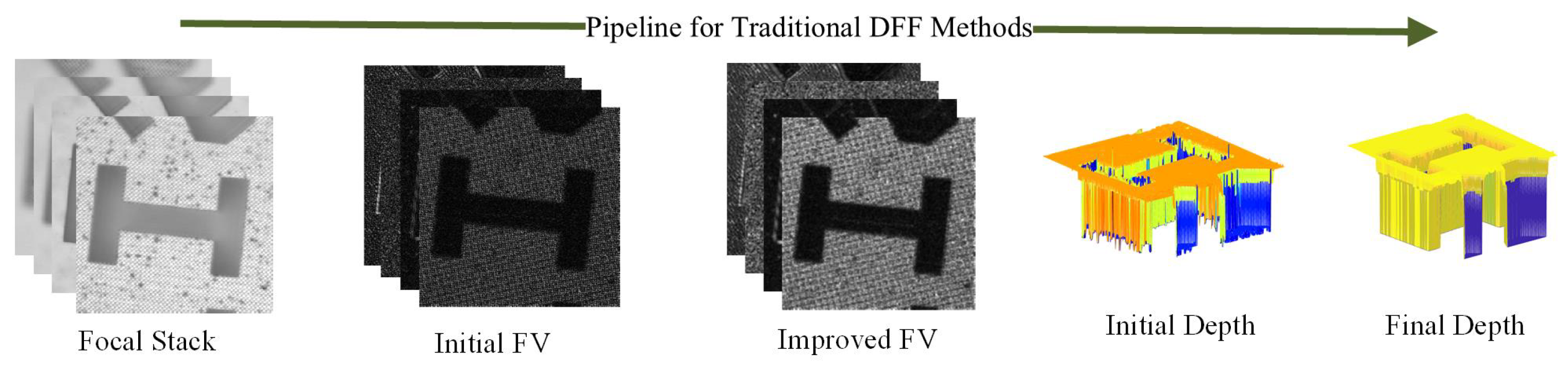
Figure 1.
Steps in traditional depth-from-focus methods.
Figure 1.
Steps in traditional depth-from-focus methods.
Figure 2.
Pipeline for deep learning-based depth from focus methods.
Figure 2.
Pipeline for deep learning-based depth from focus methods.
Figure 3.
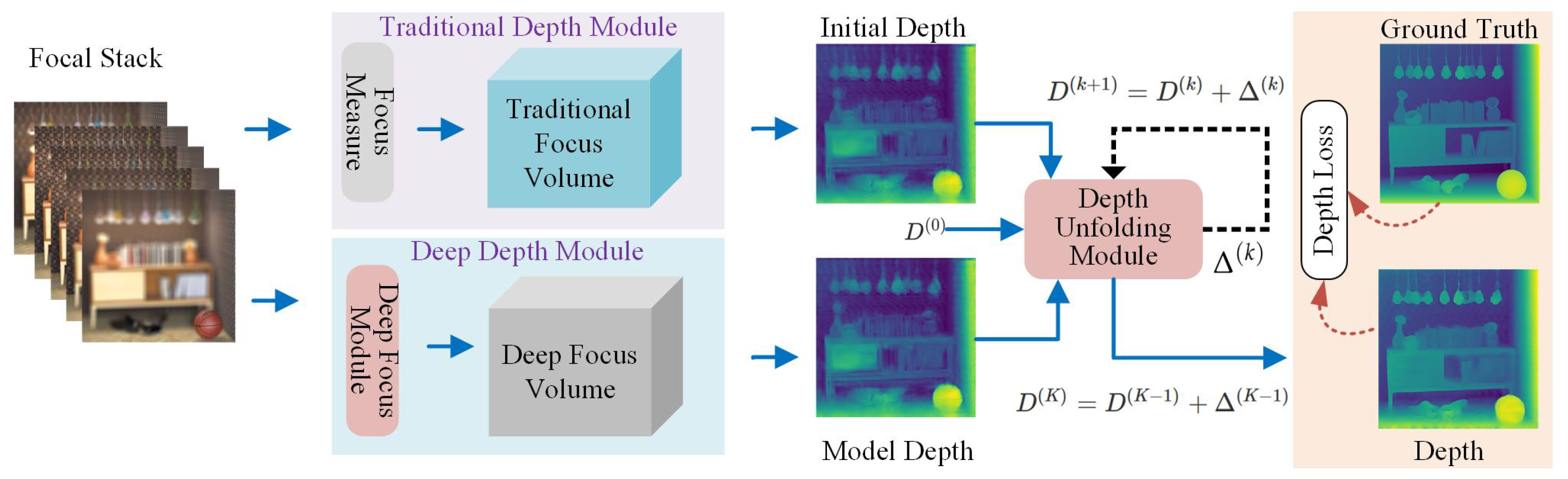
Overview of the proposed framework: The proposed network takes a focal stack . The deep depth and traditional depth modules compute deep and traditional depths, which are provided to the depth unfolding module that yields the final depth .
Figure 3.
Overview of the proposed framework: The proposed network takes a focal stack . The deep depth and traditional depth modules compute deep and traditional depths, which are provided to the depth unfolding module that yields the final depth .
Figure 4.
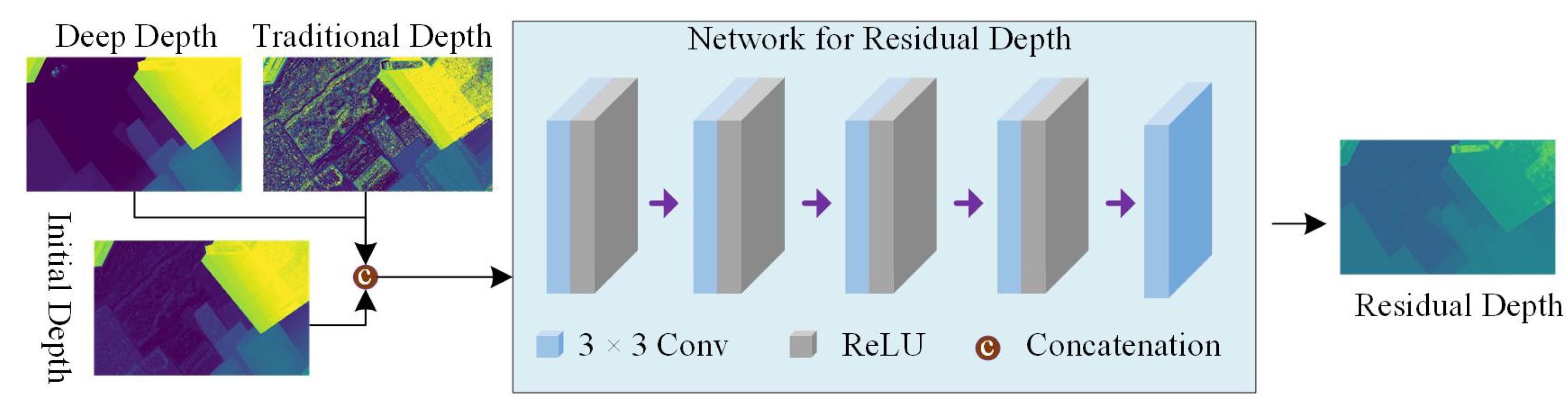
Depth unfolding module: It takes deep depth and traditional depth , along with the initial depth , and computes depth corrections (residual depth), . The final refined depth is obtained by adding depth corrections at each iteration.
Figure 4.
Depth unfolding module: It takes deep depth and traditional depth , along with the initial depth , and computes depth corrections (residual depth), . The final refined depth is obtained by adding depth corrections at each iteration.
Figure 5.
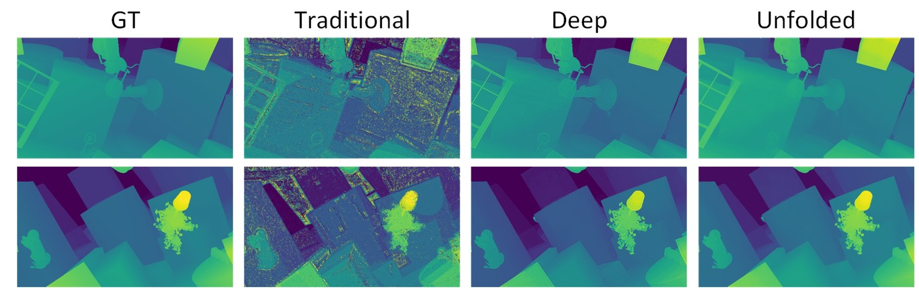
Visualization of output maps at different stages. The first column shows the ground truth, the second shows the deep output map, the third shows the traditional output map, and the last shows the unfolded map. Rows correspond to outputs from different samples.
Figure 5.
Visualization of output maps at different stages. The first column shows the ground truth, the second shows the deep output map, the third shows the traditional output map, and the last shows the unfolded map. Rows correspond to outputs from different samples.
Figure 6.
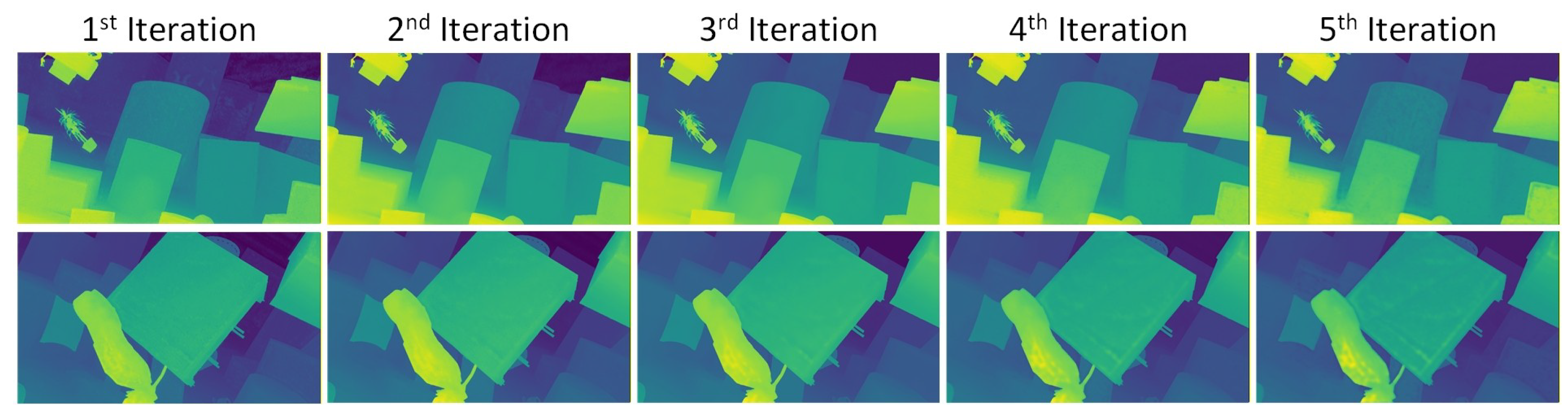
Qualitative results on the FT dataset after different numbers of iterations. Columns represent different iteration counts, while rows correspond to outputs from different samples.
Figure 6.
Qualitative results on the FT dataset after different numbers of iterations. Columns represent different iteration counts, while rows correspond to outputs from different samples.
Figure 7.
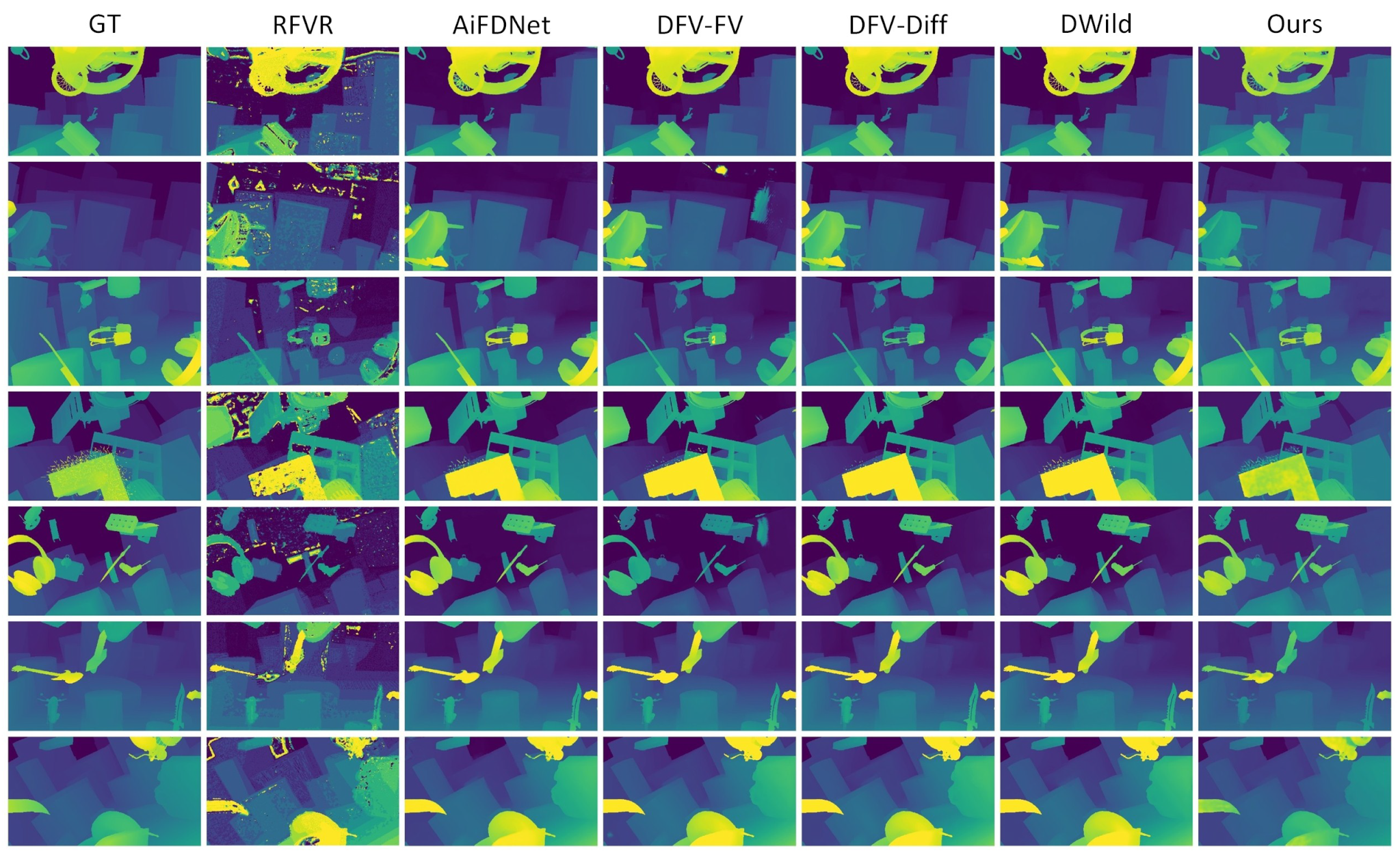
Qualitative comparison on the FT dataset. The columns show the GT output maps followed by the results from RFVR, AiFDNet, DFV-FV, DFV-Diff, DWild, and our method. The rows correspond to results obtained from focal stacks {4, 15, 24, 34, 54, 64, 75}.
Figure 7.
Qualitative comparison on the FT dataset. The columns show the GT output maps followed by the results from RFVR, AiFDNet, DFV-FV, DFV-Diff, DWild, and our method. The rows correspond to results obtained from focal stacks {4, 15, 24, 34, 54, 64, 75}.
Figure 8.
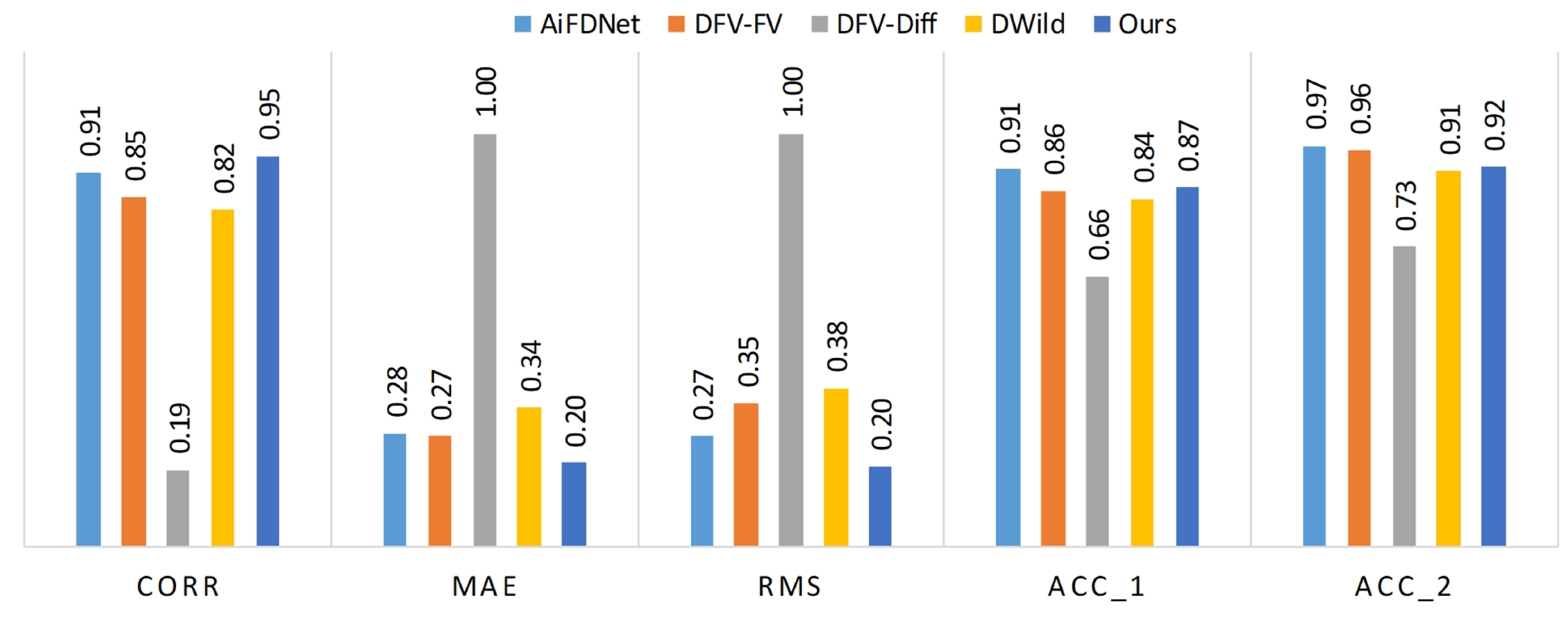
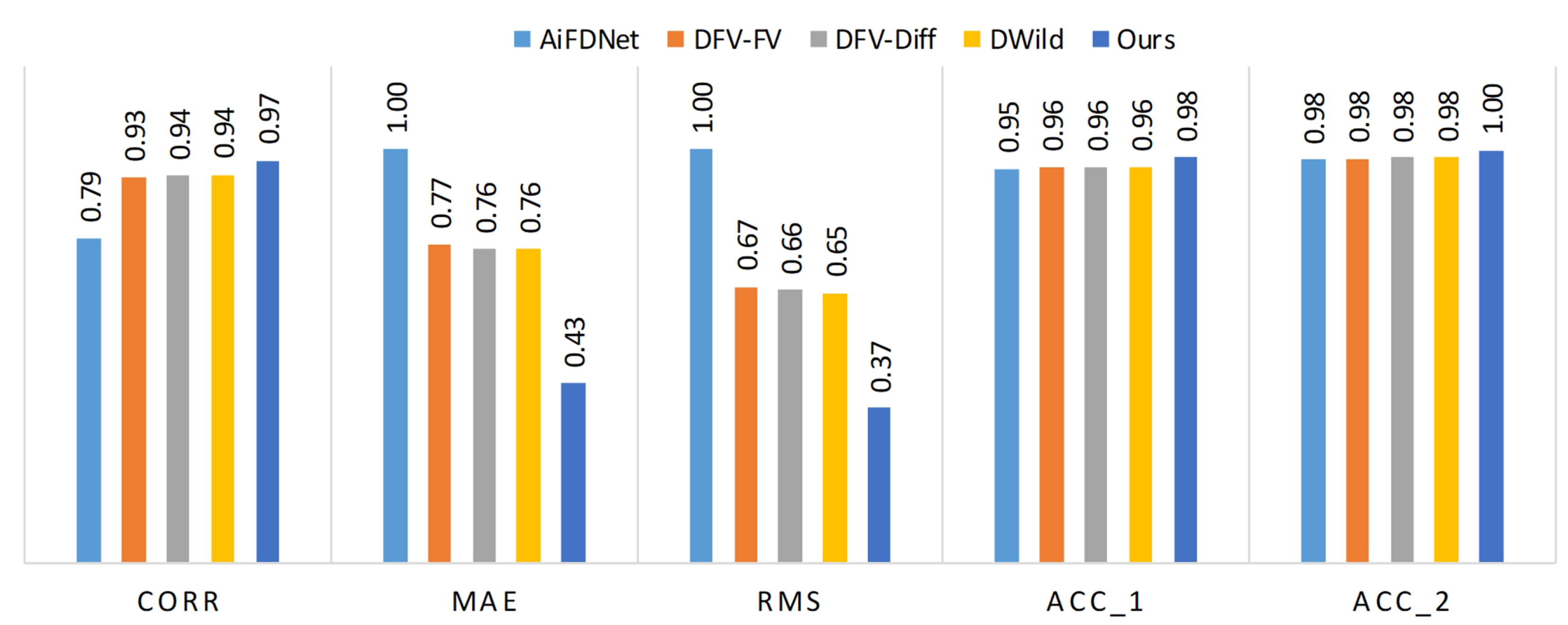
Quantitative comparison for focal stack number 30 from the FT dataset. The values for all measures are normalized within the range . The metrics Corr, MAE, RMS, Acc_1, and Acc_2 are shown for AiFDNet, DFV-FV, DFV-Diff, DWild, and our method.
Figure 8.
Quantitative comparison for focal stack number 30 from the FT dataset. The values for all measures are normalized within the range . The metrics Corr, MAE, RMS, Acc_1, and Acc_2 are shown for AiFDNet, DFV-FV, DFV-Diff, DWild, and our method.
Figure 9.
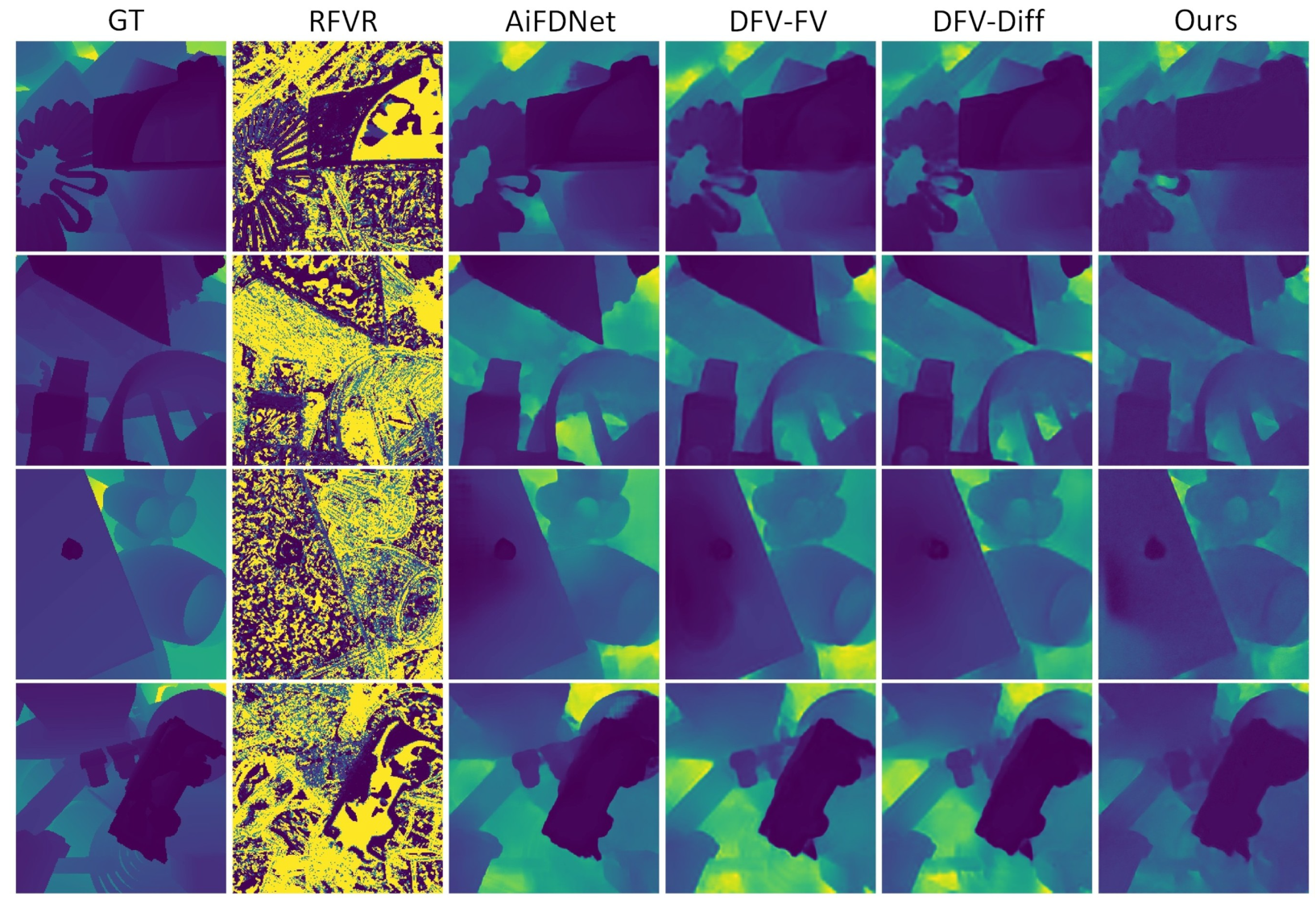
Comparison on the FOD dataset. The first column shows the GT depth maps, and the remaining columns show depth maps from RFVR, AiFDNet, DFV-FV, DFV-Diff, and our method, respectively. The rows correspond to the results obtained from focal stacks {7, 8, 13, 35}.
Figure 9.
Comparison on the FOD dataset. The first column shows the GT depth maps, and the remaining columns show depth maps from RFVR, AiFDNet, DFV-FV, DFV-Diff, and our method, respectively. The rows correspond to the results obtained from focal stacks {7, 8, 13, 35}.
Figure 10.
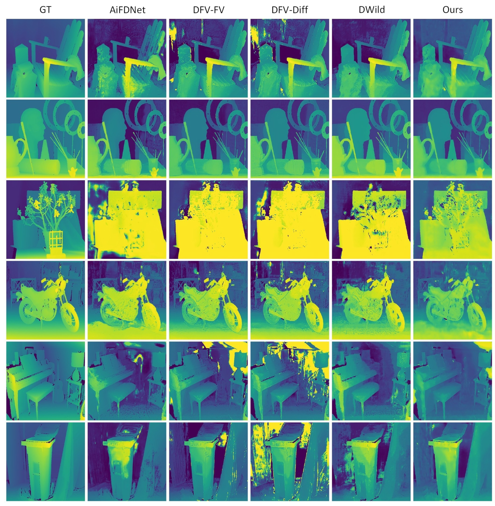
Qualitative comparison on the MB dataset. The columns show the GT output maps followed by the results from AiFDNet, DFV-FV, DFV-Diff, DWild, and our method. The rows correspond to results obtained from focal stacks {0, 1, 2, 3, 6, 11}.
Figure 10.
Qualitative comparison on the MB dataset. The columns show the GT output maps followed by the results from AiFDNet, DFV-FV, DFV-Diff, DWild, and our method. The rows correspond to results obtained from focal stacks {0, 1, 2, 3, 6, 11}.
Figure 11.
Quantitative comparison for focal stack number 11 from the MB dataset. The values for all measures are normalized within the range . The metrics CORR, MAE, RMS, Acc_1, and Acc_2 are shown for AiFDNet, DFV-FV, DFV-Diff, DWild, and our methods.
Figure 11.
Quantitative comparison for focal stack number 11 from the MB dataset. The values for all measures are normalized within the range . The metrics CORR, MAE, RMS, Acc_1, and Acc_2 are shown for AiFDNet, DFV-FV, DFV-Diff, DWild, and our methods.
Figure 12.
Qualitative comparison of a failure case from focal stack 14 from the MB dataset. The GT and results from AiFDNet, DFV-FV, DFV-Diff, and DWild are compared with our method. While none of the models fully capture the correct distance of objects from the viewpoint, our approach remains comparatively closer to the GT.
Figure 12.
Qualitative comparison of a failure case from focal stack 14 from the MB dataset. The GT and results from AiFDNet, DFV-FV, DFV-Diff, and DWild are compared with our method. While none of the models fully capture the correct distance of objects from the viewpoint, our approach remains comparatively closer to the GT.
Table 1.
Quantitative results for focal stack sample 1 from the FT dataset. Rows represent iterations, while columns denote metric evaluations at the corresponding iteration. ↑ indicates that higher values represent better performance, while ↓ indicates that lower values are better. The bold values indicate the best results.
Table 1.
Quantitative results for focal stack sample 1 from the FT dataset. Rows represent iterations, while columns denote metric evaluations at the corresponding iteration. ↑ indicates that higher values represent better performance, while ↓ indicates that lower values are better. The bold values indicate the best results.
| Iteration | MAE ↓ | RMS ↓ | AbsRel ↓ | Acc_1 ↑ | Acc_2 ↑ | Acc_3 ↑ |
|---|
| 1st | 10.28 | 11.93 | 0.47 | 10.34 | 91.91 | 93.88 |
| 2nd | 5.18 | 6.20 | 0.23 | 92.01 | 93.74 | 95.04 |
| 3rd | 0.74 | 1.82 | 0.04 | 98.53 | 99.43 | 99.66 |
| 4th | 6.82 | 8.39 | 0.22 | 74.16 | 97.44 | 98.18 |
| 5th | 18.92 | 24.02 | 0.53 | 11.03 | 59.01 | 98.50 |
Table 2.
Quantitative results for the whole test FT dataset. Rows represent the iteration, while columns denote the metric evaluation at the respective iteration. ↑ indicates that the higher values provide better performance, while ↓ indicates that the lower value is better. The bold values indicate the best results.
Table 2.
Quantitative results for the whole test FT dataset. Rows represent the iteration, while columns denote the metric evaluation at the respective iteration. ↑ indicates that the higher values provide better performance, while ↓ indicates that the lower value is better. The bold values indicate the best results.
| Iteration | MAE ↓ | RMS ↓ | AbsRel ↓ | Acc_1 ↑ | Acc_2 ↑ | Acc_3 ↑ |
|---|
| 1st | 17.05 | 21.85 | 0.63 | 4.04 | 82.89 | 88.28 |
| 2nd | 9.92 | 13.76 | 0.36 | 81.79 | 88.49 | 92.52 |
| 3rd | 3.16 | 6.88 | 0.15 | 95.23 | 98.23 | 99.38 |
| 4th | 10.85 | 15.68 | 0.37 | 68.35 | 96.63 | 97.88 |
| 5th | 32.66 | 46.02 | 0.81 | 15.11 | 52.76 | 92.48 |
Table 3.
Overall quantitative comparison for FT dataset. Rows represent the method employed, while columns denote the metric evaluation of the respective method. ↑ indicates that the higher values provide better performance while ↓ indicates that the lower value is better. The bold values indicate the best results.
Table 3.
Overall quantitative comparison for FT dataset. Rows represent the method employed, while columns denote the metric evaluation of the respective method. ↑ indicates that the higher values provide better performance while ↓ indicates that the lower value is better. The bold values indicate the best results.
| Method | Corr ↑ | MAE ↓ | RMS ↓ | logRMS ↓ | AbsRel ↓ | SqRel ↓ | Acc_1 ↑ | Acc_2 ↑ | Acc_3 ↑ |
|---|
| RFVR | 0.73 | 11.89 | 23.63 | 0.79 | 1.55 | 82.66 | 72.79 | 80.81 | 84.60 |
| AiFDNet | 0.93 | 6.81 | 13.14 | 0.59 | 0.73 | 11.30 | 85.43 | 87.67 | 88.87 |
| DFV-FV | 0.94 | 6.33 | 12.09 | 0.57 | 0.90 | 27.04 | 85.09 | 87.60 | 89.52 |
| DFV-Diff | 0.97 | 5.51 | 10.65 | 0.53 | 0.62 | 7.48 | 86.18 | 88.09 | 89.93 |
| DWild | 0.97 | 5.54 | 10.44 | 0.53 | 0.61 | 7.24 | 86.35 | 88.21 | 89.84 |
| Ours | 0.98 | 3.16 | 6.87 | 0.14 | 0.15 | 12.19 | 95.23 | 98.23 | 99.38 |
Table 4.
Quantitative comparison for focal stack number 7 from the FOD dataset, for which its corresponding qualitative results are shown in the first row of
Figure 9. The rows represent different methods, while the columns denote metric evaluations for each corresponding method. The symbol ↑ indicates that higher values represent better performance, whereas ↓ indicates that lower values are better. The bold values indicate the best results.
Table 4.
Quantitative comparison for focal stack number 7 from the FOD dataset, for which its corresponding qualitative results are shown in the first row of
Figure 9. The rows represent different methods, while the columns denote metric evaluations for each corresponding method. The symbol ↑ indicates that higher values represent better performance, whereas ↓ indicates that lower values are better. The bold values indicate the best results.
| Method | Corr ↑ | MAE ↓ | MSE ↓ | RMS ↓ | Acc_1 ↑ | Acc_2 ↑ | Acc_3 ↑ |
|---|
| RFVR | 0.245 | 0.517 | 0.515 | 0.718 | 18.98 | 32.15 | 43.20 |
| AiFDNet | 0.885 | 0.054 | 0.018 | 0.135 | 79.06 | 92.72 | 96.85 |
| DFV-FV | 0.891 | 0.062 | 0.016 | 0.128 | 76.69 | 93.93 | 97.46 |
| DFV-Diff | 0.904 | 0.054 | 0.016 | 0.126 | 81.98 | 95.11 | 97.10 |
| Ours | 0.912 | 0.063 | 0.014 | 0.117 | 73.57 | 91.22 | 97.49 |
Table 5.
Overall quantitative comparison for MB real-world dataset. Rows represent the method employed, while columns denote the metric evaluation of the respective method. ↑ indicates that higher values provide better performance, while ↓ indicates that the lower value is better. The bold values indicate the best results.
Table 5.
Overall quantitative comparison for MB real-world dataset. Rows represent the method employed, while columns denote the metric evaluation of the respective method. ↑ indicates that higher values provide better performance, while ↓ indicates that the lower value is better. The bold values indicate the best results.
| Method | Corr ↑ | MAE ↓ | RMS ↓ | logRMS ↓ | AbsRel ↓ | SqRel ↓ | Acc_1 ↑ | Acc_2 ↑ | Acc_3 ↑ |
|---|
| AiFDNet | 0.86 | 5.23 | 8.30 | 0.30 | 0.61 | 19.86 | 85.19 | 92.22 | 95.86 |
| DFV-FV | 0.79 | 5.21 | 9.67 | 0.32 | 0.53 | 14.52 | 85.83 | 91.43 | 94.90 |
| DFV-Diff | 0.68 | 6.49 | 11.63 | 0.38 | 0.82 | 32.53 | 80.84 | 87.30 | 91.58 |
| DWild | 0.87 | 4.71 | 8.29 | 0.31 | 0.46 | 11.06 | 88.18 | 92.78 | 95.50 |
| Ours | 0.88 | 4.49 | 7.72 | 0.32 | 0.48 | 11.75 | 87.15 | 93.06 | 95.87 |
Table 6.
Parameter count and average inference time on FOD dataset for each evaluated method.
Table 6.
Parameter count and average inference time on FOD dataset for each evaluated method.
| Method | Params (M) | Mean Time (s) |
|---|
| AiFDNet [11] | 16.53 | 0.0272 |
| DFV-FV [6] | 19.5 | 0.0169 |
| DFV-Diff [6] | 19.5 | 0.0179 |
| Ours | 19.53 | 0.0260 |
Table 7.
Quantitative comparison of a failure case from focal stack 14 from the MB dataset. The bold values indicate the best results.
Table 7.
Quantitative comparison of a failure case from focal stack 14 from the MB dataset. The bold values indicate the best results.
| Method | Corr ↑ | MAE ↓ | RMS ↓ | AbsRel ↓ | Acc_1 ↑ | Acc_2 ↑ | Acc_3 ↑ |
|---|
| AiFDNet | 0.56 | 15.96 | 24.23 | 0.35 | 55.77 | 72.15 | 91.32 |
| DFV-FV | 0.48 | 16.56 | 24.22 | 0.38 | 56.85 | 69.68 | 89.04 |
| DFV-Diff | 0.33 | 18.20 | 25.50 | 0.49 | 53.67 | 65.61 | 84.97 |
| DWild | 0.47 | 15.04 | 27.24 | 0.24 | 71.62 | 81.07 | 90.53 |
| Ours | 0.61 | 14.73 | 22.25 | 0.31 | 64.17 | 79.79 | 91.89 |