Oscillation Conditions for Third-Order Delay Differential Equations with Neutral-Type Term

Abstract

In this work, we adopted an approach similar to that of Chatzarakis’, by transforming the oscillation analysis of third-order differential equations into an equivalent first-order problem. A key generalization in our study is the extension coefficient $b\left(t\right)$ from the range $0\le b\left(t\right)\le 1$ to $b\left(t\right)\ge 1$. Moreover, we established several oscillation criteria applicable to the canonical and non-canonical cases. Our conclusions complement and extend the oscillation theory for third-order delay differential equations. Several examples are provided to illustrate our results.

1. Introduction

Delays and oscillations are frequently observed in dynamical models and are often formulated by incorporating external sources or nonlinear diffusion mechanisms, which perturb the system’s natural evolutionary path [1,2]. These methods have broad applications in real-world research. For instance, by studying the qualitative behavior of relatively lower-order differential equations (such as third-order ones), researchers can predict solution properties for more complex higher-order partial differential equations. A canonical example from physics is the following Kuramoto–Sivashinsky equation, which describes pattern formation in reaction–diffusion systems and models instabilities in flame front propagation [3,4].

$$u_t+u_{xxxx}+u_{xx}+{\displaystyle \frac{1}{2}}{u}^2=0.$$

(1)

Through a series of transformations, Equation (1) can be converted into the following third-order delay differential equation [5,6]:

$${\left(a\left(t\right){\left(d\left(t\right)y^{\prime }\left(t\right)\right)}^{\prime }\right)}^{\prime }+c\left(t\right)f\left(y\left(h\left(t\right)\right)\right)=0.$$

Consequently, an increasing number of researchers [7,8,9,10,11,12,13,14,15,16,17,18,19,20,21,22,23,24,25,26,27,28,29,30,31,32] have studied the oscillation and asymptotic behavior of various higher-order delay differential equations. Among these researchers, some have studied the following third-order delay differential equations:

$${\left(a\left(t\right){\left(y^{″}\left(t\right)\right)}^{\gamma }\right)}^{\prime }+c\left(t\right)f\left(y\left(h\left(t\right)\right)\right)=0,$$

(2)

Using the comparison principle, Baculícová and Džurina [9,11] established oscillation criteria to determine whether all the solutions to Equation (2) either oscillate or converge to zero. In a similar vein, by employing the Riccati transformation and inequality techniques, Grace et al. [21], Saker et al. [25], and Li et al. [29,30] established criteria for determining whether the solutions to (2) oscillate or approach zero.

Following this line of research, a number of researchers have focused on the following third-order delay differential equations with a neutral term:

$${\left(a\left(t\right){\left[{(y\left(t\right)+b\left(t\right)y\left(g\left(t\right)\right))}^{″}\right]}^{\gamma }\right)}^{\prime }+c\left(t\right)f\left(h\left(t\right)\right)=0.$$

(3)

By applying the comparison principle, Baculíková and Li [8,31] established criteria for the solutions to (3) to either oscillate or tend to zero. Using the Riccati transformation and inequality techniques, Baculĺková et al. [10,27,28] established criteria to verify that the solution to (3) either oscillates or approaches zero. By applying the iterative method, Jadlovská and Li [32] studied the oscillations of Equation (3).

These researchers generally established criteria for the oscillation and asymptotic behavior of solutions under the conditions that $a\left(t\right)$ satisfies ${\int }_{t_0}^{\infty }{a}^{-\gamma }\left(t\right)dt=\infty$ and the neutral coefficient $b\left(t\right)$ satisfies $0\le b\left(t\right)<1$ or $0\le b\left(t\right)\le b_0<\infty$. For third-order neutral delay differential equations, when discussing the classification of $y\left(t\right)+b\left(t\right)y\left(g\right(t\left)\right)$, the situation where $y\left(t\right)+b\left(t\right)y\left(g\right(t\left)\right)>0$ and ${(y\left(t\right)+b\left(t\right)y\left(g\left(t\right)\right))}^{\prime }<0$ often arises. Without a more detailed analysis, one can only derive the oscillation and asymptotic behavior of the solutions to such equations.

Thus, Chatzarakis et al. [33] directly provided the oscillation criteria for the following class of third-order nonlinear neutral delay differential equations:

$${(y\left(t\right)+b\left(t\right)y\left(g\left(t\right)\right))}^{‴}+c\left(t\right)y^{\eta }\left(h\left(t\right)\right)=0.$$

(4)

When $b\left(t\right)\ge 1$ and $b\left(t\right)\not\equiv 1$, Chatzarakis et al. [33] transformed the oscillation problem of Equation (4) into studying first-order delay differential equations, thereby establishing the oscillation criteria for Equation (4).

Inspired by the above research, in this paper, we considered the oscillations of the following third-order neutral delay differential equation:

$${\left(a\left(t\right){\chi }^{″}\left(t\right)\right)}^{\prime }+c\left(t\right)y^{\eta }\left(h\left(t\right)\right)=0,$$

(5)

where $\chi \left(t\right)=y\left(t\right)+b\left(t\right)y\left(g\right(t\left)\right)$, $t_0\in \mathbb{R}$, $a\left(t\right)\in C^1([t_0,\infty ),(0,\infty ))$, $b\left(t\right)\in C^3([t_0,\infty ),(0,\infty ))$, $c\left(t\right)\in C([t_0,\infty ),(0,\infty ))$, $g\left(t\right)\in C^3([t_0,\infty ),\mathbb{R})$, $h\left(t\right)\in C([t_0,\infty ),\mathbb{R})$, $g\left(t\right)\le t,h\left(t\right)\le t$, $\underset{t\to \infty }{lim}g\left(t\right)=\underset{t\to \infty }{lim}h\left(t\right)=\infty$, and $\eta$ is the quotient of odd positive integers. And the following assumptions are satisfied:

(A1)

$a\left(t\right)>0,a^{\prime }\left(t\right)\ge 0$;

(A2)

$b\left(t\right)\ge 1$, $b\left(t\right)\not\equiv 1$;

(A3)

$g^{\prime }\left(t\right)\ge g_0>0$, $g^{-1}\left(t\right)$ is the inverse function of $g\left(t\right)$, $h^{\prime }\left(t\right)>0$;

(A4)

There exists a function $\sigma \in C^1([t_0,\infty ),\infty )$ such that $h\left(t\right)\le \sigma \left(t\right)\le g\left(t\right)$ for $t\ge t_0$.

If

$${\int }_{t_0}^{\infty }{\displaystyle \frac{1}{a\left(t\right)}}dt=\infty ,$$

(6)

then we say that Equation (5) satisfies the canonical case.

If

$${\int }_{t_0}^{\infty }{\displaystyle \frac{1}{a\left(t\right)}}dt<\infty ,$$

(7)

then we say that Equation (5) satisfies the non-canonical case.

We only considered the nontrivial solution of (5) that satisfies $sup\left\{\right|x\left(t\right)|:t\ge T\}>0$ for all $T\ge t_0$.

A nontrivial solution of (5) is oscillatory if it has an arbitrarily large zero point on the interval $I=[t_0,\infty )$. Otherwise, it is non-oscillatory. Equation (5) is oscillatory if all of its solutions are oscillatory.

In this paper, we adopted a method similar to that of Chatzarakis et al. [33], reducing the oscillation problem of a third-order differential equation to that of a first-order differential equation. Compared with previous research results, we extended the neutral coefficient $b\left(t\right)$ from the the case of $0\le b\left(t\right)\le 1$ to the case of $b\left(t\right)\ge 1$ and established oscillation criteria for both the canonical and non-canonical cases. Our conclusions complement and refine the oscillation theory for third-order delay differential equations.

For convenience, we introduce the following notation:

$$\varpi \left(t\right):={\displaystyle \frac{1}{b\left(g^{-1}\left(t\right)\right)}}\left(1-{\displaystyle \frac{{\left(g^{-1}\left(g^{-1}\left(t\right)\right)\right)}^{\frac{2}{l}}}{{\left(g^{-1}\left(t\right)\right)}^{\frac{2}{l}}b\left(g^{-1}\left(g^{-1}\left(t\right)\right)\right)}}\right),$$

$${\varpi }_1\left(t\right):={\displaystyle \frac{1}{b\left(g^{-1}\left(t\right)\right)}}\left(1-{\displaystyle \frac{{\left(g^{-1}\left(g^{-1}\left(t\right)\right)\right)}^{\frac{1}{l}}}{{\left(g^{-1}\left(t\right)\right)}^{\frac{1}{l}}b\left(g^{-1}\left(g^{-1}\left(t\right)\right)\right)}}\right),$$

$$\varrho \left(t\right):={\displaystyle \frac{1}{b\left(g^{-1}\left(t\right)\right)}}\left(1-{\displaystyle \frac{1}{b\left(g^{-1}\left(g^{-1}\left(t\right)\right)\right)}}\right).$$

2. Main Results

First, we investigated the oscillatory behavior of (5) in the canonical case. To analyze the oscillation properties of Equation (5), the following lemmas are required.

Lemma 1

([34]). If a function f satisfies $f^{\left(i\right)}>0$ for $i=1,2,\dots ,k$ and $f^{(k+1)}\le 0$, then for any $l\in (0,1)$, ${\displaystyle \frac{f\left(t\right)}{f^{\prime }\left(t\right)}}\ge {\displaystyle \frac{lt}{k}}$.

Lemma 2.

Let $y\left(t\right)$ be an eventually positive solution of Equation (5). If (A1) and (6) hold, then according to Equation (5), there exists $t_1\ge t_0$ such that, for $t\ge t_1$, one of the following cases holds:

(I)

$\chi \left(t\right)>0$, ${\chi }^{\prime }\left(t\right)>0$, ${\chi }^{″}\left(t\right)>0$, ${\chi }^{‴}\left(t\right)<0$;

(II)

$\chi \left(t\right)>0$, ${\chi }^{\prime }\left(t\right)<0$, ${\chi }^{″}\left(t\right)>0$, ${\chi }^{‴}\left(t\right)<0$.

Proof. 

Suppose $y\left(t\right)$ is an eventually positive solution of Equation (5). Then, there exists a sufficiently large $t_1\ge t_0$ such that, for $t\ge t_1$,

$$y\left(t\right)>0,y\left(g\right(t\left)\right)>0,y\left(h\right(t\left)\right)>0.$$

Because $b\left(t\right)\ge 0$, we have $\chi \left(t\right)>0$ for $t\ge t_1$. From Equation (5), it follows that

$${\left(a\left(t\right){\chi }^{″}\left(t\right)\right)}^{\prime }=-c\left(t\right)y^{\eta }\left(h\left(t\right)\right)<0.$$

(8)

Thus, $a\left(t\right){\chi }^{″}\left(t\right)$ is non-increasing and of one sign. Since $a\left(t\right)>0$, then ${\chi }^{″}\left(t\right)$ is also of one sign and we have two possibilities, i.e., either ${\chi }^{″}\left(t\right)>0$ or ${\chi }^{″}\left(t\right)<0$ for $t\ge t_1$. Below, we assert that ${\chi }^{″}\left(t\right)>0$ holds for $t\ge t_1$.

Suppose that ${\chi }^{″}\left(t\right)<0$ for $t\ge t_1$, meaning that $a\left(t\right){\chi }^{″}\left(t\right)<0$. Since $a\left(t\right){\chi }^{″}\left(t\right)$ is non-increasing, there exists a positive constant m such that

$$a\left(t\right){\chi }^{″}\left(t\right)\le -m<0.$$

By integrating this from $t_1$ to t, we have

$${\chi }^{\prime }\left(t\right)\le {\chi }^{\prime }\left(t_1\right)-m{\int }_{t_1}^t{a}^{-1}\left(s\right)ds.$$

By letting $t\to \infty$ and using (6), we get ${\chi }^{\prime }\left(t\right)\to -\infty$. Since ${\chi }^{″}\left(t\right)<0$, there exists a positive constant $m_1$ such that

$${\chi }^{\prime }\left(t\right)<-m_1.$$

By integrating this from $t_1$ to t, we obtain

$$\chi \left(t\right)\le \chi \left(t_1\right)-m_1(t-t_1).$$

By letting $t\to \infty$, we get $\chi \left(t\right)<0$, which contradicts $\chi \left(t\right)>0$. Therefore, ${\chi }^{″}\left(t\right)>0$.

Since ${\chi }^{″}\left(t\right)>0$ and $a^{\prime }\left(t\right)$ and $a\left(t\right)$ are positive, it follows from the inequality (8) that ${\chi }^{‴}\left(t\right)<0$. Thus, since ${\chi }^{″}\left(t\right)>0$, ${\chi }^{\prime }\left(t\right)$ is increasing. Therefore, ${\chi }^{\prime }\left(t\right)$ is of one sign, i.e., either ${\chi }^{\prime }\left(t\right)>0$ or ${\chi }^{\prime }\left(t\right)<0$ for $t\ge t_1$. This corresponds to cases (I) and (II). □

Theorem 1.

Suppose (A1), (A2), (A3), (A4), and (6) hold. If there exist constants $l\in (0,1)$ such that the first-order delay differential equations

$$w^{\prime }\left(t\right)+c\left(t\right){\displaystyle \frac{l^{\eta }}{{\left(2a\left(g^{-1}\left(h\left(t\right)\right)\right)\right)}^{\eta }}}{\varpi }^{\eta }\left(h\left(t\right)\right){\left(g^{-1}\left(h\left(t\right)\right)\right)}^{2\eta }{\left(w\left(g^{-1}\left(h\left(t\right)\right)\right)\right)}^{\eta }=0$$

(9)

and

$$Y^{\prime }\left(t\right)+{\displaystyle \frac{c\left(t\right)}{2^{\eta }{a}^{\eta }\left(g^{-1}\left(\sigma \left(t\right)\right)\right)}}{\varrho }^{\eta }\left(h\left(t\right)\right){(g^{-1}\left(\sigma \left(t\right)\right)-g^{-1}\left(h\left(t\right)\right))}^{2\eta }{Y}^{\eta }\left(g^{-1}\left(\sigma \left(t\right)\right)\right)=0$$

(10)

are oscillatory, then Equation (5) is oscillatory.

Proof. 

Suppose, for the sake of contradiction, that Equation (5) is non-oscillatory. Without the loss of generality, assume y is an eventually positive solution to Equation (5). That is, there exists a sufficiently large $t_1$ such that $y\left(t\right)>0$, $y\left(g\right(t\left)\right)>0$, and $y\left(h\right(t\left)\right)>0$ for $t\ge t_1$. According to the assumptions and Lemma 2, we only need to consider the two cases stated in Lemma 2.

First, consider case (I) in Lemma 2. From the definition of $\chi \left(t\right)$, we get

$$\begin{array}{cc}\hfill y\left(t\right)& ={\displaystyle \frac{\chi \left(g^{-1}\left(t\right)\right)}{b\left(g^{-1}\left(t\right)\right)}}-{\displaystyle \frac{\chi \left(g^{-1}\left(g^{-1}\left(t\right)\right)\right)-y\left(g^{-1}\left(g^{-1}\left(t\right)\right)\right)}{b\left(g^{-1}\left(t\right)\right)b\left(g^{-1}\left(g^{-1}\left(t\right)\right)\right)}}\hfill \\ \hfill & \ge {\displaystyle \frac{\chi \left(g^{-1}\left(t\right)\right)}{b\left(g^{-1}\left(t\right)\right)}}-{\displaystyle \frac{\chi \left(g^{-1}\left(g^{-1}\left(t\right)\right)\right)}{b\left(g^{-1}\left(t\right)\right)b\left(g^{-1}\left(g^{-1}\left(t\right)\right)\right)}}.\hfill \end{array}$$

(11)

For $k=2$, according to Lemma 1, for any constant $l_1\in (0,1)$, we have

$${\displaystyle \frac{\chi \left(t\right)}{{\chi }^{\prime }\left(t\right)}}\ge {\displaystyle \frac{l_{1}t}{2}}.$$

(12)

This implies that the following inequality holds:

$${\left({\displaystyle \frac{\chi \left(t\right)}{t^{\frac{2}{l_1}}}}\right)}^{\prime }={\displaystyle \frac{t{\chi }^{\prime }\left(t\right)-\frac{2}{l_1}\chi \left(t\right)}{t^{\frac{2}{l_1}+1}}}\le 0.$$

Therefore, ${\displaystyle \frac{\chi \left(t\right)}{t^{\frac{2}{l_1}}}}$ is non-increasing on the interval $[t_1,\infty )$. From $g\left(t\right)\le t$ and the monotonicities of $g\left(t\right)$ and ${\displaystyle \frac{\chi \left(t\right)}{t^{\frac{2}{l_1}}}}$, we obtain

$$\chi \left(g^{-1}\left(g^{-1}\left(t\right)\right)\right)\le {\displaystyle \frac{{\left(g^{-1}\left(g^{-1}\left(t\right)\right)\right)}^{\frac{2}{l_1}}}{{\left(g^{-1}\left(t\right)\right)}^{\frac{2}{l_1}}}}\chi \left(g^{-1}\left(t\right)\right).$$

Hence, we have

$$y\left(t\right)\ge \varpi \left(t\right)\chi \left(g^{-1}\left(t\right)\right).$$

Thus,

$$y\left(h\left(t\right)\right)\ge \varpi \left(h\left(t\right)\right)\chi \left(g^{-1}\left(h\left(t\right)\right)\right).$$

(13)

By substituting inequality (13) into (5), we derive

$${\left(a\left(t\right){\chi }^{″}\left(t\right)\right)}^{\prime }+c\left(t\right){\varpi }^{\eta }\left(h\left(t\right)\right){\chi }^{\eta }\left(g^{-1}\left(h\left(t\right)\right)\right)\le 0.$$

(14)

By substituting inequality (12) into Equation (14), we obtain

$${\left(a\left(t\right){\chi }^{″}\left(t\right)\right)}^{\prime }+c\left(t\right){\displaystyle \frac{l_1^{\eta }}{2^{\eta }}}{\varpi }^{\eta }\left(h\left(t\right)\right){\left(g^{-1}\left(h\left(t\right)\right)\right)}^{\eta }{\left({\chi }^{\prime }\left(g^{-1}\left(h\left(t\right)\right)\right)\right)}^{\eta }\le 0.$$

(15)

Let $u\left(t\right):={\chi }^{\prime }\left(t\right)$. Then, $u\left(t\right)>0$, $u^{\prime }\left(t\right)>0$, and $u^{″}\left(t\right)<0$. Therefore, for $k=1$, according to Lemma 1, for all $l_2\in (0,1)$, we have

$${\displaystyle \frac{u\left(t\right)}{u^{\prime }\left(t\right)}}\ge l_{2}t,$$

and so,

$$u\left(g^{-1}\left(h\left(t\right)\right)\right)\ge l_2{g}^{-1}\left(h\left(t\right)\right)u^{\prime }\left(g^{-1}\left(h\left(t\right)\right)\right).$$

(16)

By substituting $u\left(t\right)={\chi }^{\prime }\left(t\right)$ and (16) into (15), we obtain

$${\left(a\left(t\right)u^{\prime }\left(t\right)\right)}^{\prime }+c\left(t\right){\displaystyle \frac{l^{\eta }}{2^{\eta }}}{\varpi }^{\eta }\left(h\left(t\right)\right){\left(g^{-1}\left(h\left(t\right)\right)\right)}^{2\eta }{\left(u^{\prime }\left(g^{-1}\left(h\left(t\right)\right)\right)\right)}^{\eta }\le 0.$$

(17)

By letting $w\left(t\right):=a\left(t\right)u^{\prime }\left(t\right)$, due to the positivity of $a\left(t\right)$ and $u^{\prime }\left(t\right)$, we get $w\left(t\right)>0$. By substituting w into Equation (17), we can find that $w\left(t\right)$ is an eventually positive solution of the following first-order delay differential equation:

$$w^{\prime }\left(t\right)+c\left(t\right){\displaystyle \frac{l^{\eta }}{{\left(2a\left(g^{-1}\left(h\left(t\right)\right)\right)\right)}^{\eta }}}{\varpi }^{\eta }\left(h\left(t\right)\right){\left(g^{-1}\left(h\left(t\right)\right)\right)}^{2\eta }{\left(w\left(g^{-1}\left(h\left(t\right)\right)\right)\right)}^{\eta }\le 0.$$

Therefore, according to [35] (Theorem 1), for any $l\in (0,1)$, Equation (9) has an eventually positive solution. This contradicts its oscillatory nature.

For case (II) in Lemma 2, since $g\left(t\right)\le t$ and based on the monotonicities of $\chi$ and $g^{-1}\left(t\right)$, we obtain

$$\chi \left(g^{-1}\left(t\right)\right)\ge \chi \left(g^{-1}\left(g^{-1}\left(t\right)\right)\right).$$

From (11), it follows that

$$y\left(t\right)\ge \varrho \left(t\right)\chi \left(g^{-1}\left(t\right)\right).$$

Thus,

$$y\left(h\left(t\right)\right)\ge \varrho \left(h\left(t\right)\right)\chi \left(g^{-1}\left(h\left(t\right)\right)\right).$$

(18)

Substituting this into Equation (5) yields

$${\left(a\left(t\right){\chi }^{″}\left(t\right)\right)}^{\prime }+c\left(t\right){\varrho }^{\eta }\left(h\left(t\right)\right){\chi }^{\eta }\left(g^{-1}\left(h\left(t\right)\right)\right)\le 0.$$

(19)

According to $\chi \left(t\right)>0$, ${\chi }^{\prime }\left(t\right)<0$, ${\chi }^{″}\left(t\right)>0$, and ${\chi }^{‴}\left(t\right)<0$, for $\gamma \ge \theta \ge t_2$, we have

$$\chi \left(\theta \right)\ge {\displaystyle \frac{{(\gamma -\theta )}^2}{2}}{\chi }^{″}\left(\gamma \right).$$

(20)

Since $h\left(t\right)\le \sigma \left(t\right)$ and $g^{-1}\left(t\right)$ is strictly increasing, we get $g^{-1}\left(h\left(t\right)\right)\le g^{-1}\left(\sigma \left(t\right)\right)$. Substituting $\theta =g^{-1}\left(h\left(t\right)\right)$ and $\gamma =g^{-1}\left(\sigma \left(t\right)\right)$ into inequality (20) gives

$$\chi \left(g^{-1}\left(h\left(t\right)\right)\right)\ge {\displaystyle \frac{{(g^{-1}\left(\sigma \left(t\right)\right)-g^{-1}\left(h\left(t\right)\right))}^2}{2}}{\chi }^{″}\left(g^{-1}\left(\sigma \left(t\right)\right)\right).$$

Using this in inequality (19) leads to

$${\left(a\left(t\right){\chi }^{″}\left(t\right)\right)}^{\prime }+{\displaystyle \frac{c\left(t\right)}{2^{\eta }}}{\varrho }^{\eta }\left(h\left(t\right)\right)·{(g^{-1}\left(\sigma \left(t\right)\right)-g^{-1}\left(h\left(t\right)\right))}^{2\eta }{\chi }^{″}\left(g^{-1}\left(\sigma \left(t\right)\right)\right)\le 0.$$

By letting $Y\left(t\right):=a\left(t\right){\chi }^{″}\left(t\right)$, due to the positivity of $a\left(t\right)$ and ${\chi }^{″}\left(t\right)$, we get $Y\left(t\right)>0$. Then, $Y\left(t\right)$ is an eventually positive solution to the following first-order delay differential inequality:

$$Y^{\prime }\left(t\right)+{\displaystyle \frac{c\left(t\right)}{2^{\eta }{a}^{\eta }\left(g^{-1}\left(\sigma \left(t\right)\right)\right)}}{\varrho }^{\eta }\left(h\left(t\right)\right)·{(g^{-1}\left(\sigma \left(t\right)\right)-g^{-1}\left(h\left(t\right)\right))}^{2\eta }{Y}^{\eta }\left(g^{-1}\left(\sigma \left(t\right)\right)\right)\le 0.$$

Therefore, by [35] (Theorem 1), Equation (9) also admits an eventually positive solution. This contradicts its oscillatory nature. □

Corollary 1.

Assume that (A1), (A2), (A3), (A4), and (6) hold and $\eta =1$. If there exists a constant $l\in (0,1)$ such that the two inequalities

$$\underset{t\to \infty }{lim\; inf}{\int }_{g^{-1}\left(h\left(t\right)\right)}^t{\displaystyle \frac{c\left(s\right)}{a\left(g^{-1}\left(h\left(s\right)\right)\right)}}\varpi \left(h\left(s\right)\right){\left(g^{-1}\left(h\left(s\right)\right)\right)}^{2}ds>{\displaystyle \frac{2}{le}},$$

(21)

$$\underset{t\to \infty }{lim\; inf}{\int }_{g^{-1}\left(\sigma \left(t\right)\right)}^t{\displaystyle \frac{c\left(s\right)}{a\left(g^{-1}\left(\sigma \left(s\right)\right)\right)}}\varrho \left(h\left(s\right)\right)·{\left(g^{-1}\left(\sigma \left(s\right)\right)-g^{-1}\left(h\left(s\right)\right)\right)}^{2}ds>{\displaystyle \frac{2}{e}},$$

(22)

hold, then Equation (5) is oscillatory.

Proof. 

According to [36], if

$$\underset{t\to \infty }{lim\; inf}{\int }_{\tau \left(t\right)}^{t}R\left(s\right)ds>{\displaystyle \frac{1}{e}},$$

then the first-order delay differential equation

$$y^{\prime }\left(t\right)+R\left(t\right)y\left(\tau \left(t\right)\right)=0$$

is oscillatory, where $R,\tau \in C([t_0,\infty ),\mathbb{R})$, $R\left(t\right)\ge 0$, $\tau \left(t\right)\le t$, and $\underset{t\to \infty }{lim}\tau \left(t\right)=\infty$. Therefore, inequalities (21) and (22) imply that Equations (9) and (10) are oscillatory. Consequently, by Theorem 1, Equation (5) is oscillatory. □

Corollary 2.

Assume that (A1), (A2), (A3), (A4), and (6) hold with $\eta <1$. If the two inequalities

$${\int }_{t_0}^{\infty }{\displaystyle \frac{c\left(t\right)}{a^{\eta }\left(g^{-1}\left(h\left(t\right)\right)\right)}}{\varpi }^{\eta }\left(h\left(t\right)\right){\left(g^{-1}\left(h\left(t\right)\right)\right)}^{2\eta }dt=\infty ,$$

(23)

$${\int }_{t_0}^{\infty }{\displaystyle \frac{c\left(t\right)}{a^{\eta }\left(g^{-1}\left(\sigma \left(t\right)\right)\right)}}{\varrho }^{\eta }\left(h\left(t\right)\right)·{\left(g^{-1}\left(\sigma \left(t\right)\right)-g^{-1}\left(h\left(t\right)\right)\right)}^{2\eta }dt=\infty$$

(24)

hold, then Equation (5) is oscillatory.

Proof. 

According to [37] (Theorem 2), inequalities (23) and (24) imply that Equations (9) and (10) are oscillatory. Therefore, by Theorem 1, Equation (5) is oscillatory. □

Example 1.

Consider the following third-order delay differential equation

$${\left(t{\left(y\left(t\right)+ty\left({\displaystyle \frac{t}{2}}\right)\right)}^{″}\right)}^{\prime }+m{t}^{\alpha }{y}^{{\displaystyle \frac{1}{3}}}\left({\displaystyle \frac{t}{4}}\right)=0,t\ge 17,$$

(25)

where $m>0$ and $\alpha >-{\displaystyle \frac{2}{3}}$ are constants. Here, $\eta ={\displaystyle \frac{1}{3}}$, $a\left(t\right)=t$, $b\left(t\right)=t$, $g\left(t\right)={\displaystyle \frac{t}{2}}$, $h\left(t\right)={\displaystyle \frac{t}{4}}$, and $c\left(t\right)=m{t}^{\alpha }$. It is easy to know that Equation (25) satisfies the canonical case because $a\left(t\right)=t$. Under these conditions, the oscillation criteria developed by Chatzarakis et al. [33] become inapplicable due to the specific form of $a\left(t\right)=t$. And according to $\eta ={\displaystyle \frac{1}{3}}$, we used Corollary 2 to verify the oscillatory characteristics of this equation.

By letting $l={\displaystyle \frac{1}{2}}$, we derive the following key relationships: $g^{-1}\left(h\left(t\right)\right)={\displaystyle \frac{t}{2}}$, $\varpi \left(h\left(t\right)\right)={\displaystyle \frac{2(1-16/t)}{t}}$ and $\varrho \left(h\left(t\right)\right)={\displaystyle \frac{2(1-1/t)}{t}}$. Thus, condition (23) becomes

$$\begin{array}{cc}\hfill {\int }_{17}^{\infty }& {\displaystyle \frac{m{t}^{\alpha }}{{(t/2)}^{\frac{1}{3}}}}{\left({\displaystyle \frac{2(1-16/t)}{t}}\right)}^{{\displaystyle \frac{1}{3}}}{\left({\displaystyle \frac{t}{2}}\right)}^{{\displaystyle \frac{2}{3}}}dt\hfill \\ \hfill & ={\int }_{17}^{\infty }{\displaystyle \frac{m{t}^{\alpha -\frac{1}{3}}{(2t-32)}^{\frac{1}{3}}}{2^{\frac{1}{3}}}}dt\hfill \\ \hfill & \ge {\int }_{17}^{\infty }m{t}^{\alpha -{\displaystyle \frac{1}{3}}}dt=m{\displaystyle \frac{1}{\alpha +\frac{2}{3}}}{t}^{\alpha +{\displaystyle \frac{2}{3}}}{|}_{17}^{\infty }=\infty .\hfill \end{array}$$

(26)

There exists $\sigma \left(t\right)={\displaystyle \frac{t}{3}}$ such that (A4) holds. Then, $g^{-1}\left(\sigma \left(t\right)\right)={\displaystyle \frac{2t}{3}}$, and condition (24) becomes

$$\begin{array}{cc}\hfill {\int }_{17}^{\infty }& {\displaystyle \frac{m{t}^{\alpha }}{{(2t/3)}^{\frac{1}{3}}}}{\left({\displaystyle \frac{2(1-1/t)}{t}}\right)}^{{\displaystyle \frac{1}{3}}}{\left({\displaystyle \frac{t}{6}}\right)}^{{\displaystyle \frac{2}{3}}}dt\hfill \\ \hfill & ={\int }_{17}^{\infty }{\displaystyle \frac{m{t}^{\alpha -\frac{1}{3}}{(2t-2)}^{\frac{1}{3}}}{2^{\frac{1}{3}}}}dt\hfill \\ \hfill & \ge {\displaystyle \frac{2^{\frac{2}{3}}}{3^{\frac{1}{3}}}}{\int }_{17}^{\infty }m{t}^{\alpha -{\displaystyle \frac{1}{3}}}dt\hfill \\ \hfill & =m{\displaystyle \frac{1}{\alpha +\frac{2}{3}}}{\displaystyle \frac{2^{\frac{2}{3}}}{3^{\frac{1}{3}}}}{t}^{\alpha +{\displaystyle \frac{2}{3}}}{|}_{17}^{\infty }=\infty .\hfill \end{array}$$

(27)

Therefore, conditions (26) and (27) demonstrate that, when $m>0$, $\alpha >-{\displaystyle \frac{2}{3}}$, inequalities (23) and (24) hold. Consequently, according to Corollary 2, Equation (25) is oscillatory.

Next, we studied the oscillations of Equation (5) in the non-canonical case. Prior to investigating this problem, we need to present the following lemma.

Lemma 3

([38] Lemma 2.3). Let $G\left(u\right)=\alpha u-\beta u^{{\displaystyle \frac{\gamma +1}{\gamma }}}$, where $\beta >0$, α is a constant, and γ is the ratio of two positive odd integers. Then, G attains its maximum at the point $u^{\ast }={\left({\displaystyle \frac{\gamma \alpha }{(\gamma +1)\beta }}\right)}^{\gamma }.$

$$\underset{u\in {\mathbb{R}}^{+}}{max}G=G\left(u^{\ast }\right)={\displaystyle \frac{{\gamma }^{\gamma }}{{(\gamma +1)}^{\gamma +1}}}{\displaystyle \frac{{\alpha }^{\gamma +1}}{{\beta }^{\gamma }}}.$$

Lemma 4.

Let $y\left(t\right)$ be an eventually positive solution to Equation (5). If (A1) and (7) hold, then according to Equation (5), there exists $t_1\ge t_0$ such that, for $t\ge t_1$, one of the following cases holds:

(I)

$\chi \left(t\right)>0$, ${\chi }^{\prime }\left(t\right)>0$, ${\chi }^{″}\left(t\right)>0$, ${\chi }^{‴}\left(t\right)<0$;

(II)

$\chi \left(t\right)>0$, ${\chi }^{\prime }\left(t\right)<0$, ${\chi }^{″}\left(t\right)>0$, ${\chi }^{‴}\left(t\right)<0$;

(III)

$\chi \left(t\right)>0$, ${\chi }^{\prime }\left(t\right)>0$, ${\chi }^{″}\left(t\right)<0$, ${\left(a\left(t\right){\chi }^{″}\left(t\right)\right)}^{\prime }<0$.

Proof. 

Since $y\left(t\right)$ is an eventually positive solution to Equation (5), there exists a sufficiently large $t_1\ge t_0$ such that, for $t\ge t_1$,

$$y\left(t\right)>0,y\left(g\right(t\left)\right)>0,y\left(h\right(t\left)\right)>0.$$

Since $b\left(t\right)\ge 0$, we have $\chi \left(t\right)>0$ for $t\ge t_1$. From Equation (5), it follows that

$${\left(a\left(t\right){\chi }^{″}\left(t\right)\right)}^{\prime }=-c\left(t\right)y^{\eta }\left(h\left(t\right)\right)<0.$$

Thus, $a\left(t\right){\chi }^{″}\left(t\right)$ is non-increasing and of one sign. Since $a\left(t\right)>0$, then ${\chi }^{″}\left(t\right)$ is also of one sign and we have two possibilities, that is, ${\chi }^{″}\left(t\right)>0$ or ${\chi }^{″}\left(t\right)<0$ for $t\ge t_1$.

Case ${\chi }^{″}\left(t\right)>0$: According to (A1), we have ${\chi }^{‴}\left(t\right)<0$ for $t\ge t_1$. Since ${\chi }^{″}\left(t\right)>0$, ${\chi }^{\prime }\left(t\right)$ is increasing. Therefore, ${\chi }^{\prime }\left(t\right)$ is also of one sign, that is, either ${\chi }^{\prime }\left(t\right)>0$ or ${\chi }^{\prime }\left(t\right)<0$ for $t\ge t_1$. This corresponds to cases (I) and (II).

Case ${\chi }^{″}\left(t\right)<0$: ${\chi }^{\prime }\left(t\right)$ is decreasing. Therefore, ${\chi }^{\prime }\left(t\right)$ is of one sign, that is, either ${\chi }^{\prime }\left(t\right)>0$ or ${\chi }^{\prime }\left(t\right)<0$ for $t\ge t_1$. If ${\chi }^{\prime }\left(t\right)<0$ holds, since ${\chi }^{\prime }\left(t\right)<0$ is decreasing, there exists a constant $c>0$ such that

$${\chi }^{\prime }\left(t\right)<-c.$$

By integrating both sides of the above inequality from $t_1$ to t, we obtain

$$\chi \left(t\right)\le \chi \left(t_1\right)-c(t-t_1)\to -\infty ,\mathrm{as}t\to \infty .$$

This contradicts the fact that $\chi \left(t\right)>0$. Therefore, case (III) holds. □

Theorem 2.

Suppose that (A1), (A2), (A3), (A4), and (7) hold. If there exist constants $l,\lambda \in (0,1)$, and $d>0$; the first-order delay differential Equations (9) and (10) are oscillatory; and the integral expression

$$\underset{t\to \infty }{lim\; sup}{\int }_{t_1}^t\left[\lambda d^{\eta -1}c\left(s\right){\left({\varpi }_1\left(h\left(s\right)\right)g^{-1}\left(h\left(s\right)\right)\right)}^{\eta }\kappa \left(s\right)-{\displaystyle \frac{1}{4}}{\displaystyle \frac{a^{-1}\left(s\right)}{\kappa \left(s\right)}}\right]ds=\infty$$

(28)

holds, where $\kappa \left(t\right):={\int }_t^{\infty }{a}^{-1}\left(s\right)ds$, then Equation (5) is oscillatory.

Proof. 

Suppose, for the sake of contradiction, that Equation (5) is non-oscillatory. Without the loss of generality, assume that y is an eventually positive solution to Equation (5). That is, there exists a sufficiently large $t_1$ such that $y\left(t\right)>0$, $y\left(g\right(t\left)\right)>0$, and $y\left(h\right(t\left)\right)>0$ for $t\ge t_1$. Based on the assumptions and Lemma 4, we only need to consider the three cases stated in Lemma 4. The first two cases in Lemma 4 correspond to the two cases in Lemma 2. Therefore, since the first-order delay differential Equations (9) and (10) are oscillatory, cases (I) and (II) in Lemma 4 cannot hold. Thus, only case (III) in Lemma 4 needs to be considered.

Assume that case (III) in Lemma 4 holds. Define

$$u\left(t\right):={\displaystyle \frac{a\left(t\right){\chi }^{″}\left(t\right)}{{\chi }^{\prime }\left(t\right)}},t\ge t_1.$$

(29)

It is easy to verify that $u\left(t\right)<0$ for $t\ge t_1$. Noting that $a\left(t\right){\chi }^{″}\left(t\right)$ is non-increasing, we have

$$a\left(s\right){\chi }^{″}\left(s\right)\le a\left(t\right){\chi }^{″}\left(t\right),s\ge t\ge t_1.$$

Therefore,

$${\chi }^{″}\left(s\right)\le {\displaystyle \frac{a\left(t\right)}{a\left(s\right)}}{\chi }^{″}\left(t\right),s\ge t\ge t_1.$$

(30)

By integrating inequality (30) from t to l, we obtain

$${\chi }^{\prime }\left(l\right)\le {\chi }^{\prime }\left(t\right)+a\left(t\right){\chi }^{″}\left(t\right){\int }_t^l{\displaystyle \frac{1}{a\left(s\right)}}ds.$$

By letting $l\to \infty$, and noting that ${\chi }^{\prime }\left(t\right)>0$, we have

$$0\le {\chi }^{\prime }\left(t\right)+a\left(t\right){\chi }^{″}\left(t\right)\kappa \left(t\right).$$

That is,

$$-u\left(t\right)\kappa \left(t\right)\le 1.$$

(31)

By differentiating (29), we have

$$\begin{array}{cc}\hfill u^{\prime }\left(t\right)& ={\displaystyle \frac{{\left(a\left(t\right){\chi }^{″}\left(t\right)\right)}^{\prime }{\chi }^{\prime }\left(t\right)-a\left(t\right){\left({\chi }^{″}\left(t\right)\right)}^2}{{\left({\chi }^{\prime }\left(t\right)\right)}^2}}\hfill \\ \hfill & ={\displaystyle \frac{{\left(a\left(t\right){\chi }^{″}\left(t\right)\right)}^{\prime }}{{\chi }^{\prime }\left(t\right)}}-{\displaystyle \frac{u^2\left(t\right)}{a\left(t\right)}}.\hfill \end{array}$$

(32)

Considering (5), (32) becomes

$$u^{\prime }\left(t\right)=-c\left(t\right){\displaystyle \frac{y^{\eta }\left(h\left(t\right)\right)}{{\chi }^{\prime }\left(t\right)}}-{\displaystyle \frac{u^2\left(t\right)}{a\left(t\right)}}.$$

(33)

Since $\chi \left(t\right)>0$, ${\chi }^{\prime }\left(t\right)>0$, and ${\chi }^{″}\left(t\right)<0$ for $t\ge t_1$, according to Lemma 1, for any ${\lambda }_1\in (0,1)$, we have

$$\chi \left(t\right)\ge {\lambda }_{1}t{\chi }^{\prime }\left(t\right).$$

(34)

This implies that the following holds:

$${\left({\displaystyle \frac{\chi \left(t\right)}{t^{\frac{1}{l_1}}}}\right)}^{\prime }={\displaystyle \frac{t{\chi }^{\prime }\left(t\right)-\frac{1}{l_1}\chi \left(t\right)}{t^{\frac{1}{l_1}+1}}}\le 0.$$

Therefore, ${\displaystyle \frac{\chi \left(t\right)}{t^{\frac{1}{l_1}}}}$ is non-increasing for the interval $[t_1,\infty )$. From $g\left(t\right)\le t$, and considering the monotonicities of $g\left(t\right)$ and ${\displaystyle \frac{\chi \left(t\right)}{t^{\frac{1}{l_1}}}}$, we obtain

$$\chi \left(g^{-1}\left(g^{-1}\left(t\right)\right)\right)\le {\displaystyle \frac{{\left(g^{-1}\left(g^{-1}\left(t\right)\right)\right)}^{\frac{1}{l_1}}}{{\left(g^{-1}\left(t\right)\right)}^{\frac{1}{l_1}}}}\chi \left(g^{-1}\left(t\right)\right).$$

Hence, we have

$$y\left(t\right)\ge {\varpi }_1\left(t\right)\chi \left(g^{-1}\left(t\right)\right).$$

(35)

Because $h\left(t\right)\le g\left(t\right)$, $\chi \left(t\right)>0$, ${\chi }^{\prime }\left(t\right)>0$, and ${\chi }^{″}\left(t\right)<0$, there exists a constant $d>0$ such that ${\chi }^{\prime }\left(t\right)⩾d$. By inserting (35) and (34) into (33), we obtain

$$\begin{array}{cc}\hfill u^{\prime }\left(t\right)& =-c\left(t\right){\displaystyle \frac{y^{\eta }\left(h\left(t\right)\right)}{{\chi }^{\prime }\left(t\right)}}-{\displaystyle \frac{u^2\left(t\right)}{a\left(t\right)}}\hfill \\ \hfill & =-c\left(t\right){\displaystyle \frac{y^{\eta }\left(h\left(t\right)\right)}{{\chi }^{\eta }\left(g^{-1}\left(h\left(t\right)\right)\right)}}·{\displaystyle \frac{{\chi }^{\eta }\left(g^{-1}\left(h\left(t\right)\right)\right)}{{\left({\chi }^{\prime }\left(t\right)\right)}^{\eta }}}·{\left({\chi }^{\prime }\left(t\right)\right)}^{\eta -1}-{\displaystyle \frac{u^2\left(t\right)}{a\left(t\right)}}\hfill \\ \hfill & \le -\lambda d^{\eta -1}c\left(t\right){\left({\varpi }_1\left(h\left(t\right)\right)g^{-1}\left(h\left(t\right)\right)\right)}^{\eta }-{\displaystyle \frac{u^2\left(t\right)}{a\left(t\right)}},\hfill \end{array}$$

(36)

where $\lambda ={\lambda }_1^{\eta }\in (0,1)$. By multiplying both sides of (36) by $\kappa \left(t\right)$ and integrating from $t_1$ to t, we get

$$\begin{array}{c}\kappa (t)u(t)-\kappa \left(t_1\right)u\left(t_1\right)-{\int }_{t_1}^t{a}^{-1}\left(s\right)u\left(s\right)ds\hfill \\ +\lambda d^{\eta -1}{\int }_{t_1}^{t}c\left(s\right){\left({\varpi }_1\left(h\left(s\right)\right)g^{-1}\left(h\left(s\right)\right)\right)}^{\eta }\kappa \left(s\right)ds+{\int }_{t_1}^t{\displaystyle \frac{u^2\left(s\right)}{a\left(s\right)}}\kappa \left(s\right)ds\le 0.\hfill \end{array}$$

(37)

Let $E:=a^{-1}\left(s\right)$, $F:=a^{-1}\left(s\right)\kappa \left(s\right)$, and $v:=-u$. According to Lemma 3, we have

$$F{v}^2-Ev\ge -{\displaystyle \frac{1}{4}}{\displaystyle \frac{a^{-1}\left(s\right)}{\kappa \left(s\right)}}.$$

(38)

By inserting (38) into (37), it follows that

$$\begin{array}{cc}\hfill {\int }_{t_1}^t\left[\lambda d^{\eta -1}c\left(s\right){\left({\varpi }_1\left(h\left(s\right)\right)g^{-1}\left(h\left(s\right)\right)\right)}^{\eta }\kappa \left(s\right)-{\displaystyle \frac{1}{4}}{\displaystyle \frac{a^{-1}\left(s\right)}{\kappa \left(s\right)}}\right]ds& \le \kappa \left(t_1\right)u\left(t_1\right)-\kappa \left(t\right)u\left(t\right)\hfill \\ \hfill & =\kappa \left(t_1\right)u\left(t_1\right)+1.\hfill \end{array}$$

This contradicts assumption (28). □

Corollary 3.

Let (A1), (A2), (A3), (A4), and (7) hold and $\eta =1$. If there exist constants $l,\lambda \in (0,1)$, and for any $d>0$, the integral expression (28) holds and inequalities (21) and (22) hold, then Equation (5) is oscillatory.

Proof. 

Based on Corollary 1, inequalities (21) and (22) imply that Equations (9) and (10) are oscillatory. Therefore, according to Theorem 2, Equation (5) is oscillatory. □

Corollary 4.

Let (A1), (A2), (A3), (A4), and (7) hold and $\eta <1$. If there exist constants $l,\lambda \in (0,1)$, and for any $d>0$, the integral expression (28) holds and inequalities (23) and (24) hold, then Equation (5) is oscillatory.

Proof. 

Based on Corollary 2, inequalities (23) and (24) imply that Equations (9) and (10) are oscillatory. Therefore, according to Theorem 2, Equation (5) is oscillatory. □

Example 2.

Consider the following third-order delay differential equation:

$${\left(t^2{\left(y\left(t\right)+ty\left({\displaystyle \frac{t}{2}}\right)\right)}^{″}\right)}^{\prime }+m{t}^{\alpha }{y}^{{\displaystyle \frac{1}{3}}}\left({\displaystyle \frac{t}{4}}\right)=0,t\ge 17,$$

(39)

where $m>0$ and $\alpha >{\displaystyle \frac{1}{3}}$ are constants. Here, $\eta ={\displaystyle \frac{1}{3}}$, $a\left(t\right)=t^2$, $b\left(t\right)=t$, $g\left(t\right)={\displaystyle \frac{t}{2}}$, $h\left(t\right)={\displaystyle \frac{t}{4}}$, and $c\left(t\right)=m{t}^{\alpha }$. It is easy to know that Equation (25) satisfies the non-canonical case because $a\left(t\right)=t^2$. Therefore, the oscillation criteria established by Chatzarakis et al. [33] cannot be applied to analyze the oscillatory behavior of Equation (39). And based on $\eta ={\displaystyle \frac{1}{3}}$, we used Corollary 4 to verify the oscillatory characteristics of this example.

By letting $l={\displaystyle \frac{1}{2}}$, we derive the following key relationships: $g^{-1}\left(h\left(t\right)\right)={\displaystyle \frac{t}{2}}$, $\varpi \left(h\left(t\right)\right)={\displaystyle \frac{2(1-16/t)}{t}}$, ${\varpi }_1\left(h\left(t\right)\right)={\displaystyle \frac{2(1-4/t)}{t}}$, $\varrho \left(h\left(t\right)\right)={\displaystyle \frac{2(1-1/t)}{t}}$, and $\kappa \left(t\right)={\int }_t^{\infty }{s}^{-2}ds=t^{-1}$. Thus, condition (23) becomes

$$\begin{array}{cc}\hfill {\int }_{17}^{\infty }& {\displaystyle \frac{m{t}^{\alpha }}{{(t/2)}^{\frac{2}{3}}}}{\left({\displaystyle \frac{2(1-16/t)}{t}}\right)}^{{\displaystyle \frac{1}{3}}}{\left({\displaystyle \frac{t}{2}}\right)}^{{\displaystyle \frac{2}{3}}}dt\hfill \\ \hfill & ={\int }_{17}^{\infty }m{t}^{\alpha -{\displaystyle \frac{2}{3}}}{(2t-32)}^{{\displaystyle \frac{1}{3}}}dt\hfill \\ \hfill & \ge 2^{{\displaystyle \frac{1}{3}}}{\int }_{17}^{\infty }m{t}^{\alpha -{\displaystyle \frac{2}{3}}}dt=2^{{\displaystyle \frac{1}{3}}}m{\displaystyle \frac{1}{\alpha +\frac{1}{3}}}{t}^{\alpha +{\displaystyle \frac{1}{3}}}{|}_{17}^{\infty }=\infty \mathrm{for}\alpha >-{\displaystyle \frac{1}{3}}.\hfill \end{array}$$

(40)

If $\sigma \left(t\right)={\displaystyle \frac{t}{3}}$, then $g^{-1}\left(\sigma \left(t\right)\right)={\displaystyle \frac{2t}{3}}$. Condition (24) becomes

$$\begin{array}{cc}\hfill {\int }_{17}^{\infty }& {\displaystyle \frac{m{t}^{\alpha }}{{(2t/3)}^{\frac{2}{3}}}}{\left({\displaystyle \frac{2(1-1/t)}{t}}\right)}^{{\displaystyle \frac{1}{3}}}{\left({\displaystyle \frac{t}{6}}\right)}^{{\displaystyle \frac{2}{3}}}dt\hfill \\ \hfill & ={\int }_{17}^{\infty }{\displaystyle \frac{m{t}^{\alpha -\frac{2}{3}}{(2t-2)}^{\frac{1}{3}}}{2^{\frac{4}{3}}}}dt\hfill \\ \hfill & \ge 2^{{\displaystyle \frac{1}{3}}}{\int }_{17}^{\infty }m{t}^{\alpha -{\displaystyle \frac{2}{3}}}dt=2^{{\displaystyle \frac{1}{3}}}m{\displaystyle \frac{1}{\alpha +\frac{1}{3}}}{t}^{\alpha +{\displaystyle \frac{1}{3}}}{|}_{17}^{\infty }=\infty \mathrm{for}\alpha >-{\displaystyle \frac{1}{3}}.\hfill \end{array}$$

(41)

Condition (28) becomes

$$\begin{array}{cc}\hfill {\int }_{17}^{\infty }& \left[\lambda m{d}^{{\displaystyle \frac{1}{3}}-1}{s}^{\alpha }{\left({\displaystyle \frac{s}{2}}\right)}^{{\displaystyle \frac{1}{3}}}{\left({\displaystyle \frac{2s-8}{s^2}}\right)}^{{\displaystyle \frac{1}{3}}}{s}^{-1}-{\displaystyle \frac{1}{4}}{s}^{-1}\right]dt\hfill \end{array}$$

$$\begin{array}{cc}\hfill & \ge {\int }_{17}^{\infty }\left[\lambda m{d}^{{\displaystyle \frac{1}{3}}-1}{2}^4{s}^{\alpha -{\displaystyle \frac{1}{3}}-1}-{\displaystyle \frac{1}{4}}{s}^{-1}\right]dt\hfill \end{array}$$

(42)

$$\begin{array}{cc}\hfill & ={\displaystyle \frac{\lambda m{d}^{\frac{1}{3}-1}{2}^4}{\alpha -\frac{1}{3}}}{t}^{\alpha -{\displaystyle \frac{1}{3}}}{\mid }_{17}^{\infty }-{\displaystyle \frac{1}{4}}lnt{\mid }_{17}^{\infty }.\hfill \end{array}$$

(43)

Expression (43) implies that $\left[{\displaystyle \frac{\lambda m{d}^{\frac{1}{3}-1}{2}^4}{\alpha -\frac{1}{3}}}{t}^{\alpha -{\displaystyle \frac{1}{3}}}{\mid }_{17}^{\infty }-{\displaystyle \frac{1}{4}}lnt{\mid }_{17}^{\infty }\right]⟶\infty \mathrm{as}t\to \infty$ for $m>0$, $\alpha >{\displaystyle \frac{1}{3}}$, $d>0$ and $\lambda \in (0,1)$.

Based on the above analysis and according to Corollary 4, Equation (39) is oscillatory for $m>0$, $\alpha >{\displaystyle \frac{1}{3}}$.

For the boundary case where $\alpha ={\displaystyle \frac{1}{3}}$, Expressions (40) and (41) also hold. When $m>{\displaystyle \frac{1}{2^6\lambda d^{\frac{1}{3}-1}}}$ for $\lambda \in (0,1)$, $d>0$, Expression (42) becomes

$${\int }_{17}^{\infty }\left[\lambda m{d}^{{\displaystyle \frac{1}{3}}-1}{2}^4{s}^{-1}-{\displaystyle \frac{1}{4}}{s}^{-1}\right]dt=\left[\lambda m{d}^{{\displaystyle \frac{1}{3}}-1}{2}^4-{\displaystyle \frac{1}{4}}\right]lnt{\mid }_{17}^{\infty }=\infty .$$

Thus, according to Corollary 4, Equation (39) is oscillatory for $m>{\displaystyle \frac{1}{2^6\lambda d^{\frac{1}{3}-1}}}$, $\alpha ={\displaystyle \frac{1}{3}}$.

3. Numerical Simulations

To verify the correctness of our theoretical conclusions, we employed MATLAB algorithms (https://www.mathworks.com/products/matlab.html, accessed on 3 November 2025) designed for solving neutral delay differential equations to generate numerical solution plots with the initial values

$$y\left(t\right)=0.1\ast sin(0.1\ast t);y^{\prime }\left(t\right)=0.01\ast cos(0.1\ast t);y^{″}\left(t\right)=-0.001\ast sin(0.1\ast t).$$

Parameter selection: $m=1$, $\alpha =0$. This is shown in the following (Figure 1).

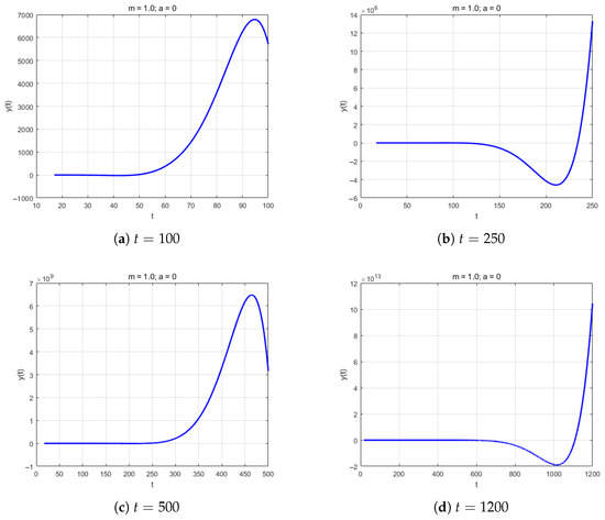
Figure 1. Numerical solutions demonstrating oscillatory behavior.

The numerical results clearly demonstrate that the solutions to the equation exhibit sustained oscillatory behavior when time t is sufficiently large, which aligns with the oscillation criteria established in this paper. It should be noted that the core focus of our theoretical work was to determine the oscillatory nature of the solutions, specifically whether the solutions possess arbitrarily large zeros. The boundedness of the solutions (i.e., whether the amplitude grows) is an independent mathematical issue. The amplitude growth observed in the numerical simulations precisely indicates the possibility of unbounded oscillatory solutions for the equation. This does not contradict the oscillatory conclusions of our study, but rather reveals the richer dynamical behaviors inherent in the system.

4. Results and Discussion Part

In this paper, we investigated the oscillations of a class of third-order neutral delay differential equations (Equation (5)). We extended the range of neutral coefficient $b\left(t\right)$ from $0\le b\left(t\right)\le 1$ to $b\left(t\right)\ge 1$, and also established the oscillation criteria for both the canonical and non-canonical cases. Not only do we provide examples to validate our criteria, but we also conducted numerical simulations that confirmed the sustained oscillatory behavior when t is sufficiently large. Therefore, our results extend and improve the oscillation theory for third-order neutral delay differential equations. This method can be used to study the oscillations of the following higher-order Emden–Fowler equation:

$${\left[a\left(t\right){\left({\chi }^{(n-1)}\left(t\right)\right)}^{\alpha }\right]}^{\prime }+c\left(t\right)y^{\beta }\left(h\left(t\right)\right)=0,$$

where n is odd and $\alpha \ne \beta$.

References

- Li, T.; Acosta-Soba, D.; Columbu, A.; Viglialoro, G. Dissipative gradient nonlinearities prevent δ-formations in local and nonlocal attraction-repulsion chemotaxis models. Stud. Appl. Math. 2025, 154, e70018. [Google Scholar] [CrossRef]
- Li, T.; Frassu, S.; Vigialoro, G. Combining effects ensuring boundedness in an attraction-repulsion chemotaxis model with production and consumption. Z. Angew. Math. Phys. 2023, 74, 109. [Google Scholar] [CrossRef]
- Kuramoto, Y.; Yamada, T. Trubulent state in chemical reaction. Prog. Theor. Phys. 1976, 56, 679–681. [Google Scholar] [CrossRef]
- Michelson, D. Steady solutions of the Kuramoto-Sivashinsky equation. Phys. D 1986, 19, 89–111. [Google Scholar] [CrossRef]
- Agarwal, R.; Bohner, M.; Li, T.; Zhang, C. Oscillation of third-order nonlinear delay differential equations. Taiwan J. Math. 2013, 17, 545–558. [Google Scholar] [CrossRef]
- Džurina, J.; Kotorová, R. Properties of the third order trinomial differential equations with delay argument. Nonlinear Anal. 2009, 71, 1995–2002. [Google Scholar] [CrossRef]
- Baculĺková, B. Properties of third-order nonlinear functional differential equations with mixed arguments. Abstr. Appl. Anal. 2011, 2011, 857860. [Google Scholar] [CrossRef]
- Baculĺková, B.; Džurina, J. On the asymptotic behavior of a class of third order nonlinear neutral differential equations. Cent. Eur. J. Math. 2010, 8, 1091–1103. [Google Scholar] [CrossRef]
- Baculĺková, B.; Džurina, J. Oscillation of third-order functional differential equations. Electron. J. Qual. Theory Differ. Equ. 2010, 43, 10–14232. [Google Scholar] [CrossRef]
- Baculĺková, B.; Džurina, J. Oscillation of third-order neutral differential equations. Math. Comput. Model. 2010, 52, 215–226. [Google Scholar] [CrossRef]
- Baculĺková, B.; Džurina, J. Oscillation of third-order nonlinear differential equations. Appl. Math. Lett. 2011, 24, 466–470. [Google Scholar] [CrossRef]
- Baculĺková, B.; Džurina, J.; Rogovchenko, Y. Oscillation of third order trinomial delay differential equations. Appl. Math. Comput. 2012, 218, 7023–7033. [Google Scholar] [CrossRef]
- Baculĺková, B.; Elabbasy, E.; Saker, S.; Džurina, J. Oscillation criteria for third-order nonlinear differential equations. Math. Slovaca 2008, 58, 201–220. [Google Scholar] [CrossRef]
- Candan, T.; Dahiya, R. Oscillation of third order functional differential equations with delay. Fifth Mississippi State Conference on Differential Equations and Computational Simulations. Electron. J. Differ. Equ. 2003, 10, 79–88. [Google Scholar]
- Candan, T.; Dahiya, R. Functional differential equations of third order. Electron. J. Differ. Equ. 2005, 12, 47–56. [Google Scholar]
- Džurina, J. Asymptotic properties of third order delay differential equations. Czechoslov. Math. J. 1995, 45, 443–448. [Google Scholar] [CrossRef]
- Džurina, J.; Grace, S.; Jadlovská, I. On nonexistence of Kneser solutions of third-order neutral delay differential equations. Appl. Math. Lett. 2019, 88, 193–200. [Google Scholar] [CrossRef]
- Došlá, Z.; Liška, P. Oscillation of third-order nonlinear neutral differential equations. Appl. Math. Lett. 2016, 56, 42–48. [Google Scholar] [CrossRef]
- Erbe, L. Existence of oscillatory solutions and asymptotic behavior for a class of third order linear differential equations. Pac. J. Math. 1976, 64, 369–385. [Google Scholar] [CrossRef]
- Elabbasy, E.; Hassan, T.; Elmatary, B. Oscillation criteria for third order delay nonlinear differential equations. Electron. J. Qual. Theory Differ. Equ. 2012, 5, 1–11. [Google Scholar] [CrossRef]
- Grace, S.; Agarwal, R.; Pavani, R.; Thandapani, E. On the oscillation of certain third order nonlinear functional differential equations. Appl. Math. Comput. 2008, 202, 102–112. [Google Scholar] [CrossRef]
- Grace, J.; Savithri, R.; Thandapani, E. Oscillatory properties of third order neutral delay differential equations. In Proceedings of the Fourth International Conference on Dynamical Systems and Differential Equations, Wilmington, NC, USA, 24–27 May 2002; pp. 342–350. [Google Scholar]
- Hanan, M. Oscillation criteria for third-order linear differential equations. Pac. J. Math. 1961, 11, 919–944. [Google Scholar] [CrossRef]
- Saker, S. Oscillation criteria of third-order nonlinear delay differential equations. Math. Slovaca 2006, 56, 433–450. [Google Scholar]
- Saker, S.; Džurina, J. On the oscillation of certain class of third-order nonlinear delay differential equations. Math. Bohem. 2010, 135, 225–237. [Google Scholar] [CrossRef]
- Tiryaki, A.; Aktaş, M. Oscillation criteria of a certain class of third order nonlinear delay differential equations with damping. J. Math. Anal. Appl. 2007, 325, 54–68. [Google Scholar] [CrossRef]
- Thandapani, E.; Li, T. On the oscillation of third-order quasi-linear neutral functional differential equations. Arch. Math. 2011, 47, 181–199. [Google Scholar]
- Jiang, Y.; Jiang, C.; Li, T. Oscillatory behavior of third-order nonlinear neutral delay differential equations. Adv. Differ. Equ. 2016, 2016, 171. [Google Scholar] [CrossRef]
- Li, T.; Rogovchenko, Y. On asymptotic behavior of solutions to higher-order sublinear Emden–Fowler delay differential equations. Appl. Math. Lett. 2017, 67, 53–59. [Google Scholar] [CrossRef]
- Li, T.; Zhang, C.; Baculícová, B.; Džurina, J. On the oscillation of third-order quasi-linear delay diffrential equations. Tatra Mt. Math. Publ. 2011, 48, 117–123. [Google Scholar]
- Li, T.; Rogovchenko, Y. On the asymptotic behavior of solutions to a class of third-order nonlinear neutral differential equations. Appl. Math. Lett. 2020, 105, 106293. [Google Scholar] [CrossRef]
- Jadlovská, I.; Li, T. A note on the oscillation of third-order delay differential equations. Appl. Math. Lett. 2025, 167, 109555. [Google Scholar] [CrossRef]
- Chatzarakis, G.; Grace, S.; Jadlovská, I.; Li, T.; Tunç, E. Oscillation criteria for third-order Emden–Fowler differential equations with unbounded neutral coefficients. Complexity 2019, 2019, 5691758. [Google Scholar] [CrossRef]
- Kiguradze, I.; Chanturia, T. Asymptotic properties of solutions of nonautonomous ordinary differential equations. In Mathematics and Its Applications; Kluwer Academic Publishers Group: Dordrecht, The Netherlands, 1993. [Google Scholar]
- Philos, C. On the existence of nonoscillatory solutions tending to zero at ∞ for differential equations with positive delays. Arch. Math. 1981, 36, 168–178. [Google Scholar] [CrossRef]
- Koplatadze, R.; Chanturiya, T. Oscillating and monotone solutions of first-order differential equations with deviating argument. Differ. Uravn. 1982, 18, 1463–1465. [Google Scholar]
- Kitamura, Y.; Kusano, T. Oscillation of first-order nonlinear differential equations with deviating arguments. Proc. Am. Math. Soc. 1980, 78, 64–68. [Google Scholar] [CrossRef]
- Zhang, S.-Y.; Wang, Q.-R. Oscillation of second-order nonlinear neutral dynamic equations on time scales. Appl. Math. Comput. 2010, 216, 2837–2848. [Google Scholar] [CrossRef]
Disclaimer/Publisher’s Note: The statements, opinions and data contained in all publications are solely those of the individual author(s) and contributor(s) and not of MDPI and/or the editor(s). MDPI and/or the editor(s) disclaim responsibility for any injury to people or property resulting from any ideas, methods, instructions or products referred to in the content. |
© 2025 by the authors. Licensee MDPI, Basel, Switzerland. This article is an open access article distributed under the terms and conditions of the Creative Commons Attribution (CC BY) license (https://creativecommons.org/licenses/by/4.0/).