Exact Solutions for Strong Nonlinear Oscillators with Linear Damping

Abstract

This paper presents the derivation of an exact solution for a damped nonlinear oscillator of arbitrary order (both integer and non-integer). A coefficient relationship was defined under which such a solution exists. The analytical procedure was developed based on the application of the Ateb (inverse beta) function. It has been shown that an exact solution exists for a specific relationship between the damping coefficient and the coefficient of the linear elastic term, and that this relationship depends on the order of nonlinearity. The exact amplitude of vibration was found to be a time-decreasing function, depending on the initial amplitude, damping coefficient, and the order of nonlinearity. The period of vibration was also shown to depend not only on the amplitude but also on both the nonlinearity coefficient and its order. For cases where the damping coefficient of the exact oscillator is slightly perturbed, an approximate solution based on the exact one was proposed. Three illustrative examples of oscillators with different orders of nonlinearity were considered: a nearly linear oscillator, a Duffing oscillator, and one with strong nonlinearity. For all cases, the high accuracy of the asymptotic solution was confirmed. Since no exact analytic solution exists for a purely nonlinear damped oscillator, an approximate solution was constructed using the solution of the corresponding undamped oscillator with a time-varying amplitude and phase. In the case of a purely cubic damped oscillator, the approximate solution was compared with numerical results, and good agreement was demonstrated.

1. Introduction

It is well known that a physically realistic description of an oscillator’s dynamics is impossible without including system nonlinearity and damping. To accurately capture these effects, oscillators must be modeled using differential equations with nonlinearity of integer or non-integer order and a linear damping term [1]. The introduction of damping makes the system non-conservative, and in most cases, the equation of motion becomes non-integrable and lacks an exact analytical solution [2]. As a result, numerous approximate methods have been developed for solving nonlinear differential equations with damping.

A significant body of research has been dedicated to the Duffing equation with linear damping, which serves as a model for the dynamic behavior of oscillators in mechanical systems and structures [3,4], as well as in discharge lamps [5], plasma physics [6], rigid rotators [7], and centrifugal governors [8]. Most solution techniques are semi-analytic [9,10], relying on perturbative approaches such as the method of multiple scales, renormalization, and parameter variation. However, these techniques are generally applicable only to limited cases. For instance, the Differential Transformation Method (DTM) [11] provides solutions over a short time span, while the Modified DTM (MDTM) [12,13] extends applicability to longer intervals, albeit for specific parameter values and initial conditions, thus limiting generalization. An improved semi-analytic technique combining harmonic balance, parameter bookkeeping, and Newton’s method has been proposed in [14], allowing for oscillators with both even and odd nonlinearities, including systems without a linear restoring force. This method has also been successfully applied to the non-integrable cubic–quintic Duffing equation with linear damping [15]. Mandal [16] introduced a more accurate, though complex, perturbation technique based on unknown parameters determined through coefficient comparison. To address these complexities, He’s frequency–amplitude formulation and energy balance method were proposed, although they deviate from numerical results. A more suitable analytical framework is based on the Fourier series [17] and higher-order homotopy techniques [18]. In [19], the application of the proposed methods to a pure nonlinear oscillator with linear damping yielded qualitatively correct results. To improve quantitative agreement, the solution was expressed via Jacobi elliptic functions. However, their applicability is confined to oscillators with quadratic and cubic nonlinearities [20,21,22,23,24]. Panayotounakos et al. [25] introduced a methodology for the damped pure cubic oscillator based on iterative solutions of nonlinear transcendental equations. Although implicit, this approach suggests a promising direction in the quest for exact solutions. Exact analytical solutions for damped nonlinear oscillators remain rare and are typically constrained to specific orders of nonlinearity and parameter values. For example, exact solutions are available for the damped Duffing oscillator when $c_1=\sqrt{2}b/3$ [26] and for the damped quantic oscillator when $b=4c_1/\sqrt{3}$ [27], where $c_1$ denotes the linear elastic coefficient and b denotes the damping coefficient. These solutions show that the amplitude depends solely on damping and is independent of elastic coefficients. Using Lie symmetry theory, Almendral and Sanjuán [28] proved the integrability of the damped quadratic Helmholtz oscillator under specific parameter choices, yielding solutions in hyperbolic and Jacobian elliptic forms [29]. Similarly, Sales et al. [30] derived an exact solution in the Weierstrass elliptic form for the damped quadratic oscillator under restricted initial conditions. An exact solution for the Duffing–Helmholtz oscillator is found under the relation $c_1^2={\displaystyle \frac{3c_2^4+2b^2{c}_3^2}{9c_3^2}}$, involving coefficients of linear, quadratic, and cubic terms. Nonetheless, exact analytic solutions for oscillators with other nonlinearities are yet to be established.

The main objective of this paper is to generalize the derivation of exact solutions for damped nonlinear oscillators of arbitrary order—integer or non-integer—and to define coefficient relations for which such equations are integrable. The paper is structured as follows: After the Introduction and Preliminary sections, Section 3 presents the exact solution in terms of the Ateb function for a system with a specific damping coefficient, including amplitude decay and period variation analysis. Section 4 analyzes systems with damping coefficients near the exact value and applies the method of time-dependent amplitude and phase. Section 5 considers a purely nonlinear oscillator with linear damping and uses an energy-based approach to obtain an approximate solution. After the Discussion in Section 6, the paper ends with Conclusions, with a summary of findings and implications.

2. Preliminary

This study investigates a class of damped nonlinear oscillators of arbitrary order, encompassing both integer and non-integer powers in the restoring force. The model of the strong nonlinear oscillator with linear damping considered in the paper is

$$\ddot{x}+c_{\alpha }^{2}x{\left|x\right|}^{\alpha -1}+c_1^{2}x+b\dot{x}=0,$$

(1)

where $x=x(t)$ denotes the displacement of the system, which is a function of time t, $c_1^2$ and $c_{\alpha }^2$ are the linear and nonlinear system parameters, respectively, α $\ge$ 1, α $\in \mathbb{R}$ is the order of nonlinearity, and b is the coefficient of the linear damping. For α $=$ 1, Equation (1) simplifies into a linear one. Equation (1) is assumed to be dimensionless.

The analytical solving method is based on the application of the Ateb function (inverse beta function), which generalizes trigonometric functions and is particularly suitable for modeling nonlinear oscillatory behavior with amplitude and period variations. (More about the Ateb function is presented in Appendix A) The solution of (1) is thought to be in the form of

$$x=A\exp (-\delta t) ca(\alpha ,1,\omega \exp (-\beta \delta t)+{\psi }_0),$$

(2)

where ca is the cosine Ateb function [30], ω, δ, and β are unknown parameters that satisfy Equation (1), and A and ${\psi }_0$ are arbitrary constants that have to satisfy the initial conditions:

$$x(0)=x_0, \dot{x}(0)={\dot{x}}_0.$$

(3)

Remark 1.

The background of Ateb functions is given in Appendix A.

Using relations (2) and (A4), the first and second time derivatives are obtained:

$$\dot{x}=-\delta A\exp (-\delta t)ca+\mathit{\omega }\mathit{\delta }\mathit{\beta }\exp (-(1+\beta )\delta t){\displaystyle \frac{2}{\alpha +1}}Asa,$$

(4)

$$\ddot{x}={\delta }^{2}A\exp (-\delta t)ca-\omega \beta (2+\beta ){\delta }^2\exp (-(1+\beta )\delta t){\displaystyle \frac{2}{\alpha +1}}sa-{\omega }^2{\delta }^2{\beta }^2\exp (-(1+2\beta )\delta t){\displaystyle \frac{2}{\alpha +1}}c{a}^{\alpha },$$

(5)

where $ca=ca(\alpha ,1,\omega \exp (-\beta \delta t)+{\psi }_0)$ and $sa=sa(1,\alpha ,\omega \exp (-\beta \delta t)+{\psi }_0)$. After substituting (2), (4), and (5) into (1) and separating the terms with the same functions, the following relations are obtained:

$$c{a}^{\alpha }:-{\displaystyle \frac{2}{\alpha +1}}{\omega }^2{\delta }^2{\beta }^2\exp (-(1+2\beta )\delta t)+c_{\alpha }^2{A}^{\alpha -1}\exp (-\alpha \delta t)=0,$$

(6)

$$sa:\hspace{1em}-\delta (2+\beta )+b=0,$$

(7)

$$ca:\hspace{1em}{\delta }^2+c_1^2-b\delta =0,$$

(8)

After solving Equations (6) and (7), parameters ω, δ, and β are as follows:

$$\beta ={\displaystyle \frac{\alpha -1}{2}},\hspace{1em}\hspace{1em}\delta ={\displaystyle \frac{b}{2+\beta }}={\displaystyle \frac{2b}{\alpha +3}},\hspace{1em}\hspace{1em}\omega \delta \beta =c_{\alpha }\sqrt{{\displaystyle \frac{\alpha +1}{2}}}{A}^{(\alpha -1)/2}.$$

(9)

By solving (8), the restrictive relation between a certain damping coefficient $b_e$ and the coefficient of the linear elastic term c₁ is obtained as

$$b_e=c_1{\displaystyle \frac{\alpha +3}{\sqrt{2(\alpha +1)}}} .$$

(10)

For condition (10), Equation (1) has an exact analytic solution. Relation (10) depends on the order of nonlinearity.

Table 1. $b_e/c_1$ for various values of $\alpha$.

$\mathit{\alpha }$	1.1	2	3	5	7
$b_e/c_1$	${\displaystyle \frac{4.1}{\sqrt{4.2}}}=2.0006$	${\displaystyle \frac{5}{\sqrt{6}}}=2.0412$	${\displaystyle \frac{3}{\sqrt{2}}}=2.1213$	${\displaystyle \frac{4}{\sqrt{3}}}=2.3094$	${\displaystyle \frac{5}{2}}=2.5000$

presents the computed values of $b_e/c_1$ for various values of $\alpha$.

Data in Table 1 for quadratic, cubic, and quantic oscillators agree with those already published [26,29]. The $b_e/c_1$ ratio increases with $\alpha$.

In this paper, an exact analytical solution for (1) is derived for a specific relationship between the damping coefficient and the linear stiffness coefficient (10), which is a relationship that explicitly depends on the order of nonlinearity. It is demonstrated that the exact amplitude of vibration is a time-decreasing function influenced by the initial amplitude, the damping coefficient, and the order of nonlinearity, while being independent of the linear stiffness coefficient. The decay in amplitude is more rapid in systems with lower-order nonlinearity and becomes slower as the order increases.

Furthermore, the period of oscillation is shown to be time-dependent and to increase as a function of both the amplitude and the order of nonlinearity. In contrast to the linear case, where the period remains constant, nonlinear systems exhibit a growing period over time, with the growth rate increasing with higher orders of nonlinearity.

For cases in which the damping coefficient slightly deviates from the exact value, an approximate solution is constructed by perturbing the exact one. This approximation remains valid and accurate for moderate variations in the damping parameter. Three representative examples are examined to validate the method: a nearly linear oscillator, a Duffing-type oscillator, and a strongly nonlinear oscillator. In each case, the proposed analytical or asymptotic solution shows excellent agreement with numerical results.

Since an exact solution is not available for a purely nonlinear damped oscillator (i.e., one without a linear elastic term), an approximate solution is constructed using the known solution of the corresponding undamped system. This solution incorporates time-dependent amplitude and phase and successfully captures the qualitative behavior of the system. For the specific case of a damped cubic oscillator, the approximate solution shows good agreement with numerical simulations.

This preliminary analysis lays the groundwork for the detailed derivation and validation of exact and approximate solutions presented in the following sections.

3. Exact Analytic Solution of a Linearly Damped Nonlinear Oscillator

3.1. Exact Solution

For the parameter relation (10) and $\beta ={\displaystyle \frac{\alpha -1}{2}},$ the expressions for $\delta$ and $\omega$ in (9) are transformed into

$$\delta =c_1\sqrt{{\displaystyle \frac{2}{\alpha +1}}},\hspace{1em}\hspace{1em}\hspace{1em}\hspace{1em}\hspace{1em}\omega ={\displaystyle \frac{c_{\alpha }}{c_1}}{\displaystyle \frac{\alpha +1}{\alpha -1}}{A}^{(\alpha -1)/2}.$$

(11)

Using (9)–(11), it follows that Equation (1)

$$\ddot{x}+c_{\alpha }^{2}x{\left|x\right|}^{\alpha -1}+c_1^{2}x+(c_1{\displaystyle \frac{\alpha +3}{\sqrt{2(\alpha +1)}}})\dot{x}=0,$$

(12)

has the exact solution of

$$x=A\exp \left(-c_{1}t\sqrt{{\displaystyle \frac{2}{\alpha +1}}}\right)ca\left( \alpha ,1, {\displaystyle \frac{c_{\alpha }}{c_1}}{\displaystyle \frac{\alpha +1}{\alpha -1}}(A \mathrm{e}\mathrm{x}\mathrm{p}(-c_{1}t\sqrt{{\displaystyle \frac{2}{\alpha +1}})}{)}^{{\displaystyle \frac{\alpha -1}{2}}}+{\psi }_0\right).$$

(13)

For initial conditions $x(0)=A_0$ and $\dot{x}(0)=-A_0\delta ,$ when the initial amplitude is $A(0)=A_0$ ($A_0>0$) and the phase shift is ${\psi }_0={\displaystyle \frac{c_{\alpha }}{c_1}}{\displaystyle \frac{\alpha +1}{\alpha -1}}{A}_0^{{\displaystyle \frac{\alpha -1}{2}}}$, the x-t expression (13) is

$$x=A_0\exp \left(-c_{1}t\sqrt{{\displaystyle \frac{2}{\alpha +1}}}\right)ca\left( \alpha ,1, {\displaystyle \frac{c_{\alpha }}{c_1}}{\displaystyle \frac{\alpha +1}{\alpha -1}}{A}_0^{{\displaystyle \frac{\alpha -1}{2}}}(1-\exp \left(-c_1{\displaystyle \frac{\alpha -1}{2}}t\sqrt{{\displaystyle \frac{2}{\alpha +1}}}\right))\right),$$

(14)

In other words, according to (10), then

$$x=A_0 \exp \left(-{\displaystyle \frac{2b_{e}t}{\alpha +3}}\right) ca(\alpha ,1, {\displaystyle \frac{c_1}{b_e^2}}{\displaystyle \frac{\alpha +3}{(\alpha -1)\sqrt{2(\alpha +1)}}}\sqrt{c_{\alpha }^2{\displaystyle \frac{\alpha +1}{2}}}{A}_0^{{\displaystyle \frac{\alpha -1}{2}}}(1-\exp \left(-{\displaystyle \frac{b_e(\alpha -1)t}{\alpha +3}}\right)).$$

(15)

3.2. Amplitude of Vibration Under Damping

After analyzing relations (14) and (15), it is evident that the amplitude of oscillation is

$${A_a(t)=A}_0 \mathrm{e}\mathrm{x}\mathrm{p}(-c_{1}t\sqrt{{\displaystyle \frac{2}{\alpha +1}}}),\hspace{1em}\hspace{1em}\mathrm{i}.\mathrm{e}.,\hspace{1em}\hspace{1em}{A}_a(t)=A_0 \exp \left(-{\displaystyle \frac{2b_{e}t}{\alpha +3}}\right).$$

(16)

The amplitude of vibration is the product of the initial amplitude $A_0$ and the damping function $\exp \left(-{\displaystyle \frac{2b_{e}t}{\alpha +3}}\right)$, i.e., $(-c_{1}t\sqrt{{\displaystyle \frac{2}{\alpha +1}}})$. The damping function depends on the coefficient $b_e$, but also on the order of nonlinearity $\alpha$. In

Table 2. The A/A₀ ratio for various values of α.

$\mathit{\alpha }$	1.1	2	3	5	7
$A_a/A_0$	$\exp \left(-{\displaystyle \frac{20b_{e}t}{41}}\right)$	$\exp \left(-{\displaystyle \frac{2b_{e}t}{5}}\right)$	$\exp \left(-{\displaystyle \frac{b_{e}t}{3}}\right)$	$\exp \left(-{\displaystyle \frac{b_{e}t}{4}}\right)$	$\exp \left(-{\displaystyle \frac{b_{e}t}{5}}\right)$

, the amplitude ratio $A_a/A_0$ for various values of $\alpha$ is shown.

The amplitude–time functions for the damped linear, quadratic, and cubic nonlinear oscillators, presented in Table 2, agree with those already published [25,28]. Based on the results shown in (16) and in Table 2, it is concluded that the amplitude decrease is the fastest for the linear oscillator when α = 1. The higher the order of nonlinearity $\alpha$ is, the slower the amplitude decrease is. If the order of nonlinearity tends to infinity (α $\to \infty$), the amplitude tends to the constant value of the initial amplitude $A_0$. In addition, it is worth mentioning that the amplitude–time function (16) is independent of the coefficient of the nonlinearity $c_{\alpha }$.

3.3. Exact Period of Vibration

In (13), it is seen that the argument of the ca function depends on ${\displaystyle \frac{c_{\alpha }}{c_1}}{\displaystyle \frac{\alpha +1}{\alpha -1}}{A}_a^{{\displaystyle \frac{\alpha -1}{2}}}$, where $A_a$ is the amplitude function (16), $\alpha$ is the order of nonlinearity, and $c_1^2$ and $c_{\alpha }^2$ are coefficients of the linear and nonlinear deflection terms, i.e., the argument varies in time according to an exponential function. Due to this fact, it is obvious that the ca Ateb function with this argument has period intervals that vary in time. For their derivations, the periodic property of the ca function is applied. Namely, after rewriting the ca function in (16) into $ca(\alpha ,1,\omega (1-\exp (-\beta \delta t))$ with $\beta \delta =c_1{\displaystyle \frac{\alpha -1}{\sqrt{2(\alpha +1)}}}$ and $\omega ={\displaystyle \frac{c_{\alpha }}{c_1}}{\displaystyle \frac{\alpha +1}{\alpha -1}}{A}_0^{{\displaystyle \frac{\alpha -1}{2}}}$, and utilizing the period of the ca function [31], the following is obtained:

$$2\mathsf{\Pi }=2B\left({\displaystyle \frac{1}{\alpha +1}},{\displaystyle \frac{1}{2}}\right)=2{\displaystyle \frac{\mathsf{\Gamma }(\frac{1}{\alpha +1})\mathsf{\Gamma }(\frac{1}{2})}{\mathsf{\Gamma }(\frac{\alpha +3}{2(\alpha +1)})}},$$

(17)

where B is the complete beta function and $\mathsf{\Gamma }$ is the gamma function [32]; the characteristic time intervals T_i are computed according to

$$\omega (1-\exp (-\beta \delta T_i))={\displaystyle \frac{\mathsf{\Pi }}{2}}i,$$

(18)

where i = 1, 2, 3, …. After some modification, the following is obtained:

$${\mathit{T}}_i={\displaystyle \frac{1}{\beta \delta }}ln\left|{\displaystyle \frac{2\omega }{2\omega -i\mathsf{\Pi }}}\right|.$$

(19)

Expression (19) gives the exact values of the periods and their variations. Thus, the periods of vibration are

$$T_I=T_4-T_0,\hspace{1em}\hspace{1em}{T}_{II}=T_8-T_4,\hspace{1em}\hspace{1em}{T}_{III}=T_{12}-T_8 \dots .T_J=T_{4J}-T_{4(J-1)},$$

(20)

where $T_0=0$, J = 1, 2, 3, …. The period variation is calculated using the relation

$$T_{J+1,J}\%={\displaystyle \frac{T_{J+1}-T_J}{T_J}}100\%.$$

(21)

The calculated periods of the ca function correspond to periods of vibration of the damped oscillator.

Remark 2.

If damping is omitted, the argument ca function is the linear time function, and the period is constant [30].

3.4. First Integral for the Integrable Equation

For the condition (12) equation,

$$\ddot{x}+b_e\dot{x}+c_{\alpha }^{2}x{\left|x\right|}^{\alpha -1}+{\displaystyle \frac{2b_e^2(\alpha +1)}{(\alpha +3{)}^2}}x=0,$$

(22)

has the first integral, which is derived as

$$\exp \left({\displaystyle \frac{2b_{e}t(\alpha +1)}{\alpha +3}}\right)[{\displaystyle \frac{1}{2}}(\dot{x}+{\displaystyle \frac{2b_e}{\alpha +3}}x{)}^2+c_{\alpha }^2{\displaystyle \frac{x^{\alpha +1}}{\alpha +1}}]=I_0=const.,$$

(23)

In other words,

$$\exp (c_{1}t\sqrt{2(\alpha +1)})\left({\displaystyle \frac{1}{2}}(\dot{x}+{\displaystyle \frac{{2c}_1}{\sqrt{2(\alpha +1)}}}x{)}^2+c_{\alpha }^2{\displaystyle \frac{x^{\alpha +1}}{\alpha +1}}\right)=I_0=const.,$$

(24)

where $I_0$ is a constant value dependent on the initial conditions.

Remark 3.

For the special case, when the nonlinearity is cubic ($\alpha =3$ ) and $b_e={\displaystyle \frac{3c_1}{\sqrt{2}}}$, the first integral (23) is

$$\exp \left({\displaystyle \frac{4b_{e}t}{3}}\right)[{\displaystyle \frac{1}{2}}(\dot{x}+{\displaystyle \frac{b_e}{3}}x{)}^2+c_{\alpha }^2{\displaystyle \frac{x^4}{4}}]=I_0=const.,$$

(25)

while for the quadratic nonlinearity ($\alpha =2$) and $b_e={\displaystyle \frac{5c_1}{\sqrt{6}}}$, it is

$$\exp \left({\displaystyle \frac{6b_{e}t}{5}}\right)[{\displaystyle \frac{1}{2}}(\dot{x}+{\displaystyle \frac{2b_e}{5}}x{)}^2+c_{\alpha }^2{\displaystyle \frac{x^3}{3}}]=I_0=const.$$

(26)

The main relevance of the first integral is its easier solving of the damped nonlinear oscillators. For computational reasons, it is suitable to rewrite (23) into

$${\displaystyle \frac{1}{2}}(\dot{x}+{\displaystyle \frac{2b_e}{\alpha +3}}x{)}^2+c_{\alpha }^2{\displaystyle \frac{x^{\alpha +1}}{\alpha +1}}-I_0\exp \left(-{\displaystyle \frac{2b_{e}t(\alpha +1)}{\alpha +3}}\right)=0.$$

(27)

Thus, one of the non-oscillatory particular solutions for (27) is as follows:

$$x=({\displaystyle \frac{I_0(\alpha +1)}{c_{\alpha }^2}}{)}^{{\displaystyle \frac{1}{\alpha +1}}}\exp \left(-{\displaystyle \frac{2b_{e}t}{\alpha +3}}\right).$$

(28)

The decrease in x in time corresponds to amplitude decreases in $A_a(t)$ (16).

The first integral is complex but suitable for deriving the initial amplitude $A_0$ related to initial deflection $x_0$ and initial velocity ${\dot{x}}_0$. When substituting solution (13) into (24), the initial amplitude is

$$A_0=({\displaystyle \frac{I_0}{c_{\alpha }^2}}{\displaystyle \frac{\alpha +1}{2}}{)}^{{\displaystyle \frac{1}{\alpha +1}}},$$

(29)

where for $x(0)=0,{\dot{x}(0)=\dot{x}}_0$, the constant is $I_0={\displaystyle \frac{1}{2}}{\dot{x}}_0^2$, and for $x(0)=x_0,\dot{x}(0)=0$, the first integral is $I_0={\displaystyle \frac{1}{\alpha +1}}(c_1^2{x}_0^2+c_{\alpha }^2{x}_0^{\alpha +1})$.

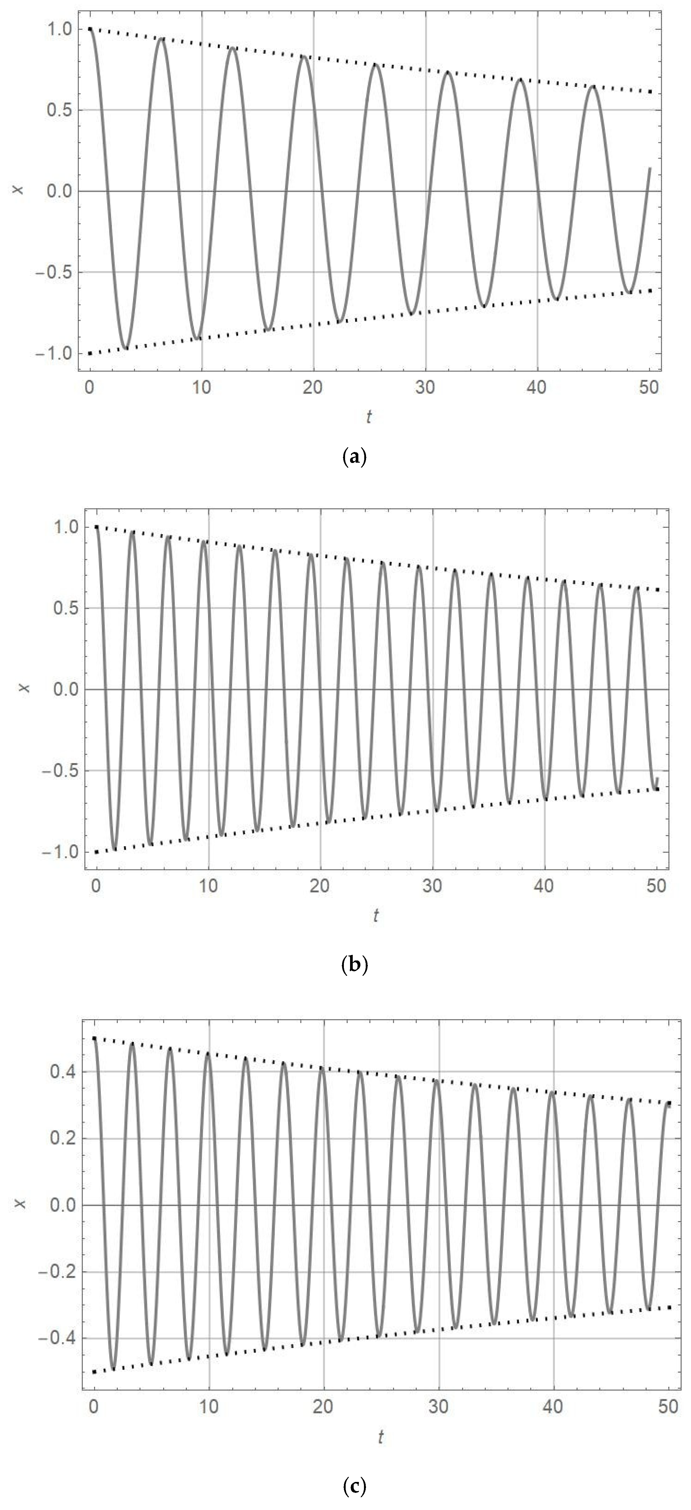
3.5. Example 1: Oscillators of Order of Nonlinearity α = 1.1; 3; 7

As an example, three differential equations with various orders of nonlinearity are considered: an almost linear one ($\alpha =1.1)$, the Duffing one $(\alpha =3)$, and one of the seventh order $(\alpha =7)$. For these values, Equation (14) yields

$$\mathrm{for} \alpha =1.1:\hspace{1em}\hspace{1em}\ddot{x}+c_{\alpha }^{2}x{\left|x\right|}^{0.1}+c_1^{2}x+2c_1\dot{x}=0,$$

$$\mathrm{for} \alpha =3:\hspace{1em}\hspace{1em}\ddot{x}+c_{\alpha }^{2}x{\left|x\right|}^2+c_1^{2}x+2.1\dot{x}=0,$$

$$\mathrm{for} \alpha =7:\hspace{1em}\hspace{1em}\ddot{x}+c_{\alpha }^{2}x{\left|x\right|}^6+c_1^{2}x+2.5c_1\dot{x}=0$$

with initial conditions of $x(0)=A_0,\dot{x}(0)=-\delta A_0$.

The exact analytic solution of the aforementioned equations is in accordance with (15):

$$\mathrm{for} \alpha =1.1:\hspace{1em}\hspace{1em}x=A_{a}ca(1.1,1,21{\displaystyle \frac{c_{\alpha }}{c_1}}{(A_0\exp (-0.9759c_{1}t))}^{0.05}+{\psi }_0)$$

where $A_a=A_0\exp (-0.9759c_{1}t)$, $\delta =0.9759c_1$.

$$\mathrm{for} \alpha =3:\hspace{1em}\hspace{1em}x=A_{a}ca(3,1,2{\displaystyle \frac{c_{\alpha }}{c_1}}(A_0\exp (-0.7071c_{1}t))+{\psi }_0)$$

where $A_a=A_0\exp (-0.7071c_{1}t)$, $\delta =0.7071c_1$.

$$\mathrm{for} \alpha =7:\hspace{1em}\hspace{1em}x=A_{a}ca(7,1,1.33{\displaystyle \frac{c_{\alpha }}{c_1}}{(A_0\exp (-0.5c_{1}t))}^3+{\psi }_0)$$

where $A_a=A_0\exp (-0.5c_{1}t)$, $\delta =0.5c_1$.

In Figure 1, Figure 2 and Figure 3, the obtained x-t response is plotted. The coefficients are $c_1=0.01$ and (a) $c_{\alpha }=1$, $A_0=1$; (b) $c_{\alpha }=2$, $A_0=1$; (c) $c_{\alpha }=2$, $A_0=0.5$; and (d) $c_{\alpha }=2$, $A_0=2$. In Figure 1, Figure 2 and Figure 3, the analytically obtained $A_a-t$ diagrams are plotted.

Analyzing Figure 1, Figure 2 and Figure 3 and Equation (16), the conclusion about amplitude decay rates for various values of α is obtained: the higher the order of nonlinearity, the slower the amplitude decay. For extremely high orders of nonlinearity ($\alpha \to \infty$), the amplitude decay may be omitted, and the amplitude of vibration is almost constant and tends to the initial amplitude ($A\to A_0$).

According to (21)–(23), in

Table 3. Periods of vibration for the oscillators of the orders of α =1.1, 3, and 7.

	$\mathit{\alpha }=1.1$	$\mathit{\alpha }=3$	$\mathit{\alpha }=7$
$\mathsf{\Pi }$	$3.2502$	$5.2441$	$9.3087$
$T_i$	$2049.4ln\left|{\displaystyle \frac{4400}{4400-3.2502i}}\right|$	$141ln\left|{\displaystyle \frac{400}{400-5.2441i}}\right|$	${\displaystyle \frac{200}{3}}ln\left|{\displaystyle \frac{800/3}{\frac{800}{3}-9.3087i}}\right|$
$T_1$	1.5144	1.8606	2.3688
$T_2$	3.0299	3.7464	4.8248
$T_3$	4.5466	5.6576	7.3748
$T_4$	6.0644	7.5951	10.026
$T_5$	7.5833	9.5596	12.787
$T_6$	9.1033	11.552	15.668
$T_7$	9.6240	13.573	18.679
$T_8$	12.147	15.623	21.832
$T_9$	13.670	17.703	25.142
$T_{10}$	15.195	19.815	28.624
$T_{11}$	16.720	21.958	32.299
$T_{12}$	18.247	24.135	38.188
$T_{13}$	19.775	26.346	40.318
$T_{14}$	21.304	28.592	44.721
$T_{15}$	22.835	30.875	49.435
$T_{16}$	24.366	33.195	54.508
$T_I$	6.0644	7.5951	10.026
$T_{II}$	6.0826	8.143	12.355
$T_{III}$	6.1000	8.643	15.176
$T_{IV}$	6.1190	9.060	16.320
$T_{II,I}\%$	0.300%	5.772%	18.59%
$T_{III,II}\%$	0.306%	6.135%	22.83%
$T_{IV,III}\%$	0.311%	6.825%	27.54%

, the time intervals, periods, and period variations for oscillators of the orders of $\alpha =1.1$, $\alpha =3$, and $\alpha =7$ are presented. The parameters of the oscillator are $c_1=0.01$, $c_{\alpha }=1$, and the initial amplitude is $A_0=1$. The first four ‘periods’ of vibration and their variation in time are calculated.

Comparing the diagrams in Figure 1, Figure 2 and Figure 3 and analyzing the data in Table 3 given for various orders of nonlinearity α and certain values of $c_1$, $c_{\alpha }$ and initial amplitude $A_0$, it is obtained that the amplitude decrease is slower for α = 7 than for α = 3 and α = 1.1. For initial amplitude $A_0\le 1$, the period of vibration is the longest for α = 7, shorter for α = 3, and the shortest for α = 1.1. On the other hand, if the initial amplitude is $A>1$, the frequency of vibration is the highest for α = 7, lower for α = 3, and the lowest for α = 1.1. Analyzing the data in Table 3, it is obvious that the period of vibration for the oscillator, which is close to a linear one ($\alpha =1.1$), is almost constant and its variation in time is smaller than 1%. When increasing the order of nonlinearity ($\alpha =3)$, the period of vibrations is longer and its change in time is faster. For the oscillator with a high order of nonlinearity ($\alpha =7)$, the periods of vibration are more than two times longer than those of linear ones and their increase is extremely high.

4. Approximate Solution for Almost-Exact Strong Nonlinear Oscillator with Linear Damping

Unfortunately, there is no exact analytical solution for the oscillator with any order of nonlinearity and linear damping. If the damping coefficient differs from the value $b_e$ (10) for $\epsilon \ll 1$, it is assumed that the approximate solution for the differential equation of motion, as follows,

$$\ddot{x}+c_{\alpha }^{2}x{\left|x\right|}^{\alpha -1}+c_1^{2}x+{(b}_e\pm \epsilon )\dot{x}=0,$$

(30)

has to be close to solution (13) of Equation (12).

Remark 4.

The parameter $\epsilon$ may be positive or negative. For simplification, the solving procedure is carried out only for the negative value of $\epsilon$, when the total damping coefficient b is ${(b}_e-\epsilon )$ Then, the corresponding Equation (30) is

$$\ddot{x}+c_{\alpha }^{2}x{\left|x\right|}^{\alpha -1}+c_1^{2}x+b_e\dot{x}=\epsilon \dot{x}.$$

(31)

Equation (31) differs from (14) for the small damping term $\epsilon \dot{x}$. It suggests that the solution of (31) is the perturbed version of the exact solution (13), i.e., that the solution and the first derivative of (31) have the form of (2) and (4) but with time-variable amplitudes A(t) and phase modulations $\psi (t)$ of the ca Ateb function:

$$x=A(t)\exp (-\delta t)ca(\alpha ,1,\omega (t)\exp (-\beta \delta t)+\psi (t)),$$

(32)

$$\dot{x}=-\delta A(t)\exp (-\delta t)ca+\omega (t)\mathit{\delta }\mathit{\beta }\exp (-(1+\beta )\delta t){\displaystyle \frac{2}{\alpha +1}}A(t)sa$$

(33)

Here,

$$\omega (t)={\displaystyle \frac{c_{\alpha }}{c_1}}{\displaystyle \frac{\alpha +1}{\alpha -1}}{(A(t))}^{{\displaystyle \frac{\alpha -1}{2}}}.$$

(34)

Comparing the time derivative of (32) with the assumed expression (33), the constraint is as follows:

$$\dot{A}ca-{\displaystyle \frac{2}{\alpha +1}}A\dot{\psi } sa=0.$$

(35)

After substituting (32), (33), and the time derivative of (33) into (31), and after some modifications, the following is obtained:

$$\begin{gathered} -\dot{A}ca+{\displaystyle \frac{2}{\alpha +1}}A\dot{\psi }sa+(\dot{A}\omega +A\dot{\omega })\beta \exp (-\beta \delta t){\displaystyle \frac{2}{\alpha +1}}sa \\ +A\dot{\psi }\mathit{\omega }\mathit{\beta }\exp (-\beta \delta t){\displaystyle \frac{2}{\alpha +1}}{ca}^{\alpha } \\ =\epsilon (-Aca+\mathit{\omega }\mathit{\beta }\exp (-\beta \delta t){\displaystyle \frac{2}{\alpha +1}}Asa), \end{gathered}$$

(36)

Here,

$$\dot{A}\omega +A\dot{\omega }=\dot{A}\omega {\displaystyle \frac{\alpha +1}{2}}.$$

(37)

Substituting Equation (36) into (37), we obtain

$$\begin{gathered} -\dot{A(}ca-\mathit{\omega }\mathit{\beta }\exp (-\beta \delta t)sa)+{\displaystyle \frac{2}{\alpha +1}}A\dot{\psi }(sa+\mathit{\omega }\mathit{\beta }\exp (-\beta \delta t){ca}^{\alpha }) \\ =\epsilon (-Aca+\mathit{\omega }\mathit{\beta }\exp (-\beta \delta t){\displaystyle \frac{2}{\alpha +1}}Asa). \end{gathered}$$

(38)

After some transformations, Equations (35) and (38) become

$$\dot{A} \mathit{\omega }\mathit{\beta }\exp (-\beta \delta t)=\epsilon \left(-Acasa+A\mathit{\omega }\mathit{\beta }\exp (-\beta \delta t){\displaystyle \frac{2}{\alpha +1}}{sa}^2\right),$$

(39)

$$\dot{\psi }\omega ={\displaystyle \frac{\alpha +1}{\alpha -1}}\epsilon \left(-c{a}^2\mathrm{e}\mathrm{x}\mathrm{p}(\beta \delta t)+\mathit{\omega }\mathit{\beta }{\displaystyle \frac{2}{\alpha +1}}sa ca\right).$$

(40)

Equations (39) and (40) represent the two first-order coupled ones, which correspond to (33). Unfortunately, there is no closed-form analytic solution for the system of Equations (39) and (40). At this point, the procedure of averaging [30] the periodic Ateb functions over their period of vibration is introduced. The averaged Equations (39) and (40) become

$$\dot{A} \mathit{\omega }\mathit{\beta }\exp (-\beta \delta t)=\epsilon \left(-A〈casa〉+A\mathit{\omega }\mathit{\beta }\exp (-\beta \delta t){\displaystyle \frac{2}{\alpha +1}}\langle {sa}^2\rangle \right),$$

(41)

$$\dot{\psi }\omega ={\displaystyle \frac{\alpha +1}{\alpha -1}}\epsilon \left(-\langle c{a}^2\rangle \exp (\beta \delta t)+\mathit{\omega }\mathit{\beta }{\displaystyle \frac{2}{\alpha +1}}〈saca〉\right).$$

(42)

Using the averaged relation $〈saca〉=0$, the equations are

$$\dot{A}=\epsilon A{\displaystyle \frac{2}{\alpha +1}}\langle {sa}^2\rangle ,\hspace{1em}\hspace{1em}\hspace{1em}\hspace{1em}\hspace{1em}\hspace{1em}\hspace{1em}\dot{\psi }\omega =-{\displaystyle \frac{\alpha +1}{\alpha -1}}\epsilon \langle c{a}^2\rangle \mathrm{e}\mathrm{x}\mathrm{p}(\beta \delta t) .$$

(43)

After integrating relation (45) and using the averaged function $\langle {sa}^2\rangle ={\displaystyle \frac{\alpha +1}{\alpha +3}}$ (see Equation (A13) in Appendix A), A(t) is as follows:

$$A=A_0\exp (\epsilon t{\displaystyle \frac{2}{\alpha +3}}),$$

(44)

where $A_0$ is the initial amplitude. When substituting (44) into (34), the expression is

$$\omega ={A_0}^{\beta }\exp (t{\displaystyle \frac{2\epsilon \beta }{\alpha +3}}){\displaystyle \frac{c_{\alpha }}{c_1}}{\displaystyle \frac{\alpha +1}{\alpha -1}}.$$

(45)

Due to (47), relation (43) is

$$\dot{\psi }=-\epsilon {A_0}^{-\beta }{\displaystyle \frac{c_1}{c_{\alpha }}}\langle c{a}^2\rangle \exp \left(\left(\delta -{\displaystyle \frac{2\epsilon }{\alpha +3}}\right)\beta t\right).$$

(46)

After integration, the equation is

$$\psi ={\psi }_0-{\displaystyle \frac{\epsilon }{\beta }}{A_0}^{-\beta }{\displaystyle \frac{c_1}{c_{\alpha }}}\langle c{a}^2\rangle {\displaystyle \frac{\alpha +3}{\delta (\alpha +3)-2\epsilon }}\exp \left(\left(\delta -{\displaystyle \frac{2\epsilon }{\alpha +3}}\right)\beta t\right),$$

(47)

where ${\psi }_0$ is the initial phase shift. After applying expressions (44) and (47), the averaged solution of (32) is as follows:

$$x=A_a ca\left(\alpha ,1,A_a^{\beta }{\displaystyle \frac{c_{\alpha }}{c_1}}{\displaystyle \frac{\alpha +1}{\alpha -1}}-{\displaystyle \frac{\epsilon A_a^{-\beta }}{\beta }}{\displaystyle \frac{c_1}{c_{\alpha }}}{\displaystyle \frac{(\alpha +3)\langle c{a}^2\rangle }{\delta (\alpha +3)-2\epsilon }}{+\psi }_0\right),$$

(48)

where the averaged amplitude of vibration for the oscillator is

$${A_a=A}_0\exp \left((-\delta +\epsilon {\displaystyle \frac{2}{\alpha +3}})t\right).$$

(49)

Finally, the averaged solution of (30) is

$$x=A_a ca\left(\alpha ,1,A_a^{\beta }{\displaystyle \frac{c_{\alpha }}{c_1}}{\displaystyle \frac{\alpha +1}{\alpha -1}}\mp {\displaystyle \frac{\epsilon A_a^{-\beta }}{\beta }}{\displaystyle \frac{c_1}{c_{\alpha }}}{\displaystyle \frac{(\alpha +3)\langle c{a}^2\rangle }{\delta (\alpha +3)\mp 2\epsilon }}{+\psi }_0\right),$$

(50)

Here,

$${A_a=A}_0\exp \left((-c_1\sqrt{{\displaystyle \frac{2}{\alpha +1}}}\pm \epsilon {\displaystyle \frac{2}{\alpha +3}})t\right),$$

(51)

where the upper sign is for $\epsilon <0$ and the lower sign is for $\epsilon >0$. It is evident that the amplitude of vibration decreases faster in oscillators with higher coefficients of damping than with b_e. The influence of the damping coefficient variation is higher for lower orders of nonlinearity.

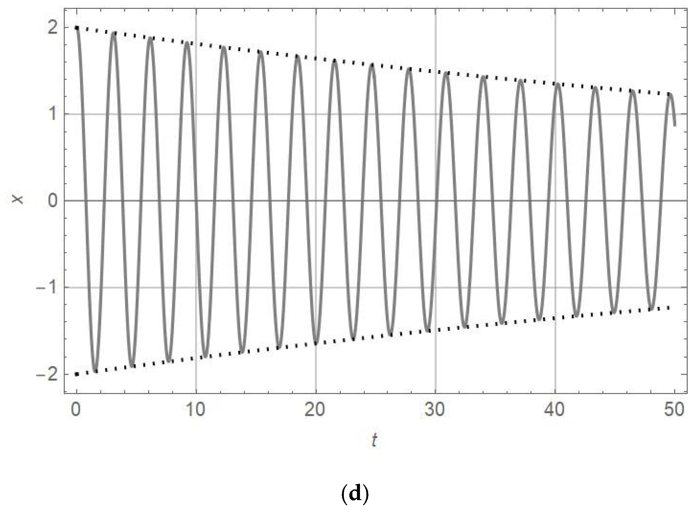
Example 2: Oscillators with Orders of Nonlinearity of α = 1.1; 3; and 7 and Various Damping Coefficients

To prove the accuracy of the analytically obtained results (52) and (53), three examples with different orders of nonlinearity and various values of damping coefficients are considered (see

Table 4. Models of oscillators for various α and ε values and the amplitude–time functions.

$\mathit{\alpha }$	$\mathit{\epsilon }$	Model of the Oscillator	${\mathit{A}}_{\mathit{a}}/{\mathit{A}}_0$
1.1	$0.10 c_1$	$\ddot{x}+c_{\alpha }^{2}x{\left|x\right|}^{0.1}+c_1^{2}x+2.1{0c}_1\dot{x}=0$	$\exp (-1.02439c_{1}t)$
	$0.25 c_1$	$\ddot{x}+c_{\alpha }^{2}x{\left|x\right|}^{0.1}+c_1^{2}x+2.25c_1\dot{x}=0$	$\exp (-1.09756c_{1}t)$
3	$-0.10 c_1$	$\ddot{x}+c_{\alpha }^{2}x{\left|x\right|}^2+c_1^{2}x+2.0\dot{c_{1}x}=0$	$\exp (-0.66666c_{1}t)$
	$0.40 c_1$	$\ddot{x}+c_{\alpha }^{2}x{\left|x\right|}^2+c_1^{2}x+2.5\dot{c_{1}x}=0$	$\exp (-0.83333c_{1}t)$
7	$-0.40 c_1$	$\ddot{x}+c_{\alpha }^{2}x{\left|x\right|}^6+c_1^{2}x+2.1c_1\dot{x}=0$	$\exp (-0.42000c_{1}t)$
	$0.10 c_1$	$\ddot{x}+c_{\alpha }^{2}x{\left|x\right|}^6+c_1^{2}x+2.6c_1\dot{x}=0$	$\exp (-0.52{000c}_{1}t)$

).

In Figure 4, Figure 5 and Figure 6, the numerically obtained x-t solutions of the differential equations given in Table 4 and the corresponding $A_a-t$ diagrams are plotted. The initial conditions are $x(0)=A_0, \dot{x}(0)=-\delta A_0=-A_0{c}_1\sqrt{2/(\alpha +1)}$. The parameter values are $c_1=0.01$, $c_{\alpha }=1$, and $A_0=1$.

In Figure 7, oscillators with linear and nonlinear coefficients $c_1=0.01, c_{\alpha }^2=1$, damping parameter $b=2.1$, and initial amplitude $A_0=1$, as well as various orders of nonlinearity ($\alpha =1.1, 3)$, are considered. For these parameter values, the numerically obtained $x-t$ and the approximately calculated $A_a-t$ diagrams are plotted.

Comparing the amplitudes and periods of vibration for oscillators of nonlinearity orders of $\alpha =1.1$, 3, and 7 with the damping parameter $b_e$ in Figure 1, Figure 2 and Figure 3 with those for $\left|b\right|=1.1 b_e$ plotted in Figure 4, Figure 5, Figure 6 and Figure 7, it is obtained that for $b>b_e$, the amplitude decrease is faster and the periods are longer. The analytically obtained solution $A_a/A_0$ is at the top of the numerically obtained solutions x-t of equations for motion, as presented in Table 4. This statement is valid for the damping coefficient in the interval $\left|b-b_e\right|\le 0.2$. The accuracy of the analytic solution is high if the perturbation of the damping coefficient is up to 20% around the exact value $b_e$.

5. Purely Nonlinear Damped Oscillators

The model of the pure nonlinear oscillator, i.e., the oscillator without a linear stiffness term ($c_1^2=0$), but with linear damping, is

$$\ddot{x}+c_{\alpha }^{2}x{\left|x\right|}^{\alpha -1}+b\dot{x}=0.$$

(52)

It has already been mentioned that there is no closed-form analytic solution for the damped pure cubic oscillator in terms of standard functions [33]. Using Abel’s equation of the second kind [2], it can be proven that this statement is valid for the pure oscillator of any order of nonlinearity (54) as well. Hence, in this paper, the approximate solution of (52) is derived using the exact Ateb solution of the undamped pure nonlinear oscillator (b = 0).

When multiplying (52) by $\dot{x}$ and integrating it over time, the energy equation is as follows:

$${\displaystyle \frac{{\dot{x}}^2}{2}}+c_{\alpha }^2{\displaystyle \frac{{⌊x⌋}^{\alpha +1}}{\alpha +1}}=E=const.,$$

(53)

where E is the constant energy of the oscillator. If we assume that the function x and its derivative $\dot{x}$ are in the form of cosine and sine Ateb functions [1], then

$$x=Aca(\alpha ,1,\mathsf{\Theta }), \dot{x}=-A\omega {\displaystyle \frac{2}{\alpha +1}}sa(1,\alpha ,\mathsf{\Theta }),$$

(54)

where A is the amplitude, $\mathsf{\Theta }(t)=\omega t+{\psi }_0$ is the total phase angle function, $\omega$ is the frequency, and ${\psi }_0$ is the phase shift of the Ateb function for the initial condition. After substituting (54) into (53), and using relation (4) and separating the terms with ${ca}^0$ and ${ca}^{\alpha +1}$, the unknown frequency is obtained:

$$\omega =A^{(\alpha -1)/2}\sqrt{{\displaystyle \frac{\alpha +1}{2}}{c}_{\alpha }^2},$$

(55)

The energy constant of the conservative oscillator is

$$E={\displaystyle \frac{1}{\alpha +1}}{c}_{\alpha }^2{A}^{\alpha +1}.$$

(56)

After restoring b to a non-zero value, the model of the oscillator (54) includes the damping term, which causes the energy variation according to

$${\displaystyle \frac{dE}{dt}}=-b{\dot{x}}^2.$$

(57)

To obtain the approximate solution of (59), the energy method [34], which was already developed for pure cubic oscillators, is adopted and modified into the procedure for solving damped pure nonlinear oscillators of any order of nonlinearity α. For the time-variable amplitude A(t) and time-variable phase function $\mathsf{\Theta }(t)=\int \omega (t)dt+{\psi }_0$, Equations (56), (55) and (54) are, respectively,

$$\begin{gathered} E(t)={\displaystyle \frac{1}{\alpha +1}}{c}_{\alpha }^2{A(t)}^{\alpha +1},\hspace{1em}\omega (t)={A(t)}^{(\alpha -1)/2}\sqrt{{\displaystyle \frac{\alpha +1}{2}}{c}_{\alpha }^2}, \\ \dot{x}=-A(t)\omega (t){\displaystyle \frac{2}{\alpha +1}}sa(1,\alpha ,\mathsf{\Theta }(t)). \end{gathered}$$

(58)

Substituting (58) into (57) yields

$${\displaystyle \frac{d}{dt}}\left({\displaystyle \frac{1}{\alpha +1}}{c}_{\alpha }^2{A(t)}^{\alpha +1}\right)=-b{\left(A(t)\omega (t){\displaystyle \frac{2}{\alpha +1}}sa(1,\alpha ,\mathsf{\Theta }(t))\right)}^2,$$

(59)

In other words,

$$\dot{A}(t)=-{\displaystyle \frac{2b}{\alpha +1}}{A(t)\left(sa(1,\alpha ,\mathsf{\Theta }(t))\right)}^2.$$

(60)

As the sa Ateb function has the period $2\mathsf{\Pi }=2B({\displaystyle \frac{1}{\alpha +1}},{\displaystyle \frac{1}{2}})$, where B is the beta function [32], it is at this point where the averaging of ${(sa(1,\alpha ,\mathsf{\Theta }))}^2$ over its period is carried out. The averaged value is $\underset{0}{\overset{2\mathsf{\Pi }}{\int }}{(s,(1.\alpha ,\mathsf{\Theta }))}^{2}d\mathsf{\Theta }={\displaystyle \frac{\alpha +1}{\alpha +3}}$ (see Equation (A13) in Appendix A). After integrating the averaged Equation (60) for the initial amplitude $A_0$, the approximate amplitude function is obtained:

$$A(t)=A_0\exp \left(-{\displaystyle \frac{2b}{\alpha +3}}t\right).$$

(61)

It is obvious that the amplitude depends on the damping coefficient b and the order of nonlinearity $\alpha$ and is independent of the coefficient of nonlinearity $c_{\alpha }^2$. These results correspond to relation (16) obtained for the damped strong nonlinear oscillator. After substituting (61) into (60), the approximate ω function is

$$\omega (t)=A_0^{{\displaystyle \frac{\alpha -1}{2}}}\sqrt{{\displaystyle \frac{\alpha +1}{2}}{c}_{\alpha }^2}\exp \left(-{\displaystyle \frac{b(\alpha -1)}{\alpha +3}}t\right).$$

(62)

Using (61) and (62), the approximate solution of (54) for the initial conditions $x(0)=A_0$ and $\dot{x}(0)=-A_0\delta =-{\displaystyle \frac{2b}{\alpha +3}}{A}_0$ is as follows:

$$x=A_0\mathrm{e}\mathrm{x}\mathrm{p}(-{\displaystyle \frac{2bt}{\alpha +3}})ca(\alpha ,1,{\displaystyle \frac{(\alpha +3)A_0^{\frac{\alpha -1}{2}}}{b(\alpha -1)}}\sqrt{c_{\alpha }^2{\displaystyle \frac{\alpha +1}{2}}}(1-\exp \left(-{\displaystyle \frac{b(\alpha -1)t}{\alpha +3}}\right)).$$

(63)

According to the procedure for period derivation, the time intervals $T_i$ are expressed with (21), where $i<2\omega /\mathsf{\Pi }$ and

$$\beta \delta ={\displaystyle \frac{b(\alpha -1)}{\alpha +3}},\hspace{1em}\hspace{1em}\omega ={\displaystyle \frac{(\alpha +3)A_0^{\frac{\alpha -1}{2}}}{b(\alpha -1)}}\sqrt{c_{\alpha }^2{\displaystyle \frac{\alpha +1}{2}}}.$$

(64)

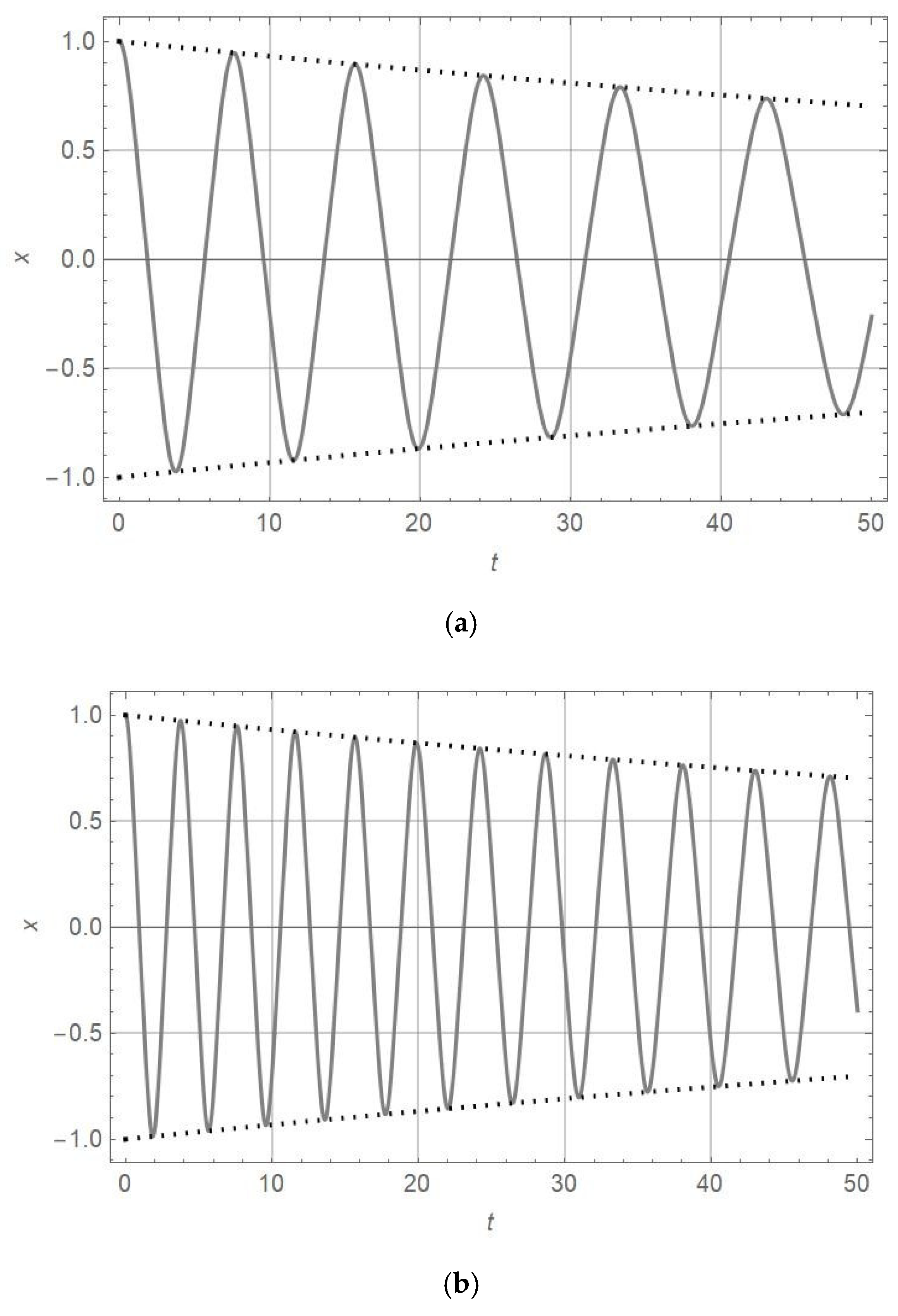
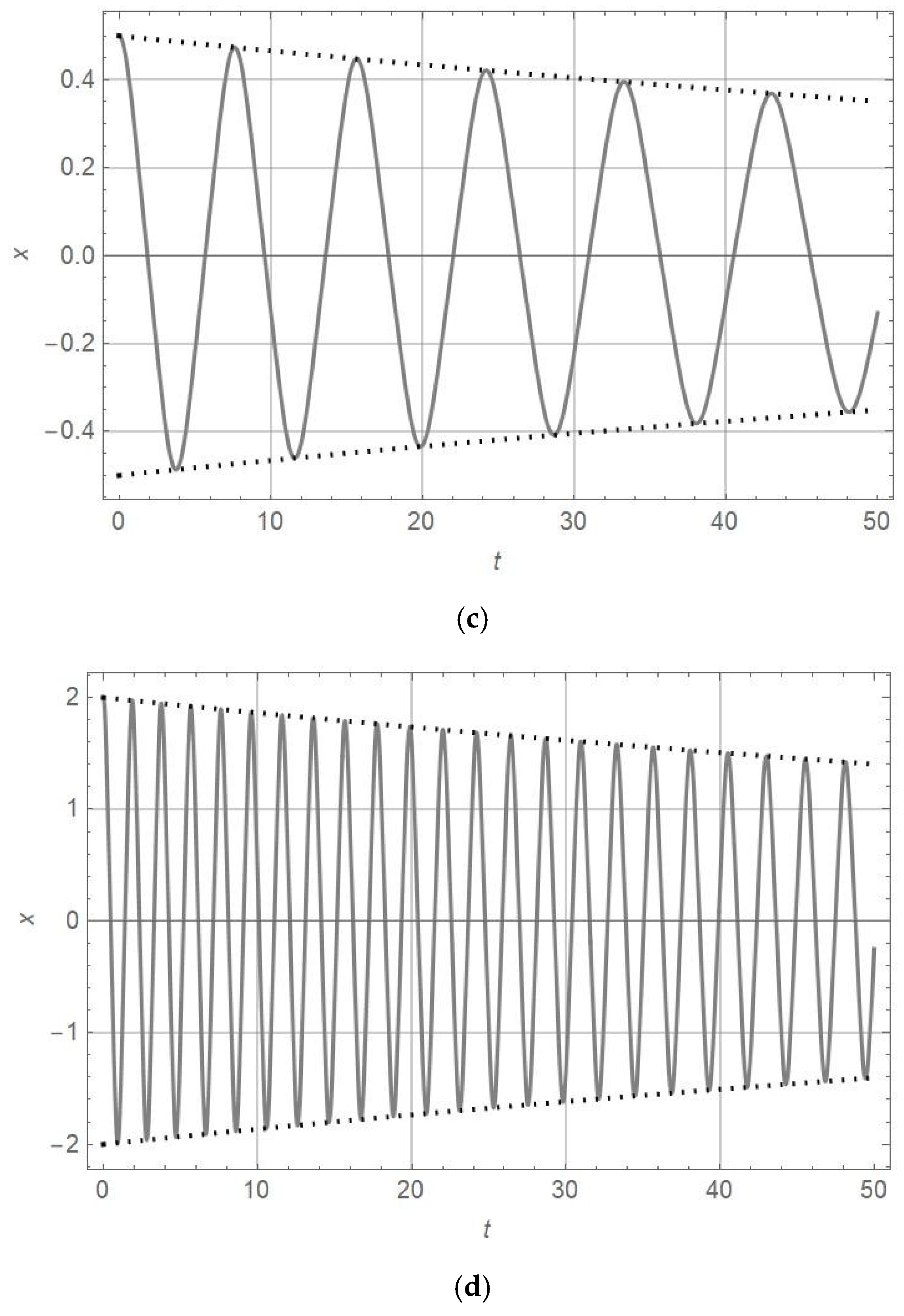
Example 3: Pure Cubic Oscillator with Linear Damping

For the oscillator with cubic nonlinearity and linear damping, where

$$\ddot{x}+c_{\alpha }^2{x}^3+b\dot{x}=0,$$

(65)

the approximate solution (65) for $\alpha =3$ is

$$x=A_0\exp \left(-{\displaystyle \frac{bt}{3}}\right)ca\left(\mathrm{3,1},{\displaystyle \frac{3A_0{c}_{\alpha }}{b}}\sqrt{2}\left(1-\exp \left(-{\displaystyle \frac{bt}{3}}\right)\right)\right).$$

(66)

Remark 5.

In [14], the approximate solution for the pure damped Duffing oscillator is obtained:

$$x=A_0\mathit{exp}\left(-{\displaystyle \frac{b}{3}}t\right)\mathit{cos}\left(-{\displaystyle \frac{3A_0{c}_3}{b}}{\displaystyle \frac{\sqrt{3}}{2}}\mathit{exp}\left(-{\displaystyle \frac{b}{3}}t\right)+C_0\right).$$

(67)

Comparing (66) and (67), it is obtained that the amplitude variation is equal, but the approximate periods of vibration differ.

According to (66), the amplitude–time variation is

$$A(t)=A_0\exp \left(-{\displaystyle \frac{b}{3}}t\right).$$

(68)

For $\beta \delta ={\displaystyle \frac{b}{3}}$, $\omega ={\displaystyle \frac{3}{b}}{A}_0\sqrt{2c_{\alpha }^2}$, and $\mathsf{\Pi }=5.2441$, expression (19) is

$$T_i={\displaystyle \frac{3}{b}}ln\left|{\displaystyle \frac{6A_0\sqrt{2c_{\alpha }^2}}{6A_0\sqrt{2c_{\alpha }^2}-5.2441bi}}\right|.$$

(69)

In

Table 5. Periods and amplitudes of vibration for the pure cubic nonlinear oscillator with linear damping.

	${\mathit{A}}_0 = 0.5$ $\mathit{b} = 0.1$ ${\mathit{c}}_{\mathit{\alpha }}^2 = 1$	${\mathit{A}}_0 = 1$ $\mathit{b} = 0.1$ ${\mathit{c}}_{\mathit{\alpha }}^2 = 1$	${\mathit{A}}_0 = 2$ $\mathit{b} = 0.1$ ${\mathit{c}}_{\mathit{\alpha }}^2 = 1$	${\mathit{A}}_0 = 1$ $\mathit{b} = {\mathit{b}}_{\mathit{e}} = 0.0212$ ${\mathit{c}}_{\mathit{\alpha }}^2 = 1$	${\mathit{A}}_0 = 1$ $\mathit{b} = 0.1$ ${\mathit{c}}_{\mathit{\alpha }}^2 = 2$
$T_0;A_0$	0.000; 0.500	0.000; 1.000	0.000; 2.000	0.000; 1.000	0.000; 1.000
$T_1;A_1$	3.971; 0.438	1.913; 0.938	0.942; 1.938	1.866; 0.987	1.340; 0.956
$T_2;A_2$	8.519; 0.376	3.958; 0.876	1.914; 1.876	3.757; 0.974	2.748; 0.912
$T_3;A_3$	13.90; 0.314	6.152; 0.814	2.918; 1.815	5.674; 0.961	4.216; 0.869
$T_4;A_4$	20.46; 0.253	8.519; 0.753	3.958; 1.753	7.617; 0.947	5.764; 0.825
$T_5;A_5$	28.872; 0.191	11.089; 0.691	5.035; 1.691	9.588; 0.934	7.396; 0.781
$T_6;A_6$	40.601; 0.129	13.900; 0.629	6.152; 1.629	11.586; 0.921	9.122; 0.738
$T_7;A_7$	60.126; 0.067	17.002; 0.567	7.312; 1.567	13.613; 0.908	10.054; 0.695
$T_8;A_8$	134.85; 0.005	20.461; 0.505	8.519; 1.505	15.669; 0.895	12.905; 0.650
$T_9;A_9$		24.374; 0.444	9.776; 1.444	17.775; 0.882	14.992; 0.607
$T_{10};A_{10}$		28.872; 0.382	11.089; 1.382	19.873; 0.869	17.235; 0.563
$T_{11};A_{11}$		34.176; 0.320	12.460; 1.320	22.023; 0.856	19.659; 0.519
$T_{12};A_{12}$		40.601; 0.258	13.900; 1.258	24.206; 0.843	22.206; 0.475
$T_I=T_4-T_0,$ $\Delta A_I=A_0-A_4$	20.46 0.247	8.519 0.247	3.958 0.247	7.617 0.053	5.764 0.175
$T_{II}=T_8-T_4,$ $\Delta A_{II}=A_4-A_8$	114.39 0.248	11.942 0.248	4.561 0.248	8.052 0.052	7.141 0.175
$T_{III}=T_{12}-T_8,$ $\Delta A_{III}=A_8-A_{12}$		20.141 0.247	5.381 0.247	8.537 0.052	9.301 0.175
${\displaystyle \frac{T_{II}-T_I}{T_I}}100\%$		40.181%	15.235%	5.71%	23.89%
${\displaystyle \frac{T_{III}-T_{II}}{T_{II}}}100\%$		68.657%	17.979%	6.02%	30.25%
${\displaystyle \frac{\Delta A_I}{A(T_0)}}100\%$	49.4%	24.7%	12.3%	5.3%	17.50%
${\displaystyle \frac{\Delta A_{II}}{A(T_4)}}100\%$	98.0%	32.9%	14.4%	5.49%	21.21%
${\displaystyle \frac{\Delta A_{III}}{A(T_8)}}100\%$		48.9%	16.4%	5.81%	26.92%

, data obtained by substituting various values of parameters b and $c_{\alpha }^2$ and initial amplitude $A_0$ into (68) and (69) are presented.

Analyzing the data in Table 5, the period of vibration is shorter for $c_{\alpha }^2=2$ than for $c_{\alpha }^2=1$. The local maxima of the amplitude are higher for $c_{\alpha }^2=2$ than for $c_{\alpha }^2=1.$ In addition, the period increase in time is faster for $c_{\alpha }^2=1$ than for $c_{\alpha }^2=2$. The amplitude decay to zero is the fastest for $A_0=0.5$ and the slowest for $A_0=2.$ The period of vibration is the longest for $A_0=0.5,$ shorter for $A_0=1$, and the shortest for $A_0=2$.

For the purely nonlinear oscillator, the period of vibration is shorter for higher values of $c_{\alpha }^2$. The local maximum in the x-t diagrams is higher for $c_{\alpha }^2$ than for smaller values. The period increase in time is faster for smaller values of $c_{\alpha }^2$ than for higher values.

Comparing the data for the Duffing oscillator in Table 2 and for the pure cubic oscillator in Table 5, the difference in amplitude and period of vibration is discussed. The oscillators have the same initial amplitudes and parameters, including the damping coefficient. It is obvious that, for both oscillators, the amplitude–time functions are equal. The periods of vibration are longer for pure cubic oscillators than for the Duffing one. Thus, the local maxima in cubic oscillators are lower than those in the Duffing oscillator. In addition, the period increase in time is faster in the cubic oscillator than in the Duffing oscillator. The linear term of the elastic force causes higher frequencies of vibration. Finally, it has to be mentioned that the difference is quite small and is up to 1%.

6. Discussion

The results presented in this study offer a comprehensive insight into the dynamic behavior of damped nonlinear oscillators of arbitrary order, particularly those for which an exact analytical solution exists under a specific relation between the damping and stiffness coefficients. The derived condition (10) serves as a critical threshold that guarantees the integrability of the governing equation, where $\alpha \in \mathbb{R}$, $\alpha \ge 1$, defines the order of nonlinearity. One of the key findings is that the amplitude of oscillation decreases over time and that this decay is governed by the initial amplitude, the damping coefficient, and the nonlinear exponent α\alphaα, while it remains independent of the stiffness coefficient $c_1^2$. This suggests a decoupling between the stiffness-related restoring force and the dissipative mechanism in terms of amplitude evolution. Notably, the amplitude damping is the fastest in the linear case ($\alpha =1$) and becomes progressively slower with increasing nonlinearity. In the limiting case, as $\alpha \to \infty$, the amplitude approaches a constant value, indicating a near-isochronous and persistent oscillatory regime for strongly nonlinear systems. The time dependence of the vibration period further distinguishes nonlinear damped oscillators from their linear counterparts. While the period remains constant in linear systems, it increases over time in nonlinear systems, with the rate of increase being greater for higher values of $\alpha$. This implies that nonlinearities not only slow the amplitude decay but also introduce a nontrivial modulation of the temporal characteristics of oscillation.

An important analytical tool in this study is the first integral of the motion, which facilitates the derivation of exact solutions and provides a method for determining initial phase and amplitude from initial conditions. This integral proves to be particularly useful in constructing both exact and approximate solutions and highlights the role of conserved quantities in systems with specific parameter constraints.

When the damping coefficient deviates moderately (up to approximately 20%) from the critical value b_e, the proposed approximate solution—a perturbation of the exact one—remains highly accurate. This robustness enhances the practical utility of the method for modeling real-world systems where parameter uncertainty is inevitable.

In contrast, for purely nonlinear damped oscillators (i.e., systems without a linear stiffness term), an exact analytic solution is not attainable even in terms of the Ateb function. Nevertheless, an approximate solution based on the undamped case—incorporating time-varying amplitude and phase—has been shown to effectively describe system behavior. This is particularly useful for small initial amplitudes, where damping effects are more pronounced, leading to faster amplitude decay and longer vibration periods.

A particularly interesting observation is the equivalence of amplitude–time functions for the purely nonlinear damped oscillator and the strongly nonlinear oscillator with linear damping, provided that both systems share the same damping coefficient, order of nonlinearity, and initial amplitude. This suggests a deeper structural similarity in the energy dissipation mechanisms of the two systems, despite differences in their formulation.

Overall, these findings contribute to the broader understanding of nonlinear dynamical systems and offer a unified framework for analyzing damped oscillators across a continuous spectrum of nonlinearities. The analytical and approximate methods developed here lay the foundation for future work on systems with more complex damping models, such as nonlinear or hysteretic damping.

7. Conclusions

The following is concluded:

• The strong nonlinear oscillator with linear damping has the exact solution for $b_e/c_1=(\alpha +3)/\sqrt{2(\alpha +1)}$, where $b_e$ is the damping coefficient, $c_1^2$ is the coefficient of linear stiffness, and $\alpha \ge 1$ and $\alpha \in \mathbb{R}$ are the orders of the equation’s nonlinearity (an integer or non-integer).
• The motion of the strong nonlinear oscillator with linear damping is influenced by time-decaying amplitudes and also by time-variable periods.
• The amplitude time decrease is the function of the initial amplitude, the damping coefficient, and the order of nonlinearity, but it is independent of the coefficient of stiffness. The amplitude damping is the fastest for the linear oscillator and is slower for oscillators with higher orders of nonlinearity. If the order of nonlinearity tends to infinity, then the amplitude tends to the constant initial amplitude. In addition, independently of the order of nonlinearity, the amplitude decay is faster for higher damping coefficients and smaller initial amplitudes.
• The vibration varies with increasing time periods. The period increase is faster for oscillators with a higher order of nonlinearity and is zero for the linear damped oscillator. When comparing the first periods of vibration for damped oscillators with various orders of nonlinearity, it is obtained that the period of vibration is longer for higher orders of nonlinearity than for lower ones.
• The first integral for the nonlinear oscillator with linear damping and certain parameter values is determined. The first integral is available for the derivation of the exact solution. Using the integral, the initial amplitude and phase shift for the initial deflection and velocity are obtained.
• The approximate solution, which is the perturbed version of the exact solution, is the appropriate one for oscillators with damping coefficient variations up to 20%.
• The damped pure nonlinear oscillator has no exact solution even in the form of the Ateb function. The approximate solution, based on the exact solution of the undamped oscillator, is convenient for application.
• In the damped pure nonlinear oscillator with small initial amplitudes, the amplitude decay is faster, and the period of vibration is longer with a greater tendency to increase compared to the oscillator with a higher initial amplitude.
• The amplitude–time function for the damped pure nonlinear oscillator and for the strong nonlinear oscillator is equal if both oscillators have the same order of nonlinearity, damping coefficient, and initial amplitudes of vibration.

Further research should be conducted on the vibration analysis of oscillators with any order of nonlinear damping.

References

1. Cveticanin, L. Strong Nonlinear Oscillators—Analytical Solutions, 2nd ed.; Mathematical Engineering; Springer: Berlin/Heidelberg, Germany, 2018. [Google Scholar]
2. Panayotounakanos, D.E.; Panayotounakou, N.D.; Vakakis, A.V. On the solution of the unforced damped Duffing oscillator with no linear stiffness term. Nonlinear Dyn. 2002, 28, 1–16. [Google Scholar] [CrossRef]
3. Bakhtiari-Nejad, F.; Nazari, M. Nonlinear vibration analysis of isotropic cantilever plate with viscoelastic laminate. Nonlinear Dyn. 2009, 56, 325–356. [Google Scholar] [CrossRef]
4. Wang, Y.R.; Feng, C.K.; Chen, S.Y. Damping effects of linear and nonlinear tuned mass dampers on nonlinear hinged-hinged beam. J. Sound Vib. 2018, 430, 150–173. [Google Scholar] [CrossRef]
5. Baumann, B.; Schwieger, J.; Wol, M.; Manders, F.; Suijker, J. Nonlinear behavior in high-intensity discharge lamps. J. Phys. D Appl. Phys. 2015, 49, 255201. [Google Scholar] [CrossRef]
6. Salas, A.H.; El-Tantawy, S.A. On the approximate solutions to a damped harmonic oscillator with higher-order nonlinearities and its application to plasma physics: Semi-analytical solution and moving boundary method. Eur. Phys. J. Plus 2020, 135, 833–917. [Google Scholar] [CrossRef]
7. Hammad, A.M.; Salas, A.H.; El-Tantawy, S.A. New method for solving strong conservative odd parity nonlinear oscillators: Applications to plasma physics and rigid rotator. AIP Adv. 2020, 10, 085001. [Google Scholar] [CrossRef]
8. Younesian, D.; Askari, H.; Saadatania, Z.; Yazdi, M.K. Periodic solutions for nonlinear oscillation of a centrifugal governor system using the He’s frequency–amplitude formulation and He’s energy balance method. Nonlinear Sci. Lett. A 2011, 2, 143–148. [Google Scholar]
9. Salas, A.H.; El-Tantawy, S.A. Analytical solutions of some strong nonlinear oscillators. In Engineering Problems—Uncertainties, Constraints and Optimization Techniques; Tsuzuki, M.S.G., Takimoto, R.Y., Sato, A.K., Saka, T., Barari, A., Rahman, R.O.A., Hung, Y.-T., Eds.; IntechOpen: London, UK, 2019; 25p. [Google Scholar] [CrossRef]
10. Kontomaris, S.V.; Mazi, I.; Chiliveros, G.; Malamou, A. Generic numerical and analytical methods for solving nonlinear oscillators. Phys. Scr. 2024, 99, 02523. [Google Scholar] [CrossRef]
11. El-Shahed, M. Application of differential transform method to non-linear oscillatory systems. Commun. Nonlinear Sci. Numer. Simul. 2008, 13, 1714–1720. [Google Scholar] [CrossRef]
12. Nourazar, S.; Mirzabeigy, A. Approximate solution for nonlinear Duffing oscillator with damping effect using the modified differential transform method. Sci. Iran. B 2013, 20, 364–368. [Google Scholar]
13. Abdeljhafez, H.M. Solution of excited non-linear oscillators under damping effects using the modified differential transform method. Mathematics 2016, 4, 11. [Google Scholar] [CrossRef]
14. Wu, B.S.; Sun, W.P. Construction of approximate analytical solutions to strongly nonlinear damped oscillators. Arch. Appl. Mech. 2011, 81, 1017–1030. [Google Scholar] [CrossRef]
15. Razzak, M.A. An analytical approximate technique for solving cubic–quintic Duffing oscillator. Alex. Eng. J. 2016, 55, 2959–2965. [Google Scholar] [CrossRef]
16. Mandal, S. Classical damped quartic anharmonic oscillator a simple analytical approach. Int. J. Non-Linear Mech. 2003, 38, 1095–1101. [Google Scholar] [CrossRef]
17. Turkyilmazoglu, M. An effective approach for approximate analytical solutions of the damped Duffing equation. Phys. Scr. 2012, 86, 015301. [Google Scholar] [CrossRef]
18. Cveticanin, L. Homotopy-perturbation method for pure non-linear differential equation. Chaos Solitons Fractals 2006, 30, 1221–1230. [Google Scholar] [CrossRef]
19. Cveticanin, L. Oscillators with nonlinear elastic and damping forces. Comp. Math. Appl. 2011, 62, 1745–1757. [Google Scholar] [CrossRef]
20. Jojannessen, K. The Duffing oscillator with damping. Eur. J. Phys. 2015, 36, 065020. [Google Scholar] [CrossRef]
21. Johannessen, K. The Duffing oscillator with damping for a softening potential. Int. J. Appl. Comput. Math. 2017, 3, 3805–3816. [Google Scholar] [CrossRef]
22. Johannessen, K. The solution to the differential equation with linear damping describing a physical systems governed by a cubic energy potential. arXiv 2018. [Google Scholar] [CrossRef]
23. Cveticanin, L. On the truly nonlinear oscillator with positive and negative damping. Appl. Math. Comput. 2014, 243, 433–445. [Google Scholar] [CrossRef]
24. Cveticanin, L.; Herisanu, N.; Ismail, G.M.; Zukovic, M. Vibration of the Liénard oscillator with quadratic damping and constant excitation. Mathematics 2025, 13, 937. [Google Scholar] [CrossRef]
25. Panayotounakos, D.E.; Theotokoglou, E.E.; Markakis, M.P. Exact analytic solutions for the damped Duffing nonlinear oscillator. Comptes Rendus Méc. 2006, 334, 311–316. [Google Scholar] [CrossRef]
26. Elias-Zuniga, A. Analytical solution of the damped Helmholtz–Duffing equation. Appl. Math. Lett. 2012, 25, 2349–2353. [Google Scholar] [CrossRef]
27. Salas, A.H.; El-Tantawy, S.A.; Castillo, J.H. Analytical solution to the damped cubic-quintic Duffing equation. Int. J. Math. Comput. Sci. 2022, 17, 425–430. [Google Scholar]
28. Almendrai, J.A.; Sanjuan, M.A.F. Integrability and symmetries for the Helmholtz oscillator with friction. J. Phys. A Math. Gen. 2003, 36, 695–710. [Google Scholar] [CrossRef]
29. Zhu, J.-W. A new exact solution of a damped quadratic nonlinear oscillator. Appl. Math. Model. 2014, 38, 5986–5993. [Google Scholar] [CrossRef]
30. Salas, A.H.; El-Tantawy, S.A.; Aljahdaly, N.H. An exact solution to the quadratic damping strong nonlinearity Duffing oscillator. Math. Probl. Eng. 2021, 15, 8875589. [Google Scholar] [CrossRef]
31. Cveticanin, L.; Vujkov, S.; Cveticanin, D. Application of Ateb and Generalized trigonometric functions for nonlinear oscillators. Arch. Appl. Mech. 2020, 90, 2579–2587. [Google Scholar] [CrossRef]
32. Gradsein, I.S.; Rjizhik, I.M. Table of Integrals, Series and Products; Academic Press: Moscow, Russia, 1971. (In Russian) [Google Scholar]
33. Euler, N.; Steeb, W.-H.; Cyryus, K. On exact solutions for damped anharmonic oscillators. J. Phys. A Math. Gen. 1989, 22, L195–L199. [Google Scholar] [CrossRef]
34. Koscielniak, S.R. Weakly Damped Anharmonic Oscillator; TRIUMF Beam Note TRI-BN-24–21; TRIUMF: Vancouver, BC, Canada, 2015. [Google Scholar]
35. Rosenberg, R.M. The Ateb(h)-functions and their properties. Q. Appl. Math. 1963, 21, 37–47. [Google Scholar] [CrossRef]
36. Senik, P.M. Inversions of the incomplete beta function. Ukr. Math. J. 1969, 21, 271–278. [Google Scholar] [CrossRef]
37. Cveticanin, L.; Zukovic, M.; Cveticanin, D. Approximate analytic frequency of strong nonlinear oscillator. Mathematics 2024, 12, 3040. [Google Scholar] [CrossRef]
Figure 1. x t diagram (full line) and A a t diagram (dotted line) for α = 1.1 , c 1 = 0.01 and (a) c α = 1 , A 0 = 1 ; (b) c α = 2 , A 0 = 1 ; (c) c α = 2 , A 0 = 0.5 ; and (d) c α = 2 , A 0 = 2 .
Mathematics 13 01662 g001aMathematics 13 01662 g001b
Figure 2. x t diagram (full line) and A a t diagram (dotted line) for α = 3 , c 1 = 0.01 and (a) c α = 1 , A 0 = 1 ; (b) c α = 2 , A 0 = 1 ; (c) c α = 2 , A 0 = 0.5 ; and (d) c α = 2 , A 0 = 2 .
Mathematics 13 01662 g002aMathematics 13 01662 g002b
Figure 3. x t diagram (full line) and A a t diagram (dotted line) for α = 7 , c 1 = 0.01 and (a) c α = 1 , A 0 = 1 ; (b) c α = 2 , A 0 = 1 ; (c) c α = 2 , A 0 = 0.5 ; and (d) c α = 2 , A 0 = 2 .
Mathematics 13 01662 g003aMathematics 13 01662 g003b
Figure 4. x t diagram (full line) and A a t diagram (dotted line) for α = 1.1 , c 1 = 0.01 , c α = 1 , and A 0 = 1 , as well as for (a) ε = 0.1   c 1 and (b) ε = 0.25   c 1 .
Mathematics 13 01662 g004
Figure 5. x t diagram (full line) and A a t diagram (dotted line) for α = 3 , c 1 = 0.01 , c α = 1 , and A 0 = 1 , as well as for (a )   ε = 0.1   c 1 and (b) ε = 0.4   c 1 .
Mathematics 13 01662 g005
Figure 6. x t diagram (full line) and A a t diagram (dotted line) for α = 7 , c 1 = 0.01 , c α = 1 , and A 0 = 1 , as well as for (a )   ε = 0.1   c 1 and (b) ε = 0.1   c 1 .
Mathematics 13 01662 g006aMathematics 13 01662 g006b
Figure 7. x t diagram (full line) and A a t diagram (dotted line) for c 1 = 0.01 , c α = 1 , A 0 = 1 , and b = 2.1   c 1 and various orders of nonlinearity: (a) α = 1.1 ; (b) α = 3 .
Mathematics 13 01662 g007