A Graphical Suprametric Approach to Dynamic Market Structures

Abstract

This study presents a concise analytical framework that combines suprametric spaces with directed graph structures to model dynamic market environments. The proposed setting captures hierarchical and asymmetric relations between economic components, providing a more flexible structure than conventional metric frameworks. Within this framework, several types of contractive mappings, such as supra-Kannan, supra-Reich, and supra-Ciric contractions, are defined, and corresponding fixed point theorems are established. The theoretical results are applied to a nonlinear integral equation describing the evolution of prices in production and consumption processes. Under appropriate assumptions, the existence and uniqueness of solutions are guaranteed, and a numerical example demonstrates the convergence and practical importance of the proposed model.

1. Introduction and Preliminaries

The fundamental work of S. Banach [1] introduced a new branch of mathematics, now widely recognized as fixed point theory. Following this pivotal development, S. Saks [2] significantly contributed by introducing innovative approaches to multivalued mappings and exploring the topological characteristics of fixed points. This succession of groundbreaking research has culminated in the development of a comprehensive framework that builds upon Banach’s initial findings and stimulates a wide range of research initiatives. Moreover, it has enabled various practical applications in the field of fixed point theory, highlighting its significance and versatility.

Recently, Samuel et al. [3] and Rajkumar et al. [4] employed their fixed point findings to address fractional integral equations essential for modeling in mathematical modeling and applied sciences. In a similar manner, Ramaswamy et al. [5] developed the concept of fixed points to the boundary value problems and showed that they are useful in generalized contraction conditions when considering the best proximity point. Gnanaprakasam et al. [6] also extended new contraction mappings to Fredholm and integro-differential equations, which demonstrates the ability of fixed point results in a functional analysis. Moreover, Moussaoui [7] added a broader view covering fuzzy and admissibility frameworks to f-weak contractions due to the flexibility of fixed point methods in dealing with nonlinear and uncertain systems.

The study of fixed point theory and its practical applications involves a range of research considerations based on contractions, metric spaces with graphs, ordered metric spaces, modular function spaces, and so on (see [8,9,10,11]). In 2007, Jachymski [12] delved into the concept of contractions in graph spaces, establishing meaningful connections between these areas. Following this, Nieto et al. [13] explored fixed point theorems in ordered spaces that year, shedding light on the relationship between order theory and fixed point theory. Expanding on these findings, O’Regan et al. [14] further developed the theory in 2008 by extending contraction conditions to ordered spaces.

Inspired by these developments, Beg and Butt [15] studied set-valued graph contraction mappings, generalizing fixed point theorems via functional relations. Alfuraidan [16] later integrated modular function spaces with fixed point theory, examining the existence of fixed points for multivalued mappings with closed graphs in modular topological spaces. In 2017, Mirmostafaee et al. [17] extended coupled fixed point results by studying mappings on b-metric spaces endowed with graph structures. The same year, Shukla [18] introduced a comprehensive framework for fixed point theory within the graphical structure of metric spaces, unifying classical fixed point results under a single approach. In 2019, Chuensupantharat [19] investigated graphical b-metric spaces, highlighting the practical utility of graphic contraction mappings. Additionally, Younis et al. contributed to the field by demonstrating diverse applications of graphical fixed points through various graph-based metric structures, as detailed in their works [20,21,22].

Throughout this work, $\mathbb{R}$ will denote the set of all real numbers, ${\mathbb{R}}_{+}$ will stand for the set of non-negative real numbers, and $\mathbb{N}$ will represent the set of positive integers.

To establish the groundwork for our discussion, we first present some essential concepts and definitions that will play a pivotal role in the analysis that follows.

In 2008, Jachymski [12] described a construction, where ∐ is a nonempty set and $\Delta$ is the diagonal of $\coprod \times \coprod$. He defined a directed graph $\mathcal{G}=\left(\mathbb{V}\right(\mathcal{G}),\Xi (\mathcal{G}\left)\right)$ free from parallel edges, where $\mathbb{V}\left(\mathcal{G}\right)$ is the vertex set of $\mathcal{G}$, aligning with the set ∐, and $\mathbb{E}\left(\mathcal{G}\right)$ is the edge set of $\mathcal{G}$, including all the loops of $\mathcal{G}$, such that $\Delta \subseteq \Xi \left(\mathcal{G}\right)$. The graph ${\mathcal{G}}^{-1}$ is gained by reversing the trajectory of $\Xi \left(\mathcal{G}\right)$. If $\mathcal{G}$ owns symmetric edges is identified as $\breve{\mathcal{G}}$, in such a way that

$$\Xi \left(\breve{\mathcal{G}}\right)=\Xi \left({\mathcal{G}}^{-1}\right)\cup \Xi \left(\mathcal{G}\right).$$

Assume that $\sout{\partial }$ and $\vartheta$ are vertices in the directed graph $\mathcal{G}$. A path in $\mathcal{G}$ is a sequence ${\left\{{\sout{\partial }}_{\rho }\right\}}_{\rho =0}^m$ of $(m+1)$ vertices, whereby ${\sout{\partial }}_0=\sout{\partial }$, ${\sout{\partial }}_m=\vartheta$ accompanied by $({\sout{\partial }}_{\rho -1},{\sout{\partial }}_{\rho })\in \Xi \left(\mathcal{G}\right)$, where $\rho =1,2,\dots ,m$. A graph $\mathcal{G},$ is referred to as connected when a group of edges can connect any two vertices. An undirected graph $\mathcal{G}$ is weakly connected if a sequence of edges can join any two vertices within it. A graph $\psi =\left(\mathbb{V}\left(\mathcal{G}\right),\Xi \left(\mathcal{G}\right)\right)$ is a subgraph of $\psi =\left(\mathbb{V}\right(\mathcal{G}),\Xi (\mathcal{G}\left)\right)$ if all the vertices $\mathbb{V}\left(\mathcal{G}\right)\subseteq \mathbb{V}\left(\mathcal{G}\right)$ and all the edges $\Xi \left(\mathcal{G}\right)\subseteq \Xi \left(\mathcal{G}\right)$ meet these requirements in the same order.

In 2017, Shukla [18] presented the notion that $[\sout{\partial }{]}_{\mathcal{G}}^l$={$\vartheta$$\in \coprod :$ A directed path from $\sout{\partial }$ to $\vartheta$ in $\mathcal{G}$ having length $l\}.$ A relation $\mathcal{P}$ on ∐ to such an extent that ${\left(\sout{\partial }\mathcal{P}\vartheta \right)}_{\mathcal{G}}$ signifies a way from $\sout{\partial }$ to $\vartheta$ in $\mathcal{G}$ suggests that in the path that $\varpi \in (\sout{\partial }\mathcal{P}$$\vartheta$), $\varpi$ lies on the way ${\left(\sout{\partial }\mathcal{P}\vartheta \right)}_{\mathcal{G}}$. Moreover, a sequence ${\left\{{\sout{\partial }}_{\nu }\right\}}_{\nu \in \mathbb{N}}\subset \coprod$ is supposed to be $\mathcal{G}$−termwise connected ($\mathcal{G}$$-\mathcal{AWC}$) if ${\left({\sout{\partial }}_{\nu }\mathcal{P}{\sout{\partial }}_{\nu +1}\right)}_{\mathcal{G}}$ for all $\nu \in \mathbb{N}$. From this point forward, all graphs are considered as directed unless otherwise stated.

In 2022, Berzig [23] established a novel framework known as a suprametric space, which alters the conventional triangle inequality and investigates several fundamental properties of its associated topology. Subsequently, Panda et al. [24] advanced the discourse by defining extended suprametric spaces and formulating the contraction principle through elementary properties of the greatest lower bound, without using the ordinary iteration method. Furthermore, Panda et al. [25] expanded the research landscape by presenting the concept of graphically extended suprametric spaces and defining supra-graphical contractive mappings within these frameworks. For a thorough exploration of the studies related to suprametric concepts, it is essential to consult [26,27,28,29,30], which provide critical insights and foundational perspectives on the topic.

This paper further develops the analytical structure of graphically extended suprametric spaces by formulating new classes of contractive mappings namely supra-Kannan, supra-Reich, and supra-Ciric types and establishing corresponding fixed point theorems within this generalized framework. These results significantly broaden the applicability of classical contraction principles to settings characterized by direction-dependent and hierarchical relationships. In addition to its theoretical advancements, the study introduces an application oriented perspective by employing the proposed framework to analyze a dynamic market system represented through a nonlinear integral equation. This dual contribution, combining rigorous mathematical formulation with an interpretable economic context, underscores the potential of graph-based suprametric analysis as a versatile tool for modeling complex interactive influence.

Definition 1

([25]). Assume that ∐ is a nonempty set equipped with a graph  $\mathcal{G}.$ Consider the function $E_s^{\mathcal{G}}:\coprod \times \coprod \to \mathbb{R}$, which provides to the subsequent featured properties

$\left(i\right)$

$E_s^{\mathcal{G}}(\sout{\partial },\vartheta )\ge 0,$ for all $\sout{\partial },\vartheta \in \coprod ;$

$\left(ii\right)$

$E_s^{\mathcal{G}}\left(\sout{\partial },\vartheta \right)=0$ if and only if $\sout{\partial }=\vartheta ;$

$\left(iii\right)$

$E_s^{\mathcal{G}}(\sout{\partial },\vartheta )=E_s^{\mathcal{G}}(\vartheta ,\sout{\partial }),$ for all $\sout{\partial },\vartheta \in \coprod ;$

$\left(iv\right)$

there exists a function $\psi :\coprod \times \coprod \to \left[1,\infty \right)$ and for all $\sout{\partial },\vartheta ,z\in \coprod$ such that ${\left(\sout{\partial }\mathcal{P}\vartheta \right)}_{\mathcal{G}},$$z\in {\left(\sout{\partial }\mathcal{P}\vartheta \right)}_{\mathcal{G}}$ which implies

$$E_s^{\mathcal{G}}\left(\sout{\partial },\vartheta \right)\le E_s^{\mathcal{G}}\left(\sout{\partial },z\right)+E_s^{\mathcal{G}}\left(z,\vartheta \right)+\psi \left(\sout{\partial },\vartheta \right)E_s^{\mathcal{G}}\left(\sout{\partial },z\right)E_s^{\mathcal{G}}\left(z,\vartheta \right),$$

then, the pair $(\coprod ,E_s^{\mathcal{G}})$ is referred to as a graphically extended suprametric space equipped with the graph $\mathcal{G}$.

Remark 1.

• The control function $\psi (\sout{\partial },\vartheta )$ has both analytical and geometric significance. Analytically, it provides a controlled relaxation of the standard triangle inequality, allowing the framework to incorporate small perturbations or nonlinear distortions arising in complex networks. Geometrically, $\Psi (\sout{\partial },\vartheta )$ can be interpreted as a local deviation factor that measures how far the indirect path $\sout{\partial }\to z\to \vartheta$ deviates from the direct connection $\sout{\partial }\to \vartheta$ in the graphical structure. When $\psi (\sout{\partial },\vartheta )=k\ge 0$, the framework reduces to the classical suprametric case, whereas a bounded positive ψ represents a controlled curvature or interaction intensity between the nodes of the graph.
• It’s vital to take note that not all graphically extended suprametric spaces are extended suprametric spaces.

In the context of an extended graphical suprametric space $(\coprod ,E_s^{\mathcal{G}})$, consider a point $\sout{\partial }\in \coprod$ and a positive real number $\epsilon$. The definitions of $E_s^{\mathcal{G}}-$open ball and $E_s^{\mathcal{G}}-$closed ball, both centered at the point ${\sout{\partial }}_0$ and with radius $\epsilon$ are described as

• ${\mathbb{B}}_{E_s^{\mathcal{G}}}\left(\sout{\partial },\epsilon \right)=\left\{\left.\vartheta \in \coprod \right|{\left(\sout{\partial }\mathcal{P}\vartheta \right)}_{\mathcal{G}},E_s^{\mathcal{G}}\left(\sout{\partial },\vartheta \right)<\epsilon \right\}$,
• ${\overline{\mathbb{B}}}_{E_s^{\mathcal{G}}}\left(\sout{\partial },\epsilon \right)=\left\{\left.\vartheta \in \coprod \right|{\left(\sout{\partial }\mathcal{P}\vartheta \right)}_{\mathcal{G}},E_s^{\mathcal{G}}\left(\sout{\partial },\vartheta \right)\le \epsilon \right\}$.

As $\Delta \subseteq \Xi \left(\mathcal{G}\right)$, this clearly indicates that $\sout{\partial }\in {\mathbb{B}}_{E_s^{\mathcal{G}}}\left(\sout{\partial },\epsilon \right)$ and hence, ${\mathbb{B}}_{E_s^{\mathcal{G}}}\left(\sout{\partial },\epsilon \right)\ne \varnothing$ for all $\sout{\partial }\in \coprod$ and $\epsilon >0$. In addition, a neighborhood system is constructed represented by the collection $\mathcal{B}=\left\{\left.E_s^{\mathcal{G}}\left(\sout{\partial },\epsilon \right)\right|\sout{\partial }\in \coprod ,\epsilon >0\right\}$. This set effectively captures the relationships within the space by incorporating all points $\sout{\partial }$ in ∐ alongside their respective positive radii $\epsilon$.

Remark 2.

The definition of the $E_s^{\mathcal{G}}-$open and $E_s^{\mathcal{G}}-$closed balls relies on the fact that the extended suprametric function $E_s^{\mathcal{G}}:\mathbb{V}\left(\mathcal{G}\right)\times \mathbb{V}\left(\mathcal{G}\right)\to [0,\infty )$ is defined for all vertex pairs in the directed graph $\mathcal{G}$, together with the existence of a reachability relation ${\left(\sout{\partial }\mathcal{P}\vartheta \right)}_{\mathcal{G}}$ which ensures path connectivity. Formally, for any $\sout{\partial }\in \mathbb{V}\left(\mathcal{G}\right)$ and $\epsilon >0$, the $E_s^{\mathcal{G}}$–open ball is defined by

$${\mathbb{B}}_{E_s^{\mathcal{G}}}(\sout{\partial },\epsilon )=\{\vartheta \in \mathbb{V}\left(\mathcal{G}\right)\mid {\left(\sout{\partial }\mathcal{P}\vartheta \right)}_{\mathcal{G}},E_s^{\mathcal{G}}(\sout{\partial },\vartheta )<\epsilon \}\ne \varnothing .$$

Since the diagonal $\Delta =\left\{\right(\sout{\partial },\sout{\partial })\mid \sout{\partial }\in \mathbb{V}(\mathcal{G}\left)\right\}$ is contained in $\Xi \left(\mathcal{G}\right)$, every vertex $\sout{\partial }$ satisfies ${\left(\sout{\partial }\mathcal{P}\sout{\partial }\right)}_{\mathcal{G}}$ and $E_s^{\mathcal{G}}(\sout{\partial },\sout{\partial })=0<\epsilon$, which implies $\sout{\partial }\in {\mathbb{B}}_{E_s^{\mathcal{G}}}(\sout{\partial },\epsilon )$ and consequently ${\mathbb{B}}_{E_s^{\mathcal{G}}}(\sout{\partial },\epsilon )\ne ⌀$ for all $\epsilon >0$. This guarantees that each vertex possesses a non-empty neighborhood.

Furthermore, the family of all such balls

$$\mathcal{B}=\{{\mathbb{B}}_{E_s^{\mathcal{G}}}(\sout{\partial },\epsilon )\mid \sout{\partial }\in \mathbb{V}\left(\mathcal{G}\right),\epsilon >0\}$$

satisfies the neighborhood axioms:

$\left(i\right)$

For every $\sout{\partial }\in \mathbb{V}\left(\mathcal{G}\right)$ and open set U containing $\sout{\partial }$, there exists $\epsilon >0$ with ${\mathbb{B}}_{E_s^{\mathcal{G}}}(\sout{\partial },\epsilon )\subseteq U$;

$\left(ii\right)$

If $\vartheta \in {\mathbb{B}}_{E_s^{\mathcal{G}}}(\sout{\partial },\epsilon )$, then there exists $\delta >0$ such that ${\mathbb{B}}_{E_s^{\mathcal{G}}}(\vartheta ,\delta )\subseteq {\mathbb{B}}_{E_s^{\mathcal{G}}}(\sout{\partial },\epsilon )$.

Hence, the $E_s^{\mathcal{G}}$–balls form a base for a topology on $\mathbb{V}\left(\mathcal{G}\right)$ that is independent of the symmetry or orientation of the graph. Even under arbitrary directed or weighted structures, the properties of non-negativity, self-identity, and the generalized suprametric inequality ensure that $E_s^{\mathcal{G}}$–open and $E_s^{\mathcal{G}}$–closed sets are well defined and topologically consistent.

The non-emptiness of ${\mathbb{B}}_{E_s^{\mathcal{G}}}(\sout{\partial },\epsilon )$ follows from the inclusion of self-loops in $\mathcal{G}$, and the family of such balls satisfies the neighborhood axioms; therefore, the $E_s^{\mathcal{G}}-$topology is well defined for any arbitrary directed or weighted graph.

Definition 2.

Consider the pair $(\coprod ,E_s^{\mathcal{G}})$ is an extended graphical suprametric space and ${\left\{{\sout{\partial }}_{\nu }\right\}}_{\nu \in \mathbb{N}}$ is a sequence in this structure. Then,

$\left(i\right)$

the sequence ${\left\{{\sout{\partial }}_{\nu }\right\}}_{\nu \in \mathbb{N}}$ converges to some $\sout{\partial }$ in $\coprod$ if for all positive ε, there exists some positive $N_{\epsilon }$ such that $E_s^{\mathcal{G}}\left({\sout{\partial }}_{\nu },\sout{\partial }\right)<\epsilon$ for each $\nu \ge N_{\epsilon }$, which means that $\underset{\nu \to \infty }{lim}{\sout{\partial }}_{\nu }=\sout{\partial }$,

$\left(ii\right)$

the sequence ${\left\{{\sout{\partial }}_{\nu }\right\}}_{\nu \in \mathbb{N}}$ is a Cauchy sequence if $E_s^{\mathcal{G}}\left({\sout{\partial }}_{\nu },{\sout{\partial }}_{\mu }\right)\to 0$ as $\nu ,\mu \to \infty$,

$\left(iii\right)$

the pair $(\coprod ,E_s^{\mathcal{G}})$ is a complete extended graphical suprametric space given that every Cauchy sequence is convergent in ∐ with respect to graph $\mathcal{G}$.

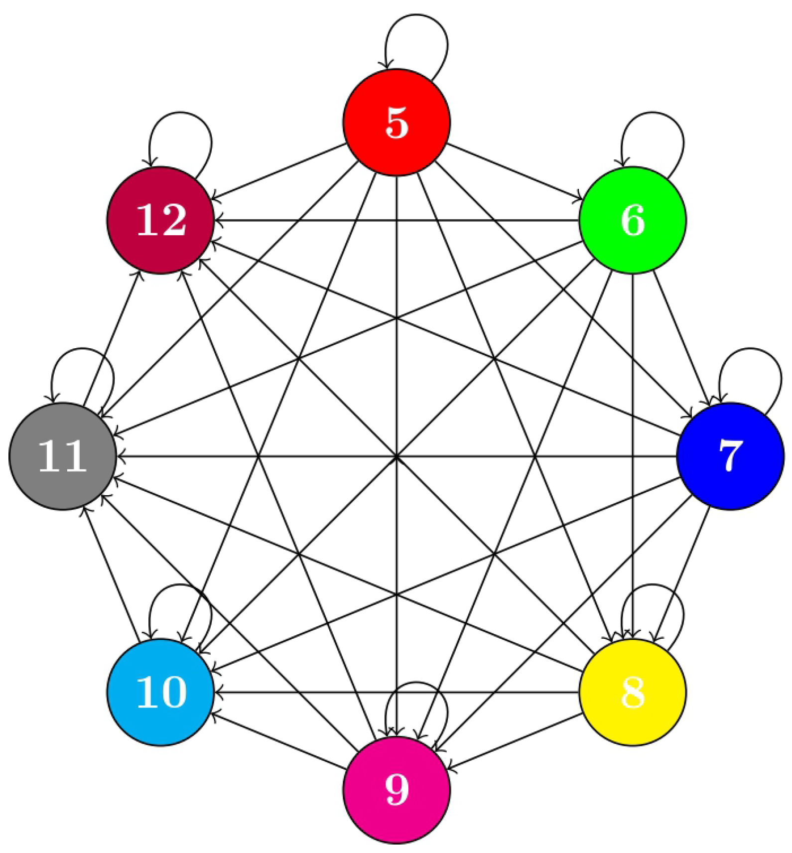
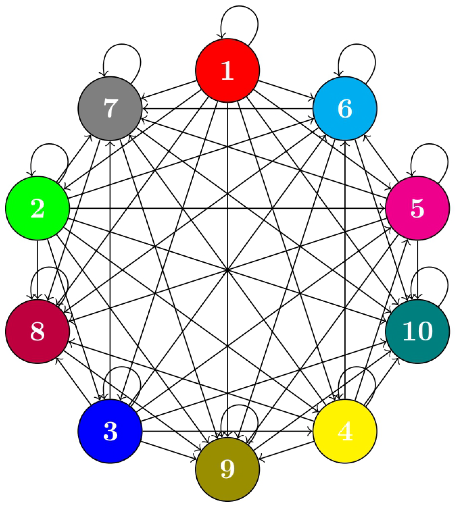
Example 1.

To reinforce the argument that a graphically extended suprametric space is not necessarily an extended suprametric space, consider the set $\coprod =\{1,2,3,4,5,6,7,8,9,10\}$ and the function $\psi :\coprod \times \coprod \to [1,\infty )$ as

$$\psi (\sout{\partial },\vartheta )={\displaystyle \frac{2}{\sout{\partial }\vartheta +2}}+1.975.$$

Also take into account the mapping $E_s^{\mathcal{G}}:\coprod \times \coprod \to [0,\infty )$ as

$$E_s^{\mathcal{G}}(\sout{\partial },\vartheta )=\left\{\begin{array}{cc}{\left|\sout{\partial }-\vartheta \right|}^2,\hfill & if\sout{\partial }\ne \vartheta \hfill \\ 0,\hfill & if\sout{\partial }=\vartheta .\hfill \end{array}\right.$$

The vertex set, denoted as $\coprod =\mathbb{V}\left(\mathcal{G}\right)$, along with the edge set, is constructed as illustrated in Figure 1.

The axioms (i)–(iii) of Definition 1 are obvious. To provide the axiom $\left(iv\right)$, fix $\sout{\partial },\vartheta \in \coprod$. In this axiom, the intermediate node z is taken on a directed path from $\sout{\partial }$ to ϑ in $\mathcal{G}$. Since $\mathcal{G}$ is complete with loops, the endpoints belong to every such path, hence the trivial choices $z=\sout{\partial }$ or $z=\vartheta$ are allowed.

$\left(i\right)$

Taking $z=\sout{\partial }$ we have $E_s^{\mathcal{G}}(\sout{\partial },z)=E_s^{\mathcal{G}}(\sout{\partial },\sout{\partial })=0$ and $E_s^{\mathcal{G}}(z,\vartheta )=E_s^{\mathcal{G}}(\sout{\partial },\vartheta )$, so

$$E_s^{\mathcal{G}}(\sout{\partial },\vartheta )\le E_s^{\mathcal{G}}(\sout{\partial },z)+E_s^{\mathcal{G}}(z,\vartheta )+\psi (\sout{\partial },\vartheta )E_s^{\mathcal{G}}(\sout{\partial },z)E_s^{\mathcal{G}}(z,\vartheta )=0+E_s^{\mathcal{G}}(\sout{\partial },\vartheta )+\psi (\sout{\partial },\vartheta )·0,$$

i.e., the inequality of axiom $\left(iv\right)$ holds, indeed with equality. This proves $\left(iv\right)$ under the convention that the endpoint is an admissible intermediate node.

$\left(ii\right)$

If one also wishes to check $\left(iv\right)$ for every interior $z\ne \sout{\partial },\vartheta$, write $u=|\sout{\partial }-z|\ge 1$ and $v=|z-\vartheta |\ge 1$. Then

$$E_s^{\mathcal{G}}(\sout{\partial },\vartheta )={(u+v)}^2,E_s^{\mathcal{G}}(\sout{\partial },z)=u^2,E_s^{\mathcal{G}}(z,\vartheta )=v^2,$$

and axiom $\left(iv\right)$ becomes

$${(u+v)}^2\le u^2+v^2+\psi (\sout{\partial },\vartheta )u^2{v}^2⟺2uv\le \psi (\sout{\partial },\vartheta )u^2{v}^2.$$

Since $u,v\ge 1$, a sufficient uniform condition is $\psi (\sout{\partial },\vartheta )\ge 2$. For our choice

$$\psi (\sout{\partial },\vartheta )={\displaystyle \frac{2}{xy+2}}+1.975,$$

we have

$$\psi (\sout{\partial },\vartheta )\in \left[1.975+\frac{2}{102},1.975+\frac{2}{3}\right]=[1.9946\dots ,2.6416\dots ].$$

Hence, for all pairs with $\sout{\partial }\vartheta \le 78$, we have $\psi (\sout{\partial },\vartheta )\ge 2$, and $\left(iv\right)$ holds for every interior z. For pairs with $\sout{\partial }\vartheta \ge 79$, $\psi (\sout{\partial },\vartheta )$ may drop below 2; in that case $\left(iv\right)$ still holds by part (a), by choosing the endpoint $z=\sout{\partial }$ or $z=\vartheta$. If we prefer a uniform interior z guarantee for all pairs, it suffices to replace the constant $1.975$ by 2 in ψ, making $min\psi >2$ on $\coprod \times \coprod$.

Clearly, $(\coprod ,E_s^{\mathcal{G}})$ is a graphically extended suprametric space but not an extended suprametric space since

$$\begin{array}{ccc}\hfill E_s^{\mathcal{G}}(8,10)& \nleqq & E_s^{\mathcal{G}}(8,9)+E_s^{\mathcal{G}}(9,10)+\psi (8,10)E_s^{\mathcal{G}}(8,9)E_s^{\mathcal{G}}(9,10).\hfill \end{array}$$

The example above illustrates that the graphical structure we have introduced provides a more enriched and nuanced perspective compared to existing literature.

2. Fixed Point Results Related to Graphical Structures

Fixed point theory in its classical form has largely been developed within the framework of complete metric or normed spaces, assuming global interaction among all elements of the space. However, many contemporary problems especially those arising in economic networks, control systems, and discrete dynamical models feature structural constraints that are more accurately represented by directed graphs. Motivated by these considerations, this section focuses on fixed point results formulated in the setting of graphically extended suprametric spaces. These spaces generalize both suprametric and metric-topological frameworks by incorporating directional connectivity through a graph, allowing for asymmetric and localized interactions. We introduce three distinct types of contractive mappings, graphical supra-Kannan, supra-Reich, and supra-Ciric contractions, each preserving the graphical structure and satisfying modified contractive conditions suited to the suprametric setting. For each mapping type, we establish the existence and uniqueness results for fixed points under appropriate assumptions, supported by rigorous proofs. These results extend classical theorems and offer a unified approach to analyzing fixed point behavior in structured, graph-based structures.

Let $\mathcal{G}=\left(\mathbb{V}\right(\mathcal{G}),\Xi (\mathcal{G}\left)\right)$ be a weighted graph that includes all of its loops. Suppose that a sequence ${\left\{v_n\right\}}_{n\in \mathbb{N}}$ in ∐ is generated by the rule $v_n={\Im }^n{v}_0$ for all $n\in \mathbb{N}$, starting from an initial point $v_0\in \coprod$. Then, the sequence ${\left\{v_n\right\}}_{n\in \mathbb{N}}$ is referred to as a ℑ–Picard sequence $(\Im -PS)$ corresponding to the self map $\Im :\coprod \to \coprod$.

Suppose that the $\mathcal{G}$–term-wise associated sequence $\Im -PS{\left\{v_n\right\}}_{n\in \mathbb{N}}$ is convergent in $\mathbb{C}$. Then, there exists a limit point $\nu \in \coprod$ of the sequence ${\left\{v_n\right\}}_{n\in \mathbb{N}}$, and there exists $n_0\in \mathbb{N}$ such that for every $n>n_0$, either $(v_n,v)\in \Xi \left(\mathcal{G}\right)$ or $(v,v_n)\in \Xi \left(\mathcal{G}\right)$. In such a case, the structure $\mathcal{G}=\left(\mathbb{V}\right(\mathcal{G}),\Xi (\mathcal{G}\left)\right)$ is said to satisfy the property $\left(\mathcal{A}\right)$.

Remark 3.

Assume that $\psi :\mathbb{V}\left(\mathcal{G}\right)\times \mathbb{V}\left(\mathcal{G}\right)\to [1,\infty )$ is bounded on the set visited by the sequence by a constant ${\psi }_{max}$, where ${\psi }_{max}$ is the maximum value of the function ψ, and that the sequence lies in a single $\mathcal{G}-$component which means that the sequence is $\mathcal{G}-$termwise connected, or the graph satisfies property $\left(\mathcal{A}\right)$. For ${\left(\sout{\partial }\mathcal{P}\vartheta \right)}_{\mathcal{G}}$ and any z on a directed path from $\sout{\partial }$ to ϑ, we have

$$E_s^{\mathcal{G}}(\sout{\partial },\vartheta )\le E_s^{\mathcal{G}}(\sout{\partial },z)+E_s^{\mathcal{G}}(z,\vartheta )+\psi (\sout{\partial },\vartheta )E_s^{\mathcal{G}}(\sout{\partial },z)E_s^{\mathcal{G}}(z,\vartheta ).$$

Let ${\left\{{\sout{\partial }}_{\nu }\right\}}_{n\in \mathbb{N}}$ be Cauchy in $(\mathbb{V}\left(\mathcal{G}\right),E_s^{\mathcal{G}})$. Given $\epsilon >0$ choose N so that $E_s^{\mathcal{G}}({\sout{\partial }}_{\nu },{\sout{\partial }}_{\mu })<\epsilon$ for all $\nu ,\mu >N$. For $k>\mu >\nu >N$, property $\left(\mathcal{A}\right)$ or $\mathcal{G}-$$\mathcal{AWC}$ yields a directed path from ${\sout{\partial }}_{\nu }$ to ${\sout{\partial }}_k$ containing some point z; applying the inequality at that z gives

$$E_s^{\mathcal{G}}({\sout{\partial }}_{\nu },{\sout{\partial }}_k)\le E_s^{\mathcal{G}}({\sout{\partial }}_{\nu },{\sout{\partial }}_{\mu })+E_s^{\mathcal{G}}({\sout{\partial }}_{\mu },{\sout{\partial }}_k)+\psi ({\sout{\partial }}_{\nu },{\sout{\partial }}_k)E_s^{\mathcal{G}}({\sout{\partial }}_{\nu },{\sout{\partial }}_{\mu })E_s^{\mathcal{G}}({\sout{\partial }}_{\mu },{\sout{\partial }}_k)\le 2\epsilon +{\psi }_{max}{\epsilon }^2.$$

As $\epsilon \to 0$, the right–hand side tends to 0; hence ${\left\{{\sout{\partial }}_{\nu }\right\}}_{n\in \mathbb{N}}$ remains Cauchy.

If ${\sout{\partial }}_{\nu }\to \sout{\partial }$ in $E_s^{\mathcal{G}}$, then for large $\nu ,\mu$,

$$E_s^{\mathcal{G}}({\sout{\partial }}_{\nu },{\sout{\partial }}_{\mu })\le E_s^{\mathcal{G}}({\sout{\partial }}_{\nu },\sout{\partial })+E_s^{\mathcal{G}}(\sout{\partial },{\sout{\partial }}_{\mu })+\psi ({\sout{\partial }}_{\nu },{\sout{\partial }}_{\mu })E_s^{\mathcal{G}}({\sout{\partial }}_{\nu },\sout{\partial })E_s^{\mathcal{G}}(\sout{\partial },{\sout{\partial }}_{\mu })\le 2\epsilon +{\psi }_{max}{\epsilon }^2,$$

which shows that the sequence is Cauchy.

It is necessary to have the boundedness of ψ. If ψ is unbounded, the structure may fail. For instance, on $\mathbb{V}\left(\mathcal{G}\right)=\mathbb{R}$ with $E_s^{\mathcal{G}}(\sout{\partial },\vartheta )=|\sout{\partial }-\vartheta |$ and $\psi (\sout{\partial },\vartheta )=1/|\sout{\partial }-\vartheta |$, ψ diverges as $\vartheta \to \sout{\partial }$ and the inequality cannot control $E_s^{\mathcal{G}}(\sout{\partial },\vartheta )$; boundedness or boundedness along the sequence is therefore essential for preserving convergence and completeness.

Definition 3.

Consider the mapping $\Im :\coprod \to \coprod$ on a graphically extended suprametric space $(\coprod ,E_s^{\mathcal{G}})$, which is identified as a graphical supra-Kannan contraction characterized by the following aspects

$\left(i\right)$

for all $\sout{\partial },\vartheta \in \coprod$ if

$$(\sout{\partial },\vartheta )\in \Xi \left(\mathcal{G}\right)\Rightarrow (\Im \sout{\partial },\Im \vartheta )\in \Xi \left(\mathcal{G}\right),$$

which ensures that ℑ preserves $\Xi \left(\mathcal{G}\right),$

$\left(ii\right)$

for all $\sout{\partial },\vartheta \in \coprod$ with $(\sout{\partial },\vartheta )\in \Xi \left(\mathcal{G}\right),$ there exists $\beta \in \left(0,{\displaystyle \frac{1}{2}}\right)$ ensures that

$$E_s^{\mathcal{G}}\left(\Im \sout{\partial },\Im \vartheta \right)\le \beta \left[E_s^{\mathcal{G}}\left(\sout{\partial },\Im \sout{\partial }\right)+E_s^{\mathcal{G}}\left(\vartheta ,\Im \vartheta \right)\right].$$

Remark 4.

If $\mathcal{G}$ is a complete undirected graph and $\psi \equiv 0$, taking $E_s^{\mathcal{G}}=d$, which d is a metric, reduces our contractive condition to the classical Kannan inequality $d(\Im \sout{\partial },\Im \vartheta )\le \kappa \left[d\right(\sout{\partial },\Im \sout{\partial })+d(\vartheta ,\Im \vartheta \left)\right]$ with $0<\kappa <\frac{1}{2}$. Moreover, the proof of uniqueness of the limit uses the symmetric control by $E_s^{\mathcal{G}}(v,v_n)$ and $E_s^{\mathcal{G}}(w,v_n)$; hence both defect terms are indispensable in the graph or asymmetric settings. Removing either term may compromise the result.

Theorem 1.

Consider a mapping $\Im :\coprod \to \coprod$, which is classified as a graphical supra-Kannan contraction within a complete graphically extended suprametric space $(\coprod ,E_s^{\mathcal{G}})$. Assume that the associated graph $\mathcal{G}$ possesses the property $\left(\mathcal{A}\right)$. Under these circumstances, there exists an element ${\sout{\partial }}_0\in \coprod$ such that $\Im {\sout{\partial }}_0\in {\left[{\sout{\partial }}_0\right]}_{\mathcal{G}}^l$, for some $l\in \mathbb{N}$. Furthermore, it can be established that there exists an element ${\sout{\partial }}^{\prime }\in \coprod$, for which the sequence ${\left\{{\sout{\partial }}_{\nu }\right\}}_{\nu \in \mathbb{N}}$ is an $\Im -PS$ sequence, satisfying the condition of being $\mathcal{G}-\mathcal{AWC}$, and converges to the limit ${\sout{\partial }}^{\prime }$.

Proof. 

Let ${\sout{\partial }}_0\in \coprod$ be selected such that $\Im {\sout{\partial }}_0\in {\left[{\sout{\partial }}_0\right]}_{\mathcal{G}}^l$ for a given $l\in \mathbb{N}$. Denote the initial point of our analysis as ${\sout{\partial }}_0$, derived from the Picard sequence ${\left\{{\sout{\partial }}_{\nu }\right\}}_{\nu \in \mathbb{N}}$ associated with ℑ. We assert the existence of a sequence of path elements ${\left\{{\eta }_{\rho }\right\}}_{\rho =0}^l$, such that ${\sout{\partial }}_0={\eta }_0$ and $\Im {\sout{\partial }}_0={\eta }_1$. Furthermore, we find that for each $\rho =1,2,\dots ,l$, the pair $({\eta }_{\rho -1},{\eta }_{\rho })$ belongs to the set $\Xi \left(\mathcal{G}\right)$, thus establishing valid connectivity within the framework of the given graph structure. Since ℑ preserves edge of $\mathcal{G}$, we see that $(\Im {\eta }_{\rho -1},\Im {\eta }_{\rho })\in \Xi \left(\mathcal{G}\right)$ for $\rho =1,2,\dots ,l.$ This indicates that ${\{\Im {\eta }_{\rho }\}}_{\rho =0}^l$ is a path from $\Im {\eta }_0=\Im {\sout{\partial }}_0={\sout{\partial }}_1$ to $\Im {\eta }_1={\Im }^2{\sout{\partial }}_0$$={\sout{\partial }}_2$ characterized by a length l with the result that ${\sout{\partial }}_2\in {\left[{\sout{\partial }}_1\right]}_{\mathcal{G}}^l.$ In this manner, we conclude that the sequence ${\left\{{\Im }^{\nu }{\eta }_{\rho }\right\}}_{\rho =0}^l$ constitutes a path connecting the points ${\Im }^{\nu }{\sout{\partial }}_0={\Im }^{\nu }{\eta }_0={\sout{\partial }}_{\nu }$ and ${\Im }^{\nu }{\sout{\partial }}_1={\Im }^{\nu }\Im {\eta }_0={\sout{\partial }}_{\nu +1}$ with a length of l. Consequently, we establish ${\sout{\partial }}_{\nu +1}\in {\left[{\sout{\partial }}_{\nu }\right]}_{\mathcal{G}}^l$ for every $\nu \in \mathbb{N}$. This implies that the sequence ${\left\{{\sout{\partial }}_{\nu }\right\}}_{\nu \in \mathbb{N}}$ fulfills the property of $\mathcal{G}-\mathcal{AWC}$, signifies that for $\rho =1,2,\dots ,l$ and $\nu \in \mathbb{N}$

$$({\Im }^{\nu }{\sout{\partial }}_{\rho -1},{\Im }^{\nu }{\sout{\partial }}_{\rho })\in \Xi \left(\mathcal{G}\right).$$

Utilizing the contractive condition of graphical supra-Kannan contraction, we arrive at

$$\begin{array}{c}{E}_s^{\mathcal{G}}\left({\Im }^{\nu }{\sout{\partial }}_{\rho -1},{\Im }^{\nu }{\sout{\partial }}_{\rho }\right)=E_s^{\mathcal{G}}\left(\Im \left({\Im }^{\nu -1}{\sout{\partial }}_{\rho -1}\right),\Im \left({\Im }^{\nu -1}{\sout{\partial }}_{\rho }\right)\right)\hfill \\ \\ \le \beta \left[E_s^{\mathcal{G}}\left({\Im }^{\nu -1}{\sout{\partial }}_{\rho -1},\Im \left({\Im }^{\nu -1}{\sout{\partial }}_{\rho -1}\right)\right)+E_s^{\mathcal{G}}\left({\Im }^{\nu -1}{\sout{\partial }}_{\rho },\Im \left({\Im }^{\nu -1}{\sout{\partial }}_{\rho }\right)\right)\right]\hfill \\ \\ \le \beta \left[E_s^{\mathcal{G}}\left({\Im }^{\nu -1}{\sout{\partial }}_{\rho -1},{\Im }^{\nu -1}{\sout{\partial }}_{\rho }\right)+E_s^{\mathcal{G}}\left({\Im }^{\nu }{\sout{\partial }}_{\rho -1},{\Im }^{\nu }{\sout{\partial }}_{\rho }\right)\right]\hfill \end{array}$$

such that

$$E_s^{\mathcal{G}}\left({\Im }^{\nu }{\sout{\partial }}_{\rho -1},{\Im }^{\nu }{\sout{\partial }}_{\rho }\right)\le {\displaystyle \frac{\beta }{1-\beta }}{E}_s^{\mathcal{G}}\left({\Im }^{\nu -1}{\sout{\partial }}_{\rho -1},{\Im }^{\nu -1}{\sout{\partial }}_{\rho }\right).$$

Set ${\displaystyle \frac{\beta }{1-\beta }}=\alpha ,$ where $\alpha \in \left[0,1\right)$ then above inequality turns into

$$E_s^{\mathcal{G}}\left({\Im }^{\nu }{\sout{\partial }}_{\rho -1},{\Im }^{\nu }{\sout{\partial }}_{\rho }\right)\le \alpha E_s^{\mathcal{G}}\left({\Im }^{\nu -1}{\sout{\partial }}_{\rho -1},{\Im }^{\nu -1}{\sout{\partial }}_{\rho }\right).$$

Persisting with the same method until we get

$$E_s^{\mathcal{G}}\left({\Im }^{\nu }{\sout{\partial }}_{\rho -1},{\Im }^{\nu }{\sout{\partial }}_{\rho }\right)\le {\alpha }^{\nu }{E}_s^{\mathcal{G}}\left({\sout{\partial }}_{\rho -1},{\sout{\partial }}_{\rho }\right).$$

Using the triangle inequality of the graphical extended suprametric yields

$$\begin{array}{c}{E}_s^{\mathcal{G}}\left({\sout{\partial }}_{\nu },{\sout{\partial }}_{\nu +1}\right)=E_s^{\mathcal{G}}\left({\Im }^{\nu }{\sout{\partial }}_0,{\Im }^{\nu +1}{\sout{\partial }}_0\right)\hfill \\ \\ =E_s^{\mathcal{G}}\left({\Im }^{\nu }{\eta }_0,{\Im }^{\nu }{\eta }_l\right)\hfill \\ \\ \le E_s^{\mathcal{G}}\left({\Im }^{\nu }{\eta }_0,{\Im }^{\nu }{\eta }_1\right)+E_s^{\mathcal{G}}\left({\Im }^{\nu }{\eta }_1,{\Im }^{\nu }{\eta }_l\right)+\psi \left({\Im }^{\nu }{\eta }_0,{\Im }^{\nu }{\eta }_l\right)E_s^{\mathcal{G}}\left({\Im }^{\nu }{\eta }_0,{\Im }^{\nu }{\eta }_1\right)E_s^{\mathcal{G}}\left({\Im }^{\nu }{\eta }_1,{\Im }^{\nu }{\eta }_l\right)\hfill \\ \\ \le E_s^{\mathcal{G}}\left({\Im }^{\nu }{\eta }_0,{\Im }^{\nu }{\eta }_1\right)+E_s^{\mathcal{G}}\left({\Im }^{\nu }{\eta }_1,{\Im }^{\nu }{\eta }_2\right)+E_s^{\mathcal{G}}\left({\Im }^{\nu }{\eta }_2,{\Im }^{\nu }{\eta }_l\right)\hfill \\ \\ +\psi \left({\Im }^{\nu }{\eta }_1,{\Im }^{\nu }{\eta }_l\right)E_s^{\mathcal{G}}\left({\Im }^{\nu }{\eta }_1,{\Im }^{\nu }{\eta }_2\right)E_s^{\mathcal{G}}\left({\Im }^{\nu }{\eta }_2,{\Im }^{\nu }{\eta }_l\right)\hfill \\ \\ +\psi \left({\Im }^{\nu }{\eta }_0,{\Im }^{\nu }{\eta }_l\right)E_s^{\mathcal{G}}\left({\Im }^{\nu }{\eta }_0,{\Im }^{\nu }{\eta }_1\right)E_s^{\mathcal{G}}\left({\Im }^{\nu }{\eta }_1,{\Im }^{\nu }{\eta }_l\right).\hfill \end{array}$$

By repeating a similar process, we have

$$\begin{array}{c}{E}_s^{\mathcal{G}}\left({\sout{\partial }}_{\nu },{\sout{\partial }}_{\nu +1}\right)\le E_s^{\mathcal{G}}\left({\Im }^{\nu }{\eta }_0,{\Im }^{\nu }{\eta }_1\right)+E_s^{\mathcal{G}}\left({\Im }^{\nu }{\eta }_1,{\Im }^{\nu }{\eta }_2\right)+E_s^{\mathcal{G}}\left({\Im }^{\nu }{\eta }_2,{\Im }^{\nu }{\eta }_3\right)+...+E_s^{\mathcal{G}}\left({\Im }^{\nu }{\eta }_{l-1},{\Im }^{\nu }{\eta }_l\right)\hfill \\ +\psi \left({\Im }^{\nu }{\eta }_0,{\Im }^{\nu }{\eta }_l\right)E_s^{\mathcal{G}}\left({\Im }^{\nu }{\eta }_0,{\Im }^{\nu }{\eta }_1\right)E_s^{\mathcal{G}}\left({\Im }^{\nu }{\eta }_1,{\Im }^{\nu }{\eta }_l\right)\hfill \\ +\psi \left({\Im }^{\nu }{\eta }_1,{\Im }^{\nu }{\eta }_l\right)E_s^{\mathcal{G}}\left({\Im }^{\nu }{\eta }_1,{\Im }^{\nu }{\eta }_2\right)E_s^{\mathcal{G}}\left({\Im }^{\nu }{\eta }_2,{\Im }^{\nu }{\eta }_l\right)\hfill \\ +...+\psi \left({\Im }^{\nu }{\eta }_{l-2},{\Im }^{\nu }{\eta }_l\right)E_s^{\mathcal{G}}\left({\Im }^{\nu }{\eta }_{l-2},{\Im }^{\nu }{\eta }_{l-1}\right)E_s^{\mathcal{G}}\left({\Im }^{\nu }{\eta }_{l-1},{\Im }^{\nu }{\eta }_l\right)\hfill \\ \\ \le {\displaystyle \sum _{i=1}^l}{E}_s^{\mathcal{G}}\left({\Im }^{\nu }{\eta }_{i-1},{\Im }^{\nu }{\eta }_i\right)+{\displaystyle \sum _{i=1}^{l-1}}\psi \left({\Im }^{\nu }{\eta }_{i-1},{\Im }^{\nu }{\eta }_l\right)E_s^{\mathcal{G}}\left({\Im }^{\nu }{\eta }_{i-1},{\Im }^{\nu }{\eta }_i\right)E_s^{\mathcal{G}}\left({\Im }^{\nu }{\eta }_i,{\Im }^{\nu }{\eta }_l\right)\hfill \\ \\ \le {\displaystyle \sum _{i=1}^l}{\alpha }^{\nu }{E}_s^{\mathcal{G}}\left({\eta }_{i-1},{\eta }_i\right)+{\displaystyle \sum _{i=1}^{l-1}}\psi \left({\Im }^{\nu }{\eta }_{i-1},{\Im }^{\nu }{\eta }_l\right){\alpha }^{\nu }{E}_s^{\mathcal{G}}\left({\eta }_{i-1},{\eta }_i\right)E_s^{\mathcal{G}}\left({\Im }^{\nu }{\eta }_i,{\Im }^{\nu }{\eta }_l\right)\hfill \\ \\ ={\alpha }^{\nu }\left[{\displaystyle \sum _{i=1}^l}{E}_s^{\mathcal{G}}\left({\eta }_{i-1},{\eta }_i\right)+{\displaystyle \sum _{i=1}^{l-1}}\psi \left({\Im }^{\nu }{\eta }_{i-1},{\Im }^{\nu }{\eta }_l\right)E_s^{\mathcal{G}}\left({\eta }_{i-1},{\eta }_i\right)E_s^{\mathcal{G}}\left({\Im }^{\nu }{\eta }_i,{\Im }^{\nu }{\eta }_l\right)\right].\hfill \end{array}$$

Considering the construction of $\mathcal{G}-\mathcal{AWC}$ sequence, we obtain

$$\begin{array}{c}{E}_s^{\mathcal{G}}\left({\sout{\partial }}_{\nu },{\sout{\partial }}_{\mu }\right)\le E_s^{\mathcal{G}}\left({\sout{\partial }}_{\nu },{\sout{\partial }}_{\nu +1}\right)+E_s^{\mathcal{G}}\left({\sout{\partial }}_{\nu +1},{\sout{\partial }}_{\mu }\right)+\psi \left({\sout{\partial }}_{\nu },{\sout{\partial }}_{\mu }\right)E_s^{\mathcal{G}}\left({\sout{\partial }}_{\nu },{\sout{\partial }}_{\nu +1}\right)E_s^{\mathcal{G}}\left({\sout{\partial }}_{\nu +1},{\sout{\partial }}_{\mu }\right)\hfill \\ \\ \le {\alpha }^{\nu }\left[{\displaystyle \sum _{i=1}^l}{E}_s^{\mathcal{G}}\left({\eta }_{i-1},{\eta }_i\right)+{\displaystyle \sum _{i=1}^{l-1}}\psi \left({\Im }^{\nu }{\eta }_{i-1},{\Im }^{\nu }{\eta }_l\right)E_s^{\mathcal{G}}\left({\eta }_{i-1},{\eta }_i\right)E_s^{\mathcal{G}}\left({\Im }^{\nu }{\eta }_i,{\Im }^{\nu }{\eta }_l\right)\right]\hfill \\ +\left[1+\psi \left({\sout{\partial }}_{\nu },{\sout{\partial }}_{\mu }\right){\alpha }^{\nu }\left[{\displaystyle \sum _{i=1}^l}{E}_s^{\mathcal{G}}\left({\eta }_{i-1},{\eta }_i\right)+{\displaystyle \sum _{i=1}^{l-1}}\psi \left({\Im }^{\nu }{\eta }_{i-1},{\Im }^{\nu }{\eta }_l\right)E_s^{\mathcal{G}}\left({\eta }_{i-1},{\eta }_i\right)E_s^{\mathcal{G}}\left({\Im }^{\nu }{\eta }_i,{\Im }^{\nu }{\eta }_l\right)\right]\right]\hfill \\ \times E_s^{\mathcal{G}}\left({\sout{\partial }}_{\nu +1},{\sout{\partial }}_{\mu }\right)\hfill \end{array}$$

for all $\nu ,\mu \in \mathbb{N},$ and $\nu <\mu$, where

$$\begin{array}{c}{E}_s^{\mathcal{G}}\left({\sout{\partial }}_{\nu +1},{\sout{\partial }}_{\mu }\right)\le E_s^{\mathcal{G}}\left({\sout{\partial }}_{\nu +1},{\sout{\partial }}_{\nu +2}\right)+E_s^{\mathcal{G}}\left({\sout{\partial }}_{\nu +2},{\sout{\partial }}_{\mu }\right)+\psi \left({\sout{\partial }}_{\nu +1},{\sout{\partial }}_{\mu }\right)E_s^{\mathcal{G}}\left({\sout{\partial }}_{\nu +1},{\sout{\partial }}_{\nu +2}\right)E_s^{\mathcal{G}}\left({\sout{\partial }}_{\nu +2},{\sout{\partial }}_{\mu }\right)\hfill \\ \\ \le {\alpha }^{\nu +1}\left[{\displaystyle \sum _{i=1}^l}{E}_s^{\mathcal{G}}\left({\eta }_{i-1},{\eta }_i\right)+{\displaystyle \sum _{i=1}^{l-1}}\psi \left({\Im }^{\nu }{\eta }_{i-1},{\Im }^{\nu }{\eta }_l\right)E_s^{\mathcal{G}}\left({\eta }_{i-1},{\eta }_i\right)E_s^{\mathcal{G}}\left({\Im }^{\nu }{\eta }_i,{\Im }^{\nu }{\eta }_l\right)\right]\hfill \\ +\left[1+\psi \left({\sout{\partial }}_{\nu +1},{\sout{\partial }}_{\mu }\right){\alpha }^{\nu +1}\left[{\displaystyle \sum _{i=1}^l}{E}_s^{\mathcal{G}}\left({\eta }_{i-1},{\eta }_i\right)+{\displaystyle \sum _{i=1}^{l-1}}\psi \left({\Im }^{\nu }{\eta }_{i-1},{\Im }^{\nu }{\eta }_l\right)E_s^{\mathcal{G}}\left({\eta }_{i-1},{\eta }_i\right)E_s^{\mathcal{G}}\left({\Im }^{\nu }{\eta }_i,{\Im }^{\nu }{\eta }_l\right)\right]\right]\hfill \\ \times E_s^{\mathcal{G}}\left({\sout{\partial }}_{\nu +2},{\sout{\partial }}_{\mu }\right).\hfill \end{array}$$

Continuing the same process, the subsequent expression is derived

$$\begin{array}{c}{E}_s^{\mathcal{G}}\left({\sout{\partial }}_{\nu },{\sout{\partial }}_{\mu }\right)\le {\alpha }^{\nu }\left[{\displaystyle \sum _{i=1}^l}{E}_s^{\mathcal{G}}\left({\eta }_{i-1},{\eta }_i\right)+{\displaystyle \sum _{i=1}^{l-1}}\psi \left({\Im }^{\nu }{\eta }_{i-1},{\Im }^{\nu }{\eta }_l\right)E_s^{\mathcal{G}}\left({\eta }_{i-1},{\eta }_i\right)E_s^{\mathcal{G}}\left({\Im }^{\nu }{\eta }_i,{\Im }^{\nu }{\eta }_l\right)\right]\hfill \\ +{\alpha }^{\nu +1}\left[{\displaystyle \sum _{i=1}^l}{E}_s^{\mathcal{G}}\left({\eta }_{i-1},{\eta }_i\right)+{\displaystyle \sum _{i=1}^{l-1}}\psi \left({\Im }^{\nu }{\eta }_{i-1},{\Im }^{\nu }{\eta }_l\right)E_s^{\mathcal{G}}\left({\eta }_{i-1},{\eta }_i\right)E_s^{\mathcal{G}}\left({\Im }^{\nu }{\eta }_i,{\Im }^{\nu }{\eta }_l\right)\right]\hfill \\ \times \left[1+\psi \left({\sout{\partial }}_{\nu },{\sout{\partial }}_{\mu }\right){\alpha }^{\nu }\left[{\displaystyle \sum _{i=1}^l}{E}_s^{\mathcal{G}}\left({\eta }_{i-1},{\eta }_i\right)+{\displaystyle \sum _{i=1}^{l-1}}\psi \left({\Im }^{\nu }{\eta }_{i-1},{\Im }^{\nu }{\eta }_l\right)E_s^{\mathcal{G}}\left({\eta }_{i-1},{\eta }_i\right)E_s^{\mathcal{G}}\left({\Im }^{\nu }{\eta }_i,{\Im }^{\nu }{\eta }_l\right)\right]\right]\hfill \\ +{\alpha }^{\nu +2}\left[{\displaystyle \sum _{i=1}^l}{E}_s^{\mathcal{G}}\left({\eta }_{i-1},{\eta }_i\right)+{\displaystyle \sum _{i=1}^{l-1}}\psi \left({\Im }^{\nu }{\eta }_{i-1},{\Im }^{\nu }{\eta }_l\right)E_s^{\mathcal{G}}\left({\eta }_{i-1},{\eta }_i\right)E_s^{\mathcal{G}}\left({\Im }^{\nu }{\eta }_i,{\Im }^{\nu }{\eta }_l\right)\right]\hfill \\ \times \left[1+\psi \left({\sout{\partial }}_{\nu },{\sout{\partial }}_{\mu }\right){\alpha }^{\nu }\left[{\displaystyle \sum _{i=1}^l}{E}_s^{\mathcal{G}}\left({\eta }_{i-1},{\eta }_i\right)+{\displaystyle \sum _{i=1}^{l-1}}\psi \left({\Im }^{\nu }{\eta }_{i-1},{\Im }^{\nu }{\eta }_l\right)E_s^{\mathcal{G}}\left({\eta }_{i-1},{\eta }_i\right)E_s^{\mathcal{G}}\left({\Im }^{\nu }{\eta }_i,{\Im }^{\nu }{\eta }_l\right)\right]\right]\hfill \\ \times \left[1+\psi \left({\sout{\partial }}_{\nu +1},{\sout{\partial }}_{\mu }\right){\alpha }^{\nu +1}\left[{\displaystyle \sum _{i=1}^l}{E}_s^{\mathcal{G}}\left({\eta }_{i-1},{\eta }_i\right)+{\displaystyle \sum _{i=1}^{l-1}}\psi \left({\Im }^{\nu }{\eta }_{i-1},{\Im }^{\nu }{\eta }_l\right)E_s^{\mathcal{G}}\left({\eta }_{i-1},{\eta }_i\right)E_s^{\mathcal{G}}\left({\Im }^{\nu }{\eta }_i,{\Im }^{\nu }{\eta }_l\right)\right]\right]\hfill \\ +...+{\alpha }^{\mu -1}\left[{\displaystyle \sum _{i=1}^l}{E}_s^{\mathcal{G}}\left({\eta }_{i-1},{\eta }_i\right)+{\displaystyle \sum _{i=1}^{l-1}}\psi \left({\Im }^{\nu }{\eta }_{i-1},{\Im }^{\nu }{\eta }_l\right)E_s^{\mathcal{G}}\left({\eta }_{i-1},{\eta }_i\right)E_s^{\mathcal{G}}\left({\Im }^{\nu }{\eta }_i,{\Im }^{\nu }{\eta }_l\right)\right]\hfill \\ \times \left[1+\psi \left({\sout{\partial }}_{\nu },{\sout{\partial }}_{\mu }\right){\alpha }^{\nu }\left[{\displaystyle \sum _{i=1}^l}{E}_s^{\mathcal{G}}\left({\eta }_{i-1},{\eta }_i\right)+{\displaystyle \sum _{i=1}^{l-1}}\psi \left({\Im }^{\nu }{\eta }_{i-1},{\Im }^{\nu }{\eta }_l\right)E_s^{\mathcal{G}}\left({\eta }_{i-1},{\eta }_i\right)E_s^{\mathcal{G}}\left({\Im }^{\nu }{\eta }_i,{\Im }^{\nu }{\eta }_l\right)\right]\right]\hfill \\ \times \left[1+\psi \left({\sout{\partial }}_{\nu +1},{\sout{\partial }}_{\mu }\right){\alpha }^{\nu +1}\left[{\displaystyle \sum _{i=1}^l}{E}_s^{\mathcal{G}}\left({\eta }_{i-1},{\eta }_i\right)+{\displaystyle \sum _{i=1}^{l-1}}\psi \left({\Im }^{\nu }{\eta }_{i-1},{\Im }^{\nu }{\eta }_l\right)E_s^{\mathcal{G}}\left({\eta }_{i-1},{\eta }_i\right)E_s^{\mathcal{G}}\left({\Im }^{\nu }{\eta }_i,{\Im }^{\nu }{\eta }_l\right)\right]\right]\hfill \\ \times ...\times \left[1+\psi \left({\sout{\partial }}_{m-2},{\sout{\partial }}_{\mu }\right){\alpha }^{\mu -2}\left[{\displaystyle \sum _{i=1}^l}{E}_s^{\mathcal{G}}\left({\eta }_{i-1},{\eta }_i\right)+{\displaystyle \sum _{i=1}^{l-1}}\psi \left({\Im }^{\nu }{\eta }_{i-1},{\Im }^{\nu }{\eta }_l\right)E_s^{\mathcal{G}}\left({\eta }_{i-1},{\eta }_i\right)E_s^{\mathcal{G}}\left({\Im }^{\nu }{\eta }_i,{\Im }^{\nu }{\eta }_l\right)\right]\right]\hfill \\ \le {\alpha }^{\nu }\left[{\displaystyle \sum _{i=1}^l}{E}_s^{\mathcal{G}}\left({\eta }_{i-1},{\eta }_i\right)+{\displaystyle \sum _{i=1}^{l-1}}\psi \left({\Im }^{\nu }{\eta }_{i-1},{\Im }^{\nu }{\eta }_l\right)E_s^{\mathcal{G}}\left({\eta }_{i-1},{\eta }_i\right)E_s^{\mathcal{G}}\left({\Im }^{\nu }{\eta }_i,{\Im }^{\nu }{\eta }_l\right)\right]\hfill \\ \times {\displaystyle \sum _{i=0}^{\mu -\nu -1}}{\alpha }^i{\displaystyle \prod _{\rho =0}^{i-1}}\left[1+\psi \left({\sout{\partial }}_{\nu +\rho },{\sout{\partial }}_{\mu }\right){\alpha }^{\nu +\rho }\left[{\displaystyle \sum _{i=1}^l}{E}_s^{\mathcal{G}}\left({\eta }_{i-1},{\eta }_i\right)+{\displaystyle \sum _{i=1}^{l-1}}\psi \left({\Im }^{\nu }{\eta }_{i-1},{\Im }^{\nu }{\eta }_l\right)E_s^{\mathcal{G}}\left({\eta }_{i-1},{\eta }_i\right)E_s^{\mathcal{G}}\left({\Im }^{\nu }{\eta }_i,{\Im }^{\nu }{\eta }_l\right)\right]\right].\hfill \end{array}$$

Given that $\alpha \in \left[0,1\right)$, it can be readily demonstrated that the series ${\sum }_{i=0}^{\infty }{\mathcal{S}}_i$ converges according to the ratio test, which results in the term ${\mathcal{S}}_i$ being defined as follows:

$${\mathcal{S}}_i={\alpha }^i{\displaystyle \prod _{\rho =0}^{i-1}}\left[1+\psi \left({\sout{\partial }}_{\nu +\rho },{\sout{\partial }}_{\mu }\right){\alpha }^{\nu +\rho }\left[{\displaystyle \sum _{i=1}^l}{E}_s^{\mathcal{G}}\left({\eta }_{i-1},{\eta }_i\right)+{\displaystyle \sum _{i=1}^{l-1}}\psi \left({\Im }^{\nu }{\eta }_{i-1},{\Im }^{\nu }{\eta }_l\right)E_s^{\mathcal{G}}\left({\eta }_{i-1},{\eta }_i\right)E_s^{\mathcal{G}}\left({\Im }^{\nu }{\eta }_i,{\Im }^{\nu }{\eta }_l\right)\right]\right].$$

In conclusion, we establish that the expression $E_s^{\mathcal{G}}\left({\sout{\partial }}_{\nu },{\sout{\partial }}_{\mu }\right)$ approaches zero as n and m tend to infinity. This observation implies that the sequence ${\left\{{\sout{\partial }}_{\nu }\right\}}_{\nu \in \mathbb{N}}$ constitutes a Cauchy sequence. Since $(\coprod ,E_s^{\mathcal{G}})$ is a complete graphically extended suprametric space and from property $\left(\mathcal{A}\right)$, then ${\left\{{\sout{\partial }}_{\nu }\right\}}_{\nu \in \mathbb{N}}$ converges in ∐ at a certain point ${\sout{\partial }}^{\prime }\in \coprod ,$ for ${\nu }_0\in \mathbb{N}$ such that $\left({\sout{\partial }}_{\nu },{\sout{\partial }}^{\prime }\right)\in \Xi \left(\mathcal{G}\right)$ or $\left({\sout{\partial }}^{\prime },{\sout{\partial }}_{\nu }\right)\in \Xi \left(\mathcal{G}\right)$ for all $\nu >{\nu }_0$

$$\underset{\nu \to \infty }{lim}{E}_s^{\mathcal{G}}\left({\sout{\partial }}_{\nu },{\sout{\partial }}^{\prime }\right)=0,$$

revealing that ${\left\{{\sout{\partial }}_{\nu }\right\}}_{\nu \in \mathbb{N}}$ converges to ${\sout{\partial }}^{\prime }.$ □

Lemma 1.

Fix a directed graph $\mathcal{G}=(\mathbb{V},\Xi )$ with loops $(v,v)\in \Xi$ for all $v\in \mathbb{V}$ and a topology induced by $E_s^{\mathcal{G}}$. Consider the following statements:

$\left(i\right)$

For every self-map $\Im :\mathbb{V}\to \mathbb{V}$, every Picard sequence $v_n={\Im }^n{v}_0$ that converges to $v\in \mathbb{V}$ is eventually adjacent to v in at least one direction, i.e., $\exists n_0$ such that $\forall n>n_0$ either $(v_n,v)\in \Xi$ or $(v,v_n)\in \Xi$.

$\left(ii\right)$

For every sequence $\left({\sout{\partial }}_n\right)\subset \mathbb{V}$ with ${\sout{\partial }}_n\to v$, there exists $n_0$ such that for all $n>n_0$ either $({\sout{\partial }}_n,v)\in \Xi$ or $(v,{\sout{\partial }}_n)\in \Xi$.

Then (i) holds for all self-maps ℑ if and only if (ii) holds.

Proof. 

(i)⇒(ii): Let $\left({\sout{\partial }}_n\right)$ be any sequence with ${\sout{\partial }}_n\to v$. Define $\Im :\mathbb{V}\to \mathbb{V}$ by $\Im \left({\sout{\partial }}_n\right)={\sout{\partial }}_{n+1}$ for all $n\ge 0$ and $\Im \left(v\right)=v$; extend ℑ arbitrarily on $\mathbb{V}\setminus (\left\{v\right\}\cup \{{\sout{\partial }}_n:n\ge 0\})$. Then the Picard orbit of ${\sout{\partial }}_0$ is exactly $\left({\sout{\partial }}_n\right)$ and it converges to v. By (i), $\left({\sout{\partial }}_n\right)$ is adjacent to v in one direction, hence (ii).

(ii)⇒(i): If $v_n={\Im }^n{v}_0\to v$, then $\left(v_n\right)$ is a convergent sequence, so (ii) yields the desired eventual adjacency. □

Remark 5.

If for every $v\in \mathbb{V}$ there exists ${\rho }_v>0$ such that

$$\vartheta \in {\mathbb{B}}_{E_s^{\mathcal{G}}}(v,{\rho }_v)\setminus \left\{v\right\}⟹(\vartheta ,v)\in \Xi or(v,\vartheta )\in \Xi ,$$

then (ii) holds and hence Property $\left(\mathcal{A}\right)$ holds. Indeed, any sequence ${\sout{\partial }}_n\to v$ is eventually inside ${\mathbb{B}}_{E_s^{\mathcal{G}}}(v,{\rho }_v)$, thus eventually adjacent to v.

Example 2.

Let $\mathbb{V}=[0,1]$, equip $\mathbb{V}$ with the standard $E_s^{\mathcal{G}}(\sout{\partial },\vartheta )=|\sout{\partial }-\vartheta |$, and take

$$\Xi =\left\{\right(\sout{\partial },\sout{\partial }):\sout{\partial }\in [0,1\left]\right\}$$

including loops only. Define $\Im \left(\sout{\partial }\right)=\sout{\partial }/2$ and $v_0=1$. Then $v_n=2^{-n}\to v=0$, however for all n we have $v_n\ne v$ and neither $(v_n,v)$ nor $(v,v_n)$ belongs to Ξ. Hence neither (ii) nor (i) holds in this graph.

Remark 6.

In the proof of our fixed point theorems, (i) is used only to apply the graphical inequality along the sequence of an orbit that converges to its limit v. Therefore, the following version is sufficient for the results: there exists $n_0$ (depending on the particular orbit) such that for all $n>n_0$ either $(v_n,v)\in \Xi$ or $(v,v_n)\in \Xi$. When (i) fails globally as in the example above, a Picard orbit may converge in the $E_s^{\mathcal{G}}$-topology but adjacency to v may never occur, and the limit transition in the graph-dependent inequality can break, possibly destroying uniqueness or existence in the intended component.

Lemma 2.

Let ${\left\{v_n\right\}}_{n\in \mathbb{N}}$ be the $\mathcal{G}$–$\mathcal{AWC}$ Picard sequence. If $v_n\to v$ and $v_n\to w$ in $(\mathbb{V},E_s^{\mathcal{G}})$, then $v=w$. Indeed, for any $\epsilon >0$ and large n,

$$E_s^{\mathcal{G}}(v,w)\le E_s^{\mathcal{G}}(v,v_n)+E_s^{\mathcal{G}}(v_n,w)+\psi (v,w)E_s^{\mathcal{G}}(v,v_n)E_s^{\mathcal{G}}(v_n,w)\le 2\epsilon +\psi (v,w){\epsilon }^2,$$

hence $E_s^{\mathcal{G}}(v,w)=0$ and so $v=w$.

This is consistent with the following definition, which already asserts the uniqueness of the limit for the Picard sequence.

Definition 4.

Let $(\coprod ,E_s^{\mathcal{G}})$ be a graphically extended suprametric space, and $\Im :\coprod \to \coprod$ be a self-mapping. The triplet $(\coprod ,E_s^{\mathcal{G}},\Im )$ is said to satisfy the property $\left({\mathcal{A}}^{*}\right)$ if the following condition holds:

• For any two limits ${\sout{\partial }}^{\prime }\in \coprod$ and ${\vartheta }^{\prime }\in \Im (\coprod )$ of a term-wise Picard sequence, it must be that ${\sout{\partial }}^{\prime }={\vartheta }^{\prime }.$

In other words, if a Picard-type iteration of ℑ admits two potential limit points, then these limits must coincide. This ensures the uniqueness of the limit and hence strengthens the convergence behavior of ℑ.

Theorem 2.

In accordance with the provisions delineated in Theorem 1, should all criteria be met concerning the triplet $(\coprod ,E_s^{\mathcal{G}},\Im )$ that demonstrates the property $\left({\mathcal{A}}^{*}\right)$, it can be conclusively inferred that the operator ℑ admits a fixed point.

Proof. 

Theorem 1 establishes that $\Im -$Picard sequence, initiated at the point ${\sout{\partial }}_0$, converges to both instances of ${\sout{\partial }}^{\prime }$ and $\Im {\sout{\partial }}^{\prime }$. Given that $\mathcal{G}$ is connected either ${({\sout{\partial }}^{\prime }\mathcal{P}\Im {\sout{\partial }}^{\prime })}_{\mathcal{G}}\in \Xi \left(\mathcal{G}\right)$ or ${(\Im {\sout{\partial }}^{\prime }\mathcal{P}{\sout{\partial }}^{\prime })}_{\mathcal{G}}\in \Xi \left(\mathcal{G}\right),$ then we arrive at

$$\begin{array}{c}{E}_s^{\mathcal{G}}\left({\sout{\partial }}^{\prime },\Im {\sout{\partial }}^{\prime }\right)\le E_s^{\mathcal{G}}\left({\sout{\partial }}^{\prime },{\sout{\partial }}_{\nu }\right)+E_s^{\mathcal{G}}\left({\sout{\partial }}_{\nu },\Im {\sout{\partial }}^{\prime }\right)+\psi \left({\sout{\partial }}^{\prime },\Im {\sout{\partial }}^{\prime }\right)E_s^{\mathcal{G}}\left({\sout{\partial }}^{\prime },{\sout{\partial }}_{\nu }\right)E_s^{\mathcal{G}}\left({\sout{\partial }}_{\nu },\Im {\sout{\partial }}^{\prime }\right)\hfill \\ \\ =E_s^{\mathcal{G}}\left({\sout{\partial }}^{\prime },{\sout{\partial }}_{\nu }\right)+E_s^{\mathcal{G}}\left(\Im {\sout{\partial }}_{\nu -1},\Im {\sout{\partial }}^{\prime }\right)+\psi \left({\sout{\partial }}^{\prime },\Im {\sout{\partial }}^{\prime }\right)E_s^{\mathcal{G}}\left({\sout{\partial }}^{\prime },{\sout{\partial }}_{\nu }\right)E_s^{\mathcal{G}}\left({\sout{\partial }}_{\nu },\Im {\sout{\partial }}^{\prime }\right).\hfill \end{array}$$

Utilizing the definition of a graphical supra Kannan contraction, we derive the following implications

$$\begin{array}{c}{E}_s^{\mathcal{G}}\left({\sout{\partial }}^{\prime },\Im {\sout{\partial }}^{\prime }\right)\le E_s^{\mathcal{G}}\left({\sout{\partial }}^{\prime },{\sout{\partial }}_{\nu }\right)+\beta \left[E_s^{\mathcal{G}}\left({\sout{\partial }}_{\nu -1},\Im {\sout{\partial }}_{\nu -1}\right)+E_s^{\mathcal{G}}\left({\sout{\partial }}^{\prime },\Im {\sout{\partial }}^{\prime }\right)\right]+\psi \left({\sout{\partial }}^{\prime },\Im {\sout{\partial }}^{\prime }\right)E_s^{\mathcal{G}}\left({\sout{\partial }}^{\prime },{\sout{\partial }}_{\nu }\right)E_s^{\mathcal{G}}\left({\sout{\partial }}_{\nu },\Im {\sout{\partial }}^{\prime }\right)\hfill \\ \\ =E_s^{\mathcal{G}}\left({\sout{\partial }}^{\prime },{\sout{\partial }}_{\nu }\right)+\beta E_s^{\mathcal{G}}\left({\sout{\partial }}_{\nu -1},\Im {\sout{\partial }}_{\nu -1}\right)+\beta E_s^{\mathcal{G}}\left({\sout{\partial }}^{\prime },\Im {\sout{\partial }}^{\prime }\right)+\psi \left({\sout{\partial }}^{\prime },\Im {\sout{\partial }}^{\prime }\right)E_s^{\mathcal{G}}\left({\sout{\partial }}^{\prime },{\sout{\partial }}_{\nu }\right)E_s^{\mathcal{G}}\left({\sout{\partial }}_{\nu },\Im {\sout{\partial }}^{\prime }\right).\hfill \end{array}$$

After straightforward calculations, we obtain

$$E_s^{\mathcal{G}}\left({\sout{\partial }}^{\prime },\Im {\sout{\partial }}^{\prime }\right)\le \left({\displaystyle \frac{E_s^{\mathcal{G}}\left({\sout{\partial }}^{\prime },{\sout{\partial }}_{\nu }\right)+\beta E_s^{\mathcal{G}}\left({\sout{\partial }}_{\nu -1},\Im {\sout{\partial }}_{\nu -1}\right)+\psi \left({\sout{\partial }}^{\prime },\Im {\sout{\partial }}^{\prime }\right)E_s^{\mathcal{G}}\left({\sout{\partial }}^{\prime },{\sout{\partial }}_{\nu }\right)E_s^{\mathcal{G}}\left({\sout{\partial }}_{\nu },\Im {\sout{\partial }}^{\prime }\right)}{1-\beta }}\right).$$

Taking limit $\nu \to \infty ,$ we have

$$E_s^{\mathcal{G}}\left({\sout{\partial }}^{\prime },\Im {\sout{\partial }}^{\prime }\right)=0.$$

It can be concluded that ${\sout{\partial }}^{\prime }$ serves as a fixed point of the mapping ℑ. □

Remark 7.

Under the property $\left({\mathcal{A}}^{*}\right)$ and using a bounded ψ, if ${sup}_{\sout{\partial }}{E}_s^{\mathcal{G}}(\Im \sout{\partial },\tilde{\Im }\sout{\partial })\le \epsilon$ and both maps satisfy the supra–Kannan condition with $\beta <\frac{1}{2}$, then their fixed points differ by at most $\epsilon /(1-\beta /(1-\beta \left)\right)$ in $E_s^{\mathcal{G}}$; hence the fixed point depends continuously on ℑ.

Example 3.

Consider the set $\coprod =\{11,12,13,14,15,16\}$ and the mapping $\psi :\coprod \times \coprod \to [1,\infty )$ such that

$$\psi (\sout{\partial },\vartheta )={\displaystyle \frac{1.95}{\sout{\partial }\vartheta +0.7}}+1.99.$$

Assume that the mapping $E_s^{\mathcal{G}}:\coprod \times \coprod \to [0,\infty )$ given as

$$E_s^{\mathcal{G}}(\sout{\partial },\vartheta )=\left\{\begin{array}{cc}{\left|\sout{\partial }-\vartheta \right|}^2,\hfill & if\sout{\partial }\ne \vartheta \hfill \\ 0,\hfill & if\sout{\partial }=\vartheta .\hfill \end{array}\right.$$

The vertex set, denoted by $\coprod =\mathbb{V}\left(\mathcal{G}\right)$, along with the edge set $\Xi \left(\mathcal{G}\right)$, is illustrated in Figure 2.

Clearly, $(\coprod ,E_s^{\mathcal{G}})$ is a graphically extended suprametric space but not an extended suprametric space since

$$\begin{array}{ccc}\hfill E_s^{\mathcal{G}}(14,16)& \nleqq & E_s^{\mathcal{G}}(14,15)+E_s^{\mathcal{G}}(15,16)+\psi (14,16)E_s^{\mathcal{G}}(14,15)E_s^{\mathcal{G}}(15,16).\hfill \end{array}$$

For the contractive condition, define a mapping $\Im :\coprod \to \coprod$ as

$$\Im \left(\sout{\partial }\right)=\left\{\begin{array}{cc}11,& for\sout{\partial }=13,\\ 12,& for\sout{\partial }\in \{12,15,16\}.\end{array}\right.$$

Case (i) For $\sout{\partial }=13$ and $\vartheta =12$, we have

$$\begin{array}{ccc}\hfill E_s^{\mathcal{G}}(\Im 13,\Im 12)& \le & \beta [E_s^{\mathcal{G}}(13,\Im 13)+E_s^{\mathcal{G}}(12,\Im 12)]\hfill \\ \hfill E_s^{\mathcal{G}}(11,12)& \le & \beta [E_s^{\mathcal{G}}(13,11)+E_s^{\mathcal{G}}(12,12)]\hfill \\ \hfill 1& \le & \beta \left(4\right)\Rightarrow \beta \ge \frac{1}{4}.\hfill \end{array}$$

Case (ii) If $\sout{\partial }=13$ and $\vartheta =15$, we get

$$\begin{array}{ccc}\hfill E_s^{\mathcal{G}}(\Im 13,\Im 15)& \le & \beta [E_s^{\mathcal{G}}(13,\Im 13)+E_s^{\mathcal{G}}(15,\Im 15)]\hfill \\ \hfill E_s^{\mathcal{G}}(11,12)& \le & \beta [E_s^{\mathcal{G}}(13,11)+E_s^{\mathcal{G}}(15,12)]\hfill \\ \hfill 1& \le & \beta \left(13\right)\Rightarrow \beta \ge \frac{1}{13}.\hfill \end{array}$$

Case (iii) When $\sout{\partial }=13$ and $\vartheta =16$, we obtain

$$\begin{array}{ccc}\hfill E_s^{\mathcal{G}}(\Im 13,\Im 16)& \le & \beta [E_s^{\mathcal{G}}(13,\Im 13)+E_s^{\mathcal{G}}(16,\Im 16)]\hfill \\ \hfill E_s^{\mathcal{G}}(11,12)& \le & \beta [E_s^{\mathcal{G}}(13,11)+E_s^{\mathcal{G}}(16,12)]\hfill \\ \hfill 1& \le & \beta \left(20\right)\Rightarrow \beta \ge \frac{1}{20}.\hfill \end{array}$$

All conditions have been satisfied for the parameter $\beta ={\displaystyle \frac{1}{4}}$, which is within the interval $(0,{\displaystyle \frac{1}{2}})$. Consequently, all the criteria outlined in Theorem 2 are fulfilled, confirming that “12” is the unique fixed point of the mapping ℑ.

Definition 5.

ℑ, a self-mapping defined on the graphically extended suprametric space $(\coprod ,E_s^{\mathcal{G}})$ is claimed as a graphical supra-Reich contraction, which is characterized by the following aspects

$\left(i\right)$

for all $\sout{\partial },\vartheta \in \coprod$ if

$$(\sout{\partial },\vartheta )\in \Xi \left(\mathcal{G}\right)\Rightarrow (\Im \sout{\partial },\Im \vartheta )\in \Xi \left(\mathcal{G}\right),$$

ensuring that ℑ preserves $\Xi \left(\mathcal{G}\right),$

$\left(ii\right)$

for all $\sout{\partial },\vartheta \in \coprod$ with $(\sout{\partial },\vartheta )\in \Xi \left(\mathcal{G}\right)$ there exist non-negative constants ${\beta }_1+{\beta }_2+{\beta }_3<1,$ ensures that

$$E_s^{\mathcal{G}}\left(\Im \sout{\partial },\Im \vartheta \right)\le {\beta }_1{E}_s^{\mathcal{G}}\left(\sout{\partial },\vartheta \right)+{\beta }_2{E}_s^{\mathcal{G}}\left(\sout{\partial },\Im \sout{\partial }\right)+{\beta }_3{E}_s^{\mathcal{G}}\left(\vartheta ,\Im \vartheta \right).$$

Theorem 3.

Let $\Im :\coprod \to \coprod$ denote a self-mapping characterized as a graphical supra-Reich contraction within a complete graphically extended suprametric space $(\coprod ,E_s^{\mathcal{G}})$. Assume that the graph $\mathcal{G}$ possesses the property denoted as $\left(\mathcal{A}\right)$. Under this assumption, there exists an element ${\sout{\partial }}_0\in \coprod$ such that $\Im \left({\sout{\partial }}_0\right)\in {\left[{\sout{\partial }}_0\right]}_{\mathcal{G}}^l$, for some integer $l\in \mathbb{N}$. Furthermore, there exists an element ${\sout{\partial }}^{\prime }\in \coprod$ such that the sequence $\Im -PS\left\{{\sout{\partial }}_{\nu }\right\}$ is $\mathcal{G}-\mathcal{AWC}$ and converges to ${\sout{\partial }}^{\prime }$.

Proof. 

The first part of the proof follows the same structural argument presented in Theorem 1, establishing the existence of a Picard sequence ${\left\{{\sout{\partial }}_{\nu }\right\}}_{\nu \in \mathbb{N}}$ such that ${\sout{\partial }}_{\nu +1}\in {\left[{\sout{\partial }}_{\nu }\right]}_{\mathcal{G}}^l$ for all $\nu \in \mathbb{N},$ and that $\left\{{\sout{\partial }}_{\nu }\right\}$ is $\mathcal{G}-\mathcal{AWC}$.

Utilizing the contractive condition of the graphical supra-Reich contraction, we arrive at

$$\begin{array}{c}{E}_s^{\mathcal{G}}\left({\Im }^{\nu }{\sout{\partial }}_{\rho -1},{\Im }^{\nu }{\sout{\partial }}_{\rho }\right)=E_s^{\mathcal{G}}\left(\Im \left({\Im }^{\nu -1}{\sout{\partial }}_{\rho -1}\right),\Im \left({\Im }^{\nu -1}{\sout{\partial }}_{\rho }\right)\right)\hfill \\ \\ \le {\beta }_1{E}_s^{\mathcal{G}}\left({\Im }^{\nu -1}{\sout{\partial }}_{\rho -1},{\Im }^{\nu -1}{\sout{\partial }}_{\rho }\right)+{\beta }_2{E}_s^{\mathcal{G}}\left({\Im }^{\nu -1}{\sout{\partial }}_{\rho -1},\Im \left({\Im }^{\nu -1}{\sout{\partial }}_{\rho -1}\right)\right)+{\beta }_3{E}_s^{\mathcal{G}}\left({\Im }^{\nu -1}{\sout{\partial }}_{\rho },\Im \left({\Im }^{\nu -1}{\sout{\partial }}_{\rho }\right)\right)\hfill \\ \\ ={\beta }_1{E}_s^{\mathcal{G}}\left({\Im }^{\nu -1}{\sout{\partial }}_{\rho -1},{\Im }^{\nu -1}{\sout{\partial }}_{\rho }\right)+{\beta }_2{E}_s^{\mathcal{G}}\left({\Im }^{\nu -1}{\sout{\partial }}_{\rho -1},{\Im }^{\nu -1}{\sout{\partial }}_{\rho }\right)+{\beta }_3{E}_s^{\mathcal{G}}\left({\Im }^{\nu }{\sout{\partial }}_{\rho -1},{\Im }^{\nu }{\sout{\partial }}_{\rho }\right),\hfill \end{array}$$

which means that

$$E_s^{\mathcal{G}}\left({\Im }^{\nu }{\sout{\partial }}_{\rho -1},{\Im }^{\nu }{\sout{\partial }}_{\rho }\right)\le {\displaystyle \frac{{\beta }_1+{\beta }_2}{1-{\beta }_3}}{E}_s^{\mathcal{G}}\left({\Im }^{\nu -1}{\sout{\partial }}_{\rho -1},{\Im }^{\nu -1}{\sout{\partial }}_{\rho }\right).$$

Given that ${\beta }_1+{\beta }_2+{\beta }_3<1,$ set ${\displaystyle \frac{{\beta }_1+{\beta }_2}{1-{\beta }_3}}=\alpha ,$ where $\alpha \in [0,1)$ then above inequality will be

$$E_s^{\mathcal{G}}\left({\Im }^{\nu }{\sout{\partial }}_{\rho -1},{\Im }^{\nu }{\sout{\partial }}_{\rho }\right)\le \alpha E_s^{\mathcal{G}}\left({\Im }^{\nu -1}{\sout{\partial }}_{\rho -1},{\Im }^{\nu -1}{\sout{\partial }}_{\rho }\right).$$

Executing the same approach until we find

$$E_s^{\mathcal{G}}\left({\Im }^{\nu }{\sout{\partial }}_{\rho -1},{\Im }^{\nu }{\sout{\partial }}_{\rho }\right)\le {\alpha }^{\nu }{E}_s^{\mathcal{G}}\left({\sout{\partial }}_{\rho -1},{\sout{\partial }}_{\rho }\right).$$

In the light of Theorem 1, it is concluded that ${\left\{{\sout{\partial }}_{\nu }\right\}}_{\nu \in \mathbb{N}}$ is a Cauchy sequence and ${\sout{\partial }}_{\nu }\to {\sout{\partial }}^{\prime }\in \coprod .$ □

Theorem 4.

If all the conditions outlined in Theorem 3 are satisfied with the triplet $(\coprod ,E_s^{\mathcal{G}},\Im )$ confirming the property $\left({\mathcal{A}}^{*}\right)$, then it follows that ℑ possesses a fixed point.

Proof. 

Theorem 3 ensures that the $\Im -PS$ with a starting point ${\sout{\partial }}_0$ converges to both instances of ${\sout{\partial }}^{\prime }$ and $\Im {\sout{\partial }}^{\prime }.$ Given that $\mathcal{G}$ is connected either ${({\sout{\partial }}^{\prime }\mathcal{P}\Im {\sout{\partial }}^{\prime })}_{\mathcal{G}}\in \Xi \left(\mathcal{G}\right)$ or ${(\Im {\sout{\partial }}^{\prime }\mathcal{P}{v}^{\prime })}_{\mathcal{G}}\in \Xi \left(\mathcal{G}\right),$ then we arrive at

$$\begin{array}{c}{E}_s^{\mathcal{G}}\left({\sout{\partial }}^{\prime },\Im {\sout{\partial }}^{\prime }\right)\le E_s^{\mathcal{G}}\left({\sout{\partial }}^{\prime },{\sout{\partial }}_{\nu }\right)+E_s^{\mathcal{G}}\left({\sout{\partial }}_{\nu },\Im {\sout{\partial }}^{\prime }\right)+\psi \left({\sout{\partial }}^{\prime },\Im {\sout{\partial }}^{\prime }\right)E_s^{\mathcal{G}}\left({\sout{\partial }}^{\prime },{\sout{\partial }}_{\nu }\right)E_s^{\mathcal{G}}\left({\sout{\partial }}_{\nu },\Im {\sout{\partial }}^{\prime }\right)\hfill \\ \\ =E_s^{\mathcal{G}}\left({\sout{\partial }}^{\prime },{\sout{\partial }}_{\nu }\right)+E_s^{\mathcal{G}}\left(\Im {\sout{\partial }}_{\nu -1},\Im {\sout{\partial }}^{\prime }\right)+\psi \left({\sout{\partial }}^{\prime },\Im {\sout{\partial }}^{\prime }\right)E_s^{\mathcal{G}}\left({\sout{\partial }}^{\prime },{\sout{\partial }}_{\nu }\right)E_s^{\mathcal{G}}\left({\sout{\partial }}_{\nu },\Im {\sout{\partial }}^{\prime }\right).\hfill \end{array}$$

By the definition of graphical supra-Reich contraction, we gain

$$\begin{array}{c}\begin{array}{c}{E}_s^{\mathcal{G}}\left({\sout{\partial }}^{\prime },\Im {\sout{\partial }}^{\prime }\right)\le E_s^{\mathcal{G}}\left({\sout{\partial }}^{\prime },{\sout{\partial }}_{\nu }\right)+{\beta }_1{E}_s^{\mathcal{G}}\left({\sout{\partial }}_{\nu -1},{\sout{\partial }}^{\prime }\right)+{\beta }_2{E}_s^{\mathcal{G}}\left({\sout{\partial }}_{\nu -1},\Im {\sout{\partial }}_{\nu -1}\right)+{\beta }_3{E}_s^{\mathcal{G}}\left({\sout{\partial }}^{\prime },\Im {\sout{\partial }}^{\prime }\right)\hfill \\ \\ +\psi \left({\sout{\partial }}^{\prime },\Im {\sout{\partial }}^{\prime }\right)E_s^{\mathcal{G}}\left({\sout{\partial }}^{\prime },{\sout{\partial }}_{\nu }\right)E_s^{\mathcal{G}}\left({\sout{\partial }}_{\nu },\Im {\sout{\partial }}^{\prime }\right).\hfill \end{array}\hfill \end{array}$$

After straightforward calculations, we obtain

$$E_s^{\mathcal{G}}\left({\sout{\partial }}^{\prime },\Im {\sout{\partial }}^{\prime }\right)\le \left({\displaystyle \frac{E_s^{\mathcal{G}}\left({\sout{\partial }}^{\prime },{\sout{\partial }}_{\nu }\right)+{\beta }_1{E}_s^{\mathcal{G}}\left({\sout{\partial }}_{\nu -1},{\sout{\partial }}^{\prime }\right)+{\beta }_2{E}_s^{\mathcal{G}}\left({\sout{\partial }}_{\nu -1},\Im {\sout{\partial }}_{\nu -1}\right)+\psi \left({\sout{\partial }}^{\prime },\Im {\sout{\partial }}^{\prime }\right)E_s^{\mathcal{G}}\left({\sout{\partial }}^{\prime },{\sout{\partial }}_{\nu }\right)E_s^{\mathcal{G}}\left({\sout{\partial }}_{\nu },\Im {\sout{\partial }}^{\prime }\right)}{1-{\beta }_3}}\right)$$

Taking the limit as $\nu \to \infty ,$ we have

$$E_s^{\mathcal{G}}\left({\sout{\partial }}^{\prime },\Im {\sout{\partial }}^{\prime }\right)=0.$$

It can be concluded that ${\sout{\partial }}^{\prime }$ represents a fixed point of the mapping ℑ. □

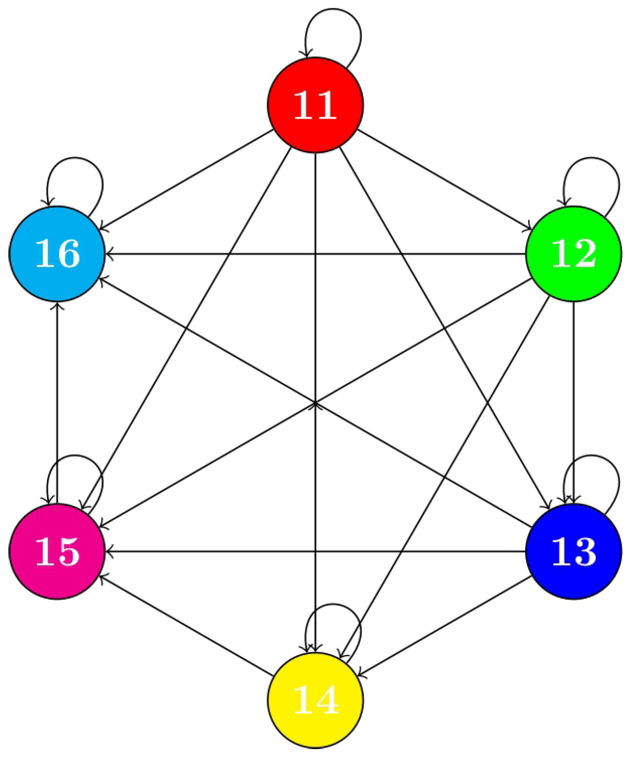
Example 4.

Let $\coprod =\{5,6,7,8,9,10,11,12\}$ and $\psi :\coprod \times \coprod \to [1,\infty )$ be a mapping such that

$$\psi (\sout{\partial },\vartheta )={\displaystyle \frac{2.58}{\sout{\partial }\vartheta +0.2}}+1.9741.$$

Consider the mapping $E_s^{\mathcal{G}}:\coprod \times \coprod \to [0,\infty )$ with the notation

$$E_s^{\mathcal{G}}(\sout{\partial },\vartheta )=\left\{\begin{array}{cc}{\left|\sout{\partial }-\vartheta \right|}^2,\hfill & if\sout{\partial }\ne \vartheta ,\hfill \\ 0,\hfill & if\sout{\partial }=\vartheta .\hfill \end{array}\right.$$

The vertex set, denoted as $\coprod =\mathbb{V}\left(\mathcal{G}\right)$, along with the specified edge set $\Xi \left(\mathcal{G}\right)$, is illustrated in Figure 3.

Clearly, $(\coprod ,E_s^{\mathcal{G}})$ is a graphically extended suprametric space but not an extended suprametric space since

$$\begin{array}{ccc}\hfill E_s^{\mathcal{G}}(10,12)& \nleqq & E_s^{\mathcal{G}}(10,11)+E_s^{\mathcal{G}}(11,12)+\psi (10,12)E_s^{\mathcal{G}}(10,11)E_s^{\mathcal{G}}(11,12).\hfill \end{array}$$

For the contractive condition, define a mapping $\Im :\coprod \to \coprod$ as

$$\Im \sout{\partial }=\left\{\begin{array}{cc}5,& for\sout{\partial }=7,\\ 6,& for\sout{\partial }\in \{6,11,12\}.\end{array}\right.$$

Case (i) For $\sout{\partial }=7$ and $\vartheta =6$, we have

$$\begin{array}{ccc}\hfill E_s^{\mathcal{G}}(\Im 7,\Im 6)& \le & {\beta }_1{E}_s^{\mathcal{G}}(7,6)+{\beta }_2{E}_s^{\mathcal{G}}(7,\Im 7)+{\beta }_3{E}_s^{\mathcal{G}}(6,\Im 6)\hfill \\ \hfill 1& \le & {\beta }_1\left(1\right)+{\beta }_2\left(4\right)+{\beta }_3\left(0\right).\hfill \end{array}$$

Case (ii) When $\sout{\partial }=7$ and $\vartheta =11$, we achieve

$$\begin{array}{ccc}\hfill E_s^{\mathcal{G}}(\Im 7,\Im 11)& \le & {\beta }_1{E}_s^{\mathcal{G}}(7,11)+{\beta }_2{E}_s^{\mathcal{G}}(7,\Im 7)+{\beta }_3{E}_s^{\mathcal{G}}(11,\Im 11)\hfill \\ \hfill 1& \le & {\beta }_1\left(16\right)+{\beta }_2\left(4\right)+{\beta }_3\left(25\right).\hfill \end{array}$$

Case (iii) When $\sout{\partial }=7$ and $\vartheta =12$, we achieve

$$\begin{array}{ccc}\hfill E_s^{\mathcal{G}}(\Im 7,\Im 12)& \le & {\beta }_1{E}_s^{\mathcal{G}}(7,12)+{\beta }_2{E}_s^{\mathcal{G}}(7,\Im 7)+{\beta }_3{E}_s^{\mathcal{G}}(12,\Im 12)\hfill \\ \hfill 1& \le & {\beta }_1\left(25\right)+{\beta }_2\left(4\right)+{\beta }_3\left(36\right).\hfill \end{array}$$

All the cases are satisfied for ${\beta }_1={\displaystyle \frac{1}{3}},$${\beta }_2={\displaystyle \frac{1}{4}},$${\beta }_3={\displaystyle \frac{1}{5}},$ where ${\beta }_1+{\beta }_2+{\beta }_3<1.$ Consequently, all the conditions outlined in Theorem 4 are satisfied, establishing that ”6” is the only fixed point of the mapping ℑ.

Figure 3. The Graphical Representation of the Vertex and Edges Sets for the Supra-Reich Contraction.

Figure 3. The Graphical Representation of the Vertex and Edges Sets for the Supra-Reich Contraction.

Definition 6.

A mapping  $\Im :\coprod \to \coprod$ is claimed as a graphical supra-Ciric contraction on the graphically extended suprametric space $(\coprod ,E_s^{\mathcal{G}})$, which is characterized by the following aspects

$\left(i\right)$

for all $\sout{\partial },\vartheta \in \coprod$ if

$$(\sout{\partial },\vartheta )\in \Xi \left(\mathcal{G}\right)\Rightarrow (\Im \sout{\partial },\Im \vartheta )\in \Xi \left(\mathcal{G}\right),$$

ensuring that ℑ preserves $\Xi \left(\mathcal{G}\right),$

$\left(ii\right)$

for all $\sout{\partial },\vartheta \in \coprod$ with $(\sout{\partial },\vartheta )\in \Xi \left(\mathcal{G}\right)$ there exists $\alpha \in (0,1)$ ensures that

$$E_s^{\mathcal{G}}\left(\Im \sout{\partial },\Im \vartheta \right)\le \alpha max\left\{E_s^{\mathcal{G}}\left(\sout{\partial },\vartheta \right),E_s^{\mathcal{G}}\left(\sout{\partial },\Im \sout{\partial }\right),E_s^{\mathcal{G}}\left(\vartheta ,\Im \vartheta \right),E_s^{\mathcal{G}}\left(\sout{\partial },\Im \vartheta \right),E_s^{\mathcal{G}}\left(\vartheta ,\Im \sout{\partial }\right)\right\}.$$

Theorem 5.

Let  $\Im :\coprod \to \coprod$ represent a self-mapping characterized as a graphical supra-Ciric contraction within a complete graphically extended suprametric space $(\coprod ,E_s^{\mathcal{G}})$. Assume that the graph $\mathcal{G}$ exhibits property $\left(\mathcal{A}\right)$. Under these conditions, there exists an element ${\sout{\partial }}_0\in \coprod$ such that $\Im \left({\sout{\partial }}_0\right)\in {\left[{\sout{\partial }}_0\right]}_{\mathcal{G}}^l$, for a certain $l\in \mathbb{N}$. Furthermore, it can be established that there exists an element ${\sout{\partial }}^{\prime }\in \coprod$, for which the sequence $\Im -PS\left\{{\sout{\partial }}_{\nu }\right\}$, is $\mathcal{G}-\mathcal{AWC}$ and converges to ${\sout{\partial }}^{\prime }$.

Proof. 

The first part of the proof follows the same structural argument presented in Theorem 1, establishing the existence of a Picard sequence ${\left\{{\sout{\partial }}_{\nu }\right\}}_{\nu \in \mathbb{N}}$ such that ${\sout{\partial }}_{\nu +1}\in {\left[{\sout{\partial }}_{\nu }\right]}_{\mathcal{G}}^l$ for all $\nu \in \mathbb{N},$ and that ${\left\{{\sout{\partial }}_{\nu }\right\}}_{\nu \in \mathbb{N}}$ is $\mathcal{G}-\mathcal{AWC}$. Utilizing the contractive condition of graphical supra-Ciric contraction, we arrive at

$$\begin{array}{c}{E}_s^{\mathcal{G}}\left({\Im }^{\nu }{\sout{\partial }}_{\rho -1},{\Im }^{\nu }{\sout{\partial }}_{\rho }\right)=E_s^{\mathcal{G}}\left(\Im \left({\Im }^{\nu -1}{\sout{\partial }}_{\rho -1}\right),\Im \left({\Im }^{\nu -1}{\sout{\partial }}_{\rho }\right)\right)\hfill \\ \\ \begin{array}{c}\le \alpha max\left\{E_s^{\mathcal{G}}\left({\Im }^{\nu -1}{\sout{\partial }}_{\rho -1},{\Im }^{\nu -1}{\sout{\partial }}_{\rho }\right),E_s^{\mathcal{G}}\left({\Im }^{\nu -1}{\sout{\partial }}_{\rho -1},\Im \left({\Im }^{\nu -1}{\sout{\partial }}_{\rho -1}\right)\right),E_s^{\mathcal{G}}\left({\Im }^{\nu -1}{\sout{\partial }}_{\rho },\Im \left({\Im }^{\nu -1}{\sout{\partial }}_{\rho }\right)\right)\right.\hfill \\ \left.E_s^{\mathcal{G}}\left({\Im }^{\nu -1}{\sout{\partial }}_{\rho -1},\Im \left({\Im }^{\nu -1}{\sout{\partial }}_{\rho -1}\right)\right),E_s^{\mathcal{G}}\left({\Im }^{\nu -1}{\sout{\partial }}_{\rho },\Im \left({\Im }^{\nu -1}{\sout{\partial }}_{\rho -1}\right)\right)\right\}\hfill \\ \\ =\alpha max\left\{E_s^{\mathcal{G}}\left({\Im }^{\nu -1}{\sout{\partial }}_{\rho -1},{\Im }^{\nu -1}{\sout{\partial }}_{\rho }\right),E_s^{\mathcal{G}}\left({\Im }^{\nu -1}{\sout{\partial }}_{\rho -1},{\Im }^{\nu -1}{\sout{\partial }}_{\rho }\right),E_s^{\mathcal{G}}\left({\Im }^{\nu -1}{\sout{\partial }}_{\rho },{\Im }^{\nu -1}{\sout{\partial }}_{\rho +1}\right)\right.\hfill \\ \left.E_s^{\mathcal{G}}\left({\Im }^{\nu -1}{\sout{\partial }}_{\rho -1},{\Im }^{\nu -1}{\sout{\partial }}_{\rho }\right),E_s^{\mathcal{G}}\left({\Im }^{\nu -1}{\sout{\partial }}_{\rho },{\Im }^{\nu -1}{\sout{\partial }}_{\rho }\right)\right\}.\hfill \end{array}\hfill \end{array}$$

Choosing the maximum value as $E_s^{\mathcal{G}}\left({\Im }^{\nu -1}{\sout{\partial }}_{\rho -1},{\Im }^{\nu -1}{\sout{\partial }}_{\rho }\right)$ results with a contradiction. So, we achieve

$$E_s^{\mathcal{G}}\left({\Im }^{\nu }{\sout{\partial }}_{\rho -1},{\Im }^{\nu }{\sout{\partial }}_{\rho }\right)\le \alpha E_s^{\mathcal{G}}\left({\Im }^{\nu -1}{\sout{\partial }}_{\rho -1},{\Im }^{\nu -1}{\sout{\partial }}_{\rho }\right).$$

Persisting with the same approach until we find

$$E_s^{\mathcal{G}}\left({\Im }^{\nu }{\sout{\partial }}_{\rho -1},{\Im }^{\nu }{\sout{\partial }}_{\rho }\right)\le {\alpha }^{\nu }{E}_s^{\mathcal{G}}\left({\sout{\partial }}_{\rho -1},{\sout{\partial }}_{\rho }\right).$$

In the light of Theorem 1, we arrive at ${\left\{{\sout{\partial }}_{\nu }\right\}}_{\nu \in \mathbb{N}}$ is a Cauchy sequence and ${\sout{\partial }}_{\nu }\to {\sout{\partial }}^{\prime }\in \coprod .$ □

Theorem 6.

If the conditions of Theorem 5 are met, and the triplet $(\coprod ,E_s^{\mathcal{G}},\Im )$ effectively demonstrates property $\left({\mathcal{A}}^{*}\right)$, it follows that ℑ confidently possesses a fixed point.

Proof. 

Theorem 5 robustly establishes that the $\Im -PS$, commencing from the initial point ${\sout{\partial }}_0$, converges not only to ${\sout{\partial }}^{\prime }$ but also to its transformed counterpart $\Im {\sout{\partial }}^{\prime }$. Given that $\mathcal{G}$ is connected either ${({\sout{\partial }}^{\prime }\mathcal{P}\Im {\sout{\partial }}^{\prime })}_{\mathcal{G}}\in \Xi \left(\mathcal{G}\right)$ or ${(\Im {\sout{\partial }}^{\prime }\mathcal{P}{v}^{\prime })}_{\mathcal{G}}\in \Xi \left(\mathcal{G}\right),$ then we arrive at

$$\begin{array}{c}{E}_s^{\mathcal{G}}\left({\sout{\partial }}^{\prime },\Im {\sout{\partial }}^{\prime }\right)\le E_s^{\mathcal{G}}\left({\sout{\partial }}^{\prime },{\sout{\partial }}_{\nu }\right)+E_s^{\mathcal{G}}\left({\sout{\partial }}_{\nu },\Im {\sout{\partial }}^{\prime }\right)+\psi \left({\sout{\partial }}^{\prime },\Im {\sout{\partial }}^{\prime }\right)E_s^{\mathcal{G}}\left({\sout{\partial }}^{\prime },{\sout{\partial }}_{\nu }\right)E_s^{\mathcal{G}}\left({\sout{\partial }}_{\nu },\Im {\sout{\partial }}^{\prime }\right)\hfill \\ \\ =E_s^{\mathcal{G}}\left({\sout{\partial }}^{\prime },{\sout{\partial }}_{\nu }\right)+E_s^{\mathcal{G}}\left(\Im {\sout{\partial }}_{\nu -1},\Im {\sout{\partial }}^{\prime }\right)+\psi \left({\sout{\partial }}^{\prime },\Im {\sout{\partial }}^{\prime }\right)E_s^{\mathcal{G}}\left({\sout{\partial }}^{\prime },{\sout{\partial }}_{\nu }\right)E_s^{\mathcal{G}}\left({\sout{\partial }}_{\nu },\Im {\sout{\partial }}^{\prime }\right).\hfill \end{array}$$

Using the definition of graphical supra-Ciric contraction, we get

$$\begin{array}{c}{E}_s^{\mathcal{G}}\left({\sout{\partial }}^{\prime },\Im {\sout{\partial }}^{\prime }\right)\le E_s^{\mathcal{G}}\left({\sout{\partial }}^{\prime },{\sout{\partial }}_{\nu }\right)\hfill \\ \\ +max\left\{E_s^{\mathcal{G}}\left({\sout{\partial }}_{\nu -1},{\sout{\partial }}^{\prime }\right),E_s^{\mathcal{G}}\left({\sout{\partial }}_{\nu -1},\Im {\sout{\partial }}_{\nu -1}\right),E_s^{\mathcal{G}}\left({\sout{\partial }}^{\prime },\Im {\sout{\partial }}^{\prime }\right),E_s^{\mathcal{G}}\left({\sout{\partial }}_{\nu -1},\Im {\sout{\partial }}^{\prime }\right),E_s^{\mathcal{G}}\left({\sout{\partial }}^{\prime },\Im {\sout{\partial }}_{\nu -1}\right)\right\}\hfill \\ \\ +\psi \left({\sout{\partial }}^{\prime },\Im {\sout{\partial }}^{\prime }\right)E_s^{\mathcal{G}}\left({\sout{\partial }}^{\prime },{\sout{\partial }}_{\nu }\right)E_s^{\mathcal{G}}\left({\sout{\partial }}_{\nu },\Im {\sout{\partial }}^{\prime }\right).\hfill \end{array}$$

Upon taking the limit as $\nu \to \infty$, we arrive at the inequality

$$E_s^{\mathcal{G}}({\sout{\partial }}^{\prime },\Im {\sout{\partial }}^{\prime })\le \alpha E_s^{\mathcal{G}}({\sout{\partial }}^{\prime },\Im {\sout{\partial }}^{\prime }),$$

which leads to a contradiction. Consequently, it follows that ${\sout{\partial }}^{\prime }$ serves as a fixed point of the mapping ℑ. □

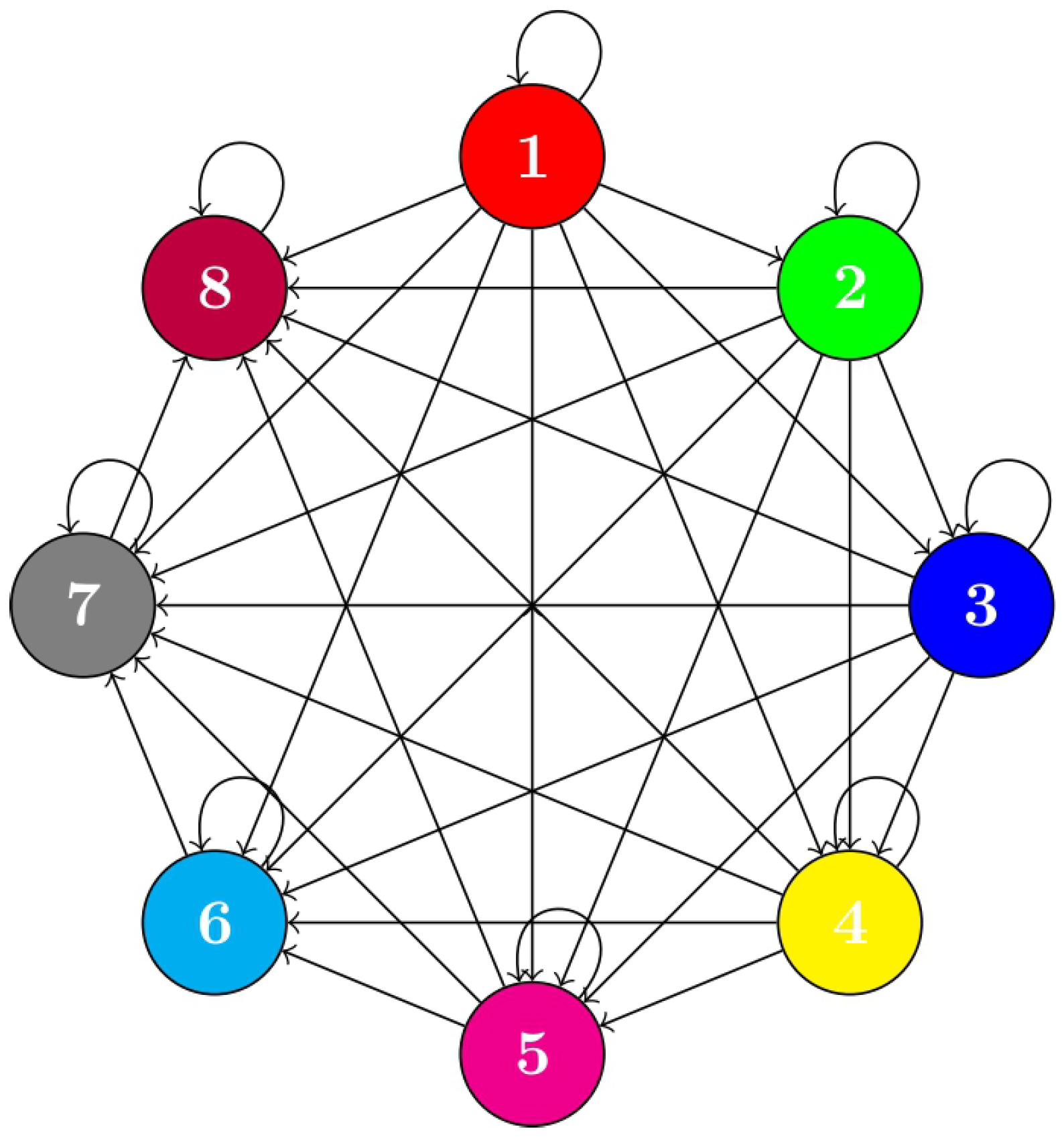
Example 5.

Let $\coprod =\{1,2,3,4,5,6,7,8\}$ and $\psi :\coprod \times \coprod \to [1,\infty )$ be a mapping such that

$$\psi (\sout{\partial },\vartheta )={\displaystyle \frac{2}{\sout{\partial }\vartheta +2}}+1.950.$$

Consider the function $E_s^{\mathcal{G}}:\coprod \times \coprod \to [0,\infty )$, referred to as

$$E_s^{\mathcal{G}}(\sout{\partial },\vartheta )=\left\{\begin{array}{cc}{\left|\sout{\partial }-\vartheta \right|}^2,\hfill & if\sout{\partial }\ne \vartheta \hfill \\ 0,\hfill & if\sout{\partial }=\vartheta .\hfill \end{array}\right.$$

The set of vertices, denoted as $\coprod =\mathbb{V}\left(\mathcal{G}\right)$, along with the corresponding edge set $\Xi \left(\mathcal{G}\right)$, is illustrated in Figure 4.

Clearly, $(\coprod ,E_s^{\mathcal{G}})$ is a graphically extended suprametric space but not an extended suprametric space, as

$$\begin{array}{ccc}\hfill E_s^{\mathcal{G}}(6,8)& \nleqq & E_s^{\mathcal{G}}(6,7)+E_s^{\mathcal{G}}(7,8)+\psi (6,8)E_s^{\mathcal{G}}(6,7)E_s^{\mathcal{G}}(7,8).\hfill \end{array}$$

For the contractive condition, define a mapping $\Im :\coprod \to \coprod$ as

$$\Im \sout{\partial }=\left\{\begin{array}{cc}2,& for\sout{\partial }=1\\ 3,& for\sout{\partial }\in \{3,6,8\}.\end{array}\right.$$

Case (i) For $\sout{\partial }=1$ and $\vartheta =3$, we have

$$\begin{array}{ccc}\hfill E_s^{\mathcal{G}}(\Im 1,\Im 3)& \le & \beta max\{E_s^{\mathcal{G}}(1,3),E_s^{\mathcal{G}}(1,\Im 1),E_s^{\mathcal{G}}(3,\Im 3),E_s^{\mathcal{G}}(1,\Im 3),E_s^{\mathcal{G}}(3,\Im 1)\},\hfill \\ \hfill 1& \le & \beta max\{4,1,0,4,1\},\hfill \\ \hfill 1& \le & \beta \left(4\right).\hfill \end{array}$$

Case (ii) If $\sout{\partial }=1$ and $\vartheta =6$, we obtain

$$\begin{array}{ccc}\hfill E_s^{\mathcal{G}}(\Im 1,\Im 6)& \le & \beta max\{E_s^{\mathcal{G}}(1,6),E_s^{\mathcal{G}}(1,\Im 1),E_s^{\mathcal{G}}(6,\Im 6),E_s^{\mathcal{G}}(1,\Im 6),E_s^{\mathcal{G}}(6,\Im 1)\},\hfill \\ \hfill 1& \le & \beta max\{25,1,9,4,16\},\hfill \\ \hfill 1& \le & \beta \left(25\right).\hfill \end{array}$$

Case (iii) If $\sout{\partial }=1$ and $\vartheta =8$, we conclude

$$\begin{array}{ccc}\hfill E_s^{\mathcal{G}}(\Im 1,\Im 8)& \le & \beta max\{E_s^{\mathcal{G}}(1,8),E_s^{\mathcal{G}}(1,\Im 1),E_s^{\mathcal{G}}(8,\Im 8),E_s^{\mathcal{G}}(1,\Im 8),E_s^{\mathcal{G}}(8,\Im 1)\},\hfill \\ \hfill 1& \le & \beta max\{49,1,25,4,36\},\hfill \\ \hfill 1& \le & \beta \left(49\right).\hfill \end{array}$$

In the subsequent discussion, it is concluded that the hypothesis of Theorem 5 holds.

Let ${\partial }_{\nu +1}=\Im \left({\partial }_{\nu }\right)$ be the Picard sequence. Typical traces are

$$1\to 2\to 3\to 3\to \dots ,4\to 1\to 2\to 3\to \dots ,$$

$$6\to 3\to 3\to \dots ,8\to 3\to 3\to \dots .$$

Since $\mathcal{G}$ is undirected complete graph with loops, $({\partial }_{\nu },{\partial }_{\nu +1})\in E\left(\mathcal{G}\right)$, so ${\partial }_{\nu +1}\in {\left[{\partial }_{\nu }\right]}_G^1$ at every step. Moreover,

$$E_s^{\mathcal{G}}({\partial }_1,{\partial }_0)\in \{1,4,9,25,36,49\},E_s^{\mathcal{G}}({\partial }_{\nu +1},{\partial }_{\nu })=0(\nu \ge 1\mathrm{once}{\partial }_{\nu }=3),$$

hence ${\sum }_{\nu \ge 0}{E}_s^{\mathcal{G}}({\partial }_{\nu +1},{\partial }_{\nu })<\infty$, that is, the Picard sequence is $\mathcal{G}$–$\mathcal{AWC}$ and converges to the unique fixed point.

It is established that all requisite conditions are fulfilled for the parameter $\beta ={\displaystyle \frac{1}{4}}$, which resides within the interval $(0,1)$. Consequently, all the criteria delineated in Theorem 6 are satisfied, affirming that “3” serves as the unique fixed point of the mapping ℑ.

3. Application to Market Dynamics

The study integrates its proposed solutions within the dynamic market equilibrium framework prevalent in economic analysis, thereby constructing a mathematical model through the resolution of an initial value problem. Both consumer and producer markets undergo substantial perturbations arising from daily price fluctuations and pricing data. Despite the inherent variability in prices, daily pricing trends exert a significant influence on the markets for production, denoted as ${\eta }_{\tau }$, and consumption, represented as ${\eta }_{\mathfrak{c}}$. Throughout this economic analysis, the economist endeavors to ascertain the current price, expressed mathematically as $\hslash \left(\rho \right)$.

We define the pair ${\eta }_{\tau }$ and ${\eta }_{\mathfrak{c}}$ by the system

$$\begin{array}{ccc}\hfill {\eta }_{\tau }& =& t_1+{\xi }_1\hslash \left(\rho \right)+{\delta }_1{\displaystyle \frac{d\hslash \left(\rho \right)}{d\rho }}+{\sigma }_1{\displaystyle \frac{d^2\hslash \left(\rho \right)}{d{\rho }^2}},\hfill \\ \\ \hfill {\eta }_c& =& t_2+{\xi }_2\hslash \left(\rho \right)+{\delta }_2{\displaystyle \frac{d\hslash \left(\rho \right)}{d\rho }}+{\sigma }_2{\displaystyle \frac{d^2\hslash \left(\rho \right)}{d{\rho }^2}},\hfill \end{array}$$

subject to

$$\hslash \left(0\right)=0,{\displaystyle \frac{d\hslash }{d\rho }}\left(0\right)=0,$$

where $t_1,t_2,{\xi }_1,{\xi }_2,{\delta }_1,{\delta }_2,{\sigma }_1$ and ${\sigma }_2$ are constants.

A state of dynamic economic equilibrium is achieved when market forces reach a state of equilibrium, indicating that the disparity between production and consumption has stabilized. In this condition, the elasticity of supply, denoted as ${\eta }_{\tau }$, is equal to the elasticity of demand, represented as ${\eta }_c$. Hence

$$\begin{array}{ccc}\hfill t_1+{\xi }_1\hslash \left(\rho \right)+{\delta }_1{\displaystyle \frac{d\hslash \left(\rho \right)}{d\rho }}+{\sigma }_1{\displaystyle \frac{d^2\hslash \left(\rho \right)}{d{\rho }^2}}& =& t_2+{\xi }_1\hslash \left(\rho \right)+{\delta }_2{\displaystyle \frac{d\hslash \left(\rho \right)}{d\rho }}+{\sigma }_2{\displaystyle \frac{d^2\hslash \left(\rho \right)}{d{\rho }^2}},\hfill \\ \\ \hfill \left(t_1-t_2\right)+\left({\xi }_1-{\xi }_2\right)\hslash \left(\rho \right)& +& \left({\delta }_1-{\delta }_2\right){\displaystyle \frac{d\hslash \left(\rho \right)}{d\rho }}+\left({\sigma }_1-{\sigma }_2\right){\displaystyle \frac{d^2\hslash \left(\rho \right)}{d{\rho }^2}}=0,\hfill \\ \\ \hfill \sigma {\displaystyle \frac{d^2\hslash \left(\rho \right)}{d{\rho }^2}}+\delta {\displaystyle \frac{d\hslash \left(\rho \right)}{d\rho }}+\xi \nu \left(\rho \right)& =& -t,\hfill \\ \\ \hfill {\displaystyle \frac{d^2\hslash \left(\rho \right)}{d{\rho }^2}}+{\displaystyle \frac{\delta }{\sigma }}{\displaystyle \frac{d\hslash \left(\rho \right)}{d\rho }}+{\displaystyle \frac{\xi }{\sigma }}\hslash \left(\rho \right)& =& -{\displaystyle \frac{t}{\sigma }},\hfill \end{array}$$

where $t=t_1-t_2,\xi ={\xi }_1-{\xi }_2,\delta ={\delta }_1-{\delta }_2$, and $\sigma ={\sigma }_1-{\sigma }_2$.

The initial value problem can be articulated in the following manner

$${\hslash }^{\prime \prime }\left(\rho \right)+{\displaystyle \frac{\delta }{\sigma }}{\hslash }^{\prime }\left(\rho \right)+{\displaystyle \frac{\xi }{\sigma }}\hslash \left(\rho \right)=-{\displaystyle \frac{t}{\sigma }},\mathrm{with}\hslash \left(0\right)=0\mathrm{and}{\hslash }^{\prime }\left(0\right)=0.$$

(1)

In the present analysis, we examine the duration of production and consumption, denoted as $\omega$. It is established that the problem represented by Equation (1) corresponds equivalently to

$$\hslash \left(\rho \right)={\int }_0^{\omega }\mathcal{G}\left(\rho ,{\rho }^{*}\right)\mathcal{K}\left({\rho }^{*},\rho ,\hslash \left(\rho \right)\right)d\rho ,$$

(2)

where Green’s function $\mathcal{G}\left(\rho ,{\rho }^{*}\right)$ is

$$\mathcal{G}\left(\rho ,{\rho }^{*}\right)=\left\{\begin{array}{cc}\rho {exp}^{{\displaystyle \frac{\xi }{2n}}}\left({\rho }^{*}-\rho \right);\hfill & 0\le \rho \le \mathfrak{s}\le \omega \hfill \\ \mathfrak{s}{exp}^{{\displaystyle \frac{\xi }{2\eta }}}\left(\rho -{\rho }^{*}\right);\hfill & 0\le \mathfrak{s}\le \rho \le \omega ,\hfill \end{array}\right.$$

and $\mathcal{K}:[0,\omega ]\times {\mathbb{V}}^2\to \mathbb{R}$ is a continuous function.

Let $\coprod =\mathcal{C}\left(\right[0,\omega ],\mathbb{R})$ and define the metric as

$$E_s^{\mathcal{G}}(\hslash \left(\rho \right),\mu \left(\rho \right))=\underset{\rho \in [0,1]}{sup}{|\hslash \left(\rho \right)-\mu \left(\rho \right)|}^2$$

with $\psi (\hslash \left(\rho \right),\mu \left(\rho \right))={exp}^{\hslash \left(\rho \right)+\mu \left(\rho \right)}$ and for all $(\hslash ,\mu )\in \Xi \left(\mathcal{G}\right)$. Employing this metric, we establish that $(\coprod ,E_s^{\mathcal{G}})$ qualifies as a complete graphical extended suprametric space. Define the mapping $\Im :\coprod \to \coprod$ by the following equation

$$\Im (\hslash \left(\rho \right))={\int }_0^{\omega }\mathcal{G}\left(\rho ,{\rho }^{*}\right)\mathcal{K}\left({\rho }^{*},\rho ,\hslash \left(\rho \right)\right)d\rho .$$

(3)

To explore the resolution of the dynamic market equilibrium problem, we can assert that the solution, denoted in Equation (1), serves as a fixed point of the operator ℑ.

Theorem 7.

Consider the operator $\Im :\coprod \to \coprod$, which satisfies the subsequent features:

$\left(i\right)$

there exists a $\rho \in [0,\omega ]$ such that

$$\left|\mathcal{K}\left({\rho }^{*},\rho ,{\hslash }_1\left(\rho \right)\right)-\mathcal{K}\left({\rho }^{*},\rho ,{\hslash }_2\left(\rho \right)\right)\right|\le \sqrt{{\beta }_1{\left|{\hslash }_1\left(\rho \right)-{\hslash }_2\left(\rho \right)\right|}^2+{\beta }_2{\left|{\hslash }_1\left(\rho \right)-\Im {\hslash }_1\left(\rho \right)\right|}^2+{\beta }_3{\left|{\hslash }_2\left(\rho \right)-\Im {\hslash }_2\left(\rho \right)\right|}^2};$$

$\left(ii\right)$

there is a continuous function $\mathcal{G}:{\mathbb{V}}^2\to \mathbb{R}$ that holds the property

$$\underset{\mathfrak{s}\in [0,\omega ]}{sup}{\int }_0^{\omega }\mathcal{G}\left(\rho ,{\rho }^{*}\right)d\rho \le 1.$$

Consequently, the dynamic market equilibrium problem delineated in Equation (1) possesses a unique solution.

Proof. 

It is evident that the function ℑ is well-defined, and we can assert the subsequent statement

$$\begin{array}{cc}\hfill \left|\Im \left({\hslash }_1\left(\rho \right)\right)-\Im \left({\hslash }_2\left(\rho \right)\right)\right|& =\left|{\int }_0^{\omega }\mathcal{G}\left(\rho ,{\rho }^{*}\right)\mathcal{K}\left({\rho }^{*},\rho ,{\hslash }_1\left(\rho \right)\right)d\rho -{\int }_0^{\omega }\mathcal{G}\left(\rho ,{\rho }^{*}\right)\mathcal{K}\left({\rho }^{*},\rho ,{\hslash }_2\left(\rho \right)\right)d\rho \right|\hfill \\ & \le {\int }_0^{\omega }\mathcal{G}\left(\rho ,{\rho }^{*}\right)d\rho {\int }_0^{\omega }\left|\mathcal{K}\left({\rho }^{*},\rho ,{\hslash }_1\left(\rho \right)\right)-\mathcal{K}\left({\rho }^{*},\rho ,{\hslash }_2\left(\rho \right)\right)\right|d\rho \hfill \\ & \le \sqrt{{\beta }_1{\left|{\hslash }_1\left(\rho \right)-{\hslash }_2\left(\rho \right)\right|}^2+{\beta }_2{\left|{\hslash }_1\left(\rho \right)-\Im {\hslash }_1\left(\rho \right)\right|}^2+{\beta }_3{\left|{\hslash }_2\left(\rho \right)-\Im {\hslash }_2\left(\rho \right)\right|}^2}.\hfill \end{array}$$

Consider the following inequality derived by squaring both sides of the expression

$$|\Im {\hslash }_1\left(\rho \right)-\Im {\hslash }_2{\left(\rho \right)|}^2\le {\beta }_1{\left|{\hslash }_1\left(\rho \right)-{\hslash }_2\left(\rho \right)\right|}^2+{\beta }_2{\left|{\hslash }_1\left(\rho \right)-\Im {\hslash }_1\left(\rho \right)\right|}^2+{\beta }_3{\left|{\hslash }_2\left(\rho \right)-\Im {\hslash }_2\left(\rho \right)\right|}^2,$$

that can be expressed as

$$E_s^{\mathcal{G}}(\Im {\hslash }_1\left(\rho \right),\Im {\hslash }_2\left(\rho \right))\le {\beta }_1{E}_s^{\mathcal{G}}({\hslash }_1\left(\rho \right),{\hslash }_2\left(\rho \right))+{\beta }_2{E}_s^{\mathcal{G}}({\hslash }_1\left(\rho \right),\Im {\hslash }_1\left(\rho \right))+{\beta }_3{E}_s^{\mathcal{G}}({\hslash }_2\left(\rho \right),\Im {\hslash }_2\left(\rho \right)).$$

Under the fulfillment of all conditions indicated in Theorem 3, it can be concluded that the integral Equation (2) possesses a unique solution. Consequently, this implies that the dynamic market equilibrium problem delineated in (1) also exhibits a unique solution. □

4. Numerical Approximation of the Integral Equation

To numerically validate the theoretical results obtained in Theorem 3, we solve the nonlinear integral equation

$$\hslash \left(\rho \right)={\int }_0^w\mathcal{G}(\rho ,{\rho }^{*})\mathcal{K}({\rho }^{*},\rho ,\hslash \left(\rho \right))d{\rho }^{*},$$

using a successive approximation scheme that is Picard iteration. The function $\hslash \left(\rho \right)$ models the price evolution under the influence of dynamic production and consumption changes.

For the numerical experiment, we consider a simplified model where the Green’s function is given by

$$\mathcal{G}(\rho ,{\rho }^{*})=\left\{\begin{array}{cc}\rho exp\left({\displaystyle \frac{\xi }{2}}({\rho }^{*}-\rho )\right),\hfill & if\rho \le {\rho }^{*},\hfill \\ {\rho }^{*}exp\left({\displaystyle \frac{\xi }{2}}(\rho -{\rho }^{*})\right),\hfill & if\rho >{\rho }^{*},\hfill \end{array}\right.$$

with $\xi =2.0$, the nonlinear kernel is defined as $\mathcal{K}({\rho }^{*},\rho ,\hslash )=sin(\hslash )+{\rho }^{*}\rho$, initial guess: ${\hslash }_0\left(\rho \right)\equiv 0$, convergence tolerance: ${10}^{-6}$, and discretization: 100 uniform points over the interval $[0,1]$.

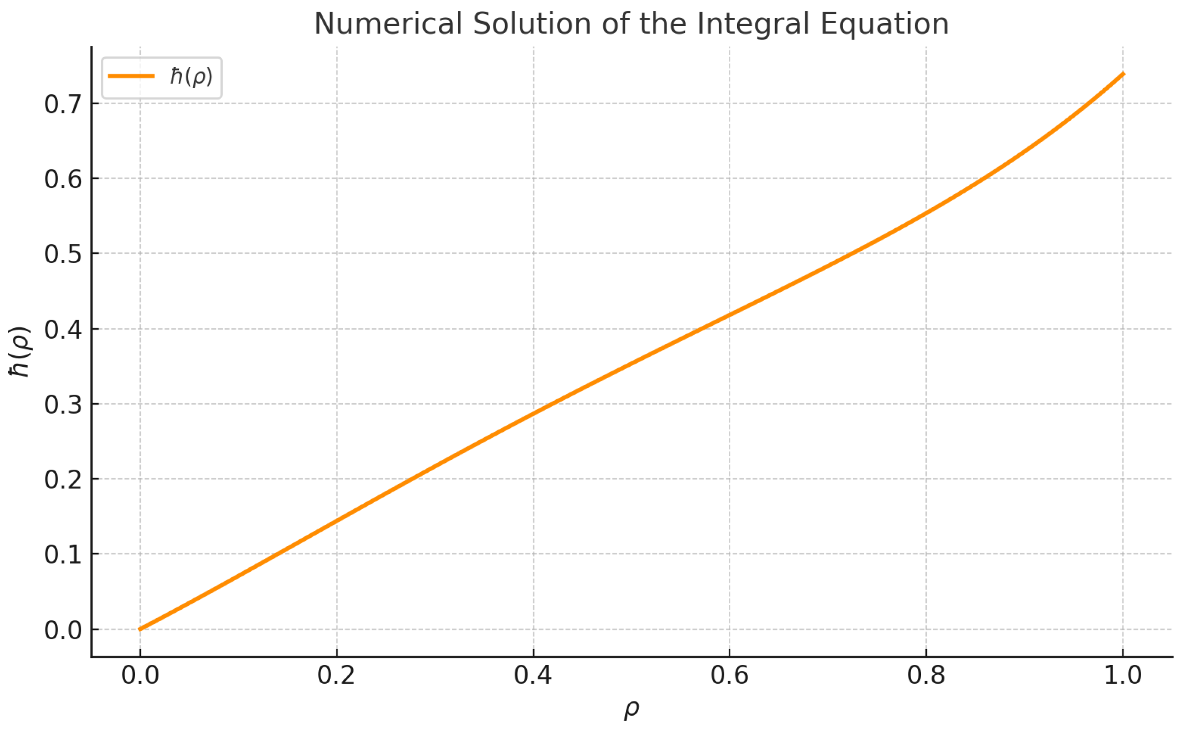
After iterative computation, the solution $\hslash \left(\rho \right)$ converges to a stable trajectory. The figure below illustrates the final result.

This result numerically confirms the existence and uniqueness of the fixed point in the graphically extended suprametric setting, thereby validating the analytical framework proposed in this study.

Classical fixed-point formulations, such as those based on Banach’s contraction principle, typically operate in complete metric or normed spaces and rely on global contraction conditions:

$$d(\Im \sout{\partial },\Im \vartheta )\le \lambda d(\sout{\partial },\vartheta ),\lambda \in (0,1),$$

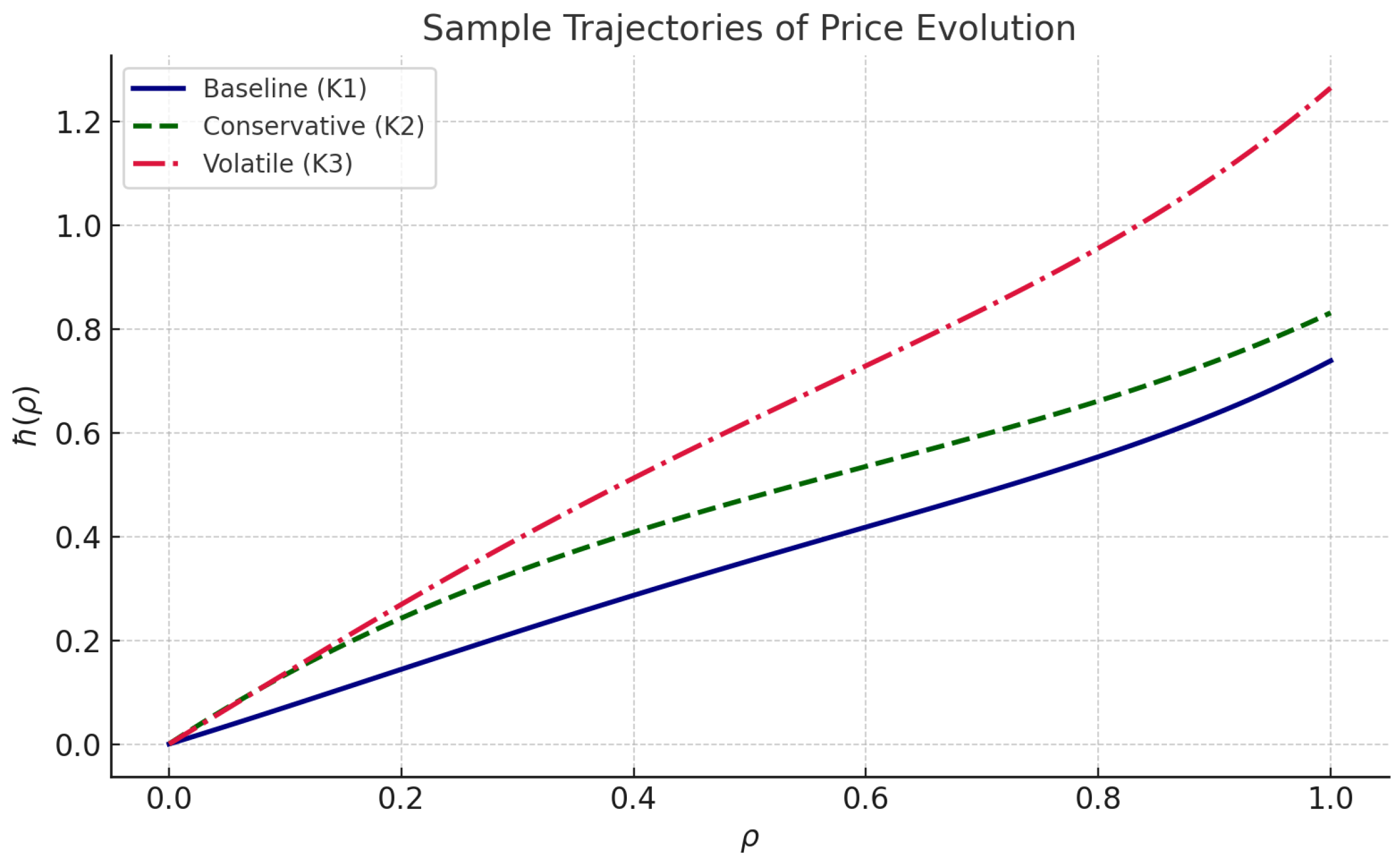
ensuring convergence of iterates to a unique fixed point. While powerful, this approach assumes a homogeneous structure and full domain interaction, which may not accurately represent dynamic systems with localized or constrained dependencies such as production consumption feedback loops in economic networks. The numerical behaviour of the iterative solution, showing the convergence of the Picard iteration and the corresponding price change biases, is illustrated in Figure 5 and Figure 6.

In contrast, our model utilizes a graphically extended suprametric space, denoted by $(\coprod ,E_s^{\mathcal{G}})$, where the metric is enriched by

• Localized connectivity via a directed graph $\mathcal{G}$,
• A modified triangle inequality involving a kernel function $\psi (\sout{\partial },\vartheta )$,
• Structural flexibility allowing asymmetric and nonlinear feedback mechanisms.

This generalized setting enables more realistic modeling of dynamic markets where not all variables interact symmetrically or globally. For example, certain agents such as producers or consumers may only influence subsets of the system, and information may propagate through sparse or hierarchical channels. The suprametric graph captures such nuances through its edge structure and allows path-dependent convergence properties.

Additionally, graphical contractions for instance supra-Kannan, supra-Reich, supra-Ciric provide more relaxed fixed-point conditions compared to Banach’s model, admitting convergence even when traditional global contraction is not satisfied. This is particularly relevant for systems with delayed feedback or response lags, topological constraints such as supply-chain bottlenecks, and varying node influence in price or production adjustments.

Overall, the incorporation of graphically extended suprametrics not only generalizes classical results but also aligns better with network-driven equilibrium dynamics, offering both theoretical richness and application potential in nonlinear economic systems.

5. Broader Impacts and Future Applicability

The framework of graphically extended suprametric spaces developed in this study offers promising avenues for application beyond traditional equilibrium models, particularly in the analysis of decentralized, interconnected, or intelligent systems. In modern economic ecosystems such as energy trading platforms, logistics supply chains, or financial networks, agents are interconnected through dynamic, often asymmetric, relationships. Graph-based suprametric structures allow for modeling:

• localized dependencies (e.g., regional price coupling),
• heterogeneous agent roles (e.g., dominant suppliers vs. fringe actors),
• and time-lagged interactions (e.g., delivery, inventory adjustment).

These models can capture the cascading and nonlinear feedback effects that emerge in real-world economic networks far more effectively than classical global metric-based models.

In online platforms (e.g., gig economies, e-commerce, advertising auctions), participants are matched dynamically under partial information and algorithmic pricing. The graph structure can encode digital trust, transaction history, or algorithmic recommendations. Suprametric modeling allows for

• personalized equilibrium pricing,
• adaptive contract design,
• and platform-wide stability analysis under user churn or market shocks.

Autonomous agents in AI-based systems such as collaborative robots, distributed optimization, or federated learning operate within structured interaction graphs. The proposed fixed point framework enables:

• formal guarantees of convergence in asynchronous or partially connected systems,
• sensitivity control through the kernel $\psi$,
• and design of decentralized coordination rules.

Future work could integrate stochastic graph evolution, dynamic node behavior, and real-time control into the suprametric structure, enabling truly adaptive systems analysis. This will bridge the gap between mathematical rigor and engineering-scale implementation across economics, digital infrastructures, and AI.

6. Illustrative Economic Application: Inflation Dynamics in Commodity Networks

To demonstrate the practical relevance of the proposed graphical suprametric model, consider its application to inflation modeling across a multi-tier commodity network. In such a system, producers, suppliers, and distributors are interlinked in a directed graph structure $\mathcal{G}=(\mathbb{V},\Xi )$, where each node $v\in \mathbb{V}$ corresponds to a market agent or sector for instance agriculture, transport, retail, and edges encode transactional influence.

Suppose inflation pressure at a node $\rho$ depends nonlinearly on both its own past inflation rate and aggregated influence from connected suppliers. This can be captured by a fixed-point formulation

$$\hslash \left(\rho \right)={\int }_0^1\mathcal{G}(\rho ,{\rho }^{*})·\mathcal{K}({\rho }^{*},\rho ,\hslash \left({\rho }^{*}\right))d{\rho }^{*},$$

where $\hslash \left(\rho \right)$ denotes the local inflation rate at market node $\rho$, $\mathcal{G}$ reflects the directional impact of upstream nodes such as cost-push inflation, and $\mathcal{K}$ is a nonlinear kernel encoding behavioral or policy responses.

This structure naturally accommodates with

• Inflationary propagation through commodity chains,
• Localized shocks (e.g., oil price spikes, wage contracts),
• Delayed or asymmetric interactions between sectors,
• Policy interventions as perturbations to the kernel function.

Thus, the suprametric fixed-point formulation provides a mathematically robust and interpretively rich framework for studying inflation stabilization, price diffusion, or multi-sector equilibrium evolution in complex economies.

The convergence of the Picard iteration can be effectively illustrated through the construction of a small weighted graph. The following example will serve to demonstrate the iterative process and its trajectory toward a fixed point, ultimately highlighting the reliability of the method in producing consistent solutions.

Example 6.

Let $\coprod =[0,1]$ and equip it with the undirected complete graph $\mathcal{G}$ (all loops $(\sout{\partial },\sout{\partial })$ and all directed edges $(\sout{\partial },\vartheta )$). Define $E_s^{\mathcal{G}}(\sout{\partial },\vartheta )=|\sout{\partial }-\vartheta |$ and $\psi (\sout{\partial },\vartheta )\equiv 1$. Consider the self-map $\Im :\coprod \to \coprod$ given by $\Im \left(\sout{\partial }\right)=0.6x+0.16$; then $\Im (\coprod )\subset [0.16,0.76]\subset \coprod$.

For all $\sout{\partial },\vartheta \in \coprod$,

$$\begin{array}{cc}\hfill E_s^{\mathcal{G}}(\Im \sout{\partial },\Im \vartheta )& =0.6|\sout{\partial }-\vartheta |\hfill \\ \hfill & \le \alpha E_s^{\mathcal{G}}(\sout{\partial },\vartheta )\le \alpha max\left\{E_s^{\mathcal{G}}(\sout{\partial },\vartheta ),E_s^{\mathcal{G}}(\sout{\partial },\Im \sout{\partial }),E_s^{\mathcal{G}}(\vartheta ,\Im \vartheta ),E_s^{\mathcal{G}}(\sout{\partial },\Im \vartheta ),E_s^{\mathcal{G}}(\vartheta ,\Im \sout{\partial })\right\},\hfill \end{array}$$

with $\alpha =0.6\in (0,1)$. Hence ℑ is a graphical supra-Ciric contraction where the edge preservation is trivial since G is complete. The Picard iteration ${\sout{\partial }}_{n+1}=\Im {\sout{\partial }}_n$ starting from ${\sout{\partial }}_0=1$ is

$${\sout{\partial }}_1=0.76,{\sout{\partial }}_2=0.616,{\sout{\partial }}_3=0.5296,{\sout{\partial }}_4=0.47776,\dots$$

and admits the closed form ${\sout{\partial }}_n=0.4+0.6^n({\sout{\partial }}_0-0.4)$, hence converges geometrically to the unique fixed point ${\sout{\partial }}^{*}=0.4$ solving ${\sout{\partial }}^{*}=0.6x^{*}+0.16$.

7. Conclusions

This research investigation delves into the realm of graphically extended suprametric spaces, effectively merging the theoretical constructs of suprametric space theory with graphical structures. By introducing and rigorously analyzing graphical supra-Kannan, supra-Reich, and supra-Ciric contractions, we have successfully established both the existence and uniqueness of fixed points for these mappings within complete graphically extended suprametric spaces. Our findings serve to generalize and extend prior contributions to fixed point theory, showcasing the enhanced versatility and applicability of graphical structures within this mathematical context.

The illustrative examples provided within this paper elucidate the practical utility of our theoretical framework, demonstrating how the incorporation of graphical features can significantly enrich the traditional understanding of suprametric spaces. Furthermore, our application of these concepts to dynamic market equilibrium exemplifies the relevance of our results in tackling real-world problems, particularly within the domains of economic modeling and analysis.

Open Problems and Future Directions

• A promising area for further exploration includes the investigation of fixed point existence for alternative types of graphical contractions, such as supra-Ćirić-Reich-Rus or supra-Hardy-Rogers contractions, within the context of graphically extended suprametric spaces.
• Future research could also extend the established results to encompass multivalued mappings, examining their implications and applications within optimization and control theory.
• The application of graphically extended suprametric spaces to network analysis represents a compelling direction for research, particularly in studying aspects of connectivity and stability within complex systems.
• The formulation of numerical algorithms grounded in the fixed point theorems presented in this work could be pivotal in addressing nonlinear equations that arise across engineering and economics.

This work opens new avenues for research in fixed point theory and its applications, bridging the gap between abstract mathematical structures and practical problems. Subsequent investigations may further refine these theoretical concepts and uncover their potential in a multitude of interdisciplinary contexts.