Moment Estimation for Uncertain Delay Differential Equations via the Composite Heun Scheme

Abstract

As an important mathematical model actuated by the Liu process, uncertain delay differential equations depict the development of system dynamics. In the applications of uncertain delay differential equations, parameter estimation plays a key role. In the paper, a new scheme called the composite Heun scheme is introduced. This scheme is then incorporated into the method of moments to estimate the unknown parameters in uncertain delay differential equations. Some numerical examples are given to illustrate the feasibility of the composite Heun scheme. Two distinct types of uncertain delay differential equations with integer delay time and noninteger delay time are discussed. Finally, we present an uncertain delay stock model to forecast the stock prices of Xiamen Airlines by using the parameter estimation approach proposed in this work.

1. Introduction

Continuous time processes involving some time delay are widespread in many areas. The delay differential equations are usually applied to model the automatic control systems, such as population dynamics [1], tumor growth [2], and chemical kinetics [3], etc. In effect, the dynamical systems are often disturbed by random noise, and the rate of temporal change is contingent on the current and past state of the system. In this case, to describe and analyze these systems, stochastic delay differential equations, which include time delay terms, are devised. Since then, stochastic delay differential equations have been broadly used in many domains, like logistic models [4], finance [5], genetic regulatory networks [6], and the optimal control problem [7].

Although there is a comprehensive study of stochastic delay differential equations, it is considered under the framework of probability theory. The resulting distribution function must be sufficiently near to the real frequency in order for probability theory to make sense. Nevertheless, we frequently have to rely on the belief degree provided by certain professors, and the range of belief degree is much larger than the actual frequency [8]. In addition, numerous time-varying systems may not be successfully simulated using stochastic delay differential equations when Wiener processes are used to describe white noise. Other approaches are therefore required to characterize dynamic systems with noise. In order to cope with general uncertainty, Liu [9] established the uncertainty theory, which is a branch of mathematics based on normality, duality, subadditivity, and product axioms. To better simulate the uncertain phenomenon of time change, Liu [10] defined the notion of the uncertainty process. A sample Lipschitz consecutive uncertain process with steady independent increments is known as the Liu process [10], which is characterized by stationary independent increments that follow an uncertain normal distribution. Delay differential equations take into account the temporal memory effect of systems, which makes them more efficient in representing many natural phenomena [11,12]. In response to the uncertain kinetic system, uncertain differential equations actuated by the Liu process were first proposed by Liu [13]. By means of the Liu process, Barbacioru [14] proposed uncertain delay differential equations and initially presented a local existence and uniqueness solution for a particular kind of uncertain delay differential equation. Afterwards, Ge and Zhu [15] testified an existence and uniqueness theorem of solution for uncertain delay differential equations under Lipschitz conditions and linear growth conditions in accordance with Banach’s immovable point theorem. Moreover, Wang and Ning [16] studied the measure stability, mean stability, moment stability and the interconnections among them. Jia and Sheng [17] also explored the stability in distribution for uncertain delay differential equations and established a sufficient condition for being stable in distribution.

In uncertain delay differential equations, there are parameters that are unknown. Therefore, how to estimate these parameters by means of observation is a critical issue. According to the Euler scheme, Yao and Liu [18] first employed the method of moments to estimate the parameters in the uncertain differential equations. Since then, various estimation methods by the Euler method have been extensively studied. Liu [19] presented the generalized moment estimation method. Then, Yao et al. [20] used the method to estimate the unknown parameters in multi-dimensional uncertain differential equations. The least squares estimation methods were explored by Sheng et al. [21]. Subsequently, Liu and Jia [22] used the moment method for the analysis of uncertain delay differential equations. Gao et al. [23] designated the value of the unknown delay time as the approximation provided by the first-order Taylor expansion. Then based on the moment estimation, the estimated parameters and the delay time were obtained. Afterwards, Li and Xia [24] proposed an estimating function technique based on function expansion to estimate the parameters in uncertain differential equations. However, when we cope with some nonparametric uncertain differential equations, the parameter estimation method may not be used directly. Therefore, He et al. [25] deduced the method of nonparametric estimation for autonomous uncertain differential equations and applied it to a carbon dioxide model. Then, He and Zhu [26] applied the method to uncertain fractional differential equations and the error analysis of this method was given.

Nevertheless, the Euler scheme is a relatively simple difference scheme to approximate uncertain differential equations. For the sake of enhancing the precision of approximation, Zhou et al. [27] deduced the composite Heun scheme. Then the composite Heun scheme was successfully applied to the method of moments to estimate the parameters in uncertain differential equations. In this paper, we study the problem of parameter estimation for uncertain delay differential equations based on the composite Heun scheme. The composite Heun scheme is extended to approximate uncertain delay differential equations. Then the unknown parameters of two different types of uncertain delay differential equations are estimated by the method of moments. We also present an uncertain delay stock model and apply it to simulate and forecast real stock prices.

The remainder of the article is arranged as follows. Section 2 presents the method of moments via the composite Heun scheme for uncertain delay differential equations with integer delay time. The composite Heun scheme is applied to parameter estimation for uncertain delay differential equations with noninteger time delay in Section 3. Section 4 provides some numerical examples to demonstrate the feasibility of the composite Heun scheme. Section 5 proposes an uncertain delay stock model for modeling the closing price of MF (the code of Xiamen Airlines named by the International Air Transport Association) stock. Finally, some concluding sentences are provided in Section 6.

2. Parameter Estimation for Uncertain Delay Differential Equations with Integer Delay Time

Suppose an uncertain process $X_t$ satisfies the following uncertain delay differential equation [14]

$$\left\{\begin{array}{c}d{X}_t=f\left(t,X_t,X_{t-\tau };\mathit{\mu }\right)dt+g\left(t,X_t,X_{t-\tau };\mathit{\mu }\right)d{C}_t,0⩽t⩽T,\hfill \\ X_t=\phi \left(t\right),-\tau ⩽t⩽0,\hfill \end{array}\right.$$

(1)

where f and g are the drift and diffusion terms that are given continuously differentiable functions and satisfy the Lipschitz condition and linear growth conditions, $\mathit{\mu }$ represents a vector containing K unknown parameters that need to be estimated, $\phi \left(t\right)$ is a initial function, $\tau >0$ is the given delay time, and $C_t$ is a Liu process. For a positive integer m, the step size h satisfies $\tau =mh$. Given a partition of the interval $[0,T]$ with $0=t_0<t_1<\dots <t_N⩽T$ where $t_{n+1}-t_n=h,$ $n=0,1,\dots ,N-1.$ According to the Heun scheme for the uncertain differential equation proposed by Zhou et al. [27], the Heun difference form of Equation (1) is

$$\left\{\begin{array}{c}{X}_{t_{n+1}}=X_{t_n}+{\displaystyle \frac{h}{2}}\left(f(t_n,X_{t_n},X_{t_{n-m}};\mathit{\mu })+f\left(t_{n+1},X_{t_n}+hf(t_n,X_{t_n},X_{t_{n-m}};\mathit{\mu }),X_{t_{n-m+1}};\mathit{\mu }\right)\right)\hfill \\ +g(t_n,X_{t_n},X_{t_{n-m}};\mathit{\mu })(C_{t_{n+1}}-C_{t_n}),0⩽n⩽N-1,\hfill \\ X_{t_{n-m}}=\phi \left(t_{n-m}\right),n-m⩽0.\hfill \end{array}\right.$$

(2)

More generally, the corresponding composite Heun scheme is

$$\left\{\begin{array}{c}{X}_{t_{n+1}}=X_{t_n}+h\left((1-\theta )f(t_n,X_{t_n},X_{t_{n-m}};\mathit{\mu })+\theta f\left(t_{n+1},X_{t_n}+hf(t_n,X_{t_n},X_{t_{n-m}};\mathit{\mu }),X_{t_{n-m+1}};\mathit{\mu }\right)\right)\hfill \\ +g(t_n,X_{t_n},X_{t_{n-m}};\mathit{\mu })(C_{t_{n+1}}-C_{t_n}),0⩽n⩽N-1,\hfill \\ X_{t_{n-m}}=\phi \left(t_{n-m}\right),n-m⩽0,\hfill \end{array}\right.$$

(3)

where $\theta$∈$[0,1]$ is a relaxation parameter. If $\theta ={\displaystyle \frac{1}{2}}$, the composite Heun scheme (3) reduces to the Heun scheme (2). Since $X_t$ is a uncertain process, the uncertain measure of $g(t_n,X_{t_n},X_{t_{n-m}};\mathit{\mu })=0$ is zero, i.e., $\mathcal{M}\left\{g(t_n,X_{t_n},X_{t_{n-m}};\mathit{\mu })=0\right\}=0$. Therefore, according to the first equation in Equation (3), we obtain

$$\begin{array}{c}\hfill {\displaystyle \frac{X_{t_{n+1}}-X_{t_n}-h(1-\theta )f(t_n,X_{t_n},X_{t_{n-m}};\mathit{\mu })-h\theta f(t_{n+1},X_{t_n}+hf(t_n,X_{t_n},X_{t_{n-m}};\mathit{\mu }),X_{t_{n-m+1}};\mathit{\mu })}{g(t_n,X_{t_n},X_{t_{n-m}};\mathit{\mu })h}}\end{array}={\displaystyle \frac{C_{t_{n+1}}-C_{t_n}}{h}}.$$

From the definition of the Liu process, we know

$$\begin{array}{c}\hfill {\displaystyle \frac{C_{t_{n+1}}-C_{t_n}}{h}}\sim \mathcal{N}(0,1).\end{array}$$

Consequently,

$$\begin{array}{c}\hfill {\displaystyle \frac{X_{t_{n+1}}-X_{t_n}-h(1-\theta )f(t_n,X_{t_n},X_{t_{n-m}};\mathit{\mu })-h\theta f(t_{n+1},X_{t_n}+hf(t_n,X_{t_n},X_{t_{n-m}};\mathit{\mu }),X_{t_{n-m+1}};\mathit{\mu })}{g(t_n,X_{t_n},X_{t_{n-m}};\mathit{\mu })h}}\sim \mathcal{N}(0,1).\end{array}$$

Suppose that there are N + 1 observation data x_t0, x_t1, …, x_tN of X_t at the times t₀, t₁, …, t_N, Replacing X_tn with the observations x_tn, we have

$$\begin{array}{c}\hfill \begin{array}{c}\hfill l_n\left(\mathit{\mu }\right)={\displaystyle \frac{x_{t_{n+1}}-x_{t_n}-h(1-\theta )f(t_n,x_{t_n},x_{t_{n-m}};\mathit{\mu })-h\theta f(t_{n+1},x_{t_n}+hf(t_n,x_{t_n},x_{t_{n-m}};\mathit{\mu }),x_{t_{n-m+1}};\mathit{\mu })}{g(t_n,x_{t_n},x_{t_{n-m}};\mathit{\mu })h}},\end{array}\end{array}$$

(4)

where n = 0, 1, …, N − 1, which can be considered as a function of the unknown parameter vector $\mathit{\mu }$. Then l₀($\mathit{\mu }$), l₁($\mathit{\mu }$), …, l_N−1($\mathit{\mu }$) can also be seen as N samples of $\mathcal{N}$(0, 1). Therefore, we can acquire the k-th sample moments

$$\begin{array}{c}\hfill {\displaystyle \frac{1}{N}}{\displaystyle \sum _{n=0}^{N-1}}{\left(l_n\left(\mathit{\mu }\right)\right)}^k,k=1,2,\dots ,\end{array}$$

and the k-th population moments

$$\begin{array}{c}\hfill {\displaystyle {\int }_0^1}{\left({\mathsf{\Phi }}^{-1}\left(\alpha \right)\right)}^{k}d\alpha ={\left({\displaystyle \frac{\sqrt{3}}{\pi }}\right)}^k{\displaystyle {\int }_0^1}{\left(ln{\displaystyle \frac{\alpha }{1-\alpha }}\right)}^{k}d\alpha =3^{{\displaystyle \frac{k}{2}}}(2^k-2)\left|B_k\right|,k=1,2,\dots ,\end{array}$$

where Φ⁻¹(α) is the inverse uncertainty distribution of standard normal uncertain variable, and B_k is the k-th Bernoulli number. Therefore, the moment estimation $\widehat{\mathit{\mu }}$ based on the composite Heun scheme satisfies

$$\begin{array}{c}\hfill \begin{array}{c}\hfill {\displaystyle \frac{1}{N}}{\displaystyle \sum _{n=0}^{N-1}}{\left(l_n\left(\mathit{\mu }\right)\right)}^k={\displaystyle {\int }_0^1}{\left({\mathsf{\Phi }}^{-1}\left(\alpha \right)\right)}^{k}d\alpha ,k=1,2,\dots ,K.\end{array}\end{array}$$

(5)

The result $\widehat{\mathit{\mu }}$ of the systems (5) is the estimation of μ.

Example 1. 

Assume an uncertain process $X_t$ satisfies the following uncertain delay differential equation

$$\left\{\begin{array}{c}d{X}_t={\mu }_1{X}_{t-1}dt+{\mu }_{2}d{C}_t,0⩽t⩽T,\hfill \\ X_t=1,-1⩽t⩽0,\hfill \end{array}\right.$$

(6)

with two unknown parameters ${\mu }_1$ and ${\mu }_2>0$ to be estimated.

In addition, assume that we have $N+1$ observations $x_{t_0},x_{t_1},\dots ,x_{t_N}$ of the solution $X_t$ at the times $t_0,t_1,\dots ,t_N,$ where $t_1=t_0+1,t_2=t_1+1,\dots ,t_N=t_{N-1}+1.$ Then Equation (4) becomes

$$\begin{array}{c}\hfill l_n({\mu }_1,{\mu }_2)={\displaystyle \frac{x_{t_{n+1}}-x_{t_n}-{\mu }_1\left(\left(1-\theta \right)x_{t_{n-1}}+\theta x_{t_n}\right)}{{\mu }_2}},\end{array}$$

which is the function of ${\mu }_1$ and ${\mu }_2,$ $n=0,1,\dots ,N-1.$ It follows from Equation (5) that we can obtain the moment estimation by solving the following system of equations

$$\left\{\begin{array}{c}{\displaystyle \frac{1}{N}}{\displaystyle \sum _{n=0}^{N-1}}{\displaystyle \frac{x_{t_{n+1}}-x_{t_n}-{\mu }_1\left(\left(1-\theta \right)x_{t_{n-1}}+\theta x_{t_n}\right)}{{\mu }_2}}=0,\hfill \\ {\displaystyle \frac{1}{N}}{\displaystyle \sum _{n=0}^{N-1}}{\left({\displaystyle \frac{x_{t_{n+1}}-x_{t_n}-{\mu }_1\left(\left(1-\theta \right)x_{t_{n-1}}+\theta x_{t_n}\right)}{{\mu }_2}}\right)}^2=1.\hfill \end{array}\right.$$

(7)

By solving Equation (7), we obtain

$$\left\{\begin{array}{c}{\widehat{\mu }}_1={\displaystyle \sum _{n=0}^{N-1}}(x_{t_{n+1}}-x_{t_n})/{\displaystyle \sum _{n=0}^{N-1}}\left((1-\theta )x_{t_{n-1}}+\theta x_{t_n}\right),\hfill \\ {\widehat{\mu }}_2=\sqrt{{\displaystyle \frac{1}{N}}{\displaystyle \sum _{n=0}^{N-1}}{\left(x_{t_{n+1}}-x_{t_n}-\left((1-\theta )x_{t_{n-1}}+\theta x_{t_n}\right){\widehat{\mu }}_1\right)}^2},\hfill \end{array}\right.$$

which are the estimates of ${\mu }_1$ and ${\mu }_2$ in Equation (6).

Example 2. 

Assume an uncertain process $X_t$ satisfies the following uncertain delay differential equation

$$\left\{\begin{array}{c}d{X}_t={\mu }_1{X}_{t-1}dt+{\mu }_2{X}_{t}d{C}_t,0⩽t⩽T,\hfill \\ X_t=1,-1⩽t⩽0,\hfill \end{array}\right.$$

(8)

where ${\mu }_1$ and ${\mu }_2>0$ are two unknown parameters to be estimated.

Furthermore, there are $N+1$ observations $x_{t_0},x_{t_1},\dots ,x_{t_N}$ of the solution $X_t$ at the times $t_0,t_1,\dots ,t_N,$ where $t_1=t_0+1,t_2=t_1+1,\dots ,t_N=t_{N-1}+1.$ Then Equation (4) becomes

$$\begin{array}{c}\hfill l_n({\mu }_1,{\mu }_2)={\displaystyle \frac{x_{t_{n+1}}-x_{t_n}-{\mu }_1\left(\left(1-\theta \right)x_{t_{n-1}}+\theta x_{t_n}\right)}{{\mu }_2{x}_{t_n}}},\end{array}$$

which is the function of ${\mu }_1$ and ${\mu }_2,$ $n=0,1,\dots ,N-1.$ It follows from Equation (5) that we get

$$\left\{\begin{array}{c}{\displaystyle \frac{1}{N}}{\displaystyle \sum _{n=0}^{N-1}}{\displaystyle \frac{x_{t_{n+1}}-x_{t_n}-{\mu }_1\left(\left(1-\theta \right)x_{t_{n-1}}+\theta x_{t_n}\right)}{{\mu }_2{x}_{t_n}}}=0,\hfill \\ {\displaystyle \frac{1}{N}}{\displaystyle \sum _{n=0}^{N-1}}{\left({\displaystyle \frac{x_{t_{n+1}}-x_{t_n}-{\mu }_1\left(\left(1-\theta \right)x_{t_{n-1}}+\theta x_{t_n}\right)}{{\mu }_2{x}_{t_n}}}\right)}^2=1.\hfill \end{array}\right.$$

(9)

By solving Equation (9), we obtain

$$\left\{\begin{array}{c}{\widehat{\mu }}_1={\displaystyle \sum _{n=0}^{N-1}}{\displaystyle \frac{x_{t_{n+1}}-x_{t_n}}{x_{t_n}}}/{\displaystyle \sum _{n=0}^{N-1}}{\displaystyle \frac{(1-\theta )x_{t_{n-1}}+\theta x_{t_n}}{x_{t_n}}},\hfill \\ {\widehat{\mu }}_2=\sqrt{{\displaystyle \frac{1}{N}}{\displaystyle \sum _{n=0}^{N-1}}{\left({\displaystyle \frac{x_{t_{n+1}}-x_{t_n}-\left((1-\theta )x_{t_{n-1}}+\theta x_{t_n}\right){\widehat{\mu }}_1}{x_{t_n}}}\right)}^2},\hfill \end{array}\right.$$

which are the estimates of ${\mu }_1$ and ${\mu }_2$ in Equation (8).

3. Parameter Estimation for Uncertain Delay Differential Equations with Noninteger Delay Time

Assume an uncertain process $X_t$ satisfies the following uncertain delay differential equation

$$\left\{\begin{array}{c}d{X}_t=f\left(t,X_t,X_{t-\tau };\mathit{\mu }\right)dt+g\left(t,X_t,X_{t-\tau };\mathit{\mu }\right)d{C}_t,0⩽t⩽T,\hfill \\ X_t=\phi \left(t\right),-\tau ⩽t⩽0,\hfill \end{array}\right.$$

(10)

where $\mathit{\mu }$ is a vector including K unknown parameters that need to be estimated, $C_t$ is a Liu process and $\tau$ denotes a special delay time. In this section, $\tau =(m-s)h,$ where m is a positive integer, and $s\in [0,1).$ Suppose a interval division $[0,T]$ with $0=t_0<t_1<\dots <t_N⩽T,$ where $t_{n+1}-t_n=h,$ $n=0,1,\dots ,N-1.$ The composite Heun difference for Equation (10) is

$$\begin{array}{c}{X}_{t_{n+1}}=X_{t_n}+h\left((1-\theta )f(t_n,X_{t_n},{\overline{X}}_{t_{n-m}};\mathit{\mu })+\theta f\left(t_{n+1},X_{t_n}+hf(t_n,X_{t_n},{\overline{X}}_{t_{n-m}};\mathit{\mu }),{\overline{X}}_{t_{n-m+1}};\mathit{\mu }\right)\right)\hfill \\ +g(t_n,X_{t_n},{\overline{X}}_{t_{n-m}};\mathit{\mu })(C_{t_{n+1}}-C_{t_n}),0⩽n⩽N-1.\hfill \end{array}$$

(11)

${\overline{X}}_{t_{n-m}}$ and ${\overline{X}}_{t_{n-m+1}}$ are the corresponding approximations of $X_{t_n-\tau }$ and $X_{t_{n+1}-\tau },$ which can be obtained by linear interpolation as follows

$$\begin{array}{c}\hfill {\overline{X}}_{t_{n-m}}=s{X}_{t_{n-m+1}}+\left(1-s\right)X_{t_{n-m}},{\overline{X}}_{t_{n-m+1}}=s{X}_{t_{n-m+2}}+\left(1-s\right)X_{t_{n-m+1}}.\end{array}$$

Because $X_t$ is a uncertain process, the uncertain measure $\mathcal{M}\{g(t_n,X_{t_n},{\overline{X}}_{t_{n-m}};\mathit{\mu })=0\}=0$. According to Equation (11), we obtain

$$\begin{array}{c}\hfill {\displaystyle \frac{X_{t_{n+1}}-X_{t_n}-h(1-\theta )f(t_n,X_{t_n},{\overline{X}}_{t_{n-m}};\mathit{\mu })-h\theta f(t_{n+1},X_{t_n}+hf(t_n,X_{t_n},{\overline{X}}_{t_{n-m}};\mathit{\mu }),{\overline{X}}_{t_{n-m+1}};\mathit{\mu })}{g(t_n,X_{t_n},{\overline{X}}_{t_{n-m}};\mathit{\mu })h}}\end{array}={\displaystyle \frac{C_{t_{n+1}}-C_{t_n}}{h}}.$$

From the definition of the Liu process, the term on the right hand side satisfies

$$\frac{C_{t_{n+1}}-C_{t_n}}{h}\sim \mathcal{N}(0,1).$$

Consequently,

$$\begin{array}{c}\hfill {\displaystyle \frac{X_{t_{n+1}}-X_{t_n}-h(1-\theta )f(t_n,X_{t_n},{\overline{X}}_{t_{n-m}};\mathit{\mu })-h\theta f(t_{n+1},X_{t_n}+hf(t_n,X_{t_n},{\overline{X}}_{t_{n-m}};\mathit{\mu }),{\overline{X}}_{t_{n-m+1}};\mathit{\mu })}{g(t_n,X_{t_n},{\overline{X}}_{t_{n-m}};\mathit{\mu })h}}\sim \mathcal{N}(0,1).\end{array}$$

Suppose that there are $N+1$ observation data $x_{t_0},x_{t_1},\dots ,x_{t_N}$ of $X_t$ at the times $t_0,t_1,\dots ,t_N$. Replacing $X_{t_n}$ with the observations $x_{t_n},$ we have

$$\begin{array}{c}\hfill l_n\left(\mathit{\mu }\right)={\displaystyle \frac{x_{t_{n+1}}-x_{t_n}-h(1-\theta )f(t_n,x_{t_n},{\overline{x}}_{t_{n-m}};\mathit{\mu })-h\theta f(t_{n+1},x_{t_n}+hf(t_n,x_{t_n},{\overline{x}}_{t_{n-m}};\mathit{\mu }),{\overline{x}}_{t_{n-m+1}};\mathit{\mu })}{g(t_n,x_{t_n},{\overline{x}}_{t_{n-m}};\mathit{\mu })h}},\end{array}$$

(12)

where $n=0,1,\dots ,N-1,$ which is a function of the unknown parameter $\mathit{\mu }$. Then $l_0\left(\mathit{\mu }\right),$ $l_1\left(\mathit{\mu }\right),$ $\dots ,$ $l_{N-1}\left(\mathit{\mu }\right)$ can also be seen as N samples of $\mathcal{N}(0,1)$. In the method of moments, sample moments are equivalent to population moments. Therefore, the moment estimation $\widehat{\mathit{\mu }}$ satisfies

$$\begin{array}{c}\hfill {\displaystyle \frac{1}{N}}{\displaystyle \sum _{n=0}^{N-1}}{\left(l_n\left(\mathit{\mu }\right)\right)}^k={\displaystyle {\int }_0^1}{\left({\mathsf{\Phi }}^{-1}\left(\alpha \right)\right)}^{k}d\alpha ,k=1,2,\dots ,K.\end{array}$$

(13)

The result $\widehat{\mathit{\mu }}$ of system (13) is the estimation of the parameter $\mathit{\mu }$.

Example 3. 

Consider the following uncertain delay differential equation

$$\left\{\begin{array}{c}d{X}_t={\mu }_1{X}_{t-0.1}dt+{\mu }_2{X}_{t-0.1}d{C}_t,0⩽t⩽T,\hfill \\ X_t=1,-1⩽t⩽0,\hfill \end{array}\right.$$

(14)

with $N+1$ observations $x_{t_0},x_{t_1},\dots ,x_{t_N}$ of the solution $X_t$ at the times $t_0,t_1,\dots ,t_N,$ respectively, where $t_1=t_0+1,t_2=t_1+1,\dots ,t_N=t_{N-1}+1$, $m=1$, $s=0.9$, ${\mu }_1$ and ${\mu }_2>0$ are unknown parameters to be estimated.

It follows from Equation (12) that we obtain

$$\begin{array}{c}\hfill l_n({\mu }_1,{\mu }_2)={\displaystyle \frac{x_{t_{n+1}}-x_{t_n}-{\mu }_1\left(\left(1-\theta \right){\overline{x}}_{t_{n-m}}+\theta {\overline{x}}_{t_{n-m+1}}\right)}{{\mu }_2{\overline{x}}_{t_{n-m}}}},\end{array}$$

which is the function of ${\mu }_1$ and ${\mu }_2,$ $n=0,1,\dots ,N-1.$ From Equation (13), we get the following system of equations

$$\left\{\begin{array}{c}{\displaystyle \frac{1}{N}}{\displaystyle \sum _{n=0}^{N-1}}{\displaystyle \frac{x_{t_{n+1}}-x_{t_n}-{\mu }_1\left(\left(1-\theta \right){\overline{x}}_{t_{n-m}}+\theta {\overline{x}}_{t_{n-m+1}}\right)}{{\mu }_2{\overline{x}}_{t_{n-m}}}}=0,\hfill \\ {\displaystyle \frac{1}{N}}{\displaystyle \sum _{n=0}^{N-1}}{\left({\displaystyle \frac{x_{t_{n+1}}-x_{t_n}-{\mu }_1\left(\left(1-\theta \right){\overline{x}}_{t_{n-m}}+\theta {\overline{x}}_{t_{n-m+1}}\right)}{{\mu }_2{\overline{x}}_{t_{n-m}}}}\right)}^2=1.\hfill \end{array}\right.$$

(15)

By solving Equation (15), we obtain the estimates of ${\mu }_1$ and ${\mu }_2$ as follows

$$\left\{\begin{array}{c}{\widehat{\mu }}_1={\displaystyle \sum _{n=0}^{N-1}}{\displaystyle \frac{x_{t_{n+1}}-x_{t_n}}{{\overline{x}}_{t_{n-m}}}}/{\displaystyle \sum _{n=0}^{N-1}}{\displaystyle \frac{(1-\theta ){\overline{x}}_{t_{n-m}}+\theta {\overline{x}}_{t_{n-m+1}}}{{\overline{x}}_{t_{n-m}}}},\hfill \\ {\widehat{\mu }}_2=\sqrt{{\displaystyle \frac{1}{N}}{\displaystyle \sum _{n=0}^{N-1}}{\left({\displaystyle \frac{x_{t_{n+1}}-x_{t_n}-\left((1-\theta ){\overline{x}}_{t_{n-m}}+\theta {\overline{x}}_{t_{n-m+1}}\right){\widehat{\mu }}_1}{{\overline{x}}_{t_{n-m}}}}\right)}^2},\hfill \end{array}\right.$$

Here, ${\overline{x}}_{t_{n-m}}=0.9x_{t_n}+0.1x_{t_{n-1}},{\overline{x}}_{t_{n-m+1}}=0.9x_{t_{n+1}}+0.1x_{t_n}$.

Example 4. 

Given the following uncertain delay differential equation

$$\left\{\begin{array}{c}d{X}_t={\mu }_1{\displaystyle X_{t-0.8}^2}dt+{\mu }_2{\displaystyle X_{t-0.8}^2}d{C}_t,0⩽t⩽T,\hfill \\ X_t=1,-1⩽t⩽0.\hfill \end{array}\right.$$

(16)

There are two unknown parameters ${\mu }_1$ and ${\mu }_2>0$ to be estimated.

Let $x_{t_n}$ be the observed value at time $t_n$, $n=0,1,\dots ,N,$ where $t_1=t_0+1,t_2=t_1+1,\dots ,t_N=t_{N-1}+1$, $m=1$, $s=0.2.$ Then Equation (12) becomes

$$\begin{array}{c}\hfill l_n({\mu }_1,{\mu }_2)={\displaystyle \frac{x_{t_{n+1}}-x_{t_n}-{\mu }_1\left(\left(1-\theta \right){\displaystyle {\overline{x}}_{t_{n-m}}^2}+\theta {\displaystyle {\overline{x}}_{t_{n-m+1}}^2}\right)}{{\mu }_2{\displaystyle {\overline{x}}_{t_{n-m}}^2}}},\end{array}$$

which is the function of ${\mu }_1$ and ${\mu }_2,$ $n=0,1,\dots ,N-1.$ Utilizing Equation (13), we can obtain the following equations

$$\left\{\begin{array}{c}{\displaystyle \frac{1}{N}}{\displaystyle \sum _{n=0}^{N-1}}{\displaystyle \frac{x_{t_{n+1}}-x_{t_n}-{\mu }_1\left(\left(1-\theta \right){\displaystyle {\overline{x}}_{t_{n-m}}^2}+\theta {\displaystyle {\overline{x}}_{t_{n-m+1}}^2}\right)}{{\mu }_2{\displaystyle {\overline{x}}_{t_{n-m}}^2}}}=0,\hfill \\ {\displaystyle \frac{1}{N}}{\displaystyle \sum _{n=0}^{N-1}}{\left({\displaystyle \frac{x_{t_{n+1}}-x_{t_n}-{\mu }_1\left(\left(1-\theta \right){\displaystyle {\overline{x}}_{t_{n-m}}^2}+\theta {\displaystyle {\overline{x}}_{t_{n-m+1}}^2}\right)}{{\mu }_2{\displaystyle {\overline{x}}_{t_{n-m}}^2}}}\right)}^2=1.\hfill \end{array}\right.$$

(17)

Through solving Equation (17), we obtain the estimates of ${\mu }_1$ and ${\mu }_2$

$$\left\{\begin{array}{c}{\widehat{\mu }}_1={\displaystyle \sum _{n=0}^{N-1}}{\displaystyle \frac{x_{t_{n+1}}-x_{t_n}}{{\displaystyle {\overline{x}}_{t_{n-m}}^2}}}/{\displaystyle \sum _{n=0}^{N-1}}{\displaystyle \frac{(1-\theta ){\displaystyle {\overline{x}}_{t_{n-m}}^2}+\theta {\displaystyle {\overline{x}}_{t_{n-m+1}}^2}}{{\displaystyle {\overline{x}}_{t_{n-m}}^2}}},\hfill \\ {\widehat{\mu }}_2=\sqrt{{\displaystyle \frac{1}{N}}{\displaystyle \sum _{n=0}^{N-1}}{\left({\displaystyle \frac{x_{t_{n+1}}-x_{t_n}-\left((1-\theta ){\displaystyle {\overline{x}}_{t_{n-m}}^2}+\theta {\displaystyle {\overline{x}}_{t_{n-m+1}}^2}\right){\widehat{\mu }}_1}{{\displaystyle {\overline{x}}_{t_{n-m}}^2}}}\right)}^2},\hfill \end{array}\right.$$

Here, ${\overline{x}}_{t_{n-m}}=0.2x_{t_n}+0.8x_{t_{n-1}},{\overline{x}}_{t_{n-m+1}}=0.2x_{t_{n+1}}+0.8x_{t_n}$.

4. Numerical Examples

To demonstrate the validity of our approach, we illustrate several numerical instances. In general, it is necessary to get several observations of an uncertain process. Hence, an algorithm is provided to produce samples of the standard normal uncertainty distribution $\mathcal{N}(0,1)$. By giving the actual value of the unknown parameter, the observed data can be computed.

Step 1. For every n$(n=1,2\dots ,N)$, generate a linear uncertain variable ${\eta }_n\sim \mathcal{L}(0,1)$, where ${\eta }_n$ follows the following uncertainty distribution

$$\mathsf{\Psi }\left(x\right)=\left\{\begin{array}{cc}0,& ifx\le 0,\hfill \\ x,& if0<x<1,\hfill \\ 1,& ifx\ge 1.\hfill \end{array}\right.$$

Step 2. Calculate ${\xi }_1,{\xi }_2,\dots ,{\xi }_N$ by the following formula

$${\xi }_n={\displaystyle \frac{\sqrt{3}}{\pi }}ln{\displaystyle \frac{{\eta }_n}{1-{\eta }_n}},n=1,2,\dots ,N,$$

which are deemed as N samples of $\mathcal{N}(0,1)$. Specifically, ${\xi }_n$ can be regarded as a sample of

$${\displaystyle \frac{C_{t_{n+1}}-C_{t_n}}{h}}.$$

Step 3. Generate corresponding $x_{t_0},x_{t_1},\dots ,x_{t_N}$, according to the Euler difference scheme of the uncertain delay differential equation in Equation (1), i.e.,

$$x_{t_{n+1}}=x_{t_n}+f\left(t_n,x_{t_n},x_{t_{n-m}};\mathit{\mu }\right)h+g\left(t_n,x_{t_n},x_{t_{n-m}};\mathit{\mu }\right)(C_{t_{n+1}}-C_{t_n}),$$

with the initial value $x_{t_0}=\phi \left(t_0\right)$, $x_{t_{0-m}}=\phi (t_0-mh)$. For each n$(n=0,1,\dots ,N-1)$, $C_{t_{n+1}}-C_{t_n}$ is a normal uncertain variable $\mathcal{N}(0,t_{n+1}-t_n)$ that can be obtained according to Step 2.

Step 4. According to the observations obtained in Step 3, compute the moment estimate $\widehat{\mathit{\mu }}$ of $\mathit{\mu }$ via the composite Heun scheme by using MATLAB (MATLAB R2023a, 23.2.0.2358603, maci64, Optimization Toolbox, “fsolve” function).

In order to assess the precision of the estimation, a bias function is defined as follows

$$Bias(\mathit{\mu },\widehat{\mathit{\mu }})=|\mathit{\mu }-\widehat{\mathit{\mu }}|,$$

and a smaller bias is preferable.

Example 5. 

Suppose an uncertain process $X_t$ satisfies an uncertain delay differential equation

$$\left\{\begin{array}{c}d{X}_t={\mu }_1{X}_{t-1}dt+{\mu }_{2}d{C}_t,t\in [0,2],\hfill \\ X_t=1,t\in [-0.1,0],\hfill \end{array}\right.$$

(18)

where ${\mu }_1$ and ${\mu }_2>0$ are two unknown parameters to be estimated.

The real parameters in Equation (18) are designated as ${\mu }_1=0.5,{\mu }_2=0.2.$ Then 20 groups of observations are generated, which are shown in Table 1. Using the system of Equation (5), we get

$$\left\{\begin{array}{c}{\displaystyle \frac{1}{20}}{\displaystyle \sum _{n=0}^{19}}{\displaystyle \frac{x_{t_{n+1}}-x_{t_n}-{\mu }_{1}h\left(\left(1-\theta \right)x_{t_{n-1}}+\theta x_{t_n}\right)}{{\mu }_{2}h}}=0,\hfill \\ {\displaystyle \frac{1}{20}}{\displaystyle \sum _{n=0}^{19}}{\left({\displaystyle \frac{x_{t_{n+1}}-x_{t_n}-{\mu }_{1}h\left(\left(1-\theta \right)x_{t_{n-1}}+\theta x_{t_n}\right)}{{\mu }_{2}h}}\right)}^2=1.\hfill \end{array}\right.$$

(19)

Table 1. Sample data in Example 5.

n	0	1	2	3	4	5	6
$t_n$	0	0.1	0.2	0.3	0.4	0.5	0.6
$x_{t_n}$	1	1.1000	1.1714	1.2216	1.3100	1.3682	1.4157
n	7	8	9	10	11	12	13
$t_n$	0.7	0.8	0.9	1.0	1.1	1.2	1.3
$x_{t_n}$	1.4752	1.5544	1.6574	1.7670	1.8543	1.9748	2.0633
n	14	15	16	17	18	19	20
$t_n$	1.4	1.5	1.6	1.7	1.8	1.9	2.0
$x_{t_n}$	2.1272	2.2207	2.2895	2.4210	2.5324	2.6284	2.7348

Taking $\theta =0.7$, it is easy to calculate that Equation (19) has an estimation

$$({\widehat{\mu }}_1,{\widehat{\mu }}_2)=(0.5005,0.2419).$$

Therefore, the estimated equation is

$$\left\{\begin{array}{c}d{X}_t=0.5005X_{t-1}dt+0.2419d{C}_t,t\in [0,2],\hfill \\ X_t=1,t\in [-1,0].\hfill \end{array}\right.$$

Solving the system of Equation (19) via the Euler scheme, we get the estimated equation

$$\left\{\begin{array}{c}d{X}_t=0.5175X_{t-1}dt+0.2422d{C}_t,t\in [0,2],\hfill \\ X_t=1,t\in [-1,0].\hfill \end{array}\right.$$

Table 2 demonstrates that the method of moments via the composite Heun scheme performs better than the Euler scheme. According to Figure 1, the total observations of $X_t$ lie in the region between the $0.01$-path and the $0.98$-path, which means that both estimation methods are acceptable.

Table 2. Parameter estimation of Example 5.

	${\widehat{\mathit{\mu }}}_1$	${\widehat{\mathit{\mu }}}_2$	$|{\mathit{\mu }}_1-{\widehat{\mathit{\mu }}}_1|$	$|{\mathit{\mu }}_2-{\widehat{\mathit{\mu }}}_2|$
Euler	0.5175	0.2422	0.0175	0.0422
Composite Heun	0.5005	0.2419	0.0005	0.0419

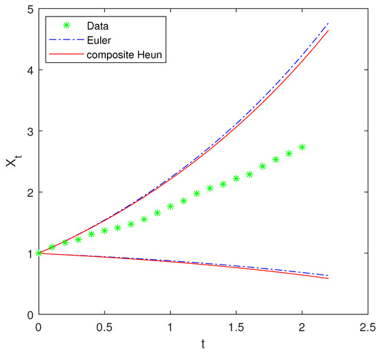
Figure 1. Sample data and $\alpha$-paths of $X_t$ in Example 5.

Example 6. 

Assume an uncertain process $X_t$ satisfies an uncertain delay differential equation

$$\left\{\begin{array}{c}d{X}_t=({\mu }_1{X}_t+{\mu }_2{X}_{t-0.2})dt+({\mu }_3{X}_t+{\mu }_4{X}_{t-0.2})d{C}_t,t\in [0,3.2],\hfill \\ X_t=1,t\in [-0.2,0],\hfill \end{array}\right.$$

(20)

with four unknown parameters ${\mu }_1,{\mu }_2,{\mu }_3$ and ${\mu }_4$ to be estimated.

The true parameters in Equation (20) are designated as ${\mu }_1=-3,{\mu }_2=2,{\mu }_3=1$ and ${\mu }_4=-0.4.$ There are 16 groups of observations generated, which are shown in Table 3. Using the system of Equation (5), the estimations ${\mu }_1$, ${\mu }_2$, ${\mu }_3$ and ${\mu }_4$ are the solutions of the following equations

$$\left\{\begin{array}{c}\hfill {\displaystyle \frac{1}{16}}{\displaystyle \sum _{n=0}^{15}}\left({\displaystyle \frac{x_{t_{n+1}}-x_{t_n}}{({\mu }_3{x}_{t_n}+{\mu }_4{x}_{t_{n-1}})h}}-{\displaystyle \frac{(1-\theta )({\mu }_1{x}_{t_n}+{\mu }_2{x}_{t_{n-1}})}{{\mu }_3{x}_{t_n}+{\mu }_4{x}_{t_{n-1}}}}-{\displaystyle \frac{\theta \left({\mu }_1\left(x_{t_n}+h({\mu }_1{x}_{t_n}+{\mu }_2{x}_{t_{n-1}})\right)+{\mu }_2{x}_{t_n}\right)}{{\mu }_3{x}_{t_n}+{\mu }_4{x}_{t_{n-1}}}}\right)=0,\\ \hfill {\displaystyle \frac{1}{16}}{\displaystyle \sum _{n=0}^{15}}{\left({\displaystyle \frac{x_{t_{n+1}}-x_{t_n}}{({\mu }_3{x}_{t_n}+{\mu }_4{x}_{t_{n-1}})h}}-{\displaystyle \frac{(1-\theta )({\mu }_1{x}_{t_n}+{\mu }_2{x}_{t_{n-1}})}{{\mu }_3{x}_{t_n}+{\mu }_4{x}_{t_{n-1}}}}-{\displaystyle \frac{\theta \left({\mu }_1\left(x_{t_n}+h({\mu }_1{x}_{t_n}+{\mu }_2{x}_{t_{n-1}})\right)+{\mu }_2{x}_{t_n}\right)}{{\mu }_3{x}_{t_n}+{\mu }_4{x}_{t_{n-1}}}}\right)}^2=1,\\ \hfill {\displaystyle \frac{1}{16}}{\displaystyle \sum _{n=0}^{15}}{\left({\displaystyle \frac{x_{t_{n+1}}-x_{t_n}}{({\mu }_3{x}_{t_n}+{\mu }_4{x}_{t_{n-1}})h}}-{\displaystyle \frac{(1-\theta )({\mu }_1{x}_{t_n}+{\mu }_2{x}_{t_{n-1}})}{{\mu }_3{x}_{t_n}+{\mu }_4{x}_{t_{n-1}}}}-{\displaystyle \frac{\theta \left({\mu }_1\left(x_{t_n}+h({\mu }_1{x}_{t_n}+{\mu }_2{x}_{t_{n-1}})\right)+{\mu }_2{x}_{t_n}\right)}{{\mu }_3{x}_{t_n}+{\mu }_4{x}_{t_{n-1}}}}\right)}^3=0,\\ \hfill {\displaystyle \frac{1}{16}}{\displaystyle \sum _{n=0}^{15}}{\left({\displaystyle \frac{x_{t_{n+1}}-x_{t_n}}{({\mu }_3{x}_{t_n}+{\mu }_4{x}_{t_{n-1}})h}}-{\displaystyle \frac{(1-\theta )({\mu }_1{x}_{t_n}+{\mu }_2{x}_{t_{n-1}})}{{\mu }_3{x}_{t_n}+{\mu }_4{x}_{t_{n-1}}}}-{\displaystyle \frac{\theta \left({\mu }_1\left(x_{t_n}+h({\mu }_1{x}_{t_n}+{\mu }_2{x}_{t_{n-1}})\right)+{\mu }_2{x}_{t_n}\right)}{{\mu }_3{x}_{t_n}+{\mu }_4{x}_{t_{n-1}}}}\right)}^4={\displaystyle \frac{21}{5}}.\end{array}\right.$$

(21)

Table 3. Sample data in Example 6.

n	0	1	2	3	4	5	6	7	8	9	10	11	12	13	14	15	16
$t_n$	0	0.2	0.4	0.6	0.8	1.0	1.2	1.4	1.6	1.8	2.0	2.2	2.4	2.6	2.8	3.0	3.2
$x_{t_n}$	1	0.9000	0.5691	0.6277	0.4261	0.4432	0.2630	0.2909	0.1911	0.2357	0.1719	0.1644	0.1241	0.1122	0.0949	0.0832	0.0706

Taking $\theta =0.5$, it is easy to calculate that Equation (21) has an estimation

$$({\widehat{\mu }}_1,{\widehat{\mu }}_2,{\widehat{\mu }}_3,{\widehat{\mu }}_4)=(-2.8164,1.9076,0.7880,-0.0674).$$

Therefore, the estimated equation is

$$\left\{\begin{array}{c}d{X}_t=(-2.8164X_t+1.9076X_{t-0.2})dt+(0.7880X_t-0.0674X_{t-0.2})d{C}_t,t\in [0,3.2],\hfill \\ X_t=1,t\in [-1,0].\hfill \end{array}\right.$$

Solving the system of Equation (21) via the Euler scheme, we get the estimated equation

$$\left\{\begin{array}{c}d{X}_t=(-3.5973X_t+2.4569X_{t-0.2})dt+(0.4862X_t-0.0339X_{t-0.2})d{C}_t,t\in [0,3.2],\hfill \\ X_t=1,t\in [-1,0].\hfill \end{array}\right.$$

Table 4 demonstrates that the method of moments via the composite Heun scheme outperforms the Euler scheme. According to Figure 2, the whole observed data of $X_t$ lie in the region between the $0.01$-path and the $0.90$-path, which indicates that both estimation methods are acceptable.

Table 4. The biases of Example 6.

	$|{\mathit{\mu }}_1-{\widehat{\mathit{\mu }}}_1|$	$|{\mathit{\mu }}_2-{\widehat{\mathit{\mu }}}_2|$	$|{\mathit{\mu }}_3-{\widehat{\mathit{\mu }}}_3|$	$|{\mathit{\mu }}_4-{\widehat{\mathit{\mu }}}_4|$
Euler	0.5973	0.4569	0.5138	0.3661
Composite Heun	0.1836	0.0924	0.2120	0.3326

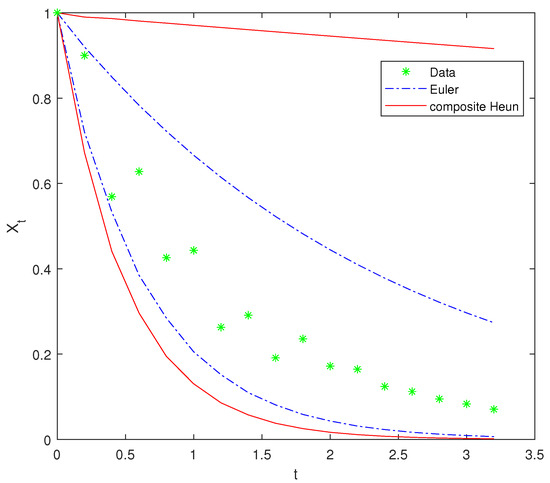
Figure 2. Sample data and $\alpha$-paths of $X_t$ in Example 6.

Example 7. 

Consider the following uncertain delay differential equation

$$\left\{\begin{array}{c}d{X}_t=({\mu }_1+{\mu }_2{X}_{t-0.2})dt+{\mu }_{3}d{C}_t,t\in [0,4.8],\hfill \\ X_t=0.5t+1,t\in [-0.3,0],\hfill \end{array}\right.$$

(22)

with three parameters ${\mu }_1,$ ${\mu }_2,$ and ${\mu }_3$ to be estimated.

The true parameters in Equation (22) are designated as ${\mu }_1=0.4,$ ${\mu }_2=0.1,$ and ${\mu }_3=0.8.$ There are 16 groups of observations generated, which are shown in Table 5. According to Equation (13), the estimations of ${\mu }_1,$ ${\mu }_2,$ and ${\mu }_3$ are the solutions of the following equations

$$\left\{\begin{array}{c}{\displaystyle \frac{1}{16}}{\displaystyle \sum _{n=0}^{15}}{\displaystyle \frac{x_{t_{n+1}}-x_{t_n}-h\left({\mu }_1+\left((1-\theta ){\overline{x}}_{t_{n-1}}+\theta {\overline{x}}_{t_n}\right){\mu }_2\right)}{{\mu }_{3}h}}=0,\hfill \\ {\displaystyle \frac{1}{16}}{\displaystyle \sum _{n=0}^{15}}{\left({\displaystyle \frac{x_{t_{n+1}}-x_{t_n}-h\left({\mu }_1+\left((1-\theta ){\overline{x}}_{t_{n-1}}+\theta {\overline{x}}_{t_n}\right){\mu }_2\right)}{{\mu }_{3}h}}\right)}^2=1,\hfill \\ {\displaystyle \frac{1}{16}}{\displaystyle \sum _{n=0}^{15}}{\left({\displaystyle \frac{x_{t_{n+1}}-x_{t_n}-h\left({\mu }_1+\left((1-\theta ){\overline{x}}_{t_{n-1}}+\theta {\overline{x}}_{t_n}\right){\mu }_2\right)}{{\mu }_{3}h}}\right)}^3=0,\hfill \end{array}\right.$$

(23)

where

$$\begin{array}{c}\hfill {\overline{x}}_{t_{n-1}}={\displaystyle \frac{1}{3}}{x}_{t_n}+{\displaystyle \frac{2}{3}}{x}_{t_{n-1}},{\overline{x}}_{t_n}={\displaystyle \frac{1}{3}}{x}_{t_{n+1}}+{\displaystyle \frac{2}{3}}{x}_{t_n},\end{array}$$

which are obtained by linear interpolation. The observations of ${\overline{X}}_{t_n}$ are also shown in Table 5. Taking $\theta =0.4$, it is easy to calculate that Equation (23) yields an estimation

$$({\widehat{\mu }}_1,{\widehat{\mu }}_2,{\widehat{\mu }}_3)=(0.3594,0.1096,0.8599).$$

Therefore, the estimated equation is

$$\left\{\begin{array}{c}d{X}_t=(0.3594+0.1096X_{t-0.2})dt+0.8599d{C}_t,t\in [0,4.8],\hfill \\ X_t=0.5t+1,t\in [-1,0].\hfill \end{array}\right.$$

Solving the system of Equation (23) via the Euler scheme, we get the estimated equation

$$\left\{\begin{array}{c}d{X}_t=(0.3379+0.1267X_{t-0.2})dt+0.8600d{C}_t,t\in [0,4.8],\hfill \\ X_t=0.5t+1,t\in [-1,0].\hfill \end{array}\right.$$

Table 5. Sample data in Example 7.

n	0	1	2	3	4	5	6	7	8	9	10	11	12	13	14	15	16
$t_n$	0	0.3	0.6	0.9	1.2	1.5	1.8	2.1	2.4	2.7	3.0	3.3	3.6	3.9	4.2	4.5	4.8
$x_{t_n}$	1	1.1000	1.0647	1.1133	1.2314	1.2574	1.2577	1.5619	1.5889	1.8360	1.9894	2.2635	2.9276	3.1762	2.7324	3.4564	4.0529
${\overline{x}}_{t_n}$	1.0333	1.0882	1.0809	1.1527	1.2401	1.2575	1.3591	1.5702	1.6699	1.8871	2.0808	2.4849	3.0105	3.0283	2.9737	3.6552

Table 6 reveals that the performance of the method of moments via the composite Heun scheme is superior to the Euler scheme. As shown in Figure 3, the total observed data of $X_t$ fall in the region between the $0.25$-path and the $0.90$-path, which shows the two estimation methods are acceptable.

Table 6. The biases of Example 7.

	$|{\mathit{\mu }}_1-{\widehat{\mathit{\mu }}}_1|$	$|{\mathit{\mu }}_2-{\widehat{\mathit{\mu }}}_2|$	$|{\mathit{\mu }}_3-{\widehat{\mathit{\mu }}}_3|$
Euler	0.0621	0.0267	0.0600
Composite Heun	0.0406	0.0096	0.0599

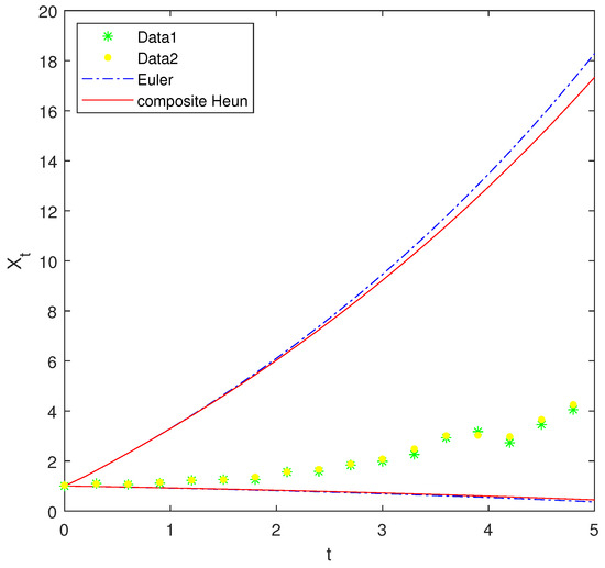
Figure 3. Sample data and $\alpha$-paths of $X_t$ in Example 7.

5. Uncertain Delay Stock Model

Andersen et al. [28] proposed the option pricing formula associated with Black–Scholes diffusion

$$d{S}_t=\mu S_{t}dt+\sigma S_{t}d{W}_t,$$

(24)

where $S_t$ is the option price, $\mu$ and $\sigma$ represent the return on assets and the volatility, respectively, and $W_t$ is a one-dimensional standard Brownian motion. However, the volatility is genuinely erratic in its dependence on time. Taking into account how previous occurrences have affected the system’s present and future states, Arriojas et al. [29] proposed a stochastic delay model for stock price. Mao and Sabanis [30] introduced a delay geometric Brownian motion and systematically studied market models targeted for several important financial derivatives. In this paper, we consider the following stochastic delay stock model proposed in [30]

$$\left\{\begin{array}{c}d{S}_t=\mu S_{t}dt+\sigma S_{t-\tau }d{W}_t,0⩽t⩽T,\hfill \\ S_t=\phi \left(t\right),-\tau ⩽t⩽0,\hfill \end{array}\right.$$

(25)

where $\phi \left(t\right)$ is a given function. However, Liu [9] explained that it is not appropriate to use stochastic differential equations to describe stock price, because the variance of its “noise” term $d{W}_t/dt$ tends to $\infty .$ As a counterpart, he made the case that a tool for modeling stock price may be the uncertain differential equation, because the variance of its “noise” term $d{C}_t/dt$ is 1, not $\infty .$ Therefore, $d{C}_t/dt$ can be used to show the noise terms, so we get the following uncertain delay stock model

$$\left\{\begin{array}{c}d{S}_t=\mu S_{t}dt+\sigma S_{t-\tau }d{C}_t,0⩽t⩽T,\hfill \\ S_t=\phi \left(t\right),-\tau ⩽t⩽0.\hfill \end{array}\right.$$

(26)

We consider the closing price for MF stock from 6 May to 2 August 2022 with 62 total trading days, which are illustrated in Table 7. Assume that the closing price of MF stock follows the following uncertain delay stock model

$$\left\{\begin{array}{c}d{S}_t=\mu S_{t}dt+\sigma S_{t-1}d{C}_t,0⩽t⩽31,\hfill \\ S_t=14.77,-1⩽t⩽0.\hfill \end{array}\right.$$

(27)

Table 7. Stock closing price of MF from 6 May to 2 August 2022.

14.48	14.65	14.76	14.67	14.62	14.80	14.86	14.70	14.71
14.80	14.95	14.92	14.52	14.78	14.99	15.00	15.25	15.41
15.53	15.39	15.34	15.22	15.22	15.12	15.21	15.04	15.10
15.15	15.05	14.99	15.18	15.14	14.89	15.10	15.33	15.55
15.98	15.76	16.37	15.71	15.61	15.57	15.36	15.46	15.44
15.24	15.18	15.36	15.26	15.12	15.28	15.36	15.53	15.44
15.55	15.41	15.42	15.33	15.23	15.07	15.28	14.91

These observations of $S_t$ are set as $s_{t_0},s_{t_1},\dots ,s_{t_{61}}.$ Then 32 data points from 6 May to 21 June are used to establish the model, and 30 data points from 22 June to 2 August are employed to make a forecast to test the validity. According to Equation (4), we have

$$\begin{array}{c}\hfill l_n(\mu ,\sigma )={\displaystyle \frac{s_{t_{n+1}}-s_{t_n}-h\mu (1+h\mu \theta )s_{t_n}}{\sigma s_{t_{n-1}}h}}.\end{array}$$

It follows from Equation (5) that we obtain

$$\left\{\begin{array}{c}{\displaystyle \frac{1}{31}}{\displaystyle \sum _{n=0}^{30}}{\displaystyle \frac{s_{t_{n+1}}-s_{t_n}-h\mu (1+h\mu \theta )s_{t_n}}{\sigma s_{t_{n-1}}h}}=0,\hfill \\ {\displaystyle \frac{1}{31}}{\displaystyle \sum _{n=0}^{30}}{\left({\displaystyle \frac{s_{t_{n+1}}-s_{t_n}-h\mu (1+h\mu \theta )s_{t_n}}{\sigma s_{t_{n-1}}h}}\right)}^2=1.\hfill \end{array}\right.$$

(28)

Taking $\theta =0.8$ and using MATLAB (MATLAB R2023a, 23.2.0.2358603, maci64, Optimization Toolbox, “fsolve” function), we can obtain

$$(\widehat{\mu },\widehat{\sigma })=(0.0015,-0.0097).$$

Therefore, the uncertain delay stock model for MF stock is

$$\left\{\begin{array}{c}d{S}_t=0.0015S_{t}dt-0.0097S_{t-1}d{C}_t,0⩽t⩽31,\hfill \\ S_t=14.77,-1⩽t⩽0.\hfill \end{array}\right.$$

(29)

From Figure 4, all observed values lie in the area between the 0.10-path ${\displaystyle S_t^{0.10}}$ and the 0.90-path ${\displaystyle S_t^{0.90}}$, which indicates the estimation $(0.0015,-0.0097)$ is reasonable.

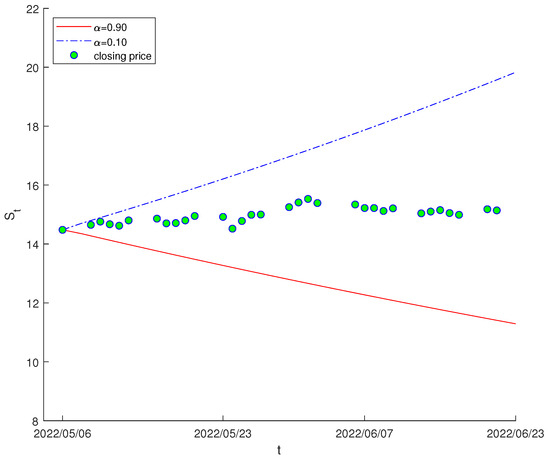
Figure 4. Stock closing price of MF from 6 May to 21 June 2022 and $\alpha$-paths of $S_t$.

To verify the validity of the composite Heun scheme, an algorithm is designed to compute the expected value $E\left[S_t\right]$, which is regarded as the predicted value. From Yao and Chen [31], the inverse uncertainty distribution of $S_t$ is its $\alpha$-path ${\displaystyle S_t^{\alpha }}$, which satisfies the following ordinary differential equation

$$\left\{\begin{array}{c}d{\displaystyle S_t^{\alpha }}=\mu {\displaystyle S_t^{\alpha }}dt+\left|\sigma {\displaystyle S_{t-1}^{\alpha }}\right|{\mathsf{\Phi }}^{-1}\left(\alpha \right)dt,\hfill \\ {\displaystyle S_0^{\alpha }}=S_0.\hfill \end{array}\right.$$

Based on the $\alpha$-path, we have the expected value of $S_t$

$$E\left[S_t\right]={\displaystyle {\int }_0^1}{\displaystyle S_t^{\alpha }}d\alpha .$$

Then the following procedure is provided for obtaining the expected value $E\left[S_t\right].$

• Step 1. Suppose $\alpha =0$ and determine a time t.
• Step 2. Set $\alpha$←$\alpha +0.01$.
• Step 3. Compute ${\displaystyle S_1^{\alpha }},{\displaystyle S_2^{\alpha }},\dots ,{\displaystyle S_T^{\alpha }}$ from the following equation

  $$\left\{\begin{array}{c}d{\displaystyle S_t^{\alpha }}=\mu {\displaystyle S_t^{\alpha }}dt+\left|\sigma {\displaystyle S_{t-1}^{\alpha }}\right|{\mathsf{\Phi }}^{-1}\left(\alpha \right)dt,t\in (0,T],\hfill \\ {\displaystyle S_0^{\alpha }}=S_0,\hfill \end{array}\right.$$

  with numerical method.
• Step 4. Repeat Step 2 and Step 3 99 times, and we can get the ${\displaystyle S_t^{\alpha }}$ for every $\alpha$ as shown in the following Table 8.
  Table 8. Numerical results of ${\displaystyle S_t^{\alpha }}$ with different $\alpha$.

  $\mathit{\alpha }$	0.01	0.02	…	0.99
  ${\displaystyle S_t^{\alpha }}$	${\displaystyle S_t^{0.01}}$	${\displaystyle S_t^{0.02}}$	…	${\displaystyle S_t^{0.99}}$

Table 8 offers the approximation of the inverse uncertainty distribution of $S_t.$

• Step 5 The expected value is

  $$E\left[S_t\right]\approx {\displaystyle \frac{1}{99}}{\displaystyle \sum _{n=1}^{99}}{\displaystyle S_t^{{\displaystyle \frac{n}{100}}}}.$$

We assume that the initial stock price $S_0$ = 15.14, which is the stock price on 21 June and the time $T=30$. By using the above procedure, the stock prices from 22 June to 2 August have the approximation of the expected value $E\left[S_t\right]$, which are shown in Table 9. Figure 5 presents a graphical illustration of the difference between the forecast price and real closing price. From the graph, the performance of the established model by the composite Heun scheme is satisfactory. The root mean square error and the mean absolute error of the predicted values are 0.3707 and 0.4979, respectively.

Table 9. The predicted value against actual value of MF stock price.

Date	Actual Value	Predicted Value
22 June 2022	14.89	15.1627
23 June 2022	15.10	15.1855
24 June 2022	15.33	15.2095
27 June 2022	15.55	15.2348
28 June 2022	15.98	15.2614
29 June 2022	15.76	15.2894
30 June 2022	16.37	15.3186
01 July 2022	15.71	15.3492
04 July 2022	15.61	15.3811
05 July 2022	15.57	15.4143
06 July 2022	15.36	15.4488
07 July 2022	15.46	15.4847
08 July 2022	15.44	15.5220
11 July 2022	15.24	15.5606
12 July 2022	15.18	15.6006
13 July 2022	15.36	15.6419
14 July 2022	15.26	15.6847
15 July 2022	15.12	15.7288
18 July 2022	15.28	15.7744
19 July 2022	15.36	15.8214
20 July 2022	15.53	15.8698
21 July 2022	15.44	15.9196
22 July 2022	15.55	15.9710
25 July 2022	15.41	16.0238
26 July 2022	15.42	16.0780
27 July 2022	15.33	16.1338
28 July 2022	15.23	16.1910
29 July 2022	15.07	16.2498
1 August 2022	15.28	16.3102
2 August 2022	14.91	16.3720

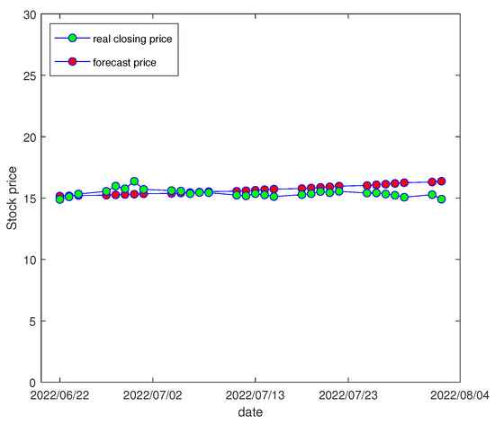
Figure 5. Forecast results of MF stock closing price.

6. Conclusions

In this paper, we introduced a new numerical difference approximation method named the composite Heun scheme for approximating uncertain delay differential equations. The new scheme was successfully applied to estimate parameters in uncertain delay differential equations with both integer and noninteger delays based on the method of moments. The numerical results demonstrated that the composite Heun method achieved higher accuracy than the Euler method. Based on the historical stock price data of Xiamen Airlines, we forecasted the future stock prices and validated the effectiveness of the composite Heun method by comparing actual prices with model-predicted prices. The quantitative results confirmed the efficacy of both the uncertain delay stock model and the composite Heun method.

References

- Bahar, A.; Mao, X. Stochastic delay population dynamics. J. Int. Appl. Math. 2004, 11, 377–400. [Google Scholar]
- Villasana, M.; Radunskaya, A. A delay differential equation model for tumor growth. J. Math. Biol. 2003, 47, 270–294. [Google Scholar] [CrossRef]
- Roussel, M.R. The use of delay differential equations in chemical kinetics. J. Phys. Chem. 1996, 100, 8323–8330. [Google Scholar] [CrossRef]
- Liu, M.; Wang, K.; Hong, Q. Stability of a stochastic logistic model with distributed delay. Math. Comput. Model. 2013, 57, 1112–1121. [Google Scholar] [CrossRef]
- Shen, Y.; Meng, Q.; Shi, P. Maximum principle for mean-field jump–diffusion stochastic delay differential equations and its application to finance. Automatica 2014, 50, 1565–1579. [Google Scholar] [CrossRef]
- Tian, T.; Burrage, K.; Burrage, P.M.; Carletti, M. Stochastic delay differential equations for genetic regulatory networks. J. Comput. Appl. Math. 2007, 205, 696–707. [Google Scholar] [CrossRef]
- Ma, H.; Liu, B. Optimal control problem for risk-sensitive mean-field stochastic delay differential equation with partial information. Asian J. Control 2017, 19, 2097–2115. [Google Scholar] [CrossRef]
- Kahneman, B.D.; Tversky, A. Prospect theory: An analysis of decisions under risk. Econometrica 1979, 47, 263–291. [Google Scholar] [CrossRef]
- Liu, B. Uncertainty Theory, 2nd ed.; Springer: Berlin/Heidelberg, Germany, 2007. [Google Scholar]
- Liu, B. Some research problems in uncertainty theory. J. Uncertain Syst. 2009, 3, 3–10. [Google Scholar]
- Jadlovská, I.; Li, T. A note on the oscillation of third-order delay differential equation. Appl. Math. Lett. 2025, 167, 109555. [Google Scholar] [CrossRef]
- Batiha, B.; Alshammari, N.; Aldosari, F.; Masood, F.; Bazighifan, O. Nonlinear Neutral Delay Differential Equations: Novel Criteria for Oscillation and Asymptotic Behavior. Mathematics 2025, 13, 147. [Google Scholar] [CrossRef]
- Liu, B. Fuzzy process, hybrid process and uncertain process. J. Uncertain Syst. 2008, 2, 3–16. [Google Scholar]
- Barbacioru, C. Uncertainty functional differential equations for finance. Surv. Math. Appl. 2010, 5, 275–284. [Google Scholar]
- Ge, X.; Zhu, Y. Existence and uniqueness theorem for uncertain delay differential equations. J. Comput. Inf. Syst. 2012, 8, 8341–8347. [Google Scholar]
- Wang, X.; Ning, Y. Stability of uncertain delay differential equation. J. Intell. Fuzzy Syst. 2017, 32, 2655–2664. [Google Scholar] [CrossRef]
- Jia, L.; Sheng, Y. Stability in distribution for uncertain delay differential equation. Appl. Math. Comput. 2019, 343, 49–56. [Google Scholar] [CrossRef]
- Yao, K.; Liu, B. Parameter estimation in uncertain differential equations. Fuzzy Optim. Decis. Mak. 2020, 19, 1–12. [Google Scholar] [CrossRef]
- Liu, Z. Generalized moment estimation for uncertain differential equations. Appl. Math. Comput. 2021, 392, 125724. [Google Scholar] [CrossRef]
- Yao, L.; Zhang, G.; Sheng, Y. Generalized moment estimation of multi-dimensional uncertain differential equations. J. Intell. Fuzzy Syst. 2023, 44, 2427–2439. [Google Scholar] [CrossRef]
- Sheng, Y.; Yao, K.; Chen, X. Least squares estimation in uncertain differential equations. IEEE. Trans. Fuzzy Syst. 2019, 28, 2651–2655. [Google Scholar] [CrossRef]
- Liu, Z.; Jia, L. Moment estimations for parameters in uncertain delay differential equations. J. Intell. Fuzzy Syst. 2020, 39, 841–849. [Google Scholar] [CrossRef]
- Gao, Y.; Gao, J.; Yang, X. Parameter estimation in uncertain delay differential equations via the method of moments. Appl. Math. Comput. 2022, 431, 127311. [Google Scholar] [CrossRef]
- Li, A.; Xia, Y. Parameter estimation of uncertain differential equations with estimating functions. Soft Comput. 2024, 28, 77–86. [Google Scholar] [CrossRef]
- He, L.; Zhu, Y.; Gu, Y. Nonparametric estimation for uncertain differential equations. Fuzzy Optim. Decis. Mak. 2023, 22, 697–715. [Google Scholar] [CrossRef]
- He, L.; Zhu, Y. Nonparametric estimation for uncertain fractional differential equations. Chaos Solitons Fractals 2024, 178, 114342. [Google Scholar] [CrossRef]
- Zhou, S.; Tan, X.; Wang, X. Moment estimation based on the composite Heun scheme for parameters in uncertain differential equations. J. Intell. Fuzzy Syst. 2023, 45, 4239–4248. [Google Scholar] [CrossRef]
- Andersen, T.G.; Benzoni, L.; Lund, J. An empirical investigation of continuous-time equity return models. J. Financ. 2002, 57, 1239–1284. [Google Scholar] [CrossRef]
- Arriojas, M.; Hu, Y.; Mohammed, S.E.; Pap, G. A delayed Black and Scholes formula. Stoch. Anal. Appl. 2007, 25, 471–492. [Google Scholar] [CrossRef]
- Mao, X.; Sabanis, S. Delay geometric Brownian motion in financial option valuation. Stochastics Int. J. Probab. Stoch. Processes 2013, 85, 295–320. [Google Scholar] [CrossRef][Green Version]
- Yao, K.; Chen, X. A numerical method for solving uncertain differential equations. J. Intell. Fuzzy Syst. 2013, 25, 825–832. [Google Scholar] [CrossRef]
Disclaimer/Publisher’s Note: The statements, opinions and data contained in all publications are solely those of the individual author(s) and contributor(s) and not of MDPI and/or the editor(s). MDPI and/or the editor(s) disclaim responsibility for any injury to people or property resulting from any ideas, methods, instructions or products referred to in the content. |
© 2025 by the authors. Licensee MDPI, Basel, Switzerland. This article is an open access article distributed under the terms and conditions of the Creative Commons Attribution (CC BY) license (https://creativecommons.org/licenses/by/4.0/).