Abstract
We develop and analyze a reaction-diffusion model describing the early spatial dynamics of viral infection in tissue, incorporating key components of the innate immune system: inflammatory cytokines and circulating macrophages. The system couples three spatial partial differential equations (for uninfected cells, infected cells, and virus particles) with two ordinary differential equations (for cytokines and activated macrophages), and it includes time delays related to intracellular viral replication. In the absence of macrophage degradation, we derive analytical expressions for the total viral load and the wave speed, and we identify explicit immune control thresholds in terms of the virus replication number and the strength of the immune response. In the presence of macrophage degradation, simulations reveal that increasing macrophage turnover accelerates wave propagation and increases viral burden. These results highlight the critical role of innate immune feedback, modulated by effector degradation, in shaping the spatial outcome of infection. Depending on the values of viral replication number and the strength of the immune response, infection can be immediately suppressed, or it can propagate with gradual extinction due to the time-dependent immune response, or it can persistently propagate in the tissue in the form of a reaction-diffusion wave.
Keywords:
infection propagation; innate immunity; cytokine signaling; macrophage activation; reaction-diffusion system MSC:
35K57; 92C32
1. Introduction
Viral infections remain a major global health concern due to their rapid transmissibility and potential to cause significant morbidity and mortality. Epidemics such as seasonal influenza and pandemics like COVID-19 have underscored the urgency of understanding the biological mechanisms underlying virus–host interactions, particularly during the early stages of infection [1,2]. Once inside host tissue, viruses infect susceptible cells, hijack their replication machinery, and produce progeny virions. These viral particles propagate through local diffusion and direct intercellular transmission, forming spatial infection waves [2,3].
The immune system responds with a layered defense strategy involving both innate and adaptive responses. The innate immune system acts rapidly, within hours, and provides a generalized defense before the adaptive immune system becomes fully engaged. Central to this early response are inflammatory cytokines and immune cells such as macrophages, which shape the tissue environment and limit viral replication [4,5]. Upon detecting viral components, infected cells initiate signaling cascades leading to the production of cytokines such as tumor necrosis factor (TNF), interleukin-6 (IL-6), and interferons. These molecules orchestrate immune responses and trigger programmed cell death (PCD) in infected cells, thereby halting viral replication [6]. Several forms of PCD have been implicated in viral infections, including apoptosis, pyroptosis, necroptosis, and PANoptosis—a combined form integrating features of all three. Although essential, dysregulated or excessive cell death may result in tissue damage and systemic inflammation [5,7]. In our model, inflammatory cytokines are secreted by both infected cells and activated macrophages, enhancing immune-mediated destruction of infected cells and establishing a feedback loop that can contain infection, depending on parameter values.
Macrophages are key innate immune effectors involved in pathogen detection, phagocytosis, cytokine production, and immune regulation. During infection, blood monocytes are recruited to the tissue and differentiate into macrophages, which can polarize into M1 (pro-inflammatory, microbicidal) or M2 (anti-inflammatory, tissue-repairing) states depending on environmental signals [4,8]. Here, we focus on circulating macrophages that become activated through interactions with virus particles and pro-inflammatory cytokines. Once activated, they amplify the cytokine pool and facilitate the clearance of infected cells, while their population dynamics are shaped by production, activation, and degradation processes.
The spatial spread of infection arises from the interaction between viral replication, diffusion, and immune activity. Reaction–diffusion models provide a powerful framework to study such phenomena, enabling the analysis of wavefront propagation and spatiotemporal dynamics [3,9,10,11]. The wave speed reflects the efficiency of viral expansion, while the total viral load (integrated spatial virus concentration) quantifies infection burden [10]. Building on this framework, we extend classical models by integrating immune regulation through cytokine signaling and macrophage activation [12,13]. Our system consists of five key components: uninfected cells (U), infected cells (F), virus particles (V), inflammatory cytokines (S), and activated macrophages (N). Virus and infected cells are modeled as spatially distributed quantities, while S and N are treated as spatially homogeneous due to their redistribution by blood circulation [9,14].
The novelty of this study lies in the formulation and analysis of a hybrid model that combines virus diffusion with nonlinear immune feedback mediated by cytokines and macrophages. We incorporate a biologically motivated time delay representing intracellular viral replication and couple it with immune-mediated cell death. We also model macrophage activation by virus and cytokines, which further contributes to immune regulation. Analyzing the system, we derive conditions for infection spreading, compute the traveling wave speed and viral load, and complement the theoretical results with numerical simulations. These simulations reveal how macrophage degradation rates and cytokine feedback strength critically affect infection dynamics. Altogether, this study provides new insights into the thresholds that separate controlled from uncontrolled viral propagation.
The remainder of this paper is structured as follows. Section 2 presents the mathematical formulation of the model. Section 3 analyzes the traveling wave solutions and conditions for their existence. Section 4 provides numerical simulations and investigates the impact of immune parameters. Section 5 discusses biological implications and outlines future research directions.
Figure 1 provides a schematic representation of the main biological interactions considered in this study. Virus particles infect susceptible cells and induce their death through cytokine-mediated signaling. Infected cells and activated macrophages both secrete inflammatory cytokines, which amplify immune-mediated clearance of infected cells. Viral particles also stimulate the activation of circulating macrophages, represented in the diagram by the transition from inactive macrophages M to activated macrophages N. In the mathematical model developed below, we do not introduce a separate variable M; instead, the pool of inactive macrophages is treated implicitly, so that the total number of circulating macrophages is kept constant. This modeling assumption reflects the idea that, during the early stages of infection considered here, macrophage activation occurs on a faster timescale than systemic recruitment and therefore dominates the dynamics.
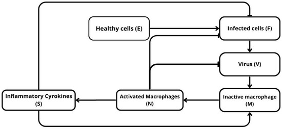
Figure 1.
Schematic representation of the model. Healthy cells U are infected by the virus V and become infected cells F, which produce more virus and stimulate the immune response. The virus activates circulating macrophages M into activated macrophages N, which in turn release inflammatory cytokines S. These cytokines amplify macrophage activation and promote the elimination of infected cells.
2. Reaction-Diffusion Model of Viral Infection
2.1. Model Formulation
The propagation of viral infection in an infected tissue occurs at the first stage of the innate immune response. The replication of the virus within infected cells promotes the production of inflammatory cytokines by both infected cells and circulating macrophages. Inflammatory cytokines, in turn, trigger the programmed cell death of infected cells. We consider the following system of equations:
where ,
Here, represents the concentration of uninfected target cells, such as epithelial cells, while denotes the concentration of infected cells, and corresponds to activated circulating macrophages. The virus concentration is represented by and the inflammatory cytokines concentration is denoted by Unlike and which depend on both time and space, the variables S and N depend only on time due to their fast distribution within the tissue via blood circulation and diffusion.
The right-hand side of Equation (1) represents the rate of infection of uninfected cells by virus. A similar term enters the next equation with sign plus. The other terms in the right-hand side of this equation describe the rate of infected cell death due to inflammatory cytokines, their elimination by activated macrophages, and their death independent of the immune response. Equation (3) for the virus concentration in the infected tissue describes, respectively, its diffusion, production by the infected cells, its elimination by macrophages, and its death independent of the immune response [15]. The rate of macrophage activation by virus antigens and by inflammatory cytokines is given in the right-hand side of Equation (4). The activation rate is limited by the total level of circulating macrophages . The last term in this equation represents deactivation or death of macrophages. Note that the level of virus antigens in the body, which determines the activation of macrophages, is proportional to the total virus concentration in the tissue. The last equation for inflammatory cytokines includes the rate of their production by infected cells proportional to their total quantity in the tissue, their consumption in the interaction with infected cells, production by activated macrophages, and their degradation.
2.2. Infection Spreading as a Wave
We are looking for a solution of system (1)–(5) in the form of a traveling wave: and where and c is the wave speed. Since the two last equations of the system do not depend on the space variable, We obtain the following:
where and We consider the following limits at infinity:
where is the initial concentration of the uninfected cells, and is their unknown final concentration. Along with this final concentration, we will determine the integral of the viral load and the wave speed c.
3. System Without Degradation of Activated Macrophages
We begin the study of System (6)–(10) with the case . This assumption simplifies the analysis and will allow us to determine from a single algebraic equation. Under this assumption, we have . Therefore, we consider the following system:
Integrating (12), we obtain:
Integration of the difference of Equations (12) and (13) gives:
From Equation (14), we express as follows:
Thus, we obtain the following system of equations with respect to the variables (), , and :
From (17) and (19), we obtain the following equation:
Substituting this expression into (18), we derive the equation with respect to :
where
3.1. Existence of Solution
We will now study the existence of solutions of Equation (20) for .
Proposition 1.
Proof.
Write Equation (20) in the form
with . Define and .
First, note that since . Moreover, as , we have , and because as , one has . Hence, while (finite). Thus, for sufficiently small , we have .
Differentiate both sides on :
so at ,
Since , we obtain . Therefore, if then . Consequently, there exists such that for all we have . Combined with as and continuity of on , the Intermediate Value Theorem yields some with . This proves the claim. □
Define and compute
with
Proposition 2.
If
then
If
then there is such that
Proof.
The sign of the second derivative of for coincides with the sign of the difference for , or with the sign of the polynomial
Note that . Therefore,
Theorem 1.
If condition (22) is satisfied, then Equation (20) has a solution if and only if inequality (21) holds. Moreover, this solution is unique. If condition (24) is satisfied, then there exists such that Equation (20) has a solution if and only if . This solution is unique for , and there are two solutions for .
Proof.
Let (22) be satisfied. According to Proposition 2, the function is concave for . Since Equation (20), that is,
has solution , then it has a unique solution if , and no such solution otherwise.
Now, let (24) be satisfied. Then existence of a solution for follows from Proposition 1. Suppose that the solution is not unique and, for certainty, there are two solutions, , . The derivatives of the left-hand side and of the right-hand side of Equation (20) are equal to each other between solutions and and between solutions and . Therefore, at least for two values of . According to Proposition 2, is a positive function in the interval with a single minimum. Since , then the equation can have at most one solution. This contradiction proves the uniqueness of the solution of Equation (20) in .
Similar arguments show that Equation (20) does not have solution in for R sufficiently small; in particular, if . Hence, there is such that Equation (20) does not have solutions for .
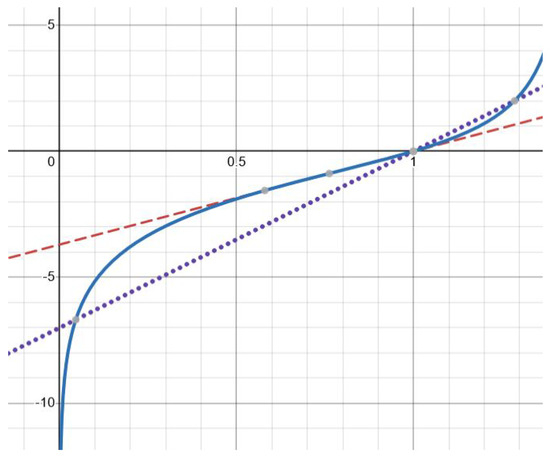
Finally, there are exactly two solutions for (Figure 2). This follows from a similar analysis of the derivatives and . The details are left to the reader. The theorem is proved. □
Figure 2.
Graphical solution of Equation (20) with function (solid line) and , where (dotted line) and (dashed line). There is one solution for the former and two solutions for the latter. The values of the parameters are as follows: , (dashed line), (dotted line).
Approximate Solution
Analysis of Equation (20) shows that its solution converges to 0 as R increases. Therefore, for R sufficiently large, , and can be neglected in the left-hand side of this equation. On the other hand, . Hence, we obtain the approximate equality . Thus, we can find
Note that and depend on the wave speed c. We will determine it in the next section.
3.2. Wave Speed
In order to determine the wave speed, we use the linearization method. We replace u by at Therefore, we obtain the following linearized system of equations for f and v:
The integral is considered here as a given constant. Let us look for the solution of this system in the form Substituting these functions into Equations (26) and (27), we obtain the following:
In order to find the minimal wave speed, we should determine the minimal value of c for which this system of equations has a positive solution since the solution is decreasing at infinity. Introducing an independent parameter and excluding from the previous two equations, we obtain the following equation:
where
Hence,
where
Here
and is the value for which the denominator vanishes. Such value exists if
If condition (31) is not satisfied, then the function is defined for all , and . The minimal wave speed in this case equals zero.
Note that this condition is not explicit. Indeed, the integral depends on the unknown wave speed. Therefore, P and the function also depend on it, and (30) is an equation with respect to c. However, P can be estimated by the respective values for and :
If
then . If inequality (32) is opposite, then is larger than . We will use these values below to determine different regimes of infection progression.
3.3. Regimes of Infection Progression
We derived above two critical conditions that determine infection progression. Condition (21) provides the existence of solution of Equation (20) in the interval . Condition (31) implies that the wave speed is positive. Both of them are necessary conditions of the existence of the infection wave, but their sufficiency is not proved.
Note that such that Condition (21) coincides with Condition (31) if . Hence, if
then neither Condition (21) nor (31) is satisfied, and the infection wave does not exist.
However, infection can spread in a transient regime with gradual extinction. In order to illustrate this regime, let us consider System (1)–(5) under the assumption that . This means that the concentrations of inflammatory cytokines and macrophages remain zero (as for the initial condition). Hence, this model is the same as in the case of infection spreading in cell culture [16]. It propagates if (cf. [17]). Note that is obtained from the virus replication number R if .
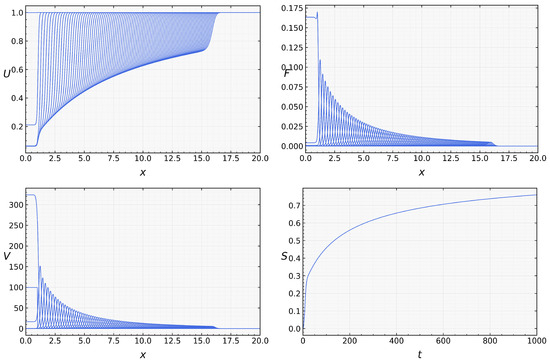
We now return to the full system with assuming that . In the beginning of the simulations, when the concentration of macrophages is low, infection propagates as for the case without macrophages (Figure 3). However, since their concentration grows with time, viral load decreases and converges to zero. Thus, in this example, infection is progressively eliminated by the innate immune response. Numerical simulations of system (1)–(5) were performed to illustrate the spatiotemporal evolution of infection and immune response [18].
On the other hand, if
then both conditions (21) and (31) are satisfied, and we observe propagation of the infection wave. Note that the analytical results obtained above do not prove the existence and stability of such wave, but numerical simulations confirm infection propagation as a reaction-diffusion wave (Figure 4). The analytical and numerical values of the viral load and wave speed are in good agreement. The analytic value of viral load is , and its numerical value is The analytic value of the wave speed is , and the numerical value is .
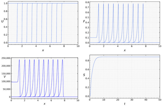
Figure 5 illustrates the dependence of the wave speed c and the viral load on the time delay for the three parameter sets considered. In all cases, both quantities decrease as increases. Comparison of the curves shows that increasing the macrophage clearance rate has little effect on the wave speed c but substantially reduces the viral load (via a reduction in the replication number ), whereas increasing the diffusion coefficient D significantly increases the wave speed and the viral load.
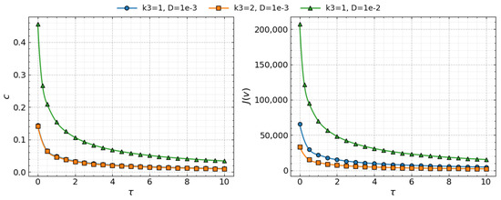
Figure 5.
Left: Comparison of the numerical values (symbols) and analytic values (lines) of the wave speed c as a function of the time delay Right: Comparison of the numerical values (symbols) and analytic values (lines) of the viral load as a function of time delay . Three cases are shown: (circles), (squares), and (triangles). Values of parameters: , , , , , , , , , , cm, (copy/mL), (cell/mL), , , , , .
In order to continue the analysis of the regimes of infection progression, suppose that Condition (32) is satisfied. Then, . We will consider now the case where Condition (21) is satisfied and Condition (31) is not satisfied. This means that
and
For any , so that these two conditions are compatible. The first condition provides infection progression, while the second condition means that the wave speed equals zero; that is, the infection wave extincts. We have previously observed such behavior in [19] for the model with resident macrophages.
4. System with Degradation of Activated Macrophages
We consider System (6)–(10). As in Section 3, we derive the equation for :
where
Note that for , we have , and we reduce this equation to the previous one.
Set
Let us determine the behavior of this function as assuming that . Note that and , since . Therefore, , since . Dividing the numerator and denominator of N by this expression, we conclude that . Hence, . We conclude that
Thus, the right-hand side of Equation (35) converges to as . Therefore, this equation has a solution if
By virtue of approximation in the vicinity of , we conclude that is bounded. Hence, Condition (36) is equivalent to the following condition:
In order to determine , we note that and , since . Therefore,
We reduce this system to a single equation with respect to S:
It has a positive solution if
This solution can be found as a solution of the corresponding quadratic equation.
We proved the following proposition.
Proposition 3.
Set
Since is a decreasing function of as a solution of Equation (38), this is also true for and for . Hence, the critical value of R decreases with increases in the macrophage death rate.
If Equation (35) has a solution , then we can determine viral load and wave speed (cf. Section 3). However, the calculations becomes excessively complex and do not lead to an explicit analytical formula. Hence, we restrict their investigation to numerical simulations (Figure 6). Both viral load and wave speed increase with the increase in and decrease with an increase in . Hence, increasing the macrophage death rate promotes infection propagation, while elimination of infected cells by macrophages downregulates it.
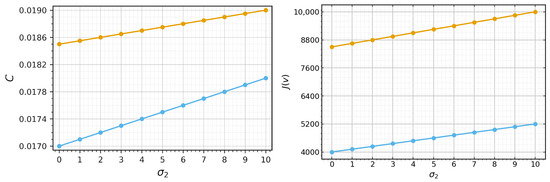
Figure 6.
Left: wave speed c as a function of , where the orange curve represents the case and the blue curve represents the case . Right: viral load as a function of , where the orange curve represents the case and the blue curve represents the case Values of parameters: , ,, , , , , , , , cm, (copy/mL), (cell/mL), , , , , , , .
5. Discussion
In this study, we developed and analyzed a spatial mathematical model that captures the early dynamics of viral infection in tissue, explicitly incorporating key elements of the innate immune response—namely, inflammatory cytokines and circulating macrophages.
The model couples one reaction-diffusion PDE (for the virus) with two reaction PDEs (for uninfected and infected cells), in addition to the ODEs for cytokines and activated macrophages. This structure allows us to explore both local and systemic effects, particularly traveling infection fronts.
The model integrates the most essential features of viral infections and immune response; in particular, infection of healthy cells by viral particles and virus production by infected cells, clearance of infected cells via cytokines and macrophages, cytokine production by infected cells and activated macrophages, activation of macrophages by both cytokines and virus, and optional degradation of activated macrophages (modeled via ).
Together, these interactions form a nonlinear feedback system, where immune activation is dynamically modulated by infection burden. This feedback is biologically supported by experimental studies on cytokine signaling and macrophage polarization [4,20,21,22,23].
An important property of the model is its ability to represent the feedback loop formed by cytokines and activated macrophages. Infected cells trigger cytokine release, which promotes macrophage activation. In turn, these macrophages enhance cytokine production and contribute to the elimination of infected cells [22,23]. This forms a positive feedback loop that may facilitate rapid viral clearance.
However, if the degradation of activated macrophages is included (), the feedback becomes self-limiting. This addition reflects biologically realistic processes such as macrophage exhaustion, apoptosis, or immune regulation [5,21]. The loss of effector cells dampens cytokine production, weakening immune control and allowing broader viral spread.
5.1. Characterization of Infection Progression
In the idealized scenario , activated macrophages persist indefinitely, and the system simplifies. Considering the traveling wave of infection spreading, we derived an explicit nonlinear equation for the fraction of surviving uninfected cells . This equation links to the total viral load and wave speed c. It provides a necessary condition for the infection spreading in the tissue in the form of a traveling wave.
Solvability of this equation provides an important characterization of the progression of viral infection. It is determined by the virus replication number R expressed through the parameters of the model. In the case without macrophages (), or if they do not eliminate infected cells and free virions (), the virus replication number introduced in this work coincides with the virus replication number considered in [16] for infection spreading in cell culture without immune response. As shown in this previous work, viral infection spreads in cell culture if and extincts otherwise. The solvability condition of this equation in the case of immune response provided by circulating macrophages is given by the inequality , where is a positive parameter determined by the coefficients of the model. Hence, the region in the parameter space corresponding to infection progression shrinks due to the immune response, while the region of infection elimination increases (cf. [13,24]).
It should be noted, however, that condition is a sufficient condition for the solvability of this equation but not necessary. It appears that in some parameter range, it can be solvable in a narrow interval . Moreover, there are two solutions of this equation satisfying . We can expect that two waves exist in this case, one stable and the other unstable, and that initial conditions should be sufficiently large to provide convergence to the stable wave versus extinction of the infection and convergence to zero. This conjecture is not yet confirmed by direct numerical simulations since the parameter range of possible bistability is narrow, and the choice of initial conditions should be very precise.
In addition to the solvability of the equation for , we determine the wave speed using the linearization method. The minimal wave speed is positive if , where P is the strength of the immune response. This parameter is expressed through the coefficients of the model and through the viral load. The latter satisfies a transcendental system of the equation (together with the wave speed), and it does not admit a simple analytical expression, but it can be approximated via the method of successive approximation. Note that, depending on the parameters, we can have or .
These three parameters, , and P, determine the regimes of infection progression. If and , then infection spreads as a traveling wave, while if both inequalities are opposite, it extincts. Though analytical results give only the necessary conditions of infection spreading, these conclusions are confirmed by direct numerical simulations.
An interesting question is whether it is possible to have only one of these conditions satisfied. In this case, we can expect that infection starts its progression but gradually extincts, as was previously observed in the model with resident macrophages [8]. In numerical simulations of the actual model, we could not yet find this regime of infection spreading.
One more regime corresponds to transient infection spreading and its gradual extinction. Since initially, there are no activated macrophages (), infection propagates if . However, since the concentration of macrophages grows with time, then the viral load decreases. In the case of , which is possible since , infection is gradually eliminated by the innate immune response (Figure 3).
If , the model becomes more difficult to analyze. We determine the virus replication number and sufficient conditions of solvability of the equation for . We conclude that higher values of facilitate infection progression. This conclusion is confirmed through direct numerical simulations showing that the infection front propagates more rapidly and reaches higher viral burdens.
5.2. Biological Implications and Model Limitations
The results of this work corroborate biological data about the role of macrophages in the development of viral infections. During respiratory viral infections, circulating monocytes are rapidly recruited into the lungs, where they differentiate into macrophages that participate in viral clearance. These macrophages lower viral load through multiple mechanisms: direct phagocytosis of viral particles and infected epithelial cells, production of antiviral mediators such as nitric oxide and type I interferons, and enhancement of adaptive immunity by presenting viral antigens to T lymphocytes. Experimental studies in influenza virus infection demonstrate that depletion of circulating or alveolar macrophages results in higher viral titers and worsened pathology, while their activation promotes faster viral clearance and improved survival [25,26].
These findings emphasize the dual role of macrophage regulation: while necessary to avoid overactivation and tissue damage, excessive degradation may impair viral containment, especially in early infection [5,6]. Our results underscore a fundamental trade-off in immune dynamics: persistent activation of macrophages is beneficial for rapid viral control, but this requires tight regulation to avoid immunopathology. Conversely, premature degradation of effector cells facilitates viral spread. This suggests that therapeutic strategies enhancing macrophage stability—or delaying their exhaustion—could improve immune effectiveness in early infection phases. Excessive immune suppression might unintentionally promote viral persistence.
Immune response to viral infection is a very complex biological processes, and models of immune response encounter necessarily essential simplifications. In this work, we consider only circulating macrophages, as one of the most important actors in the innate immune response. Resident macrophages were considered in [8], and the adaptive immune response was considered in [27]. Bringing together these different parts of the immune response will require further investigations.
6. Conclusions and Future Directions
In summary, we developed and analyzed a spatially explicit model of viral infection coupled with immune regulation through cytokine signaling and macrophage activation. This study established analytical conditions for infection persistence versus extinction, and it identified the dependence of traveling wave speed and viral load on immune parameters. Numerical simulations supported the theoretical results and illustrated the impact of macrophage degradation on infection dynamics.
This work has several limitations. The model considers only circulating macrophages and a single cytokine variable, whereas real immune responses involve resident macrophages, adaptive immunity, and multiple interacting mediators. Furthermore, parameter values were chosen for theoretical exploration rather than being fitted to experimental data.
Future research should address these limitations by integrating additional immune mechanisms, accounting for spatial migration of immune cells, and calibrating model parameters with biological datasets. Another promising direction is the exploration of stochastic formulations, which may capture variability in early infection events. Together, these extensions would provide a more comprehensive picture of the spatiotemporal dynamics of viral infections.
Author Contributions
Methodology, V.V.; Software, M.B. and L.A.M.; Validation, A.M.; Formal analysis, M.B. and L.A.M.; Investigation, M.B., L.A.M., A.M. and V.V.; Writing—original draft, M.B., L.A.M., A.M. and V.V. All authors have read and agreed to the published version of the manuscript.
Funding
The research was funded by the Russian Science Foundation No. 24-11-00073.
Data Availability Statement
The original contributions presented in this study are included in the article. Further inquiries can be directed to the corresponding authors.
Conflicts of Interest
The authors declare no conflicts of interest.
References
- Sender, R.; Bar-On, Y.M.; Gleizer, S.; Bernshtein, B.; Flamholz, A.; Phillips, R.; Milo, R. The total number and mass of SARS-CoV-2 virions. Proc. Natl. Acad. Sci. USA 2021, 118, e2024815118. [Google Scholar] [CrossRef]
- Yin, J.; McCauley, J.W. Modeling virus spread in tissues. Biophys. J. 1992, 61, 1540–1551. [Google Scholar] [CrossRef]
- Ait Mahiout, L.; Bessonov, N.; Kazmierczak, B.; Volpert, V. Infection spreading in cell culture as a reaction-diffusion wave. ESAIM Math. Model. Numer. Anal. 2022, 56, 791–814. [Google Scholar] [CrossRef]
- Ferrer, M.F.; Thomas, P.; López Ortiz, A.O.; Errasti, A.E.; Charo, N.; Romanowski, V.; Gorgojo, J.; Rodriguez, M.E.; Carrera Silva, E.A.; Gómez, R.M. Junin Virus Triggers Macrophage Activation and Modulates Polarization According to Viral Strain Pathogenicity. Front. Immunol. 2019, 10, 2499. [Google Scholar] [CrossRef]
- Jorgensen, I.; Rayamajhi, M.; Miao, E.A. Programmed cell death as a defense against infection. Nat. Rev. Immunol. 2017, 17, 151–164. [Google Scholar] [CrossRef] [PubMed]
- Kuri, P.; Schieber, N.L.; Thuma, F.; Chojnacki, J.; Karreman, M.A.; Schwab, Y. PANoptosis: A new paradigm of inflammatory programmed cell death. Trends Immunol. 2022, 43, 20–34. [Google Scholar] [CrossRef]
- Camell, C.D.; Sander, J.; Spadaro, O.; Lee, A.; Nguyen, K.Y.; Wing, A.; Goldberg, E.L.; Youm, Y.H.; Brown, C.W.; Elsworth, J.; et al. Inflammasome-driven catecholamine catabolism in macrophages blunts lipolysis during ageing. Nature 2017, 550, 119–123. [Google Scholar] [CrossRef]
- Muñoz-Rojas, A.R.; Kelsey, I.; King, K.Y.; Goodridge, H.S. Tissue-resident macrophages: Multifaceted regulators of tissue homeostasis and immunity. Immunity 2021, 54, 1001–1014. [Google Scholar] [CrossRef]
- Bocharov, G.; Meyerhans, A.; Bessonov, N.; Trofimchuk, S.; Volpert, V. Spatiotemporal dynamics of virus infection spreading in tissues. PLoS ONE 2016, 11, e0168576. [Google Scholar] [CrossRef]
- Mozokhina, A.; Ait Mahiout, L.; Volpert, V. Modeling of viral infection with inflammation. Mathematics 2023, 11, 4095. [Google Scholar] [CrossRef]
- Mok, W.; Stylianopoulos, T.; Boucher, Y.; Jain, R.K. Mathematical modeling of herpes simplex virus distribution in solid tumors: Implications for cancer gene therapy. Clin. Cancer Res. 2009, 15, 2352–2360. [Google Scholar] [CrossRef]
- Reyes-Silveyra, J.; Mikler, A.R. Modeling immune response and its effect on infectious disease outbreak dynamics. Theor. Biol. Med. Model. 2016, 13, 10. [Google Scholar] [CrossRef]
- Nowak, M.A.; May, R.M. Virus Dynamics: Mathematical Principles of Immunology and Virology; Oxford University Press: Oxford, UK, 2000. [Google Scholar]
- Lacy, P.; Stow, J.L. Cytokine release from innate immune cells: Association with diverse membrane trafficking pathways. Blood 2011, 118, 9–18. [Google Scholar] [CrossRef] [PubMed]
- Corinaldesi, C.; Dell’Anno, A.; Magagnini, M.; Danovaro, R. Viral decay and viral production rates in continental-shelf and deep-sea sediments of the Mediterranean Sea. FEMS Microbiol. Ecol. 2010, 72, 208–218. [Google Scholar] [CrossRef] [PubMed]
- Ait Mahiout, L.; Mozokhina, A.; Tokarev, A.; Volpert, V. Virus replication and competition in a cell culture: Application to the SARS-CoV-2 variants. Appl. Math. Lett. 2022, 133, 108217. [Google Scholar] [CrossRef] [PubMed]
- Diekmann, O.; Heesterbeek, J.A.P.; Metz, J.A.J. On the definition and the computation of the basic reproduction ratio R0 in models for infectious diseases in heterogeneous populations. J. Math. Biol. 1990, 28, 365–382. [Google Scholar] [CrossRef] [PubMed]
- Hecht, F.; Auliac, S.; Pironneau, O.; Morice, J.; Le Hyaric, K.; Ohtsuka, K. Freefem++ (manuam). 2007. Available online: www.freefem.org (accessed on 11 October 2025).
- Bouzari, M.; Ait Mahiout, L.; Mozokhina, A.; Volpert, V. Infection propagation in a tissue with resident macrophages. Math. Biosci. 2025, 381, 109399. [Google Scholar] [CrossRef]
- Altan-Bonnet, G.; Mukherjee, R. Cytokine-mediated communication: A quantitative appraisal of immune complexity. Nat. Rev. Immunol. 2019, 19, 205–217. [Google Scholar] [CrossRef]
- Ginhoux, F.; Jung, S. Monocytes and macrophages: Developmental pathways and tissue homeostasis. Nat. Rev. Immunol. 2014, 14, 392–404. [Google Scholar] [CrossRef]
- Iwasaki, A.; Medzhitov, R. Control of adaptive immunity by the innate immune system. Nat. Immunol. 2015, 16, 343–353. [Google Scholar] [CrossRef]
- Tisoncik, J.R.; Korth, M.J.; Simmons, C.P.; Farrar, J.; Martin, T.R.; Katze, M.G. Into the eye of the cytokine storm. Microbiol. Mol. Biol. Rev. 2012, 76, 16–32. [Google Scholar] [CrossRef]
- Bonhoeffer, S.; May, R.M.; Shaw, G.M.; Nowak, M.A. Virus dynamics and drug therapy. Proc. Natl. Acad. Sci. USA 1997, 94, 6971–6976. [Google Scholar] [CrossRef]
- He, W.; Chen, C.J.; Mullarkey, C.E.; Hamilton, J.R.; Wong, C.K.; Leon, P.E.; Uccellini, M.B.; Chromikova, V.; Henry, C.; Hoffman, K.W.; et al. Alveolar macrophages are critical for broadlyreactive antibody-mediated protection against influenza A virus in mice. Nat. Commun. 2017, 8, 846. [Google Scholar] [CrossRef]
- Wenzek, C.; Steinbach, P.; Wirsdörfer, F.; Sutter, K.; Boehme, J.D.; Geffers, R.; Klopfleisch, R.; Bruder, D.; Jendrossek, V.; Buer, J.; et al. CD47 restricts antiviral function of alveolar macrophages during influenza virus infection. iScience 2022, 25, 105540. [Google Scholar] [CrossRef]
- Szabo, P.A.; Miron, M.; Farber, D.L. Location, location, location: Tissue resident memory T cells in mice and humans. Sci. Immunol. 2019, 4, eaas9673. [Google Scholar] [CrossRef]


Disclaimer/Publisher’s Note: The statements, opinions and data contained in all publications are solely those of the individual author(s) and contributor(s) and not of MDPI and/or the editor(s). MDPI and/or the editor(s) disclaim responsibility for any injury to people or property resulting from any ideas, methods, instructions or products referred to in the content. |
© 2025 by the authors. Licensee MDPI, Basel, Switzerland. This article is an open access article distributed under the terms and conditions of the Creative Commons Attribution (CC BY) license (https://creativecommons.org/licenses/by/4.0/).