Abstract
Compaction quality control in earthworks and pavements still relies mainly on density-based acceptance referenced to laboratory Proctor tests, which are costly, time-consuming, and spatially sparse. Lightweight dynamic cone penetrometer (LDCP) provides rapid indices, such as and , yet acceptance thresholds commonly depend on ad hoc, site-specific calibrations. This study develops and validates a supervised machine learning framework that estimates , , and directly from readily available soil descriptors (gradation, plasticity/activity, moisture/state variables, and GTR class) using a multi-campaign dataset of observations. While the framework does not remove the need for the standard soil characterization performed during design (e.g., W, , and ), it reduces reliance on additional LDCP calibration campaigns to obtain device-specific reference curves.
Models compared under a unified pipeline include regularized linear baselines, support vector regression, Random Forest, XGBoost, and a compact multilayer perceptron (MLP). The evaluation used a fixed 80/20 train–test split with 5-fold cross-validation on the training set and multiple error metrics (, RMSE, MAE, and MAPE). Interpretability combined SHAP with permutation importance, 1D partial dependence (PDP), and accumulated local effects (ALE); calibration diagnostics and split-conformal prediction intervals connected the predictions to QA/QC decisions. A naïve GTR-average baseline was added for reference. Computation was lightweight.
On the test set, the MLP attained the best accuracy for (, RMSE ), with XGBoost close behind (, RMSE ). Paired bootstrap contrasts with Holm correction indicated that the MLP–XGBoost difference was not statistically significant. Explanations consistently highlighted density- and moisture-related variables (, , and W) as dominant, with gradation/plasticity contributing second-order adjustments; these attributions are model-based and associational rather than causal. The results support interpretable, computationally efficient surrogates of LDCP indices that can complement density-based acceptance and enable risk-aware QA/QC via conformal prediction intervals.
MSC:
68T05; 68T07; 62J07
1. Introduction
Compaction quality control is a cornerstone of geotechnical construction because the degree of densification governs the stiffness, deformation, and load-carrying capacity of earth structures and pavements. In current practice, quality assurance relies primarily on density-based acceptance relative to laboratory Proctor references—maximum dry density () and optimum moisture content ()—obtained under Standard Proctor Compaction (SPC) or Modified Proctor Compaction (MPC); test field verification is typically performed with spot tests, such as the sand cone method (ASTM D1556/D1556M) and the nuclear gauge (ASTM D6938) [1,2,3,4,5]. These procedures are robust and traceable but are labor-intensive, time-consuming, and provide sparse spatial coverage, leaving uncertainty between test points and delaying feedback to the field. Throughout this paper, we also refer to the dynamic cone penetrometer (DCP; ASTM D6951), the lightweight deflectometer (LWD; ASTM E2583/E2835), the static plate load test (/; DIN 18134), and the lightweight/instrumented dynamic penetrometer (LDCP; EN ISO 22476-2) [6,7,8,9,10].
Dynamic cone penetrometers have gained traction as rapid, in situ tools that profile resistance with depth and can be deployed at high sampling densities. In particular, lightweight/instrumented devices (often referred to as light dynamic cone penetrometer, LDCP; e.g., Panda) report the dynamic cone resistance and enable the definition of near-surface and stable-depth indices ( and , respectively [10,11,12,13]). These indices (/) are specific to instrumented LDPs, such as LDCP, and are not universally reported by other dynamic penetrometers like the ASTM DCP, which typically yields a penetration index (DPI). The / indices act as practical proxies for strength/stiffness affected by dry density and (W). However, acceptance thresholds in many specifications still rely on ad hoc, site-specific correlations, or on test-strip calibrations, which may not generalize across soil types, gradations, or moisture states [6,10].
Research gap.Despite the growing field use of LDPs for compaction quality control (QC)/quality assurance (QA), there is no general predictive framework that maps readily available soil descriptors—particle size distribution (PSD), Atterberg limits (AL), soil class (GTR or USCS), and moisture state—directly to or . Existing relationships tend to be material- and moisture-specific, limiting transferability and hindering real-time decision support. Recent studies have examined the use of machine learning to predict penetration-related indices. For example, Farshbaf Aghajani and Diznab (2023) developed an artificial neural network to estimate the Dynamic Cone Penetration Index (DCPI) from soil properties, such as the moisture content, dry density, plasticity index, and fines content—identifying moisture and PI as the most influential predictors [14]. Their model outperformed classical regressions derived from limited datasets, but it remained focused on the ASTM DCP rather than instrumented LDCP indices. This highlights the absence of generalizable ML frameworks for and , which integrate density and moisture effects.
Opportunity with machine learning (ML). In geotechnical engineering, ML models have successfully predicted compaction-related properties—such as maximum dry density and optimum moisture content under SPC/MPC, California Bearing Ratio (CBR), and resilient modulus—from basic index parameters, capturing nonlinear interactions beyond traditional regressions [15,16,17,18]. Recent advances further illustrate this potential. Ensemble and neural models have been applied to predict Proctor parameters in expansive soils with high accuracy [16,19], while other studies have modeled strength indices and resilient moduli under various compaction and treatment conditions using ML approaches [20]. These works demonstrate that ML can capture complex soil–property relationships across a wide range of materials and conditions. In parallel, innovations in instrumented penetrometry, such as integrating IDCP with time-domain reflectometry to simultaneously measure moisture and resistance, point to richer datasets that could be leveraged by ML models for compaction control [21]. A common criticism is the “black-box” nature of such models; explainable AI (XAI) methods, such as SHAP, provide global and local attributions that align predictions with soil mechanics expectations (e.g., W reducing resistance and higher density increasing it), thereby improving trust and auditability [22,23,24].
Objective and contributions. This paper proposes and validates a supervised ML framework to estimate the initial dynamic cone resistance (), stabilized dynamic cone resistance (), and critical depth () from soil properties for compaction control with LDCP. We compile a dataset that couples field penetrometer results with laboratory characterization; build and compare several ML models; and analyze interpretability with SHAP to identify the dominant physical drivers and to verify consistency with compaction mechanisms. The framework is intended to (i) deliver accurate predictions usable for QA/QC and to (ii) provide physically meaningful explanations that facilitate specification uptake. A key motivation is that current practice with LDCP requires laboratory or field test calibrations to define reference curves, which are specific to the material and site. This study addresses that limitation by providing direct predictions of , , and from soil descriptors, reducing dependence on calibration campaigns and enabling more agile decision making in the field.
Paper organization. Section 2 reviews compaction control methods and related work. Section 3 details the database and variables (see Section 3.1), the supervised learning models, and the evaluation pipeline. Section 4 presents the comparative performance (Section 4.1), SHAP-based interpretations (Section 4.3), and the statistical validation. The paper closes with practical implications and conclusions in Section 5.
2. Compaction Control and Related Work
2.1. Importance of Control
Compaction control is fundamental in earthworks, embankments, trench backfilling, and road layers to ensure adequate stiffness and stability of the support system [25]. Properly compacted layers sustain design performance over service life; inadequate compaction densifies under traffic, producing differential settlements, rutting, and premature distress [26,27]. These defects affect safety and entail unplanned maintenance expenditures [28]. In urban trenches, insufficient backfill compaction leads to surface depressions and reduced durability, reinforcing the need for systematic QA/QC [1,29].
Spot tests (density, plate, LWD, and DCP/LDCP) provide point-wise evidence with limited spatial coverage, whereas intelligent compaction (IC) offers continuous mapping but requires on-site calibration. The moisture state materially influences stiffness and penetration indices, even at similar dry density, so acceptance thresholds are best interpreted within a W bracket around . Combining IC with targeted spot verification (density and stiffness or penetration) mitigates both coverage and bias. A concise comparison of principles, outputs, depths, and typical uses across methods is provided in Table 1.

Table 1.
Summary of compaction control methods.
2.2. Methods of Control
- (i)
- Laboratory compaction references.
Benchmarks for compaction are established with laboratory Proctor tests. Standard Proctor (ASTM D698) and Modified Proctor (ASTM D1557) compact soil at specified energies to determine () and () [1,2,3,32,33]. Fine-grained soils typically reach lower at higher , whereas coarse-grained fills tend to achieve higher densities at lower water contents. Specifications commonly require a field relative compaction (in situ dry density over laboratory ) of 90–100% (often 95%), assuming compaction near . Relative compaction with respect to the Standard (SPC) or Modified (MPC) Proctor is denoted and is defined as
where is the laboratory maximum dry density obtained under the corresponding Proctor energy. Limitations arise because standardized lab energies may not capture project-specific field procedures, so field verification remains necessary.
- (ii)
- In situ methods.
is measured at selected locations and compared to the laboratory . Spot density tests interrogate one lift and small areas, so low test frequency may miss weak zones, yet they remain primary acceptance tools in many specifications.
- (a)
- Sand cone. The sand cone method (ASTM D1556/D1556M) determines the test hole volume by sand replacement, enabling and W; the current edition is 2024 [4].
- (b)
- Rubber-balloon method. The rubber-balloon method (ASTM D2167) determines volume by fluid displacement; the latest published edition is 2015 and the method was withdrawn in 2024.
- (c)
- Nuclear gauge. The nuclear gauge (ASTM D6938) estimates the field density, W-ray backscatter, and neutron moderation; it is rapid, but requires licensing and calibration [5].
- (d)
- Stiffness and deflection methods. Because performance depends on the stiffness, modulus-based control is widely used. The static plate load test (DIN 18134) yields / from load–settlement curves and is suited to the acceptance of subgrades and unbound layers, albeit with higher logistics [9]. Portable devices, such as the lightweight deflectometer (LWD), apply an impulse to a loading plate and back-calculate an elastic modulus ; current practices follow ASTM E2583 (LWD/PFWD) and ASTM E2835 (portable impulse plate) [7,8]. Correlations with plate tests, which are used in control QA, have been widely reported [31,34]. The falling weight deflectometer (FWD) evaluates deeper support but is less common for routine layer-by-layer control. Deflection-based criteria generally require local calibration and W normalization.
- (e)
- Dynamic penetrometer tests.
- (e.1)
- Lightweight dynamic penetrometers with variable energy (LDCP or Panda). LDCP (Pénétromètre Autonome Numérique Dynamique Assisté par Ordinateur) is a portable testing device weighing roughly 20 kg that has been widely used to evaluate soil compaction in situ under variable energy conditions [35]. The system consists of a 2 kg hammer that repeatedly strikes a rod train of 14 mm in diameter, which can be fitted with interchangeable conical tips of either 2 or 4 cm2 [35,36,37]. Each impact produces a stress wave that travels down the rod, and the resulting attenuation is recorded electronically. From this signal, two quantities are obtained in real time: the dynamic tip resistance (expressed in MPa) and the corresponding penetration depth (in mm). Depending on the testing mode, the LDCP can typically reach depths of up to 1.5 m for QC investigations, or as much as 6 m when applied to QA. Reported values of can reach up to 30 MPa in dense granular materials [36].
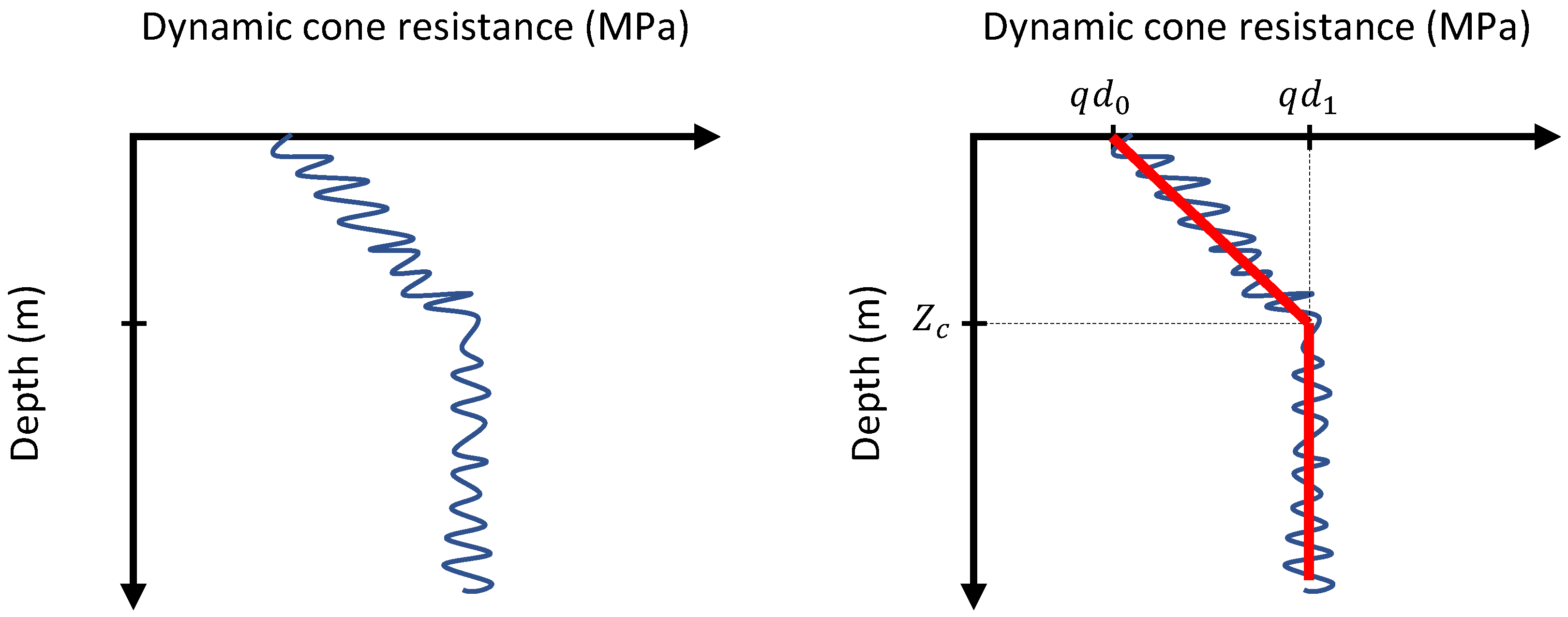
A key requirement for the practical use of the LDCP is a calibration phase, which must be carried out for each soil type under known laboratory or field conditions of density and moisture content (W) [38]. The calibration process involves generating a reference penetrogram in the –z domain. Figure 1(left) illustrates such a raw signal for a homogeneous granular soil, while Figure 1(right) highlights the three characteristic parameters extracted from it [38]. These are as follows: (i) the initial resistance , which reflects near-surface conditions; (ii) the stabilized resistance , representing deeper, steady-state behavior; and (iii) the transition depth , which marks the shift between the two regimes. Together, these parameters define a reference curve for the soil, and this curve is later used to establish acceptance and rejection thresholds for compaction control in situ.
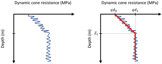
Figure 1.
(left) The raw penetrometric signal in the –z space for a homogeneous granular medium. (right) Characteristic parameters of the reference curve (, , and ).
At present, data processing and interpretation are handled through the online platform Websprint. Websprint allows users to manage and compare reference curve databases [38], apply acceptance or rejection criteria consistently, and produce standardized reports. In practice, this digital environment has made it possible to use LDCP results in real time, facilitating both on-site decision making and long-term documentation of compaction performance.
- (e.2)
- DCP-Standard penetrometer. The dynamic cone penetrometer, in its standard configuration (DCP-Standard), is widely recognized as a practical tool for in situ control compactation. The test is standardized under ASTM D6951 [6]. It employs an 8 kg hammer dropped freely from a height of 575 mm onto a 60° conical tip with an area of 4.04 cm2. The primary outcome is the penetration index (DPI, expressed in mm/blow) or, alternatively, its reciprocal (blows/mm).
These indices can be correlated with design and performance parameters, such as the CBR index, the resilient modulus, and shear strength properties [39,40,41]. Because of frictional effects along the rods, the penetration depth is typically limited to about 1 m. The device is most suitable for soils or granular bases with a low percentage of particles larger than 50 mm, where consistent penetration can be achieved.
The DCP-Standard is generally considered an economical and accessible method for QA control. In practice, however, its use requires two operators: one to carry out the test and another to record depth readings. Furthermore, results may show some dependence on operator technique, highlighting the importance of consistent procedures in the field.
- (e.3)
- DCP-Utility penetrometer.
The DCP-Utility is essentially a lighter version of the standard device, created specifically for layer-by-layer QC. It works with a 2.3 kg hammer dropped from a height of 508 mm onto a 25° cone tip with an area of 4.84 cm2. The test records the average number of blows, N, needed to penetrate increments of 83 mm. This tool is standardized under ASTM D7380 [42] and is well-suited for fine soils, base layers, and shallow fills up to about 0.16 m in depth. Its main strengths are simplicity and low cost, making it a practical option for routine quality checks. However, its use becomes more limited in cemented soils or in materials containing particles larger than 37 mm.
- (e.4)
- PANDITO penetrometer. The PANDITO is a lightweight, constant-energy penetrometer with a 5 kg hammer dropped from 610 mm onto a 90° conical tip of 2 cm2. Results are expressed as the penetration index (DPI) or its inverse, corresponding to the number of blows required to advance 25.4 mm. The device reaches a maximum depth of about 0.5 m and is mainly used for the QA of shallow compacted layers. Its results can be related to CBR and the resilient modulus, but reliable use requires prior calibration and field experience, as testing usually involves at least two operators.
- (e.5)
- Dynamic cone penetrometer. The Dynamic Cone Penetration Test (DCPT) is a heavy constant-energy device used for subsurface exploration and quality assurance at greater depths. It consists of a 63.5 kg hammer dropped from 750 mm onto a 50 mm rod train fitted with a 60° conical tip of 44.8 cm2. Test results are commonly reported as the number of blows per 300 mm of penetration, which can also be converted into a dynamic tip resistance . With a penetration capacity of up to 15 m, the DCPT is widely applied to fine granular soils and is often used in liquefaction assessment. While it provides robust information at depth, field operation is slower, more expensive, and typically requires a larger crew; results may also be affected by hammer efficiency and rod alignment [43,44,45].
- (e.6)
- Comparative technical summary. The following tables provide a clear overview of the most relevant differences among the dynamic penetrometers considered in this study:
- Equipment (Table 2): The LDCP is the only device operating with variable energy, and it offers more detailed insight by allowing penetration to be interpreted as a function of the applied energy. Hammer weights vary considerably across devices, from as little as 2 kg for the LDCP to as much as 63.5 kg for the DCPT.
 Table 2. The equipment characteristics of LDCP, DCP-Utility, DCP-Standard, PANDITO, and DCPT.
 - Operation (Table 3): With the exception of the DCPT, all penetrometers require calibration. The LDCP is distinctive in that it demands a reference calibration based on the parameters , , and . In practice, this calibration is supported by curated databases accessible through the Websprint platform, which ensures higher repeatability and minimizes operator dependence compared with manually read devices, such as the DCP-Standard or the DCP-Utility.
 Table 3. Operational characteristics of LDCP, DCP-Utility, DCP-Standard, PANDITO, and DCPT.
 - Application (Table 4): Among the instruments reviewed, the LDCP is the only one that can be used reliably for both QC and QA. In QA mode, the LDCP can reach depths of up to 6.0 m, clearly outperforming the DCP-Utility (0.16 m), the PANDITO (0.5 m), and the DCP-Standard (1.0 m). While the DCPT is capable of penetrating as deep as 15 m, its use is logistically demanding, requires multiple operators, and is not suited for routine compaction control.
 Table 4. Applications of LDCP, DCP-Utility, DCP-Standard, PANDITO, and DCPT.
 - Standards (Table 5): The DCP-Standard (ASTM D6951) and DCP-Utility (ASTM D7380) are mainly intended for shallow pavement layers. By contrast, the LDCP is covered by the French standard NF P 94-105, which applies not only to pavements, but also to compacted fills and natural subgrades, explicitly covering both QC and QA applications. The DCPT, on the other hand, is regulated under NF P 94-063, a standard focused on deep soil profiling rather than compaction control.
 Table 5. Summary of standards for dynamic penetrometers in compaction control.
- (iii)
- Intelligent compaction (IC).
Intelligent compaction equips vibratory rollers with accelerometers and Global Navigation Satellite System (GNSS) receivers to produce continuous compaction control (CCC) maps and stiffness-based IC measurement values (ICMVs). IC greatly improves coverage and process control; typical practice calibrates ICMVs against spot tests (density, LWD, and DCP) on a test strip before production [30,31,34]. The moisture, stress state, and underlying layers influence ICMVs, so most agencies still pair IC with verification testing [31].
- (iv)
- Remark on data-driven control.
A recent work has explored machine learning models to predict compaction parameters and QC indicators directly from soil descriptors and field signals, potentially reducing the testing effort while improving uniformity [16].
2.3. Related Work
To contextualize this study, the literature was synthesized into six thematic clusters: (1) classical QA/QC for compaction; (2) dynamic penetrometers for compaction control; (3) intelligent/continuous compaction control; (4) data-driven and ML prediction of in situ resistance or acceptance metrics; (5) explainable ML in geotechnics; and (6) standards and specifications.
- (i)
- Classical QA/QC for compaction (density-, stiffness-, and penetration-based).
Field acceptance has historically relied on achieving a percentage of the laboratory () determined by SPC or MPC tests, with control of water content around the () [1,2,3,32,33]. In situ verification has been implemented primarily with the sand cone and nuclear gauge methods; the rubber-balloon method appears in legacy practice but was withdrawn in 2024 [4,5]. These density-based spot tests are robust but spatially sparse. Stiffness-oriented methods, such as static plate load (/) per DIN 18134 and portable impact/deflection devices (LWD/PFWD), provide performance-related metrics and have been adopted to complement density checks [7,8,9]. Comparative studies show reasonable trends between the density, deflection-derived modulus, and CBR index, with moisture- and gradation-dependent scatter [11,31,46]. Take away: density tests provide traceable compliance to lab benchmarks but limited coverage; stiffness and penetration offer performance-relevant checks that benefit from local calibration.
DCP and LDCP (Panda; EN ISO 22476-2 classes DPL/DPM/DPH) provide fast resistance profiles with depth, enabling the detection of weak lenses and stratification in compacted layers [6,10]. Numerous field and laboratory studies report the correlations between DCPT or LDP indices and the CBR index, modulus, and shear strength; for sands and granular fills, logarithmic or power-law forms are common [11,46,47]. Moisture (W) exerts a strong influence—penetration resistance typically decreases when compacted and wet, —consistent with observations in lateritic and fine-grained soils [48]. Instrumented LDPs report the with improved resolution for softer materials and continuous profiles; in this context, the near-surface and stable-depth indices and are used in practice and were also used in this study (note that these indices are specific to instrumented LDPs such as LDCP and are not reported by the ASTM DCP). Energy-based analyses highlight the influence of the hammer energy transfer and shaft vibrations on derived indices [13]. Penetrometer results are sensitive to moisture state, oversized particles, and fabric; energy standardization and consistent procedures improve repeatability. Compared to density tests, penetrometers increase vertical resolution and productivity, but acceptance thresholds typically require local calibration to laboratory references or modulus-based criteria [6,10].
- (ii)
- Intelligent compaction (IC) and continuous compaction control (CCC).
IC-equipped rollers report an intelligent compaction measurement value (ICMV) that reflects composite near-surface stiffness under vibratory loading, producing continuous spatial coverage of compaction quality. Field comparisons show that ICMV trends align with spot stiffness and strength indicators (e.g., and DCP penetration), while moisture and underlying layer effects introduce scatter [30,34]. Reviews emphasize IC as a process control tool to homogenize compaction and reduce testing blind spots; calibration on test strips against point tests remains essential for setting project-specific thresholds [30,31,34]. Take away: IC/CCC improves spatial coverage and process feedback; acceptance typically combines IC mapping with limited spot verification (e.g., LWD and DCP).
- (iii)
- Machine learning for predicting the in situ strength or compaction outcomes.
Data-driven models have been increasingly used to estimate compaction-relevant properties from readily available descriptors (grain size indices, Atterberg limits, moisture and density states, and binder contents for treated soils). In expansive and treated soils, Gaussian process regression (GPR) and ensemble methods have been shown to predict the soaked CBR index with high accuracy using limited but well-curated datasets, thereby offering rapid proxies to time-consuming laboratory tests [15]. For borrow-source screening and design targeting, ensemble models (Random Forest, XGBoost) have been reported to predict the Proctor parameters (, ) of expansive soils with an above 0.9, highlighting the value of the nonlinear feature interactions between plasticity, FC, and compaction energy [16]. For performance-oriented acceptance, ML has been applied to stiffness surrogates: the resilient modulus of compacted subgrades has been predicted using ensemble learners (bagging/boosting over trees and k-NN), and it has been compared against neural models, with external validation across stress states [17]. Similar trends have been confirmed for cementitiously stabilized subgrades, where SVM, ANN, and GPR models capture the stress- and moisture-dependence of beyond linear correlations [18]. Typical sample sizes range from to observations; reported limitations include site-specific bias and reduced extrapolation when moisture or gradation fall outside the training domain. Take away: ensemble and kernel methods provide accurate surrogates for the CBR index///, but generalization depends on broad, well-stratified datasets and consistent feature spaces.
- (iv)
- Explainable ML (XAI) in geotechnics.
Interpretability has been adopted to assess whether ML decisions are consistent with soil mechanics. SHAP-based analyses have been used to rank physical drivers and expose the nonlinear effects in stabilized soils; for example, geopolymer-treated clays have shown feature attributions aligned with expectations (binder type/content increasing UCS; higher plasticity reducing it) [23]. For hazard-type classification tasks, an XGBoost–SHAP framework for liquefaction potential has provided global and local explanations, identifying penetration resistance and fines as dominant contributors and flagging class-imbalance remedies (SMOTE) as influential to model stability [49]. Beyond case studies, recent methodological critiques have proposed evaluation structures combining performance metrics with domain plausibility checks and data/algorithm audits, advocating routine use of tools such as SHAP to verify monotonic trends (e.g., density ↑⇒ strength ↑) and to detect spurious shortcuts [24]. Take away: SHAP/TreeSHAP has matured as a practical audit layer for tree/ensemble models; embedding physical plausibility and data diagnostics alongside accuracy improves trust and facilitates specification uptake.
- (v)
- Standards, guidelines, and specifications.
Laboratory references for acceptance are codified in ASTM/AASHTO and EN standards, which define the Proctor procedures and field density methods that underpin percentage-compaction criteria [1,2,3,4,5,32,33]. Dynamic probing procedures (EN ISO 22476-2, with Amendment 1) and the ASTM DCP standard provide consistency and energy normalization for penetration-based control [6,10]. European practice references modulus-based control via plate load and LWD/PFWD correlations for unbound layers [7,8,9]. Implementation guidance for IC emphasizes calibration with point tests before production [30,31]. Take away: specifications are evolving from density-only acceptance toward complementary stiffness and penetration criteria, with standardized procedures enabling traceability and calibration across methods.
- (vi)
- Rationale for emphasizing dynamic penetrometers in this study.
Dynamic penetrometers offer rapid, low-cost, and portable profiling of resistance with depth, yielding dense spatial information compared with sparse density tests. The lightweight/instrumented class provides indices () that are sensitive to both density and moisture state—primary drivers of compaction performance—and can be consistently standardized under EN ISO 22476-2 and ASTM D6951 [6,10]. Given these properties and their empirical links to the CBR index/modulus, the penetrometric indices and are natural targets for prediction and interpretation in ML workflows aligned with field logistics.
3. Materials and Methods
3.1. Database
A database was assembled from field compaction control campaigns performed with a LDCP and from companion laboratory tests. Records were drawn from several construction materials that covered a broad grain size spectrum, including gravelly fills and sands (e.g., site gravel; rolled or crushed gravels in the ranges 4/8, 6/10, and 10/20 mm; and a calibration sand). For each record, a soil class under the GTR system (Guide des Terrassements Routiers) [50] was registered (e.g., D2, DC1, DC3, and B2), and a Unified Soil Classification System (USCS) [51] label was included when available. A site identifier (Nom_BDD) was stored to allow grouping by origin during validation. A graphical overview of the soil-type coverage is provided in Figure 2.
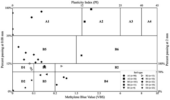
Figure 2.
GTR classification map of the observations in the database. The diagram is defined by the VBS on the horizontal axis, the percent passing at 0.08 mm (FC) on the left vertical axis (0–100%), the percent passing at 2 mm on the right vertical axis (70–100%), and the PI on the top axis. Symbols identify the soil types A1–A4, B1–B6, and D1–D2, with sample counts in parentheses.
The following families of variables were recorded for every observation, depending on availability:
- Grain-size descriptors: key indicators derived from standard sieve and hydrometer analyses. These include the characteristic diameters , , , and , which correspond to the particle sizes at which 10%, 30%, 50%, and 60% of the soil mass passes through the gradation curve. The maximum particle size and the full cumulative passing distribution were also taken into account. In addition, the relative fractions of gravel (G), sand (S), and fines (F) were considered to describe the overall soil texture. Whenever possible, classical gradation coefficients were computed, including the coefficient of uniformity (), the coefficient of curvature (), and, where relevant, the high-plasticity clay index (). Taken together, these descriptors provide a consistent framework to capture both the spread and the shape of the particle-size distribution.
- Plasticity and fines activity: parameters describing the consistency and surface activity of fine-grained soils. The Atterberg limits include the liquid limit () and the plastic limit (), from which the plasticity index () is derived. These indices provide insight into the soil’s water retention capacity, workability, and its tendency to undergo volumetric changes. In addition, the methylene blue value () was considered an indicator of the surface activity of clay minerals. This parameter reflects both the quantity and the reactivity of the clay fraction, complementing the Atterberg limits by providing information on the adsorption properties and potential sensitivity of the fines.
- State variables: descriptors of the in situ condition of the soil. These include the natural water content (W), expressed as a percentage of the dry mass, and the dry unit weight (). Together, these parameters provide a direct measure of the balance between moisture and density that governs soil performance.
- Compaction references: parameters derived from the SPC test are used. These include the and the maximum dry density . Based on and , the percentage is obtained.
- Penetrometric responses: in situ indices and obtained with a lightweight dynamic cone penetrometer (LDCP). The parameter represents the dynamic cone resistance recorded at or near the surface, while corresponds to the stabilized resistance reached once the soil becomes confined at depth. This transition occurs at a critical depth , beyond which the resistance tends to remain constant. These values were determined consistently for all cases included in the database.
Heterogeneous naming from the original sheets was harmonized, and decimal commas were converted into decimal points. Basic consistency checks were applied to remove duplicate rows and physically impossible entries. For modeling, the regression target was . Records with missing target values were excluded, while missing feature values were handled by median imputation inside the learning pipelines. Continuous features were standardized when required by the estimator. To enable later assessment of generalization across sites or materials, the Nom_BDD and GTR fields were retained for grouped resampling schemes.
Each row in the database corresponds to a unique set of measured or derived properties associated with field and laboratory data. While multiple records may originate from the same work front or construction site, the combination of attributes recorded for each is not an exact copy of any other. Differences can occur in one or several variables—for example, in gradation, plasticity, water content, dry density, or compaction reference values—reflecting real spatial and material variability within the works. Repeated entries and exact duplicates were removed during quality control, and heterogeneous naming was harmonized as described previously. Under this structure, the records are treated as distinct observations for modeling purposes.
Although multiple tests can originate from the same work front or site, the input vectors associated with individual records differ because they reflect the specific soil state and characterization at each test point. This heterogeneity is expressed through variations in gradation descriptors (e.g., , , , , and ), plasticity/activity indicators (, , , and ), in situ conditions (W and ), and compaction references (e.g., , and ). In practice, tests performed within the same site often exhibit different moisture contents, densities, and even GTR/USCS classifications due to lift-to-lift variability, changes in borrow sources, and adjustments in construction processes. This variability constitutes the record-level diversity that is captured by the learning algorithms.
A site identifier (Nom_BDD) is stored to characterize the grouping structure and to enable group-aware resampling schemes. Several GTR/USCS soil classes are represented at only one site in the current database. This distribution creates a partial confounding between site and class: for those classes that occur exclusively at a single site, the removal of that site would imply the simultaneous removal of all training data for those classes, effectively transforming the task into extrapolation to unseen soil types rather than evaluation of cross-site generalization for shared classes. Under this structure, applying a global leave-one-site-out (LOSO) scheme would simultaneously test for site transfer and for class deletion. To avoid this confounding, the primary evaluation is based on a fixed 80/20 random hold out that preserves class coverage in both training and testing partitions, with the random seed shared across model families to ensure comparability. The site identifier is retained only for diagnostic purposes and for the design of optional group-aware sensitivity checks on subsets where at least two sites share the same GTR class.
The full dataset comprises 360 records distributed across multiple GTR soil classes, covering a broad range of compaction behaviors. Table 6 summarizes the number of records per class. The most frequent classes are B5 (101 records) and A1 (90 records), followed by B4 (32) and A2 (26). Less represented classes include D1, B2, B6, DC3, B3, D2, B1, and DC1, each with fewer than 20 observations. This distribution provides good coverage of the coarse (A-family) and fine-grained (B- and D-family) materials typically encountered in earthwork projects.

Table 6.
Distribution of records by GTR soil class.
The coverage of soil types is visualized in the GTR diagram in Figure 2. Each observation was positioned by its VBS, PI, and fines contents at 0.08 mm and 2 mm. A broad span across the A-, B-, and D-families was observed, indicating that both low- and high-plasticity ranges and a wide spectrum of fines contents were represented. This graphical check was used to confirm that the database captured typical field materials used for earthworks and to support later grouped resampling by GTR class.
3.2. Supervised Learning Methods for Penetrometric Response
Short descriptions of the learning techniques are provided below. Only defining ideas and distinctive equations, without detailed derivations, are included. Model selection was aligned with the data structure and the prediction task. The inputs are fixed-length tabular predictors (gradation, plasticity/activity, in situ density and moisture, and Proctor references), and the targets are scalar LDCP indices (, ) or , so the features do not carry intrinsic temporal or positional order. Under this setting—small-to-medium sample sizes, heterogeneous tabular variables, and scalar outputs—regularized linear models, SVR, tree ensembles (Random Forest, XGBoost), and a compact feed-forward MLP are strong, data-efficient choices whose behavior can be audited with SHAP. Sequence architectures (LSTM, GRU, and Transformers) add complexity and typically require larger sequential datasets to realize their advantages; they are more appropriate when learning depth- or time-resolved signals (e.g., full profiles or CCC/IC time series) or when explicit positional dependencies are present. For this reason, tabular learners were prioritized here, and sequence models are left as a future extension if depth/time series are incorporated.
- Ridge regression.
A linear predictor was fitted under the squared loss with an penalty to stabilize coefficients under collinearity:
with .
- Lasso.
An penalty was used to promote sparsity (embedded selection):
- Elastic net.
A convex combination of and penalties balanced sparsity and stability:
with mixing parameter .
- Support vector regression (SVR).
The -insensitive loss enforced a flat function with controlled deviations:
with kernel predictor
- Random Forest.
An ensemble of decision trees was grown on bootstrap samples with random feature subsetting at each split; predictions were then averaged:
Splits maximized the reduction in variance:
- Gradient boosting with trees.
An additive model was built stagewise to follow the negative gradient of the loss:
where is a shallow tree fitted to pseudo-residuals , is a line-search weight, and is the learning rate.
- Feed-forward neural network (MLP).
A fully connected network with L layers modeled smooth nonlinear mappings:
with activation (ReLU or tanh). Parameters were obtained by minimizing MSE with weight decay and early stopping. Inputs were standardized.
- Common preprocessing and tuning.
All models were embedded in identical pipelines with median imputation. Standardization was applied when required (SVR and MLP) and skipped for tree-based models. Hyperparameters (e.g., , , C, tree depth, and learning rate) were selected by cross-validation to ensure fair comparison.
3.3. Modeling Pipeline and Evaluation
A single, reusable pipeline was applied to all models. The primary analysis focused on for the formal train–test evaluation, and additional models were fit for and to support comparative plots and SHAP explanations. The set of predictors is listed in Table 7. Missing values were imputed by the median. Standardization was applied to models that are scale-sensitive (linear models, SVR, and MLP) and skipped for tree-based models (Random Forest, XGBoost). A stratified procedure was not required because the outcome is continuous; instead, a random 80/20 train–test split was used with a fixed seed for reproducibility. Model families and their search spaces are summarized in Table 8. Error metrics were computed as defined in Table 9.

Table 7.
The model inputs used in all experiments (standardized symbols).

Table 8.
Hyperparameter grids (summary of key ranges).

Table 9.
Error metrics: definitions and goals. n is the number of samples, are the true values, are the predicted values, and is the sample mean of the true values.
Training and inference were negligible in this study due to the small dataset (). All models were trained in under 4 s on a standard laptop (Intel i9, 64 GB RAM) using CPU implementations (scikit-learn/XGBoost), and the test time prediction was virtually instantaneous. Computational cost did not constrain model selection or evaluation.
Algorithm 1 summarizes the end-to-end process. Grid search with 5-fold cross-validation was used inside the training set and optimized the negative RMSE. The best configuration per family was refit on the full training split and evaluated on the held-out test split. In addition to test metrics, a manual 5-fold cross-validation of the selected pipeline was computed on the entire dataset to report the mean ± SD for all metrics. For linear models, coefficients were exported when available. For the tree-based models, impurity-based feature importances were exported. For the final boosting model, global and local explanations were produced with SHAP (TreeExplainer), including the mean importances, a beeswarm plot, and top-N dependence plots, along with tabular exports.
All steps in Algorithm 1 correspond to the provided code: median imputation, optional standardization, grid searches in Table 8, metrics in Table 9, CSV artifact exports (e.g., predictions, residuals, and run logs), and the feature set in Table 7. The same random seed and split ratio were used across families to enable fair comparison.
| Algorithm 1 Modeling and evaluation pipeline |
|
Linear baselines (OLS, Ridge, Lasso, and Elastic Net) establish the transparent reference performance and quantify the linear signal with and without shrinkage. SVR with several kernels captures nonlinear structures with margin control. A feed-forward MLP acts as a generic nonlinear function approximator with early stopping. Random Forest (RF) and XGBoost (XGB) are strong, regularized ensemble learners with built-in handling of complex interactions and monotone trends; their grids (Table 8) were intentionally compact to limit overfitting to validation folds.
The RMSE was minimized during tuning because it aligns with the squared-error objectives used by linear and boosted-tree models. Final comparisons across families were reported using , MSE, RMSE, and MAE, as defined in Table 9. The same train/test split and cross-validation protocol were applied to all families to ensure fairness. This strategy was chosen because each sample represents independent compaction and moisture conditions, which helps reduce the chance of information leakage between training and testing. At the same time, we acknowledge that grouped validation could offer useful insights into site-specific effects, especially when larger and more balanced datasets are available.
For linear models, standardized coefficients were reported when applicable. For RF and XGB, impurity-based importances were exported for global ranking. SHAP was used to provide consistent, model-agnostic attributions on the final XGB pipeline: the mean ranked variables globally, the beeswarm summarized feature effects, and the dependence plots illustrated main effects and interactions.
As an additional statistical reference, we implemented a simple GTR-average predictor. In this baseline, each observation was assigned the mean value of (or , ), corresponding to its GTR soil class (e.g., A1, A2, B5, etc.). This baseline reflects a naïve approach that relies solely on soil classification without considering density, moisture, or gradation descriptors. The comparison with machine learning models highlights how much predictive accuracy is gained when these state and material descriptors are incorporated.
4. Results Obtained
4.1. Model Comparison
The GTR-average baseline achieved only and RMSE , confirming that soil class alone carries minimal predictive information for .
The mean absolute percentage error (MAPE) was included to provide a relative measure of error expressed as a percentage, which is particularly useful for comparing model performance across different scales. The Pearson correlation coefficient (R) complements by capturing the strength and direction of the linear relationship between predictions and observations. High values of R indicate a strong linear association, even when is modest.
The test performance for is summarized in Table 10. The MLP achieved the best fit (, RMSE ), followed by XGB (, RMSE ), whereas the RF and SVR exhibited larger errors (RMSE and , respectively). In relative terms, the RMSE of MLP was lower by approximately compared with XGB, compared with RF, and compared with SVR, indicating a consistent advantage of MLP on the held-out test set (Table 10).

Table 10.
Test set performance (qd1). , RMSE, MAE, and MSE reported by model.
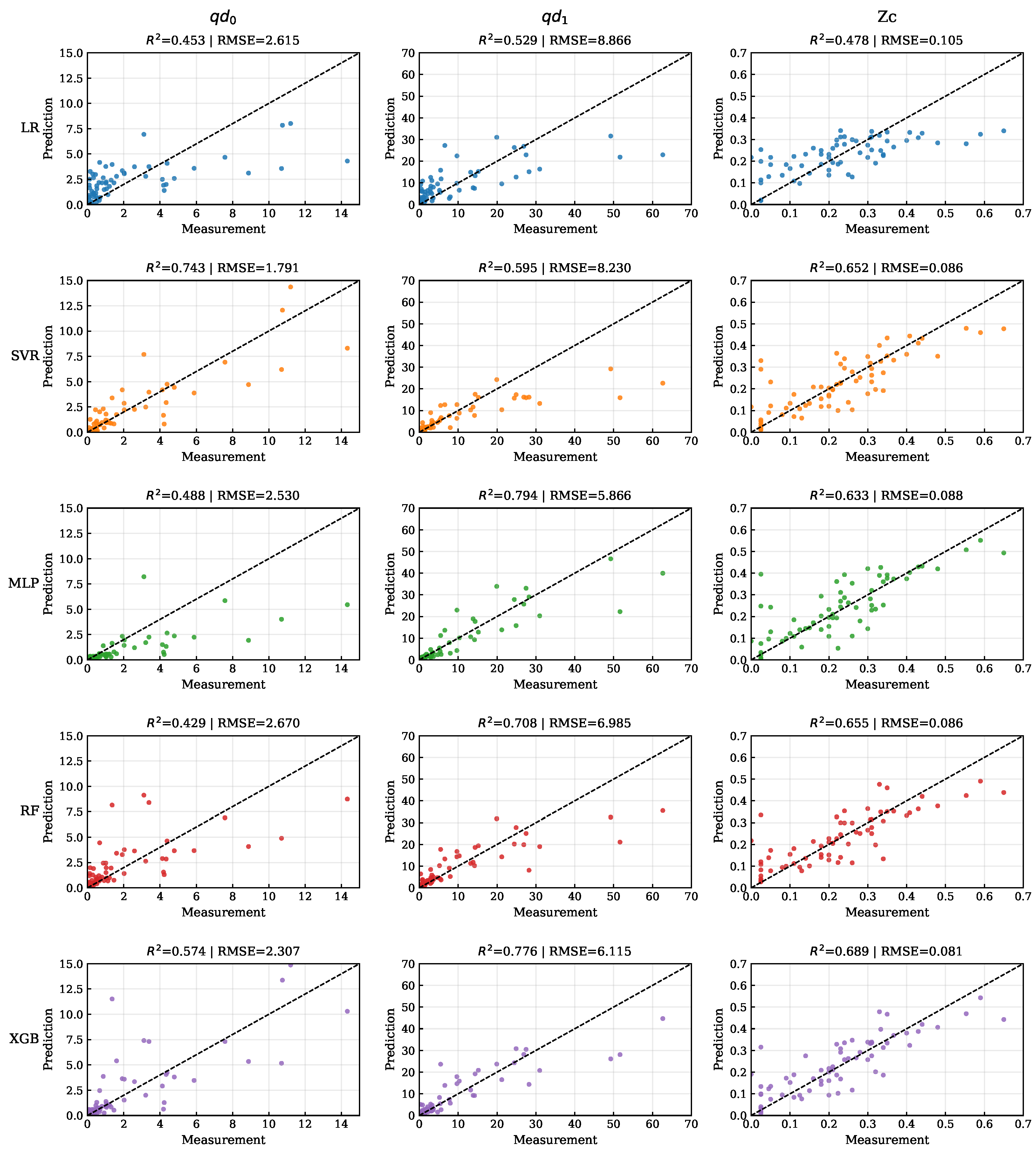
The prediction–measurement scatter across targets and models is displayed in Figure 3. Linear baselines are shown for qualitative reference; the summary tables focus on the four best-performing families. Point clouds were observed to lie close to the identity line, with tighter clustering for MLP and XGB. A mild underestimation at the upper tail of qd1 was visually apparent, which is further examined through calibration analysis in the statistical validation subsection.
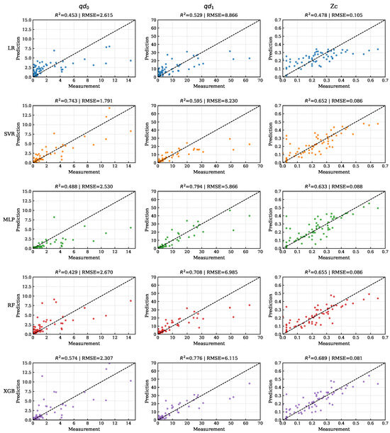
Figure 3.
The prediction–measurement scatter for , , and across model families. The dashed line indicates the identity (1:1); panel headers report the and RMSE.
Five-fold cross-validation results (Table 11) were consistent with the test set ranking. The MLP attained the lowest average error (RMSE ) and the highest mean (). XGB and SVR presented similar mean values (0.716–0.722), while SVR and RF showed larger fold-to-fold variability (RMSE standard deviations of 1.94 and 1.78), suggesting greater sensitivity to data partitioning.

Table 11.
Five-fold cross-validation (). The test statistics and mean ± SD are shown below each metric.
Because several differences were modest (for example, MLP versus XGB), a formal assessment with bootstrap uncertainty, paired comparisons with multiplicity control, and calibration statistics is reported in the next subsection.
A CPU benchmarking procedure was conducted to evaluate the computational cost of training and the single-sample inference latency of the final models (MLP, XGBoost, Random Forest, and SVM). A warm-up fit–predict cycle was first performed to minimize cold-start effects. Each model was subsequently retrained from scratch seven times in order to estimate the mean and standard deviation of the training time. Single-sample inference latency was measured using 400 repeated one-row predictions with fixed random indexing, while single-thread execution was enforced when applicable to ensure comparability.
Detailed per-trial timings were stored in CSV files ({MODEL}_fit_runs.csv and {MODEL}_predict_1sample_runs.csv), and summary statistics were compiled in a Timings.csv file containing system metadata.
The resulting training times and latencies are presented in Table 12. Training was found to be inexpensive for all models, with SVM exhibiting the lowest mean training time (0.008 s), followed by XGBoost (0.108 s), MLP (0.356 s), and Random Forest (3.258 s). Inference latency for a single sample was below 2 ms for all models except Random Forest, which showed a markedly higher latency of 58.5 ms.

Table 12.
The training time and single-sample latency for each model. Training time is reported in seconds; latency is reported in milliseconds. Values represent the mean ± standard deviation over multiple runs.
These results indicate that MLP and XGBoost achieved strong predictive performance while maintaining low computational overhead, making them suitable for real-time deployment and rapid model retraining workflows. In contrast, the higher inference cost of Random Forest may limit its applicability in latency-critical contexts.
4.2. Calibration, Residuals, and Prediction Intervals
Calibration and uncertainty were evaluated as part of the model performance analysis. Calibration was assessed by regressing the observed values on predictions in the test set and by examining residual diagnostics and residual distributions [52]. These diagnostics provide complementary perspectives: the calibration regression quantifies systematic biases (through slope and intercept), while the residual plots allow for the visual inspection of deviations from ideal behavior.
Prediction-level uncertainty was quantified through split-conformal prediction intervals, where a model-agnostic procedure with finite-sample coverage guarantees under the exchangeability assumption [53,54]. In this approach, the training set is split into two parts. The first subset is used to fit the model, while the second subset (the calibration set) is used to compute the nonconformity scores as the absolute residuals between predicted and observed values. The quantile of these scores is then used to build symmetric intervals of the form for each new prediction. This construction provides distribution-free uncertainty quantification without assuming specific error models.
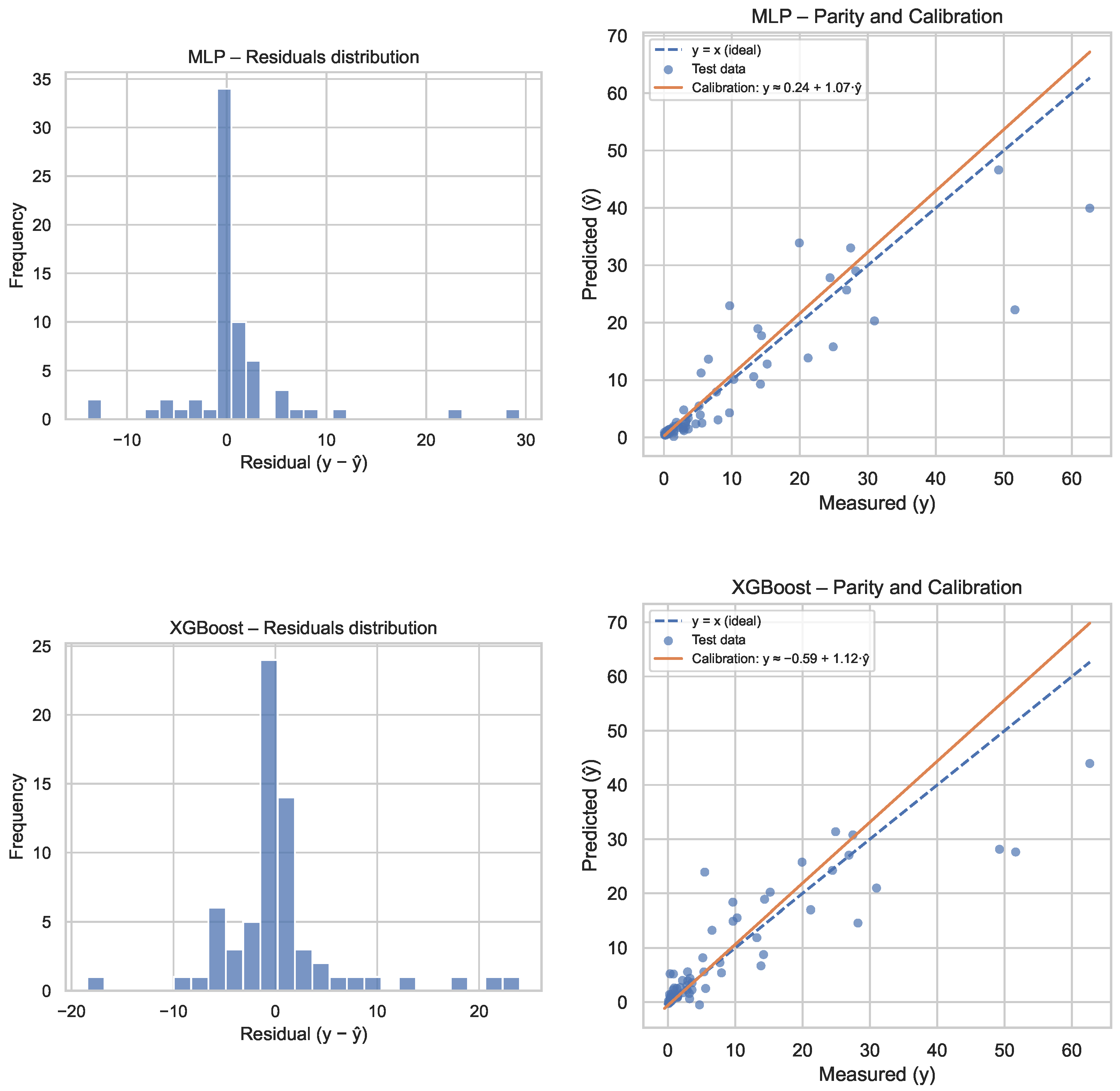
Figure 4 summarizes the calibration and residual diagnostics for both XGBoost (top row) and MLP (bottom row). The left column shows the residual distributions, which are useful for inspecting dispersion and asymmetry, while the right column presents parity plots with fitted calibration lines compared against the ideal line. The calibration slopes and intercepts were close to the ideal values, indicating reasonable agreement between the predicted and observed responses. Residual plots displayed limited structure overall, although some heteroscedasticity was visible at higher predicted values.
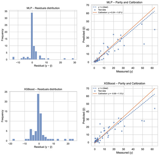
Figure 4.
Summary of the calibration and residual diagnostics for XGBoost (top) and MLP (bottom). Left: residual distributions. Right: parity plots with fitted calibration lines compared to the ideal line.
For XGBoost, the absolute-residual quantile at was , resulting in prediction intervals of the form . The empirical coverage on the test set was (target ), which indicates undercoverage under this simple, global construction. This undercoverage is likely due to residual heteroscedasticity and differences between calibration and test data distributions. For MLP, the corresponding quantile was with an empirical coverage of , which was closer to the nominal target. The lower bounds of these intervals can be directly compared with compaction acceptance thresholds, providing a transparent and statistically grounded basis for QA/QC decisions in the field.
A simple but robust QA/QC procedure can be derived directly from the calibrated models and their conformal prediction intervals. For each new test location, the model prediction and its prediction interval are computed. The lower and upper bounds of this interval are then compared with the acceptance threshold T defined by the compaction specification (e.g., the required value).
The following rule is then applied. If the lower bound of the interval is above T, the location is accepted with an estimated error rate of, at most, under the exchangeability assumption. If the upper bound is below T, the location is rejected. If T lies inside the interval, the result is classified as a “gray zone” and additional on-site verification (e.g., density or penetrometer testing) can be carried out. This three-way decision rule connects the statistical model to operational QA/QC decisions in a transparent way.
Practical error rates can be estimated on the test set by comparing predictions and intervals against observed values. False acceptance is defined as the proportion of cases where the lower bound is above T but the true value is below T. False rejection is defined analogously. These rates provide a clear picture of how often decisions based on model predictions would differ from those based on measured values, and they can be adjusted by selecting or adding a safety margin to T.
This framework provides a principled way to translate statistical calibration and uncertainty quantification into field decisions. Because the conformal intervals have finite-sample coverage guarantees, the resulting acceptance and rejection decisions have a quantifiable risk that can be explicitly reported and controlled, rather than relying on ad hoc safety factors.
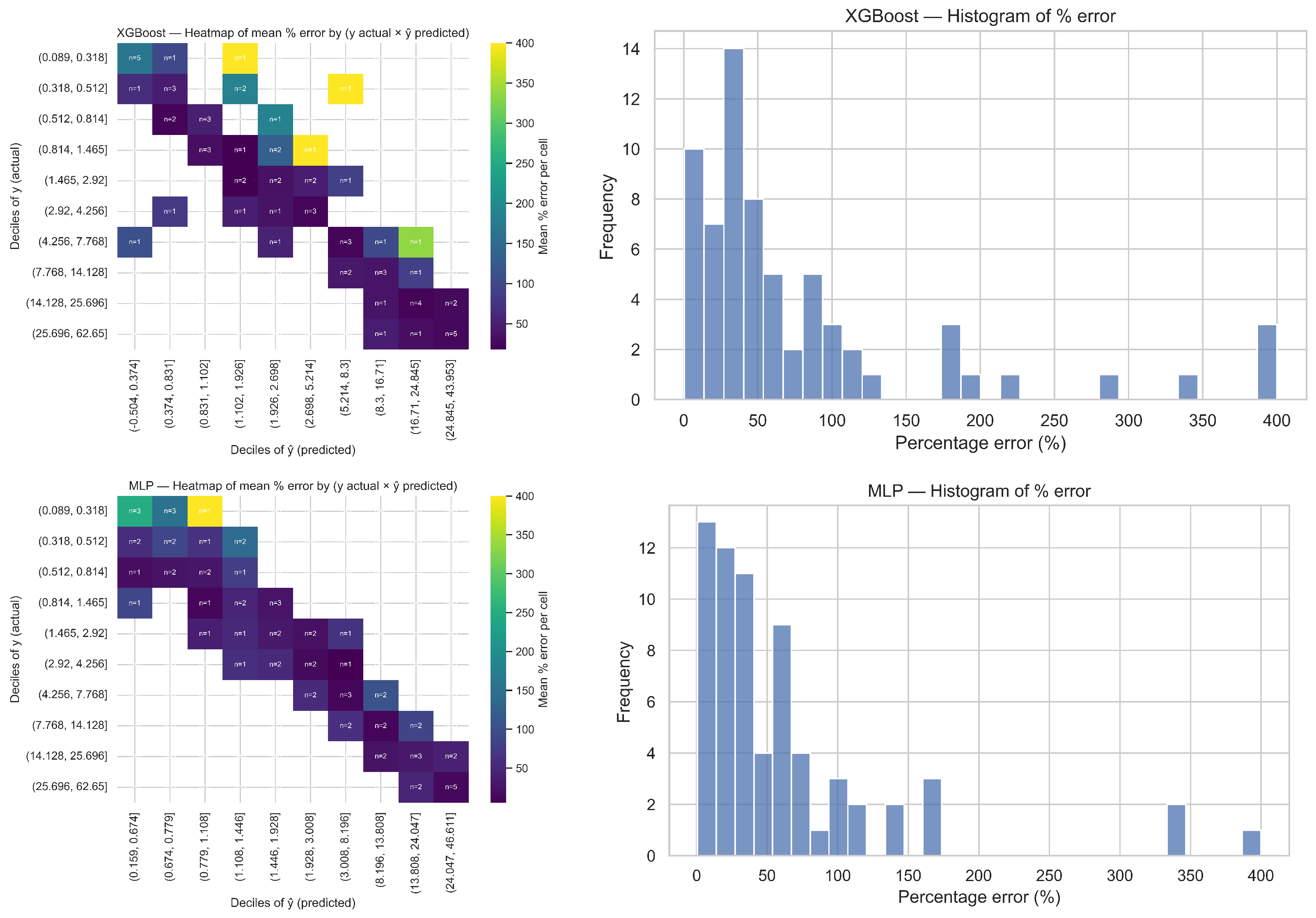
To complement the calibration and conformal analysis, the models were also evaluated using percentage errors (MAPE-style), which were defined as . This relative metric enables a direct comparison of performance across different ranges of the target variable. Two complementary visualizations were used for this analysis: heatmaps of the mean percentage error stratified by deciles of y and , and histograms of the percentage error on the test set. These are shown in Figure 5 (page 1), with XGBoost in the top row and MLP in the bottom row.
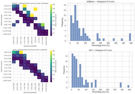
Figure 5.
Percentage-error analysis (MAPE-style) for XGBoost (top) and MLP (bottom). Left: heatmap of the mean percentage error by deciles of y (actual) and (predicted), annotated with sample sizes. Right: histogram of the percentage errors on the test set.
The heatmaps display how the relative error varied jointly across actual and predicted deciles, with each cell reporting the mean percentage error and being annotated with the corresponding sample size n. For XGBoost, the lowest errors were concentrated along the diagonal, indicating reasonable calibration for mid-range values. A few yellow cells, corresponding to the highest percentage errors, are located in the upper central region of the heatmap. These cells are associated with small values of y and higher predicted deciles, reflecting over-prediction in the low-value regime. Their sample sizes are very small (), which makes their mean values less stable but still highlights systematic patterns worth noting. The histogram supports this interpretation: most errors are moderate, but a long right tail remains, with some extreme values reaching approximately 300–400%. These large relative errors occur mainly when the denominator y is small.
In the case of MLP, the heatmap exhibits a more uniform pattern overall. The diagonal is consistently cool, and only one yellow cell is present (first row, third column), again associated with small-y values. High-error, off-diagonal cells were less frequent than in XGBoost, and the histogram shows a clear leftward shift, with a larger proportion of predictions displaying lower percentage errors. Although a tail of high relative errors persisted, these were isolated and mostly linked to very small denominators.
Taken together, these visualizations indicate that both models perform well in mid-range regimes, while relative errors increase for small values of y, particularly when predictions overshoot. Compared to XGBoost, MLP shows a tighter distribution of percentage errors and a more stable heatmap structure, suggesting greater robustness on a relative scale.
4.3. Variable Importance and Model Explanations
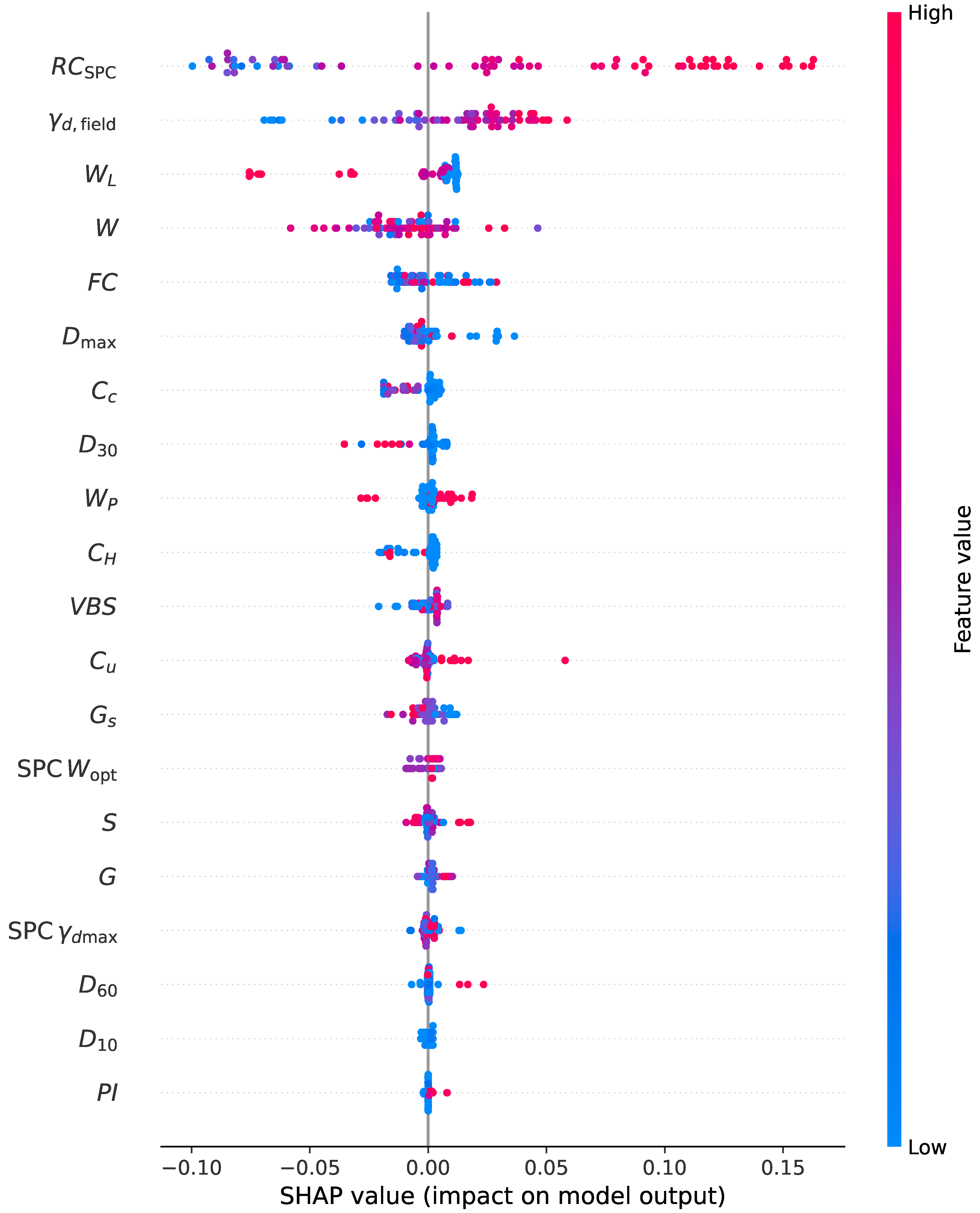
Model explanations were obtained with SHAP (SHapley Additive exPlanations), in which each prediction was decomposed into additive feature contributions derived from Shapley values in cooperative game theory [22,55,56,57]. In this setting, a global ranking of predictors is provided by the mean absolute SHAP value, and local directionality for each observation is given by the sign of the contribution. Summary beeswarm plots were produced for the XGBoost models of , , and (Figure 6, Figure 7 and Figure 8); each dot represents one sample, the horizontal axis shows the SHAP value, and the color encodes the raw feature value (blue = low, red = high). Throughout this subsection, explanations are understood as model-based associations conditional on the fitted algorithm and the empirical joint distribution of the predictors; they are not to be interpreted as causal effects. In addition, because several predictors were correlated (e.g., , , and W), the magnitude and sign of attributions were conditional and should be read as partial effects under collinearity. To mitigate over-interpretation, we triangulated SHAP with permutation importance, partial dependence (PDP), and accumulated local effects (ALEs).
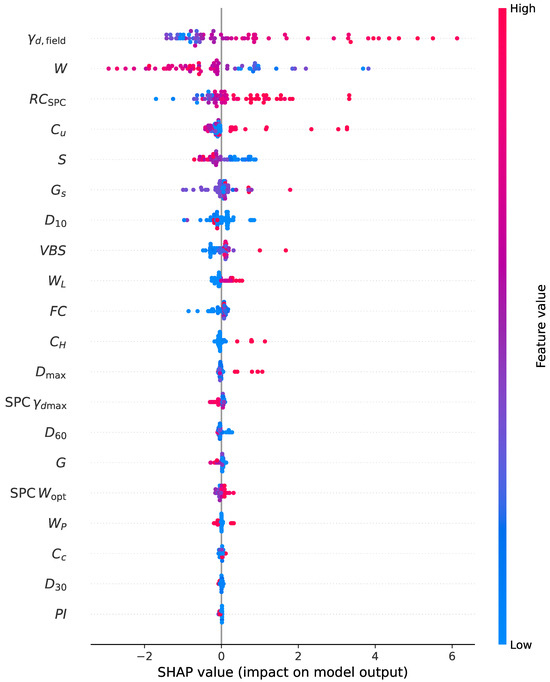
Figure 6.
SHAP beeswarm summary for the XGBoost model predicting qd0. Each dot represents one observation; the horizontal axis shows the SHAP value (feature contribution to the model output), and the color encodes the raw feature value (blue = low, red = high). Features are ordered by mean absolute SHAP.
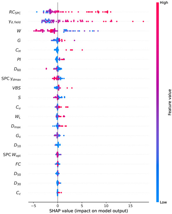
Figure 7.
SHAP beeswarm summary for the XGBoost model predicting qd1. Interpretation as in Figure 6.
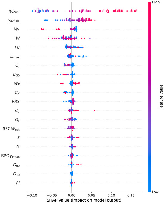
Figure 8.
SHAP beeswarm summary for the XGBoost model predicting Zc. Interpretation as in Figure 6.
A geotechnical reading of these summaries is provided to connect attributions with mechanisms. Variables tied to state (, W) and to compaction references (, ) were assigned the largest contributions across targets, while grain size and plasticity descriptors (for example, , FC, IP, and VBS) provided secondary adjustments. For (Figure 6), higher gd and larger were associated with positive SHAP values, which is consistent with higher dry density and a compaction state closer to the laboratory optimum yielding greater penetration resistance. Higher moisture was associated with negative contributions, in agreement with lubrication effects and loss of apparent suction away from the optimum water content. Color gradients along the horizontal axis suggested that the effect of moisture was not uniform over the range of and , indicating interaction between density state and W. Grain-size indicators with larger characteristic diameters (for example, ) tended to contribute positively, reflecting increased interlocking and stiffness in coarser fills; conversely, higher FC and higher plasticity (PI, VBS) tended to contribute negatively at comparable compaction states. These patterns align with established compaction mechanics, but they remain associational and conditional on correlated inputs; individual SHAP values should, therefore, not be construed as causal effects of the corresponding variables.
For qd1 (Figure 7), the same hierarchy was observed: and drove positive contributions and moisture drove negative contributions. The magnitude of moisture-related attributions appeared larger than for , which is compatible with the cumulative effect of pore water on the resistance after the initial seating. This pattern is consistent with the prediction–measurement comparison shown in Section 4.1, where underestimation at high values was noted, and it also suggests that departures from the optimal compaction water content are a plausible contributor to that bias in the upper tail. Again, these explanations are conditional on the trained model and the observed data distribution, and they should not be interpreted causally; correlated predictors may share or trade attribution mass.
For Zc (Figure 8), leading roles were assigned to gd and moisture, with and coarse-fraction indicators following. The dominance of density- and water-related variables across the three targets supports a coherent physical interpretation in which the state of compaction controls both the level of resistance and the depth-related response. Narrower spreads in SHAP values for were in line with the smaller inter-model differences observed in the scatter plots. The explanatory patterns for were likewise associational; they summarize how the fitted model organized the contributions under the observed correlations and do not imply causal mechanisms.
Two caveats are emphasized. First, SHAP values explain the behavior of the trained models rather than causal effects; signs and magnitudes are conditional on the remaining predictors and on the empirical joint distribution, as summarized in Figure 2. Second, several predictors were correlated by construction (for example, , , and W), so individual attributions should be read as conditional marginal effects. Consistent with these caveats, all interpretation is reported alongside permutation-based importance and effect-shape diagnostics (PDP and ALE) to provide convergent, non-causal evidence about influential predictors and their functional forms.
Beyond SHAP, complementary analyses were carried out with permutation importance, partial dependence plots (PDPs), and accumulated local effects (ALE). Permutation importance quantified the decrease in predictive accuracy after random shuffling of each variable, providing a robust global ranking (Figure 9).
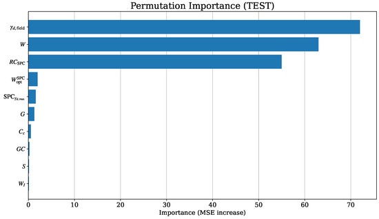
Figure 9.
Permutation importance on the test set (XGBoost for ). Bars report the increase in test MSE after permuting each feature; higher bars indicate more influential predictors.
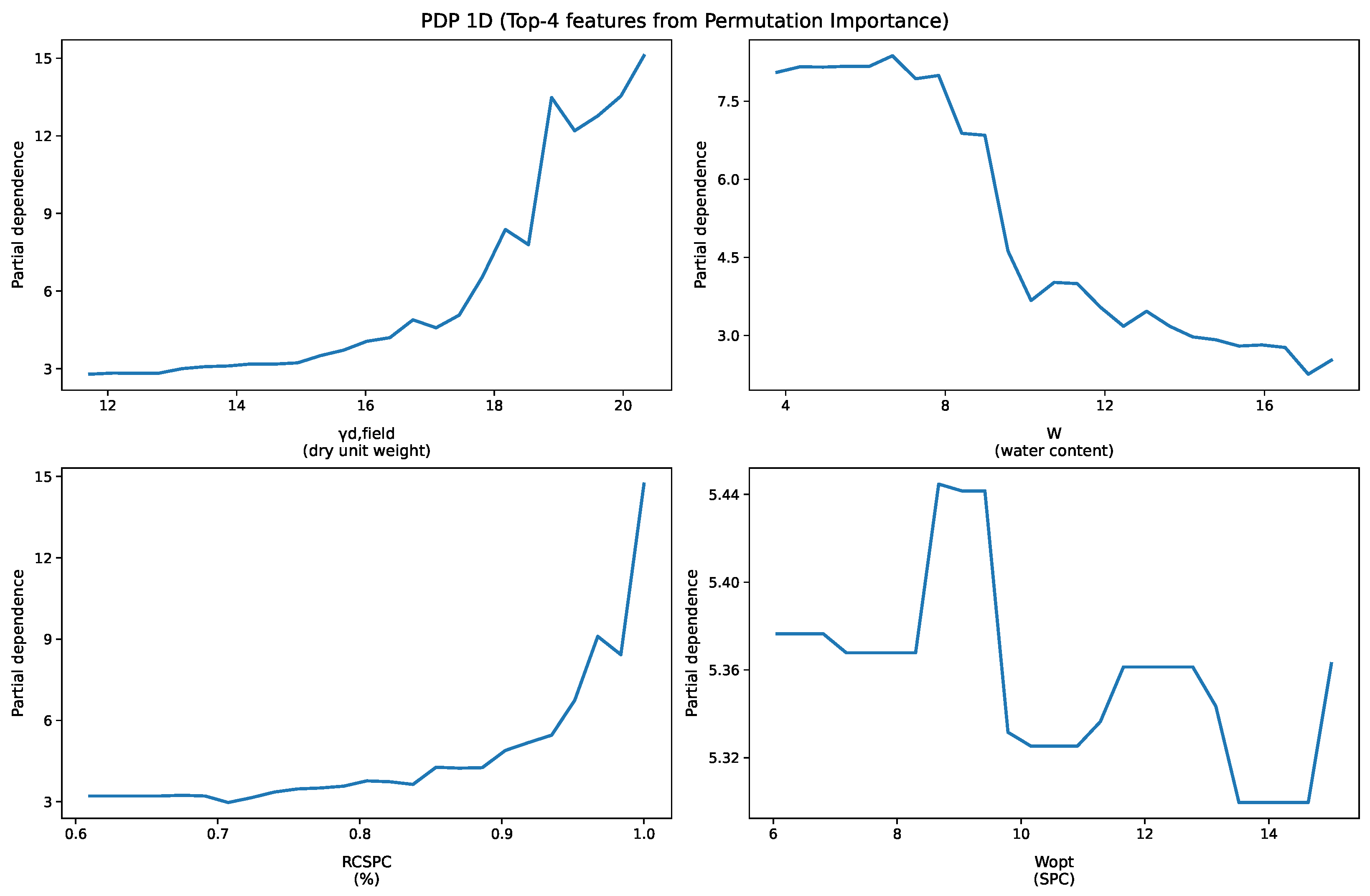
To interrogate the shape of the effects, 1D PDPs were produced for the four most influential predictors from permutation importance (Figure 10). A PDP shows the marginal effect of a feature on the model prediction while averaging over the distribution of the remaining inputs. The plots indicated the following: (i) a strongly increasing, non-linear response with , with a marked rise beyond ∼18 kN/m3; (ii) a monotonic increase with , especially near full compaction (0.95–1.00); (iii) a decreasing trend with water content W, with a knee around 9–10% consistent with departure from the optimal water condition; and (iv) a comparatively flat response with , suggesting that the observed variation in mainly acts through its relation with W and . The shapes and thresholds were coherent with the geotechnical mechanisms inferred from SHAP.
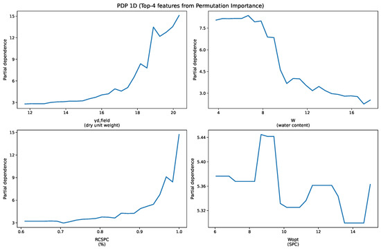
Figure 10.
The 1D partial dependence for the four most influential features (from permutation importance). Each panel shows the average model response as the selected feature varies over its observed range, averaging over the joint distribution of the remaining predictors.
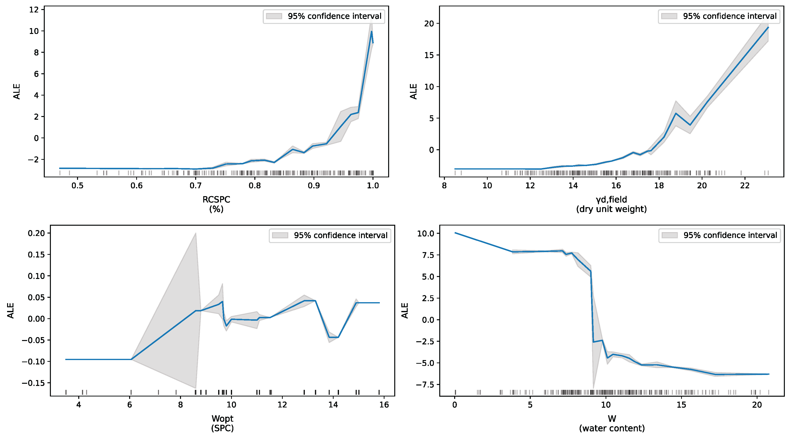
ALE plots were also generated (Figure 11). ALE is less sensitive to correlations among predictors and provides unbiased estimates of feature effects by local differencing. The ALE results confirmed the dominance of density- and water-related variables, with sharp increases in predicted response at high and , as well as a negative influence of increasing water content. The consistency between PDPs and ALE reinforces the physical interpretation that compaction state governs both the level of resistance and the progression of response.
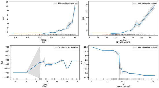
Figure 11.
The 1D accumulated local effects (ALEs) for the four most influential features. Shaded regions show 95% confidence intervals obtained by bootstrapping (PyALE default); tick marks on the x-axis indicate the empirical distribution.
For qd1 (Figure 7), the same hierarchy was observed: and drove positive contributions and moisture drove negative contributions. The magnitude of moisture-related attributions appeared larger than for , which is compatible with the cumulative effect of pore water on resistance after the initial seating. This pattern is consistent with the prediction–measurement comparison shown in Section 4.1, where underestimation was at a high values was noted, and findings suggest that departures from the optimal compaction water content are a plausible contributor to that bias in the upper tail.
For Zc (Figure 8), leading roles were assigned to gd and moisture, with and coarse-fraction indicators following. The dominance of density- and water-related variables across the three targets supports a coherent physical interpretation in which the state of compaction controls both the level of resistance and the depth-related response. Narrower spreads in SHAP values for were in line with the smaller inter-model differences observed in the scatter plots.
In the permutation importance analysis (Figure 9), the dry unit weight in the field () and the natural water content (W) emerged as the dominant predictors, followed by the compaction ratio (). These variables largely coincide with those highlighted by SHAP values, reinforcing the interpretation that soil density and moisture conditions primarily govern the predicted response. Minor contributions from grain size parameters indicate a secondary influence of texture on the model output.
To interrogate the shape of the effects, we produced 1D PDPs for the four most influential predictors from permutation importance (Figure 10). The plots indicate the following: (i) a strongly increasing, non-linear response with , with a marked rise beyond ∼18 kN/m3; (ii) a monotonic increase with , especially near full compaction (0.95–1.00); (iii) a decreasing trend with water content W, with a knee around 9–10% that is consistent with moving away from the optimal water condition; and (iv) a comparatively flat response with , suggesting that the observed variation in mainly acts through its relation with W and . The shapes and thresholds are coherent with the geotechnical mechanisms discussed with SHAP.
Because PDP averages can be biased under correlated predictors, we also constructed 1D ALE plots for the same four features (Figure 11). ALE confirms the main patterns: the effect of and was strongly positive and accelerated at the upper tail; the effect of W was negative after ∼9–10%; and the effect of was comparatively small. The narrow confidence ribbons for and indicate stable effects, whereas wider ribbons at the extremes of W reflect data sparsity. The convergence of SHAP, permutation importance, PDP, and ALE strengthens the conclusion that the compaction state (density and relative compaction) and the in situ water content control the predicted resistance.
4.4. Statistical Validation
This subsection reports a statistical assessment of the target variable predicted by all model families on the fixed 80/20 train–test split (random state 42). Uncertainty in test performance was quantified using bootstrap resamples of the test set. Pairwise model contrasts were performed with paired resampling that reused identical indices across models to ensure fair comparisons. Calibration was evaluated by regressing y on in the test set. Performance was summarized with , RMSE, and MAE. To minimize distributional assumptions, nonparametric bootstrap confidence intervals were reported, effect sizes accompanied p-values, and family-wise error across pairwise tests was controlled with Holm’s step-down adjustment [52,58,59,60,61]. A further limitation concerns data partitioning. Although the random split ensured representation of all GTR classes in both training and testing, it does not fully capture potential site effects. Future work should, therefore, examine grouped or site-wise validation with larger and more balanced datasets to evaluate cross-site generalization more explicitly.
The experimental design followed the fixed 80/20 train–test split defined in the pipeline. From the test set, bootstrap resamples were drawn by sampling rows with replacement. For each resample and model, , RMSE, and MAE were recomputed and percentile 95% confidence intervals were formed (Table 13). Model comparisons were performed with paired bootstrap tests on the RMSE using the same resampled indices for each pair, and we report (mean and 95% CI), two-sided p-values, and the effect sizes for paired designs (Cohen’s and Cliff’s ), with Holm-adjusted p-values to address multiplicity (Table 14). Calibration was evaluated by regressing y on in the test set and reporting the slope, intercept, and with bootstrap intervals; values near slope = 1 and intercept indicate good calibration (Table 15) [52].

Table 13.
Test metrics with 95% bootstrap CIs (B = 5000).

Table 14.
Paired bootstrap comparisons for all model pairs (RMSE). Holm-adjusted p-values.

Table 15.
Calibration of y vs. on the test set (slope/intercept/ with 95% CIs).
The test set estimates indicated that MLP achieved the lowest errors (, RMSE = 5.866, and MAE ), with XGB close behind (, RMSE ). RF and SVR showed lower and larger errors (Table 13). Paired bootstrap contrasts on the RMSE yielded the largest mean gap for SVR versus MLP (, 95% CI [0.385, 4.116]), yet no pairwise comparison remained significant after Holm adjustment (all adjusted ). For XGB versus MLP, with a confidence interval spanning zero and effect sizes were uniformly small; in particular, Cliff’s for XGB versus MLP denotes a negligible dominance effect (Table 14). Calibration on the test set was close to ideal for MLP and XGB (slopes 1.068 and 1.124; intercepts near zero; calibration and ), whereas SVR exhibited a larger slope (1.598), consistent with under-dispersion, and RF showed a milder version of this pattern (slope 1.246) (Table 15) [52].
In conclusion, considering bootstrap uncertainty, paired testing with effect sizes, and multiplicity control, the MLP provided the strongest overall performance on the hold out test set, with XGB a close second; their difference is not statistically significant at after Holm adjustment. Both MLP and XGB display favorable calibration, supporting their practical use for estimating , while RF and SVR serve as useful baselines with comparatively weaker accuracy and calibration. Future work should examine external-like validation via grouped or site-wise resampling, report prediction intervals derived from bootstrap resampling, and routinely monitor and update calibration upon deployment to new materials or sites [52,58,59].
5. Conclusions
This study examined whether supervised machine learning can provide accurate and interpretable surrogates of the LDCP indices , , and for compaction QA/QC. Using a curated multi-campaign dataset () that couples LDCP results with routine geotechnical descriptors, we implemented a single pipeline across linear (ridge/lasso/elastic net); kernel (SVR); tree-ensemble (Random Forest, XGBoost); and neural (MLP) learners.
For , the MLP achieved the lowest test error (, RMSE ), and XGBoost was close behind (, RMSE ). Importantly, paired bootstrap testing with Holm adjustment showed that the MLP–XGBoost gap was not statistically significant, indicating that both models can be regarded as equally effective on this dataset. Calibration slopes were near unity for both models, supporting practical use. The naïve GTR-average baseline performed poorly, underscoring the added value of incorporating state and material descriptors.
Interpretability analyses (SHAP, permutation importance, PDP, ALEs) were mutually consistent and aligned with soil-mechanics expectations: density/state and moisture (, , W) dominated the response, while gradation and plasticity provided secondary adjustments. These explanations are inherently model-based and conditional on correlated predictors; they should not be interpreted as causal effects.
To connect predictions to field decision making, we reported split-conformal prediction intervals and a simple three-way QA/QC rule: accept if the lower bound exceeds the threshold T, reject if the upper bound is below T, and classify as a gray zone otherwise. This procedure offers transparent, finite-sample coverage guarantees under exchangeability, and it enables explicit control of false acceptance/rejection rates.
Limitations include the moderate sample size and the use of a fixed random 80/20 split, which—while preserving GTR coverage and reducing leakage across independent observations—does not fully isolate potential site effects. Several predictors were correlated by construction (e.g., , , and W), so individual attributions are conditional. A slight underestimation in the upper tail of suggests sensitivity to departures from . Computation was not a constraint (sub-second inference; s training per model on CPU).
Future work should prioritize external-like assessment via grouped or site-wise resampling once classes overlap across sites; explore truncated-input configurations for deployments where some descriptors may be unavailable; incorporate physically informed constraints (e.g., monotonicity in and W); extend to multi-task learning for joint / prediction; integrate with intelligent compaction to fuse ICMVs and model outputs for closed-loop control; and advance cross-device/energy-transfer standardization to support broader adoption. Finally, routine calibration monitoring and interval reporting (e.g., bootstrap or conformal) are recommended for deployment.
Author Contributions
Conceptualization, J.R.-V. and J.G. (José García); methodology, J.R.-V. and J.G. (José García); software, J.R.-V.; validation, G.V. (Gabriel Villavicencio), M.B., A.H., P.B., G.V. (German Varas), P.M., J.G. (Jose Gornall), and H.P.; formal analysis, J.R.-V. and J.G. (José García); investigation, J.R.-V. and J.G. (José García); data curation, J.R.-V. and J.G. (José García); writing—original draft preparation, J.R.-V. and J.G. (José García); writing—review and editing, G.V. (Gabriel Villavicencio), M.B., A.H., P.B., G.V. (German Varas), P.M., J.G. (Jose Gornall), and H.P.; visualization, J.R.-V.; supervision, H.P. and P.B.; project administration, J.R.-V. and H.P. All authors have read and agreed to the published version of the manuscript.
Funding
This research was funded by FONDEF ANID, grant ID23I10249, project Sand Guardian.
Data Availability Statement
The data presented in this study are available on request from the corresponding authors. (The data are based on real laboratory tests, and confidentiality agreements prevent open sharing).
Conflicts of Interest
The authors declare no conflicts of interest.
References
- ASTM D698-12; Standard Test Methods for Laboratory Compaction Characteristics of Soil Using Standard Effort (12,400 ft·lbf/ft3 (600 kN·m/m3)). ASTM International: West Conshohocken, PA, USA, 2021. [CrossRef]
- ASTM D1557; Test Methods for Laboratory Compaction Characteristics of Soil Using Modified Effort (56,000 ft·lbf/ft3 (2,700 kN·m/m3)). ASTM International: West Conshohocken, PA, USA, 2021. [CrossRef]
- EN 13286-2:2010; and Hydraulically Bound Mixtures—Part 2: Test Methods for Laboratory Reference Density and Water Content—Proctor Compaction. CEN: Brussels, Belgium, 2010.
- ASTM D1556; Test Method for Density and Unit Weight of Soil in Place by Sand-Cone Method. ASTM International: West Conshohocken, PA, USA, 2024. [CrossRef]
- ASTM D6938; Test Methods for In-Place Density and Water Content of Soil and Soil–Aggregate by Nuclear Methods (Shallow Depth). ASTM International: West Conshohocken, PA, USA, 2023. [CrossRef]
- ASTM D6951; Test Method for Use of the Dynamic Cone Penetrometer in Shallow Pavement Applications. ASTM International: West Conshohocken, PA, USA, 2018. [CrossRef]
- ASTM E2583; Test Method for Measuring Deflections with a Light Weight Deflectometer (LWD). ASTM International: West Conshohocken, PA, USA, 2020. [CrossRef]
- ASTM E2835; Test Method for Measuring Deflections Using a Portable Impulse Plate Load Test Device. ASTM International: West Conshohocken, PA, USA, 2021. [CrossRef]
- Soil—Testing Procedures and Testing Equipment—Plate Load Test; DIN/Beuth Verlag: Berlin, Germany, 2012; (English translation available).
- Geotechnical Investigation and Testing—Field Testing—Part 2: Dynamic Probing; ISO: Geneva, Switzerland, 2005.
- Lee, C.; Kim, K.S.; Woo, W.; Lee, W. Soil Stiffness Gauge (SSG) and Dynamic Cone Penetrometer (DCP) tests for estimating engineering properties of weathered sandy soils in Korea. Eng. Geol. 2014, 169, 91–99. [Google Scholar] [CrossRef]
- Kim, S.Y.; Lee, J.S.; Park, G.; Hong, W.T. Evaluation of Dynamic Resistance for Application of Portable In-Situ Device to Extra Target Depth. KSCE J. Civ. Eng. 2022, 26, 4195–4201. [Google Scholar] [CrossRef]
- Sun, H.; Xu, Q.; Sun, D.A.; Zhu, X. Energy-based comparison between a dynamic cone penetrometer and a motor-operated static cone penetrometer. Soil Tillage Res. 2011, 113, 124–133. [Google Scholar] [CrossRef]
- Farshbaf Aghajani, H.; Hatefi Diznab, M. A statistical investigation of dynamic cone penetrometer test. Int. J. Geosynth. Ground Eng. 2023, 9, 8. [Google Scholar] [CrossRef]
- Ahmad, M.; Al-Zubi, M.A.; Kubińska-Jabcoń, E.; Majdi, A.; Al-Mansob, R.A.; Sabri, M.M.S.; Ali, E.; Naji, J.A.; Elnaggar, A.Y.; Zamin, B. Predicting California bearing ratio of HARHA-treated expansive soils using Gaussian process regression. Sci. Rep. 2023, 13, 13593. [Google Scholar] [CrossRef]
- Almuaythir, S.; Zaini, M.S.I.; Lodhi, R.H. Predicting soil compaction parameters in expansive soils using advanced machine learning models: A comparative study. Sci. Rep. 2025, 15, 24018. [Google Scholar] [CrossRef]
- Kardani, N.; Aminpour, M.; Raja, M.N.A.; Kumar, G.; Bardhan, A.; Nazem, M. Prediction of the resilient modulus of compacted subgrade soils using ensemble machine learning methods. Transp. Geotech. 2022, 36, 100827. [Google Scholar] [CrossRef]
- Hu, X.; Solanki, P. Predicting Resilient Modulus of Cementitiously Stabilized Subgrade Soils Using Neural Network, Support Vector Machine, and Gaussian Process Regression. Int. J. Geomech. 2021, 21, 04021073. [Google Scholar] [CrossRef]
- Almuaythir, S.; Zaini, M.S.I.; Hasan, M.; Hoque, M.I. Stabilization of expansive clay soil using shells based agricultural waste ash. Sci. Rep. 2025, 15, 10186. [Google Scholar] [CrossRef]
- Almuaythir, S.; Abbas, M.F. Expansive soil remediation using cement kiln dust as stabilizer. Case Stud. Constr. Mater. 2023, 18, e01983. [Google Scholar] [CrossRef]
- Park, G.; Kim, N.; Kang, S.; Kim, S.Y.; Yoo, C.; Lee, J.S. Instrumented dynamic cone penetrometer incorporated with time domain reflectometry. Measurement 2023, 206, 112337. [Google Scholar] [CrossRef]
- Lundberg, S.M.; Lee, S.I. A Unified Approach to Interpreting Model Predictions. In Proceedings of the Advances in Neural Information Processing Systems 30 (NeurIPS 2017), Long Beach, CA, USA, 4–9 December 2017. [Google Scholar]
- Ngo, A.Q.; Nguyen, L.Q.; Tran, V.Q. Developing interpretable machine learning–Shapley additive explanations model for unconfined compressive strength of cohesive soils stabilized with geopolymer. PLoS ONE 2023, 18, e0286950. [Google Scholar] [CrossRef]
- Bozorgzadeh, E.; Feng, Y.J. Evaluation structures for machine learning models in geotechnical engineering: Problem, data, and algorithm. Georisk Assess. Manag. Risk Eng. Syst. Geohazards 2024, 18, 60–76. [Google Scholar] [CrossRef]
- Das, B.M. Principles of Geotechnical Engineering, 9th ed.; Cengage Learning: Boston, MA, USA, 2016. [Google Scholar]
- Lambe, T.W.; Whitman, R.V. Soil Mechanics; Wiley: New York, NY, USA, 1979. [Google Scholar]
- Seed, H.B.; Chan, C.K. Structure and strength characteristics of compacted clays. J. Soil Mech. Found. Div. ASCE 1959, 85, 87–128. [Google Scholar] [CrossRef]
- AASHTO. AASHTO Guide for Design of Pavement Structures; American Association of State Highway and Transportation Officials: Washington, DC, USA, 2017. [Google Scholar]
- Alonso, E.E.; Gens, A. Aznalcóllar dam failure. Part 1: Field observations and material properties. Géotechnique 2006, 56, 165–183. [Google Scholar] [CrossRef]
- Federal Highway Administration. Utilizing Intelligent Compaction to Ensure Quality and Uniformity of Pavement Foundation; Technical Report FHWA-HIF-24-097; Tech Brief; U.S. Department of Transportation, FHWA: McLean, VA, USA, 2024.
- Zhang, Q.; An, Z.; Huangfu, Z.; Li, Q. A Review on Roller Compaction Quality Control and Assurance Methods for Earthwork in Five Application Scenarios. Materials 2022, 15, 2610. [Google Scholar] [CrossRef]
- T 99-21; Moisture–Density Relations of Soils Using a 2.5-kg (5.5-lb) Rammer and a 305-mm (12-in.) Drop. AASHTO: Washington, DC, USA, 2021.
- T 180-22; Moisture–Density Relations of Soils Using a 4.54-kg (10-lb) Rammer and a 457-mm (18-in.) Drop. AASHTO: Washington, DC, USA, 2022.
- Baek, S.H.; Cho, J.W.; Kim, J.Y. Field study on intelligent compaction for compaction quality control of subgrade bases. Can. Geotech. J. 2025, 62, 1–14. [Google Scholar] [CrossRef]
- Gourvès, R.; Barjot, R. Le Pénétromètre Dynamique Léger PANDA, The PANDA Ultralight Dynamic Penetrometer. In Proceedings of the Eleventh European Conference on Soil Mechanics and Foundation Engineering, Copenhagen, Denmark, 28 May–1 June 1995. [Google Scholar]
- Benz-Navarrete, M.A.; Breul, P.; Bacconnet, C.; Moustan, P. The PANDA®, Variable Energy Lightweight Dynamic Cone Penetrometer: A quick state of art. ASTM J. 2020. Available online: https://api.semanticscholar.org/CorpusID:232155737 (accessed on 1 September 2025).
- Rojas-Vivanco, J.; Barbier, S.; Navarrete, M.A.B.; Breul, P. Statistical Analysis of the Influence of Ballast Fouling on Penetrometer and Geoendoscope Data. Adv. Transp. Geotech. IV 2021, 165, 915–930. [Google Scholar] [CrossRef]
- NF P94-105; Sols: Reconnaissance et essais—Contrôle de la qualité du compactage—Méthode au pénétromètre dynamique à énergie variable—Principe et méthode d’étalonnage du pénétromètre—Exploitation des résultats—Interprétation. AFNOR: Paris, France, 2000.
- Herath, A.; Mohammad, L.N.; Gaspard, K.; Gudishala, R.; Abu-Farsakh, M.Y. The Use of Dynamic Cone Penetrometer to Predict Resilient Modulus of Subgrade Soils. In Proceedings of the Advances in Pavement Engineering, GeoFrontiers 2005, Reston, VA, USA, 24–26 January 2005; pp. 313–322. [Google Scholar] [CrossRef]
- Mousavi, S.H.; Gabr, M.A.; Borden, R.H. Resilient modulus prediction of soft low-plasticity Piedmont residual soil using dynamic cone penetrometer. J. Rock Mech. Geotech. Eng. 2018, 10, 323–332. [Google Scholar] [CrossRef]
- Keskin, İ.; Memiş, M.A. Prediction of soil strength and dynamic properties through the dynamic cone penetration index. Discov. Civ. Eng. 2025, 2, 142. [Google Scholar] [CrossRef]
- ASTM D7380-08; Standard Test Method for Soil Compaction Determination at Shallow Depths Using 5-lb (2.3-kg) Dynamic Cone Penetrometer. ASTM International: West Conshohocken, PA, USA, 2008. [CrossRef]
- IS 2131-1981; Method for Standard Penetration Test for Soils. Bureau of Indian Standards: New Delhi, India, 1981.
- IS 4968; (Part 2); Method for Subsurface Sounding for Soils: Dynamic Method Using Cone and Bentonite Slurry. Bureau of Indian Standards: New Delhi, India, 1976.
- Chen, C.; Shen, S.; Arulrajah, A.; Wu, H. Correlations between dynamic cone penetration test results and soil properties: A review. Soils Found. 2018, 58, 425–450. [Google Scholar] [CrossRef]
- George, R.M.D.; Rao, K.V.R.; Shivashankar, R. PFWD, DCP and CBR correlations for evaluation of lateritic subgrades. Int. J. Pavement Eng. 2009, 10, 189–199. [Google Scholar] [CrossRef]
- Mohammadi, S.D.; Nikoudel, M.R.; Rahimi, H.; Khamehchiyan, M. Application of the Dynamic Cone Penetrometer (DCP) for determination of the engineering parameters of sandy soils. Eng. Geol. 2008, 101, 195–203. [Google Scholar] [CrossRef]
- Ampadu, S.I.K.; Fiadjoe, P. Influence of water content on the dynamic cone penetration index and the California Bearing Ratio of a lateritic subbase. Transp. Geotech. 2015, 5, 68–85. [Google Scholar] [CrossRef]
- Jas, K.; Dodagoudar, G.R. Explainable machine learning model for liquefaction potential assessment of soils using XGBoost–SHAP. Soil Dyn. Earthq. Eng. 2023, 165, 107662. [Google Scholar] [CrossRef]
- SETRA–LCPC. GTR Guide des Terrassements Routiers: Réalisation des Remblais et des Couches de Forme; SETRA–LCPC: Paris-Bagneux, France, 1992; Available online: https://doc.cerema.fr/Default/doc/SYRACUSE/14456/realisation-des-remblais-et-des-couches-de-forme-GTR-Fascicule-1-et-2.pdf (accessed on 1 September 2025).
- D2487-17; Standard Practice for Classification of Soils for Engineering Purposes (Unified Soil Classification System). ASTM International: West Conshohocken, PA, USA, 2017.
- Calster, B.V.; McLernon, D.J.; van Smeden, M.; Wynants, L.; Steyerberg, E.W. Calibration: The Achilles Heel of Predictive Analytics. BMC Med. 2019, 17, 230. [Google Scholar] [CrossRef]
- Lei, J.; G’Sell, M.; Rinaldo, A.; Tibshirani, R.J.; Wasserman, L. Distribution-free predictive inference for regression. J. Am. Stat. Assoc. 2018, 113, 1094–1111. [Google Scholar] [CrossRef]
- Angelopoulos, A.N.; Bates, S. A gentle introduction to conformal prediction and distribution-free uncertainty quantification. arXiv 2021, arXiv:2107.07511. [Google Scholar]
- Shapley, L.S. A Value for n-Person Games. In Contributions to the Theory of Games; Annals of Mathematics Studies; Kuhn, H.W., Tucker, A.W., Eds.; Princeton University Press: Princeton, NJ, USA, 1953; Volume 28, pp. 307–317. [Google Scholar] [CrossRef]
- Lundberg, S.M.; Erion, G.; Chen, H.; DeGrave, A.; Prutkin, J.M.; Nair, B.; Katz, R.; Himmelfarb, J.; Bansal, N.; Lee, S.I. From local explanations to global understanding with explainable AI for trees. Nat. Mach. Intell. 2020, 2, 56–67. [Google Scholar] [CrossRef] [PubMed]
- Lundberg, S.M.; Erion, G.G.; Lee, S.I. Consistent individualized feature attribution for tree ensembles. arXiv 2018, arXiv:1802.03888. [Google Scholar]
- Efron, B.; Tibshirani, R.J. An Introduction to the Bootstrap; Chapman & Hall/CRC: New York, NY, USA, 1993. [Google Scholar] [CrossRef]
- Holm, S. A Simple Sequentially Rejective Multiple Test Procedure. Scand. J. Stat. 1979, 6, 65–70. [Google Scholar]
- Lakens, D. Calculating and Reporting Effect Sizes to Facilitate Cumulative Science: A Practical Primer for t-Tests and ANOVAs. Front. Psychol. 2013, 4, 863. [Google Scholar] [CrossRef] [PubMed]
- Meissel, K.; Yao, E.S. Using Cliff’s Delta as a Non-Parametric Effect Size Measure: An Accessible Web App and R Tutorial. Pract. Assess. Res. Eval. 2024, 29, 2. [Google Scholar] [CrossRef]
Disclaimer/Publisher’s Note: The statements, opinions and data contained in all publications are solely those of the individual author(s) and contributor(s) and not of MDPI and/or the editor(s). MDPI and/or the editor(s) disclaim responsibility for any injury to people or property resulting from any ideas, methods, instructions or products referred to in the content. |
© 2025 by the authors. Licensee MDPI, Basel, Switzerland. This article is an open access article distributed under the terms and conditions of the Creative Commons Attribution (CC BY) license (https://creativecommons.org/licenses/by/4.0/).

