Upper and Lower Bounds of Performance Metrics in Hybrid Systems with Setup Time

Abstract

To address the increasing demand for computational and communication resources, modern networked systems often rely on heterogeneous servers, including those requiring setup times, such as virtual machines or servers, and others that are always active. In this paper, we model and analyze the performance of such hybrid systems using a level-dependent quasi-birth-and-death (LDQBD) process. Building upon an existing queueing model, we extend the analysis by considering scalable approximation methods. Since matrix analytic methods become computationally expensive in large-scale settings, we propose a stochastic bounding approach that derives upper and lower bounds for the stationary distribution, thereby significantly reducing computational cost. This approach further provides bounds on the performance metrics of the hybrid system.

1. Introduction

In recent years, communication traffic has been steadily increasing, driven by factors such as the widespread use of Internet-connected devices, including smartphones and tablets, and the growing volume of data generated by digital transformation (DX). To meet this rising demand, 5G networks have been widely deployed. While 5G networks offer high capacity, high speed, low latency, and massive connectivity, they also raise concerns about increased power consumption. As a result, developing operational strategies to mitigate energy-related costs has become a crucial research challenge.

In mobile networks, many network functions are now virtualized, resulting in configurations that combine legacy network equipment with virtualized network functions, resembling a non-standalone 5G architecture. Legacy equipment remains continuously powered on, whereas virtual network functions (VNFs) can be dynamically activated or deactivated. In order to design such a hybrid system that minimizes power consumption, it is important to conduct performance analysis based on mathematical modeling.

A study closely related to the present work is that of Sato et al. [1], who modeled a hybrid system consisting of both servers running on legacy network equipment (hereafter referred to as legacy servers) and virtualized servers (hereafter referred to as virtual servers) that require setup time to become active. Their model extends the frameworks proposed by Phung-Duc et al. [2] and Ren et al. [3] to allow for different processing rates between legacy and virtual servers. Importantly, their model assumes that once a job is assigned to a virtual server, it cannot be transferred back to a legacy server. For details of the job assignment policy, see Sato et al. [1]. They formulated the system as a level-dependent quasi-birth-and-death (LDQBD) process and analyzed its stationary behavior.

In contrast to the models in Phung-Duc et al. [2] and Ren et al. [3], where the special transition structure of the LDQBD process allows efficient computation of stationary performance metrics using the technique of Phung-Duc and Kawanishi [4], the model in Sato et al. [1] lacks such a structure. Consequently, their stationary analysis relies on standard matrix analytic methods.

For the matrix analytic methods, see, for example, Neuts [5] and Latouche and Ramaswami [6]. See also Artalejo and Gómez-Corral [7] for a recent study on queueing systems with complex dynamics. Algorithms for computing the stationary distribution of LDQBD processes were proposed by Bright and Taylor [8], Phung-Duc et al. [9], Baumann and Sandmann [10]. For more general Markov processes, including LDQBD processes, a sequential update algorithm was developed by Masuyama [11]. Since matrix analytic methods require matrix operations, they might become computationally intensive and thus impractical for large-scale systems, as the computational cost grows significantly with the system size (e.g., the number of virtual servers) due to the large matrix dimensions involved.

To address this issue, we focus on bounds for the stationary distribution and its expectations. There is a substantial body of literature analyzing bounds on stationary expectations for Markov processes, including LDQBD processes. Bounding the stationary distribution and performance metrics with the help of a Lyapunov function [12,13] is a common technique in the literature on stochastic models and their applications. For example, systems of stochastic chemical kinetics have been analyzed using LDQBD processes [14], where the Lyapunov function-based approach was applied to bound their stationary distribution. By leveraging information about the moments of the state variables of a Markov process, together with the Lyapunov function-based approach, a tight bounding technique was proposed in [15].

Another approach to obtaining bounds for the stationary distribution is to utilize stochastic comparison methods (see, e.g., [16,17]). The key idea of this approach is to design a new Markov process whose stationary distribution serves as an upper or lower bound, in a certain stochastic ordering, for the stationary distribution of the original Markov process. For an algorithmic approach to such stochastic bounds, see [18]. Furthermore, structural properties of Markov processes, such as lumpability [19] and censoring [20], have also been exploited in bounding techniques [21,22].

In this paper, we analyze the same system model as in Sato et al. [1], which involves both servers with and without setup times formulated as an LDQBD process. Since matrix analytic methods become computationally expensive in large-scale settings, we apply the bounding technique developed by Bright and Taylor [8] to this model. By exploiting the transition structure of the model, we derive upper and lower stochastic bounds for the stationary distribution, which can be computed via recurrence relations without resorting to matrix-based operations. This approach leads to a significant reduction in computational cost. Our contributions are threefold.

• We refine the upper bounding model developed by Bright and Taylor [8], making it tighter across a wider range of system parameters.
• We derive recurrence relations for the stationary distribution that avoid matrix-analytic computations, thereby improving computational efficiency. This development relies on specific structural properties of the transition rates, as in Sato et al. [1].
• We extend the analysis of Kawanishi [23] and further develop a stochastic lower bounding model within the same framework.

We further show that key performance metrics, such as the expected sojourn time computed from the true stationary distribution, are bounded above and below by our proposed stochastic bounds. In addition, we conduct numerical experiments to evaluate the sensitivity of these performance metrics to variations in system parameters.

The remainder of this paper is organized as follows. Section 2 describes the system model. Section 3 provides a brief overview of partial order relations and stochastic dominance. Section 4 and Section 5 introduce the proposed upper and lower bounding models, respectively. Section 6 discusses performance bounds based on the proposed upper and lower bounding models. Section 7 presents numerical examples to validate the proposed approach. Finally, Section 8 concludes this paper.

2. System Model

We consider a queueing system with multiple servers, consisting of both legacy servers and virtual servers. Legacy servers are assumed to be always powered on, and incoming jobs are assigned to them preferentially in order to reduce power consumption. When all legacy servers are busy, jobs are assigned to virtual servers. Virtual servers require a setup time before they become available to process jobs. Once a job is assigned to a server, either legacy or virtual, it is completed on that server without migration. After completing a job, a virtual server is immediately turned off if no jobs are waiting in the queue.

Jobs are processed in the order of arrival, i.e., according to the first-come, first-served discipline. If servers are available and no jobs are waiting, an arriving job is processed immediately. Otherwise, the job enters a finite-capacity waiting room. If the buffer is full on arrival, the job is rejected and lost. Each waiting job is associated with a deadline by which its service must begin. If the job’s service is not started before its deadline, it leaves the system without being processed.

Let l and v denote the number of legacy servers and virtual servers, respectively, so that the total number of servers is l + v. The maximum capacity of the entire queueing system, including both servers and waiting space, is denoted by K, and we assume K ≥ l + v. Jobs arrive at the system according to a Poisson process with rate λ. The deadline time associated with each job is assumed to follow an exponential distribution with mean 1 / θ. Service times are exponentially distributed. The mean service time is 1 / μ for legacy servers and 1 / μ_v for virtual servers. The setup time required before a virtual server becomes active is also assumed to be exponentially distributed, with mean 1 / α. The parameters of the queueing system are summarized in Table 1.

Table 1. Parameters of queueing system.

Parameter	Description
l	Number of legacy servers
v	Number of virtual servers
K	Maximum capacity of the entire queueing system
λ	Arrival rate of jobs
θ	Deadline expiry rate of waiting jobs
μ	Service rate of legacy servers
μv	Service rate of virtual servers
α	Setup rate of virtual servers

Based on the conditions described above, we model the system as a two-dimensional continuous-time Markov chain $\{X(t)=(N(t),J(t));t\ge 0\}$, where N(t) denotes the number of active virtual servers that have completed setup at time t, and J(t) represents the total number of jobs being processed by legacy servers and those waiting in the queue at time t. The state space S of the Markov chain $\{X(t)=(N(t),J(t));t\ge 0\}$ is defined as

$$\begin{array}{c}\hfill S=\{(i,j)\mid 0\le i\le v,0\le j\le K-i\}.\end{array}$$

The continuous-time Markov chain $\{X(t)=(N(t),J(t));t\ge 0\}$ can be regarded as a finite LDQBD process, where J(t) represents the level and N(t) the phase. The transition rate matrix Q of this LDQBD process has the following block-tridiagonal structure:

$$\begin{array}{cc}\hfill Q& =\left[\begin{array}{ccccc}{Q}_1^{(0)}& Q_0^{(0)}& O& \dots & O\\ Q_2^{(1)}& Q_1^{(1)}& Q_0^{(1)}& \ddots & ⋮\\ O& Q_2^{(2)}& Q_1^{(2)}& \ddots & O\\ ⋮& \ddots & \ddots & \ddots & Q_0^{(K-1)}\\ O& \dots & O& Q_2^{(K)}& Q_1^{(K)}\end{array}\right],\hfill \end{array}$$

where the block matrices $Q_0^{(j)}$ (for 0 ≤ j ≤ K − 1), $Q_1^{(j)}$ (for 0 ≤ j ≤ K), and $Q_2^{(j)}$ (for 1 ≤ j ≤ K) represent the transitions that increase, preserve, and decrease the level, respectively. The explicit forms of these block matrices are provided in Appendix A. As an illustrative example, Figure 1 shows the state transition diagram for the case where l = 2, v = 2, and K = 5.

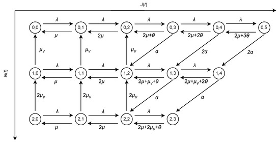
Figure 1. State transition diagram of the model on the state space S.

We can confirm that the generator matrix Q is irreducible. Since the state space is finite, the LDQBD process has a unique stationary distribution π, which satisfies the following system of linear equations

$$\begin{array}{cc}\hfill \mathit{\pi }Q& =\mathbf{0},\mathit{\pi }\mathbf{1}=1,\hfill \end{array}$$

where 0 is the row vector of all zeros, and 1 is the column vector of all ones. Thanks to the block tridiagonal structure of Q, it is well known that π can be computed using the matrix analytic method [6]. Specifically, if we partition the stationary distribution as π = (π₀, π₁, …, π_K), where

$$\begin{array}{cc}\hfill {\mathit{\pi }}_j& =({\pi }_{0,j},{\pi }_{1,j},\dots ,{\pi }_{min\{K-j,v\},j}),0\le j\le K,\hfill \end{array}$$

and

$$\begin{array}{cc}\hfill {\pi }_{i,j}& =\underset{t\to \infty }{lim}Pr(X(t)=(i,j)),(i,j)\in S,\hfill \end{array}$$

then the vectors π_j can be computed recursively as

$$\begin{array}{cc}\hfill {\mathit{\pi }}_j& ={\mathit{\pi }}_{j-1}{R}^{(j)},j=1,2,\dots ,K,\hfill \end{array}$$

where the rate matrix R^(j) is defined by

$$\begin{array}{cc}\hfill R^{(j)}& =Q_0^{(j-1)}{(-U^{(j)})}^{-1},j=1,2,\dots ,K,\hfill \end{array}$$

and the auxiliary matrices U^(j) are computed via the backward recursion

$$\begin{array}{cc}\hfill U^{(K)}& =Q_1^{(K)},U^{(j)}=Q_1^{(j)}+Q_0^{(j)}{(-U^{(j+1)})}^{-1}{Q}_2^{(j+1)},j=0,1,\dots ,K-1.\hfill \end{array}$$

The vector π₀ is obtained as the solution to ${\mathit{\pi }}_0{U}^{(0)}=\mathbf{0}$. The normalization condition $\mathit{\pi }\mathbf{1}=1$ leads to

$$\begin{array}{c}\hfill {\mathit{\pi }}_0\mathbf{1}+{\mathit{\pi }}_0{R}^{(1)}\mathbf{1}+{\mathit{\pi }}_0{R}^{(1)}{R}^{(2)}\mathbf{1}+\dots +{\mathit{\pi }}_0{R}^{(1)}{R}^{(2)}\dots R^{(K)}\mathbf{1}=1.\end{array}$$

As the size of the block matrices increases, the computational cost grows significantly, especially for large-scale systems. It can be verified that the total number of states of the model is

$$\begin{array}{c}\hfill (v+1)(K+1-v)+{\displaystyle \frac{v(v+1)}{2}}=(v+1)(l+\mathsf{\Delta }+1)+{\displaystyle \frac{v(v+1)}{2}},\end{array}$$

where Δ = K − v − l ≥ 0. To obtain the stationary distribution of all states, it is necessary to compute R^(j) for 1 ≤ j ≤ K. In what follows, we focus on R^(j) for 1 ≤ j ≤ K and treat v as an input parameter to analyze the computational complexity with respect to v. Specifically, the size of R^(j) for 1 ≤ j ≤ K is

$$\begin{array}{c}\hfill (min\{K-j+1,v\}+1)\times (min\{K-j,v\}+1).\end{array}$$

Hence, there are K − v = l + Δ matrices of size (v + 1) × (v + 1), and one matrix of size (k + 1) × k for each 1 ≤ k ≤ v. The total space required to store R^(j) for 1 ≤ j ≤ K is therefore

$$\begin{array}{c}\hfill {(v+1)}^2(K-v)+\sum _{k=1}^v(k+1)k={(v+1)}^2(l+\mathsf{\Delta })+{\displaystyle \frac{v(v+1)(v+2)}{3}}.\end{array}$$

Thus, the space complexity grows as O(v³) with v. Since the most computationally expensive operations for evaluating R^(j) are matrix multiplications, it can be verified that the total time required to obtain R^(j) for 1 ≤ j ≤ K is

$$\begin{array}{c}\hfill {(v+1)}^3\times (K-v)+\sum _{k=1}^{v}k\times (k+1)k,\end{array}$$

which is of the order O(v⁴).

To reduce the computational cost of obtaining the stationary distribution, it is effective to adopt the recurrence-based method proposed in Phung-Duc and Kawanishi [4]. However, the transition structure of the model considered in this paper differs from that of the model in Phung-Duc and Kawanishi [4], which prevents direct application of their recurrence-based approach. To address this issue, we construct LDQBD processes that stochastically dominate the original process { X(t) = (N(t), J(t)); t ≥ 0 }, and whose stationary distributions can be computed via recurrence relations.

3. Partial Order Relation and Stochastic Dominance on S

3.1. Partial Order on S

Following the framework of Bright and Taylor [8], we introduce a partial order ⪯ on the state space S defined in Section 2. The quasi order ≺ and the associated partial order ⪯ are defined as follows.

Definition 1

(Quasi order). For two states $(i_1,j_1)\in S$ and $(i_2,j_2)\in S$, we write $(i_1,j_1)\prec (i_2,j_2)$ if

$$\begin{array}{c}\hfill j_1<j_2.\end{array}$$

Definition 2

(Partial order). For $(i_1,j_1),(i_2,j_2)\in S$, we write $(i_1,j_1)⪯(i_2,j_2)$ if

$$\begin{array}{c}\hfill (i_1,j_1)=(i_2,j_2) \mathit{or} (i_1,j_1)\prec (i_2,j_2).\end{array}$$

This ordering will be used in the next subsection to establish stochastic dominance between the original LDQBD process and its bounding processes; see Bright and Taylor [8] for further background.

3.2. Stochastic Dominance on S

We now define stochastic dominance on the partially ordered set S with respect to the partial order relation ⪯ introduced in Section 3.1.

Definition 3

(Stochastic dominance of random variables). Let X and Y be random variables taking values in a partially ordered set S. Let $f:S\to \mathbb{R}$ be a real-valued function such that

$$\begin{array}{c}\hfill f(i_1,j_1)\le f(i_2,j_2) \mathit{whenever} (i_1,j_1)⪯(i_2,j_2).\end{array}$$

Then, we say that X is stochastically dominated by Y if

$$\begin{array}{c}\hfill \sum _{(i,j)\in S}f(i,j)Pr(X=(i,j))\le \sum _{(i,j)\in S}f(i,j)Pr(Y=(i,j)).\end{array}$$

We denote this relation as $X{\le }_{s}Y$.

Definition 4

(Stochastic dominance of Markov processes). Let $\{X(t);t\ge 0\}$ and $\{Y(t);t\ge 0\}$ be continuous-time Markov chains on the state space S equipped with a partial order ⪯. We say that $\{X(t);t\ge 0\}$ is stochastically dominated by $\{Y(t);t\ge 0\}$ if

$$\begin{array}{c}\hfill X(0){\le }_{s}Y(0)\hspace{1em}\Rightarrow \hspace{1em}X(t){\le }_{s}Y(t), \mathit{for}\mathit{all}t\ge 0.\end{array}$$

Let p = (Pr(X = (i, j)))_(i,j)∈S and q = (Pr(Y = (i, j)))_(i,j)∈S denote the probability vectors associated with X and Y, respectively. If X ≤ _s Y, we write p ≤_s q. Therefore, if $\{X(t);t\ge 0\}$ and $\{Y(t);t\ge 0\}$ have stationary distributions ν and σ, respectively, and $\{Y(t);t\ge 0\}$ stochastically dominates $\{X(t);t\ge 0\}$, then we have

$$\begin{array}{c}\hfill \mathit{\nu }{\le }_s\mathit{\sigma }.\end{array}$$

4. Upper Bounding Models

In this section, we construct LDQBD processes that stochastically dominate the original model introduced in Section 2. Our approach follows the idea of Bright and Taylor [8], where an LDQBD process providing a stochastic upper bound for a more general (possibly infinite) LDQBD process is constructed.

A key feature of our proposal is that the stationary distribution of the upper bounding process can be computed via recurrence relations. To achieve this, we extend the original state space S, while ensuring that the stationary distribution remains the same as that of the model in Section 2. This extension paves the way for computing the stationary distribution via recurrence relations.

4.1. Extension of State Space

We consider an LDQBD process $\{\widehat{X}(t);t\ge 0\}$ on the extended state space $\widehat{S}$ defined by

$$\begin{array}{c}\hfill \widehat{S}=\{(i,j)\mid 0\le i\le v,j\ge 0\}.\end{array}$$

Note that $\widehat{S}\supset S$, and $\widehat{S}$ is infinite. Moreover, we can define the same partial order ⪯ on $\widehat{S}$ as on S, by comparing the second components of states.

Let $\widehat{Q}$ denote the transition rate matrix of the process $\{\widehat{X}(t);t\ge 0\}$. We consider $\widehat{Q}$ to have the following block tridiagonal structure as

$$\begin{array}{cc}\hfill \widehat{Q}& =\left[\begin{array}{cccccc}{\widehat{Q}}_1^{(0)}& {\widehat{Q}}_0^{(0)}& O& \dots & O& \dots \\ {\widehat{Q}}_2^{(1)}& \ddots & \ddots & \ddots & ⋮& \ddots \\ O& \ddots & \ddots & {\widehat{Q}}_0^{(K-1)}& O& \ddots \\ ⋮& \ddots & {\widehat{Q}}_2^{(K)}& {\widehat{Q}}_1^{(K)}& {\widehat{Q}}_0^{(K)}& \ddots \\ O& \dots & O& {\widehat{Q}}_2^{(K+1)}& {\widehat{Q}}_1^{(K+1)}& \ddots \\ ⋮& \ddots & \ddots & \ddots & \ddots & \ddots \end{array}\right],\hfill \end{array}$$

where ${\widehat{Q}}_0^{(j)}(j\ge 0)$, ${\widehat{Q}}_1^{(j)}(j\ge 0)$, and ${\widehat{Q}}_2^{(j)}(j\ge 1)$ are square matrices of size v + 1, and are defined as follows:

$$\begin{array}{cc}\hfill {({\widehat{Q}}_0^{(j)})}_{i,n}& =\left\{\begin{array}{cc}{(Q_0^{(j)})}_{i,n}\hfill & \mathrm{if}(i,j)\in S,(n,j+1)\in S,j\ge 0,\hfill \\ 0\hfill & \mathrm{otherwise},\hfill \end{array}\right.\hfill \\ \hfill {({\widehat{Q}}_1^{(j)})}_{i,n}& =\left\{\begin{array}{cc}{(Q_1^{(j)})}_{i,n}\hfill & \mathrm{if}(i,j),(n,j)\in S,i\ne n,j\ge 0,\hfill \\ 0\hfill & \mathrm{otherwise}(\mathrm{except} \mathrm{for} \mathrm{diagonal} \mathrm{elements}),\hfill \end{array}\right.\hfill \\ \hfill {({\widehat{Q}}_2^{(j)})}_{i,n}& =\left\{\begin{array}{cc}{(Q_2^{(j)})}_{i,n}\hfill & \mathrm{if}(i,j)\in S,(n,j-1)\in S,j\ge 1,\hfill \\ (j\wedge l)\mu +i{\mu }_v+{[j-l]}^{+}\theta \hfill & \mathrm{if}(i,j)\in S,(n,j-1)\in \widehat{S}\setminus S,i=n,j\ge 1,\hfill \\ ((v-i)\wedge {[j-l]}^{+})\alpha \hfill & \mathrm{if}(i,j)\in S,(n,j-1)\in \widehat{S}\setminus S,i=n-1,j\ge 1,\hfill \\ 0\hfill & \mathrm{otherwise}.\hfill \end{array}\right.\hfill \end{array}$$

Here, we define a ∧ b ≜ min {a, b} for constants a and b, and [a]⁺ ≜ max {a, 0}. The diagonal entries of ${\widehat{Q}}_1^{(j)}(j\ge 0)$ are determined such that the row sums of $\widehat{Q}$ are zero.

Figure 2 illustrates the state transition diagram of the process $\{\widehat{X}(t);t\ge 0\}$ on $\widehat{S}$ when l = 2, v = 2, and K = 5. The states (2, 4), (1, 5), (2, 5), (0, 6), (1, 6), and (2, 6) are transient states that do not belong to S, and they do not have transitions to states at higher levels. The states (0, j), (1, j), (2, j) for j ≥ 7 are omitted from the figure, as they exhibit the same behavior as (0, 6), (1, 6), (2, 6), respectively.

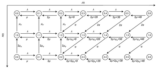
Figure 2. State transition diagram of the Markov chain model on the extended state space $\widehat{S}$.

We observe that $\widehat{S}$ contains a single irreducible class that exactly coincides with the original state space S. Moreover, the transition rates within this irreducible class are identical to those of the original model on S. This implies that the stationary distribution of $\{\widehat{X}(t);t\ge 0\}$, when restricted to this irreducible class, is identical to the stationary distribution π of the original model.

We define the probability vector $\widehat{\mathit{\pi }}$ as

$$\begin{array}{cc}\hfill \widehat{\mathit{\pi }}& =({\widehat{\mathit{\pi }}}_0,{\widehat{\mathit{\pi }}}_1,\dots ,{\widehat{\mathit{\pi }}}_K,\mathbf{0},\mathbf{0},\dots ).\hfill \end{array}$$

Here, each ${\widehat{\mathit{\pi }}}_j$ is defined as

$$\begin{array}{cc}\hfill {\widehat{\mathit{\pi }}}_j& =({\widehat{\pi }}_{0,j},{\widehat{\pi }}_{1,j},\dots ,{\widehat{\pi }}_{v,j}), 0\le j\le K,\hfill \end{array}$$

where

$$\begin{array}{cc}\hfill {\widehat{\pi }}_{i,j}& =\underset{t\to \infty }{lim}Pr(\widehat{X}(t)=(i,j)), (i,j)\in \widehat{S}.\hfill \end{array}$$

Note that ${\widehat{\pi }}_{i,j}=0$ for all transient states $(i,j)\in \widehat{S}\setminus S$. Therefore, $\widehat{\mathit{\pi }}$ is essentially the same as the stationary distribution π of the original model on S, padded with zeros corresponding to the transient states in $\widehat{S}$.

4.2. Upper Bounding Model by Bright and Taylor

We briefly summarize the construction of an LDQBD process $\{\overline{X}(t);t\ge 0\}$ that stochastically dominates $\{\widehat{X}(t);t\ge 0\}$. We begin with the following assumption.

Condition 1.

For all $j\ge 1$, for every $i\in \{0,1,\dots ,v\}$, there exists $n\in \{0,1,\dots ,v\}$ such that

$$\begin{array}{c}\hfill {({\widehat{Q}}_2^{(j)})}_{i,n}>0.\end{array}$$

The following proposition gives a construction of an LDQBD process that stochastically dominates $\{\widehat{X}(t);t\ge 0\}$.

Proposition 1

(Theorem 1 in [8]). Suppose the LDQBD process $\{\widehat{X}(t);t\ge 0\}$ satisfies Condition 1. Define a new LDQBD process $\{\overline{X}(t);t\ge 0\}$ with transition rate matrix $\overline{Q}$ given by

$$\begin{array}{cc}\hfill \overline{Q}& =\left[\begin{array}{cccccc}{\overline{Q}}_1^{(0)}& {\overline{Q}}_0^{(0)}& O& \dots & O& \dots \\ {\overline{Q}}_2^{(1)}& \ddots & \ddots & \ddots & ⋮& \ddots \\ O& \ddots & \ddots & {\overline{Q}}_0^{(K-1)}& O& \ddots \\ ⋮& \ddots & {\overline{Q}}_2^{(K)}& {\overline{Q}}_1^{(K)}& {\overline{Q}}_0^{(K)}& \ddots \\ O& \dots & O& {\overline{Q}}_2^{(K+1)}& {\overline{Q}}_1^{(K+1)}& \ddots \\ ⋮& \ddots & \ddots & \ddots & \ddots & \ddots \end{array}\right],\hfill \end{array}$$

where the block matrices are defined as

$$\begin{array}{cc}\hfill {({\overline{Q}}_0^{(0)})}_{i,n}& ={({\widehat{Q}}_0^{(0)})}_{i,n},\hfill \\ \hfill {({\overline{Q}}_0^{(k)})}_{i,n}& =max\left\{{\displaystyle \frac{{({\widehat{Q}}_0^{(k-1)}\mathbf{1})}_{max}}{M_{k+1}}},{({\widehat{Q}}_0^{(k)})}_{i,n}\right\},\hfill & \hfill & k\ge 1,\hfill \\ \hfill {({\overline{Q}}_2^{(1)})}_{i,n}& =0,\hfill \\ \hfill {({\overline{Q}}_2^{(k)})}_{i,n}& =min\left\{{\displaystyle \frac{{({\widehat{Q}}_2^{(k-1)}\mathbf{1})}_{min}}{M_{k-1}}},{({\widehat{Q}}_2^{(k)})}_{i,n}\right\},\hfill & \hfill & k\ge 2,\hfill \\ \hfill {({\overline{Q}}_1^{(k)})}_{i,n}& ={({\widehat{Q}}_1^{(k)})}_{i,n},\hfill & \hfill & i\ne n,k\ge 0.\hfill \end{array}$$

Here, $M_k$ denotes the number of states in level k, i.e., ${\widehat{S}}_k=\{(i,j)\in \widehat{S}\mid j=k\}$, and ${(\mathit{a})}_{max}$, ${(\mathit{a})}_{min}$ denote the maximum and minimum components of vector a, respectively. Then, the process $\{\overline{X}(t);t\ge 0\}$ stochastically dominates $\{\widehat{X}(t);t\ge 0\}$.

It should be noted that Condition 1 is satisfied for the specific LDQBD process $\{\widehat{X}(t);t\ge 0\}$. Moreover, we observe that $\{\overline{X}(t);t\ge 0\}$ has a single finite irreducible class given by

$$\begin{array}{cc}\hfill \overline{C}& =\left\{(i,j)\mid 0\le i\le v,1\le j\le K+1\right\}.\hfill \end{array}$$

The following corollary is immediate from the stochastic dominance of $\{\overline{X}(t);t\ge 0\}$ over $\{\widehat{X}(t);t\ge 0\}$.

Corollary 1.

Let $({\overline{\mathit{\pi }}}_1,\dots ,{\overline{\mathit{\pi }}}_{K+1})$ denote the stationary distribution on $\overline{C}$, where

$$\begin{array}{cc}\hfill {\overline{\mathit{\pi }}}_j& =({\overline{\pi }}_{0,j},{\overline{\pi }}_{1,j},\dots ,{\overline{\pi }}_{v,j}),1\le j\le K+1,\hfill \end{array}$$

and

$$\begin{array}{cc}\hfill {\overline{\pi }}_{i,j}& =\underset{t\to \infty }{lim}Pr(X(t)=(i,j)),(i,j)\in \overline{C}.\hfill \end{array}$$

If we define the probability vector $\overline{\mathit{\pi }}$ as

$$\begin{array}{cc}\hfill \overline{\mathit{\pi }}& =(\mathbf{0},{\overline{\mathit{\pi }}}_1,\dots ,{\overline{\mathit{\pi }}}_{K+1},\mathbf{0},\dots ),\hfill \end{array}$$

then the following stochastic dominance relation holds.

$$\begin{array}{cc}\hfill \widehat{\mathit{\pi }}& {\le }_s\overline{\mathit{\pi }}.\hfill \end{array}$$

4.3. Alternative Upper Bounding Model

Using Proposition 1, we can obtain the LDQBD process $\{\overline{X}(t);t\ge 0\}$ that stochastically dominates $\{\widehat{X}(t);t\ge 0\}$. However, there are several issues that must be addressed.

• The structure of ${({\overline{Q}}_0^{(k)})}_{i,n}$ does not preserve the transition structure compatible with the recursive approach developed in Phung-Duc and Kawanishi [4]. As a result, we cannot compute the stationary distribution of $\{\overline{X}(t);t\ge 0\}$ using a recurrence relation.

This limitation is a key challenge that we overcome in this paper. In addition, there are the following two issues.

2.

Since the transition rate ${({\overline{Q}}_2^{(k)})}_{i,n}$ is defined as the minimum of ${\left({\widehat{Q}}_2^{(k-1)}\mathbf{1}\right)}_{min}/M_{k-1}$ and ${({\widehat{Q}}_2^{(k)})}_{i,n}$, it may result in a conservative upper bounding LDQBD process.

3.

Similarly, since ${({\overline{Q}}_0^{(k)})}_{i,n}$ is defined as the maximum of ${\left({\widehat{Q}}_0^{(k-1)}\mathbf{1}\right)}_{max}/M_{k+1}$ and ${({\widehat{Q}}_0^{(k)})}_{i,n}$, it may also lead to a large upper bounding process.

To address the second issue, we suppose that $\{\widehat{X}(t);t\ge 0\}$ satisfies Condition 1, and we define the normalized transition weights ${\widehat{w}}_{i,n}^{(k)}$ as

$$\begin{array}{c}\hfill {\widehat{w}}_{i,n}^{(k)}={\displaystyle \frac{{({\widehat{Q}}_2^{(k)})}_{i,n}}{{\sum }_{n\in {\widehat{S}}_{k-1}}{({\widehat{Q}}_2^{(k)})}_{i,n}}}, k\ge 1, i\in {\widehat{S}}_k, n\in {\widehat{S}}_{k-1}.\end{array}$$

Note that ${\sum }_{n\in {\widehat{S}}_{k-1}}{({\widehat{Q}}_2^{(k)})}_{i,n}\ne 0$ by Condition 1.

To resolve the third issue, we define the normalized forward transition weights ${\widehat{z}}_{i,n}^{(k)}$ as

$$\begin{array}{c}\hfill {\widehat{z}}_{i,n}^{(k)}=\left\{\begin{array}{cc}{\displaystyle \frac{{({\widehat{Q}}_0^{(k)})}_{i,n}}{{\sum }_{n\in {\widehat{S}}_{k+1}}{({\widehat{Q}}_0^{(k)})}_{i,n}},}\hfill & \mathrm{if}\sum _{n\in {\widehat{S}}_{k+1}}{({\widehat{Q}}_0^{(k)})}_{i,n}\ne 0,\hfill \\ 0,\hfill & \mathrm{otherwise},\hfill \end{array}\right.k\ge 1,i\in {\widehat{S}}_k,n\in {\widehat{S}}_{k+1}.\end{array}$$

Taking account of the aforementioned issues, we design an alternative LDQBD process that not only stochastically dominates $\{\widehat{X}(t);t\ge 0\}$ but also enables us to compute its stationary distribution using a recurrence relation. The construction is summarized in the following theorem. The proof is provided in Appendix B.

Theorem 1.

Suppose that $\{\widehat{X}(t);t\ge 0\}$ satisfies Condition 1. Let us consider the LDQBD process $\{\check{X}(t);t\ge 0\}$ with transition rate matrix $\check{Q}$ given by

$$\begin{array}{cc}\hfill \check{Q}& =\left[\begin{array}{cccccc}{\check{Q}}_1^{(0)}& {\check{Q}}_0^{(0)}& O& \dots & O& \dots \\ {\check{Q}}_2^{(1)}& \ddots & \ddots & \ddots & ⋮& \ddots \\ O& \ddots & \ddots & {\check{Q}}_0^{(K-1)}& O& \ddots \\ ⋮& \ddots & {\check{Q}}_2^{(K)}& {\check{Q}}_1^{(K)}& {\check{Q}}_0^{(K)}& \ddots \\ O& \dots & O& {\check{Q}}_2^{(K+1)}& {\check{Q}}_1^{(K+1)}& \ddots \\ ⋮& \ddots & \ddots & \ddots & \ddots & \ddots \end{array}\right],\hfill \end{array}$$

where the block matrices are defined as

$$\begin{array}{}\mathrm{(1)}& {({\check{Q}}_0^{(k)})}_{i,n}={({\widehat{Q}}_0^{(k)})}_{i,n},\hfill & k=0,\hfill \mathrm{(2)}& {({\check{Q}}_0^{(k)})}_{i,n}=max\left\{{\delta }_{i,n}{({\widehat{Q}}_0^{(k-1)}\mathbf{1})}_{max},{\widehat{z}}_{i,n}^{(k)}{({\widehat{Q}}_0^{(k-1)}\mathbf{1})}_{max},{({\widehat{Q}}_0^{(k)})}_{i,n}\right\},\hfill & k=1,\hfill \mathrm{(3)}& {({\check{Q}}_0^{(k)})}_{i,n}=max\left\{\begin{array}{c}{\delta }_{i,n}{({\widehat{Q}}_0^{(k-1)}\mathbf{1})}_{max},{\widehat{z}}_{i,n}^{(k)}{({\widehat{Q}}_0^{(k-1)}\mathbf{1})}_{max},\hfill \\ {({\widehat{Q}}_0^{(k)})}_{i,n}+{\delta }_{i,n}\sum _{\begin{array}{c}m\\ m\ne i\end{array}}{({\widehat{Q}}_1^{(k)})}_{i,m}\hfill \end{array}\right\},\hfill & k\ge 2,\hfill \mathrm{(4)}& {({\check{Q}}_2^{(k)})}_{i,n}=0,\hfill & k=1,\hfill \mathrm{(5)}& {({\check{Q}}_2^{(k)})}_{i,n}=min\left\{{\widehat{w}}_{i,n}^{(k)}{({\widehat{Q}}_2^{(k-1)}\mathbf{1})}_{min},{({\widehat{Q}}_2^{(k)})}_{i,n}\right\},\hfill & k\ge 2,\hfill \mathrm{(6)}& {({\check{Q}}_1^{(k)})}_{i,n}={({\widehat{Q}}_1^{(k)})}_{i,n},\hfill & i\ne n,k=0,1,\hfill \mathrm{(7)}& {({\check{Q}}_1^{(k)})}_{i,n}=0,\hfill & i\ne n,k\ge 2.\hfill \end{array}$$

Here, ${\delta }_{i,n}$ denotes the Kronecker delta defined by

$${\delta }_{i,n}=\left\{\begin{array}{cc}1\hfill & \mathit{if}i=n,\hfill \\ 0\hfill & \mathit{otherwise}.\hfill \end{array}\right.$$

Then, the process $\{\check{X}(t);t\ge 0\}$ stochastically dominates $\{\widehat{X}(t);t\ge 0\}$.

Remark 1.

Note that, for $k\ge 2$, the term ${\delta }_{i,n}{\sum }_{\begin{array}{c}m:m\ne i\end{array}}{({\widehat{Q}}_1^{(k)})}_{i,m}$ is added to the transition rate ${({\widehat{Q}}_0^{(k)})}_{i,n}$ in (3). This modification is essential for compensating for the removal of off-diagonal elements in ${\check{Q}}_1^{(k)}$ for $k\ge 2$ (see (7)). As a result of this removal, the only possible nonzero transition rates that preserve the level variable appear at levels $k=0$ and $k=1$, which is the key distinction between $\{\check{X}(t);t\ge 0\}$ and $\{\widehat{X}(t);t\ge 0\}$.

We observe that the LDQBD process $\{\check{X}(t);t\ge 0\}$ has a single finite irreducible class $\check{C}$ given by

$$\begin{array}{cc}\hfill \check{C}& =\{(i,j)\mid 0\le i\le v,1\le j\le K+1\}.\hfill \end{array}$$

All states in $\widehat{S}\setminus \check{C}$ are transient. This leads to the following corollary.

Corollary 2.

Let $({\check{\mathit{\pi }}}_1,\dots ,{\check{\mathit{\pi }}}_{K+1})$ denote the stationary distribution on $\check{C}$, where

$$\begin{array}{cc}\hfill {\check{\mathit{\pi }}}_j& =({\check{\pi }}_{0,j},{\check{\pi }}_{1,j},\dots ,{\check{\pi }}_{v,j}),1\le j\le K+1,\hfill \end{array}$$

and

$$\begin{array}{cc}\hfill {\check{\pi }}_{i,j}& =\underset{t\to \infty }{lim}Pr(X(t)=(i,j)),(i,j)\in \check{C}.\hfill \end{array}$$

Define the probability vector $\check{\mathit{\pi }}$ as

$$\begin{array}{cc}\hfill \check{\mathit{\pi }}& =(\mathbf{0},{\check{\mathit{\pi }}}_1,\dots ,{\check{\mathit{\pi }}}_{K+1},\mathbf{0},\dots ),\hfill \end{array}$$

where the zero vectors correspond to the transient states in $\widehat{S}\setminus \check{C}$. Then, the following stochastic dominance relation holds.

$$\begin{array}{cc}\hfill \widehat{\mathit{\pi }}& {\le }_s\check{\mathit{\pi }}.\hfill \end{array}$$

Remark 2.

Note that the single irreducible class $\check{C}=\{(i,j)\mid 0\le i\le v,1\le j\le K+1\}$ of the upper bounding model does not include the set of states $\{(i,0)\mid 0\le i\le v\}$. Therefore, the transition rates at level $k=0$ do not affect the stationary distribution of $\{\check{X}(t);t\ge 0\}$. As a result, the transition structure of $\{\check{X}(t);t\ge 0\}$ allows the computation of $\check{\mathit{\pi }}$, which stochastically dominates $\widehat{\mathit{\pi }}$ and is also compatible with the recursive computation method proposed by Phung-Duc and Kawanishi [4].

Example 1.

As an illustrative example, let us consider the case when $k=2$ in Figure 2. In this case, we have

$$\begin{array}{c}\hfill {\widehat{Q}}_0^{(2)}=\left(\begin{array}{ccc}\lambda & 0& 0\\ 0& \lambda & 0\\ 0& 0& \lambda \end{array}\right),{({\widehat{Q}}_0^{(1)}\mathbf{1})}_{max}=\lambda .\end{array}$$

If we apply Proposition 1, then ${\overline{Q}}_0^{(2)}$ is obtained as follows:

$$\begin{array}{c}\hfill {\overline{Q}}_0^{(2)}=\left(\begin{array}{ccc}\lambda & \lambda /3& \lambda /3\\ \lambda /3& \lambda & \lambda /3\\ \lambda /3& \lambda /3& \lambda \end{array}\right).\end{array}$$

Since the row sums of ${\overline{Q}}_0^{(2)}$ are greater than or equal to $\lambda ={({\widehat{Q}}_0^{(1)}\mathbf{1})}_{max}$, the condition ensuring that $\{\overline{X}(t);t\ge 0\}$ stochastically dominates $\{\widehat{X}(t);t\ge 0\}$ is satisfied. However, due to the presence of off-diagonal components such as $\lambda /3$, the resulting transition structure is no longer compatible with the recurrence-based method proposed in Phung-Duc and Kawanishi [4]. In contrast, if we apply Theorem 1, then ${\check{Q}}_0^{(2)}$ becomes

$$\begin{array}{c}\hfill {\check{Q}}_0^{(2)}=\left(\begin{array}{ccc}\lambda & 0& 0\\ 0& \lambda +{\mu }_v& 0\\ 0& 0& \lambda +2{\mu }_v\end{array}\right).\end{array}$$

Since all the off-diagonal components of ${\check{Q}}_0^{(2)}$ are zero, the recurrence-based method can be applied in this case.

Figure 3 illustrates the state transition diagram of the process $\{\check{X}(t);t\ge 0\}$ on $\widehat{S}$ when l = 2, v = 2, and K = 5. It also illustrates the differences in the transition structure before and after applying Theorem 1. The transition rate μ_v from state (1, 2) to state (0, 2) has been removed and reassigned to the transition rate leading to state (1, 3). Similarly, the transition rate 2μ_v from state (2, 2) to state (1, 2) has been removed and reassigned to the transition rate leading to state (2, 3). Additionally, transitions represented by dashed arrows with rate λ are newly added.

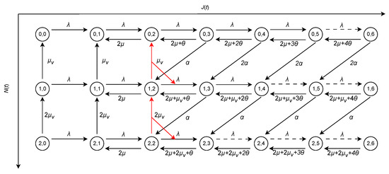
Figure 3. State space extension model that gives a stochastic upper bound. Red arrows indicate transitions whose rates have been reassigned: μ_v from (1, 2) → (0, 2) to (1, 2) → (1, 3), and 2μ_v from (2, 2) → (1, 2) to (2, 2) → (2, 3). Dashed arrows indicate additional transitions with rate λ.

Since ${({\check{Q}}_1^{(k)})}_{i,n}=0$ for k ≥ 2 and i ≠ n, the process $\{\check{X}(t);t\ge 0\}$ in Theorem 1 has a transition structure that enables computation of the stationary distribution by recurrence relations, as proposed in Phung-Duc and Kawanishi [4].

4.4. Balance Equations of Stationary Distribution on $\check{C}$

We now derive the global balance equations that characterize the stationary distribution $({\check{\mathit{\pi }}}_1,{\check{\mathit{\pi }}}_2,\dots ,{\check{\mathit{\pi }}}_{K+1})$ on the finite irreducible class $\check{C}$ of the process $\{\check{X}(t);t\ge 0\}$.

For i = 0 and 1 < j ≤ K + 1, the global balance equations for ${\check{\pi }}_{0,j}$ are given by

$$\begin{array}{cc}\hfill \left[{({\check{Q}}_0^{(j)})}_{0,0}+\sum _{n\in {\widehat{S}}_{j-1}}{({\check{Q}}_2^{(j)})}_{0,n}\right]{\check{\pi }}_{0,j}=& {({\check{Q}}_0^{(j-1)})}_{0,0}{\check{\pi }}_{0,j-1}\hfill \\ & +{({\check{Q}}_2^{(j+1)})}_{0,0}·{\check{\pi }}_{0,j+1},1<j<K+1,\hfill \end{array}$$

(8)

$$\begin{array}{cc}\hfill \left[\sum _{n\in {\widehat{S}}_{j-1}}{({\check{Q}}_2^{(j)})}_{0,n}\right]{\check{\pi }}_{0,j}& ={({\check{Q}}_0^{(j-1)})}_{0,0}{\check{\pi }}_{0,j-1},j=K+1.\hfill \end{array}$$

(9)

For 1 ≤ i ≤ v and 1 < j ≤ K + 1, the global balance equations for ${\check{\pi }}_{i,j}$ are given by

$$\begin{array}{cc}\hfill \left[{({\check{Q}}_0^{(j)})}_{i,i}+\sum _{n\in {\widehat{S}}_{j-1}}{({\check{Q}}_2^{(j)})}_{i,n}\right]{\check{\pi }}_{i,j}& ={({\check{Q}}_0^{(j-1)})}_{i,i}{\check{\pi }}_{i,j-1}+{({\check{Q}}_2^{(j+1)})}_{i,i}·{\check{\pi }}_{i,j+1}\hfill \\ & +{({\check{Q}}_2^{(j+1)})}_{i-1,i}·{\check{\pi }}_{i-1,j+1},1<j<K+1,\hfill \end{array}$$

(10)

$$\begin{array}{cc}\hfill \left[\sum _{n\in {\widehat{S}}_{j-1}}{({\check{Q}}_2^{(j)})}_{i,n}\right]{\check{\pi }}_{i,j}& ={({\check{Q}}_0^{(j-1)})}_{i,i}{\check{\pi }}_{i,j-1},j=K+1.\hfill \end{array}$$

(11)

Note that the above equations do not cover the case where j = 1. To address this, we define a subset ${\check{C}}_i$ of the irreducible class $\check{C}$ as follows.

$$\begin{array}{c}\hfill {\check{C}}_i=\left\{(n,j)\mid i\le n\le v,1\le j\le K+1\right\},1\le i\le v.\end{array}$$

From the global balance between ${\check{C}}_i$ and its complement $\check{C}\setminus {\check{C}}_i$, we obtain

$$\begin{array}{c}\hfill i{\mu }_v{\check{\pi }}_{i,1}=\sum _{j=1}^{K+1}{({\check{Q}}_2^{(j)})}_{i-1,i}·{\check{\pi }}_{i-1,j}, 1\le i\le v.\end{array}$$

The base case ${\check{\pi }}_{0,1}$ is determined from the normalization condition given by

$$\begin{array}{cc}\hfill \sum _{i=0}^v\sum _{j=1}^{K+1}{\check{\pi }}_{i,j}& =1.\hfill \end{array}$$

From the above balance equations and normalization condition, we see that the stationary distribution $({\check{\mathit{\pi }}}_1,{\check{\mathit{\pi }}}_2,\dots ,{\check{\mathit{\pi }}}_{K+1})$ is uniquely determined.

4.5. Construction of Recurrence Relation

We now construct a recurrence relation for the stationary distribution components ${\check{\pi }}_{i,j}$ on $\check{C}$. We begin with the case i = 0. From the global balance Equation (9), we observe that ${\check{\pi }}_{0,K+1}$ is determined once ${\check{\pi }}_{0,K}$ is given. Next, using (8) for j = K, we find that ${\check{\pi }}_{0,K}$ is determined if ${\check{\pi }}_{0,K-1}$ is known. Repeating this backward process for j = K − 1, K − 2, …, 2, we see that ${\check{\pi }}_{0,j+1}$ is recursively determined from ${\check{\pi }}_{0,j}$. Therefore, starting from the initial value ${\check{\pi }}_{0,1}$, we obtain the following recurrence relation. The proof is omitted as it is an immediate consequence of the global balance equations.

Lemma 1.

The sequence ${\check{\pi }}_{0,j}$$(1<j\le K+1)$ satisfies the recurrence relation

$$\begin{array}{cc}\hfill {\check{\pi }}_{0,j}& ={\check{b}}_{0,j}·{\check{\pi }}_{0,j-1}, 1<j\le K+1,\hfill \end{array}$$

where the coefficient ${\check{b}}_{0,j}$ is given by

$$\begin{array}{cc}\hfill {\check{b}}_{0,j}& ={\displaystyle \frac{{({\check{Q}}_0^{(j-1)})}_{0,0}}{{\sum }_{n\in {\widehat{S}}_{j-1}}{({\check{Q}}_2^{(j)})}_{0,n}+{({\check{Q}}_0^{(j)})}_{0,0}·{\check{c}}_{0,j}}}, 1<j\le K+1,\hfill \end{array}$$

and the auxiliary coefficient ${\check{c}}_{0,j}$ is recursively defined as

$$\begin{array}{cc}\hfill {\check{c}}_{0,j}& =\left\{\begin{array}{cc}0,\hfill & j=K+1,\hfill \\ {\displaystyle \frac{{({\check{Q}}_2^{(j+1)})}_{0,1}+{({\check{Q}}_0^{(j+1)})}_{0,0}·{\check{c}}_{0,j+1}}{{\sum }_{n\in {\widehat{S}}_j}{({\check{Q}}_2^{(j+1)})}_{0,n}+{({\check{Q}}_0^{(j+1)})}_{0,0}·{\check{c}}_{0,j+1}},}\hfill & 1<j<K+1.\hfill \end{array}\right.\hfill \end{array}$$

Remark 3.

Lemma 1 implies that all ${\check{\pi }}_{0,j}$ for $1<j\le K+1$ can be expressed in terms of the initial value ${\check{\pi }}_{0,1}$. Moreover, from the balance equation between the subset ${\check{C}}_1$ and its complement, we have

$$\begin{array}{c}\hfill {\mu }_v{\check{\pi }}_{1,1}=\sum _{j=1}^{K+1}{({\check{Q}}_2^{(j)})}_{0,1}·{\check{\pi }}_{0,j}.\end{array}$$

Since the right-hand side depends only on ${\check{\pi }}_{0,j}$ for $j>0$, which are themselves recursively determined by ${\check{\pi }}_{0,1}$, it follows that ${\check{\pi }}_{1,1}$ is also determined by ${\check{\pi }}_{0,1}$.

Remark 4.

As in Phung-Duc et al. [2] and Ren et al. [3], the recurrence relations in Lemma 1 can be reformulated without using the auxiliary coefficient ${\check{c}}_{0,j}$ as follows.

$$\begin{array}{cc}\hfill {\check{b}}_{0,j}& =\left\{\begin{array}{cc}{\displaystyle \frac{{({\check{Q}}_0^{(j-1)})}_{0,0}}{{\sum }_{n\in {\widehat{S}}_{j-1}}{({\check{Q}}_2^{(j)})}_{0,n}},}\hfill & j=K+1,\hfill \\ {\displaystyle \frac{{({\check{Q}}_0^{(j-1)})}_{0,0}}{{({\check{Q}}_0^{(j)})}_{0,0}+{\sum }_{n\in {\widehat{S}}_{j-1}}{({\check{Q}}_2^{(j)})}_{0,n}-{({\check{Q}}_2^{(j+1)})}_{0,0}·{\check{b}}_{0,j+1}},}\hfill & 1<j<K+1.\hfill \end{array}\right.\hfill \end{array}$$

These recurrence relations involve subtraction, which may lead to numerical instability. In contrast, the formulation given in Lemma 1 avoids subtraction and is numerically more stable.

Next, we consider the recurrence relation for ${\check{\pi }}_{i,j}$ with 1 ≤ i ≤ v. Using the global balance Equations (10) and (11), we obtain a similar recursive structure as follows. The proof is again omitted, as it is an immediate consequence of these equations.

Lemma 2.

For $1\le i\le v$ and $1<j\le K+1$, ${\check{\pi }}_{i,j}$ satisfies the recurrence relation

$$\begin{array}{c}\hfill {\check{\pi }}_{i,j}={\check{a}}_{i,j}+{\check{b}}_{i,j}·{\check{\pi }}_{i,j-1},\end{array}$$

where the coefficients are defined as

$$\begin{array}{cc}\hfill {\check{a}}_{i,j}& =\left\{\begin{array}{cc}0,\hfill & j=K+1,\hfill \\ {\displaystyle \frac{{({\check{Q}}_2^{(j+1)})}_{i,i}·{\check{a}}_{i,j+1}+{({\check{Q}}_2^{(j+1)})}_{i-1,i}·{\check{\pi }}_{i-1,j+1}}{{\sum }_{n\in {\widehat{S}}_{j-1}}{({\check{Q}}_2^{(j)})}_{i,n}+{({\check{Q}}_0^{(j)})}_{i,i}·{\check{c}}_{i,j}},}\hfill & 1<j<K+1,\hfill \end{array}\right.\hfill \\ \hfill {\check{b}}_{i,j}& ={\displaystyle \frac{{({\check{Q}}_0^{(j-1)})}_{i,i}}{{\sum }_{n\in {\widehat{S}}_{j-1}}{({\check{Q}}_2^{(j)})}_{i,n}+{({\check{Q}}_0^{(j)})}_{i,i}·{\check{c}}_{i,j}}},1<j\le K+1,\hfill \\ \hfill {\check{c}}_{i,j}& =\left\{\begin{array}{cc}0,\hfill & j=K+1,\hfill \\ {\displaystyle \frac{{({\check{Q}}_2^{(j+1)})}_{i,i+1}+{({\check{Q}}_0^{(j+1)})}_{i,i}·{\check{c}}_{i,j+1}}{{\sum }_{n\in {\widehat{S}}_j}{({\check{Q}}_2^{(j+1)})}_{i,n}+{({\check{Q}}_0^{(j+1)})}_{i,i}·{\check{c}}_{i,j+1}},}\hfill & 1<j<K+1,\hfill \end{array}\right.\hfill \end{array}$$

with the convention that ${({\check{Q}}_2^{(j+1)})}_{v,v+1}=0$ for $1<j<K+1$.

Remark 5.

From Lemma 2, each ${\check{\pi }}_{i,j}$$(1\le i\le v,1<j\le K+1)$ is expressed in terms of ${\check{\pi }}_{i,j-1}$ and ${\check{\pi }}_{i-1,j+1}$. Combined with the balance equation

$$\begin{array}{c}\hfill i{\mu }_v{\check{\pi }}_{i,1}=\sum _{j=1}^{K+1}{({\check{Q}}_2^{(j)})}_{i-1,i}·{\check{\pi }}_{i-1,j},\end{array}$$

we find that ${\check{\pi }}_{i,1}$ depends on ${\check{\pi }}_{i-1,j}$ for $j>0$. Proceeding inductively, and using Lemmas 1 and 2, all components ${\check{\pi }}_{i,j}$ for $0\le i\le v,1\le j\le K+1$ are recursively determined from the initial value ${\check{\pi }}_{0,1}$.

Remark 6.

The total number of states in $\check{C}$ is

$$\begin{array}{c}\hfill (v+1)(K+1)=(v+1)(l+v+\mathsf{\Delta }+1),\end{array}$$

which scales as $O(v^2)$ and is asymptotically of the same order as that of the original model. The recurrence-based method computes ${\check{\pi }}_{i,j}$ for all states in $\check{C}$ using the coefficients ${\check{a}}_{i,j}$, ${\check{b}}_{i,j}$, and ${\check{c}}_{i,j}$. The total space required to store these coefficients is

$$\begin{array}{c}\hfill v\times K+(v+1)\times K+(v+1)\times K=(3v+2)\times (l+v+\mathsf{\Delta }),\end{array}$$

which grows as $O(v^2)$. This is asymptotically smaller than the space requirement for storing $R^{(j)}$ ($1\le j\le K$) in the matrix analytic methods. For each $i\in \{0,1,\dots ,v\}$, computing ${\check{a}}_{i,j}$, ${\check{b}}_{i,j}$, and ${\check{c}}_{i,j}$ involves at most $(v+1)$ additions in the denominators of the coefficients. Consequently, the total time required to obtain all coefficients is at most

$$\begin{array}{c}\hfill 3\times (v+1)\times (v+1)\times (K+1)=3{(v+1)}^2\times (l+v+\mathsf{\Delta }+1),\end{array}$$

which grows as $O(v^3)$. This is also asymptotically smaller than the $O(v^4)$ complexity of computing $R^{(j)}$ in the matrix analytic methods.

5. Lower Bounding Model

In constructing the upper bounding LDQBD process, we used J(t) as the level variable, defined as the total number of jobs being processed by legacy servers and those waiting in the queue at time t. A natural idea for deriving a lower bounding LDQBD process is to reverse the direction of the level variable, i.e., to replace J(t) with K − J(t). However, such a straightforward reversal does not yield a LDQBD process that satisfies Condition 1, which is essential for applying the method in [8].

To overcome this issue, we redefine the level variable. Instead of J(t), we consider $\tilde{J}(t)$ as the total number of jobs in the system at time t, including those being processed by both legacy and virtual servers as well as those waiting in the queue. Then, we define the level variable by ${\tilde{J}}^{\prime }(t)=K-\tilde{J}(t)$ and consider the LDQBD process $\{\tilde{X}(t)=(\tilde{N}(t),{\tilde{J}}^{\prime }(t));t\ge 0\}$, where $\tilde{N}(t)$ denotes the number of active virtual servers that have completed their setup at time t. The state space $\tilde{S}$ of the process $\{\tilde{X}(t)=(\tilde{N}(t),{\tilde{J}}^{\prime }(t));t\ge 0\}$ is defined by

$$\begin{array}{c}\hfill \tilde{S}=\left\{(i,j^{\prime })|0\le i\le v,0\le j^{\prime }\le K-i\right\}.\end{array}$$

To derive a lower bounding model for the original process, we construct a LDQBD process with the level variable reversed and appropriately redefined. Let $\tilde{Q}$ denote the transition rate matrix of $\{\tilde{X}(t)=(\tilde{N}(t),{\tilde{J}}^{\prime }(t));t\ge 0\}$ on the state space $\tilde{S}$. Then, $\tilde{Q}$ is constructed so that it has a block tridiagonal structure and is given by

$$\begin{array}{cc}\hfill \tilde{Q}& =\left[\begin{array}{ccccc}{\tilde{Q}}_1^{(0)}& {\tilde{Q}}_0^{(0)}& O& \dots & O\\ {\tilde{Q}}_2^{(1)}& {\tilde{Q}}_1^{(1)}& {\tilde{Q}}_0^{(1)}& \ddots & ⋮\\ O& {\tilde{Q}}_2^{(2)}& {\tilde{Q}}_1^{(2)}& \ddots & O\\ ⋮& \ddots & \ddots & \ddots & {\tilde{Q}}_0^{(K-1)}\\ O& \dots & O& {\tilde{Q}}_2^{(K)}& {\tilde{Q}}_1^{(K)}\end{array}\right].\hfill \end{array}$$

Block matrices ${\tilde{Q}}_0^{(j^{\prime })}(0\le j^{\prime }\le K-1),{\tilde{Q}}_1^{(j^{\prime })}(0\le j^{\prime }\le K),{\tilde{Q}}_2^{(j^{\prime })}(1\le j^{\prime }\le K)$ of $\tilde{Q}$ are transition rate matrices, which represent transitions that increase, maintain, and decrease the level variable ${\tilde{J}}^{\prime }(t)$ by one, respectively. The block matrices of $\tilde{Q}$ are presented explicitly in Appendix A. As an example, we show the state transition diagram for $\tilde{S}$ when l = 2, v = 2, and K = 5 in Figure 4.

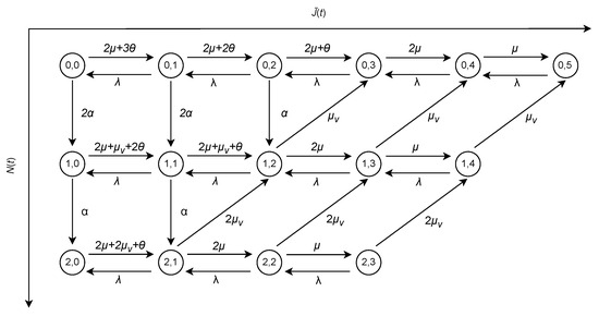
Figure 4. State transition diagram of the model on state space $\tilde{S}$.

Remark 7.

In contrast to the upper bounding model, the level variable in the lower bounding model increases due to the departure of jobs rather than their arrival. This reversal reflects the fact that the state $(i,j^{\prime })$ with smaller $j^{\prime }$ corresponds to a larger number of jobs in the system.

Since $\tilde{S}$ is finite, and $\tilde{Q}$ is irreducible, the stationary distribution $\tilde{\mathit{\pi }}$ of $\{\tilde{X}(t)=(\tilde{N}(t),{\tilde{J}}^{\prime }(t));t\ge 0\}$ uniquely exists and is given by the solution of the following system of linear equations.

$$\begin{array}{c}\hfill \tilde{\mathit{\pi }}\tilde{Q}=\mathbf{0},\tilde{\mathit{\pi }}\mathbf{1}=1.\end{array}$$

The stationary distribution can be partitioned as $\tilde{\mathit{\pi }}=({\tilde{\mathit{\pi }}}_0,{\tilde{\mathit{\pi }}}_1,\dots ,{\tilde{\mathit{\pi }}}_K)$, where

$$\begin{array}{cc}\hfill {\tilde{\mathit{\pi }}}_j& =({\tilde{\pi }}_{0,j},{\tilde{\pi }}_{1,j},\dots ,{\tilde{\pi }}_{min\{K-j^{\prime },v\},j^{\prime }}),0\le j^{\prime }\le K,\hfill \end{array}$$

and

$$\begin{array}{cc}\hfill {\tilde{\pi }}_{i,j^{\prime }}& =\underset{t\to \infty }{lim}Pr(\tilde{X}(t)=(i,j^{\prime })),(i,j^{\prime })\in \tilde{S}.\hfill \end{array}$$

5.1. Partial Order Relation on $\tilde{S}$

To compare the states based on the number of jobs in the system, we define a partial order on the state space $\tilde{S}$ that reflects the reversed level structure.

Definition 5.

For two states $(i_1,j_1^{\prime }),(i_2,j_2^{\prime })\in \tilde{S}$, we write $(i_1,j_1^{\prime })\prec (i_2,j_2^{\prime })$ if and only if

$$\begin{array}{c}\hfill j_1^{\prime }<j_2^{\prime }.\end{array}$$

Definition 6.

For two states $(i_1,j_1^{\prime })\in \tilde{S}$ and $(i_2,j_2^{\prime })\in \tilde{S}$, we write $(i_1,j_1^{\prime })⪯(i_2,j_2^{\prime })$ which means that the following condition is satisfied.

$$\begin{array}{c}\hfill (i_1,j_1^{\prime })=(i_2,j_2^{\prime })\mathrm{or}(i_1,j_1^{\prime })\prec (i_2,j_2^{\prime }).\end{array}$$

Remark 8.

Note that the partial order relation is defined in terms of the level variable $j^{\prime }$, not the actual number of jobs in the system. In our construction, $j^{\prime }=K-j$, where j denotes the number of jobs in the system. Therefore, the strict inequality $j_1^{\prime }<j_2^{\prime }$ is equivalent to

$$\begin{array}{cc}\hfill K-j_1<K-j_2& \iff j_1>j_2.\hfill \end{array}$$

In other words, $(i_1,j_1^{\prime })\prec (i_2,j_2^{\prime })$ holds if and only if the number of jobs in the system in the first state is strictly greater than that in the second.

5.2. Stochastic Dominance on $\tilde{S}$

Let $\tilde{X}$ and $\tilde{Y}$ be random variables taking values in the partially ordered set $\tilde{S}$ with the order relation ⪯. We define stochastic dominance in terms of increasing functions on $\tilde{S}$.

Definition 7.

We say that $\tilde{X}$ is stochastically dominated by $\tilde{Y}$ if for every function $\tilde{f}:\tilde{S}\to \mathbb{R}$ that is non-decreasing with respect to ⪯, the following holds.

$$\begin{array}{c}\hfill \sum _{(i,j^{\prime })\in \tilde{S}}\tilde{f}((i,j^{\prime }))Pr(\tilde{X}=(i,j^{\prime }))\le \sum _{(i,j^{\prime })\in \tilde{S}}\tilde{f}((i,j^{\prime }))Pr(\tilde{Y}=(i,j^{\prime })).\end{array}$$

We write $\tilde{X}{\le }_s\tilde{Y}$ if $\tilde{X}$ is stochastically dominated by $\tilde{Y}$.

5.3. Stochastically Dominating LDQBD for $\{\tilde{X}(t);t\ge 0\}$

We construct an LDQBD process that stochastically dominates $\{\tilde{X}(t);t\ge 0\}$. Recall that the level variable ${\tilde{J}}^{\prime }(t)$ is defined by ${\tilde{J}}^{\prime }(t)=K-\tilde{J}(t)$, where $\tilde{J}(t)$ is the number of jobs in the system at time t. This means that the level increases as the number of jobs decreases. Therefore, when an LDQBD process stochastically dominates $\{\tilde{X}(t);t\ge 0\}$ with respect to this level variable, it provides a lower bound in terms of the number of jobs in the system.

To construct such a process, we again apply the framework proposed by Bright and Taylor [8], which enables us to construct an LDQBD process that stochastically dominates $\{\tilde{X}(t);t\ge 0\}$ under a sufficient condition. Unlike the upper bounding model, we do not consider an LDQBD process on an extended state space that includes additional transient states while preserving the same stationary distribution as $\tilde{\mathit{\pi }}$. However, the following condition plays a crucial role in ensuring the applicability of their method as the upper bounding models.

Condition 2.

For all $k^{\prime }\in \{1,2,\dots ,K\}$ and $i\in \{0,1,\dots ,min\{K-k^{\prime },v\}\}$, there exists $n\in \{0,1,\dots ,min\{K-k^{\prime }+1,v\}\}$ such that

$$\begin{array}{c}\hfill {({\tilde{Q}}_2^{(k^{\prime })})}_{i,n}>0.\end{array}$$

For simplicity, we construct a lower bounding model in the case of K > l + v. We obtain the following theorem for the LDQBD process $\{\tilde{X}(t);t\ge 0\}$ under Condition 2. The proof is provided in Appendix B.

Theorem 2.

Suppose that $K>l+v$ and $\{\tilde{X}(t);t\ge 0\}$ satisfies Condition 2. Define the normalized transition weights

$$\begin{array}{cc}\hfill {\tilde{z}}_{i,n}^{(k^{\prime })}& ={\displaystyle \frac{{({\tilde{Q}}_0^{(k^{\prime })})}_{i,n}}{{\sum }_{n\in {\tilde{S}}_{k^{\prime }+1}}{({\tilde{Q}}_0^{(k^{\prime })})}_{i,n}}},{\tilde{w}}_{i,n}^{(k^{\prime })}={\displaystyle \frac{{({\tilde{Q}}_2^{(k^{\prime })})}_{i,n}}{{\sum }_{n\in {\tilde{S}}_{k^{\prime }-1}}{({\tilde{Q}}_2^{(k^{\prime })})}_{i,n}}},\hfill \end{array}$$

where ${\tilde{S}}_k=\{(i,j^{\prime })\in \tilde{S}\mid j^{\prime }=k\}$.

Let $\{\tilde{\tilde{X}}(t);t\ge 0\}$ be an LDQBD process with transition rate matrix

$$\begin{array}{c}\hfill \tilde{\tilde{Q}}=\left[\begin{array}{ccccc}{\tilde{\tilde{Q}}}_1^{(0)}& {\tilde{\tilde{Q}}}_0^{(0)}& O& \dots & O\\ {\tilde{\tilde{Q}}}_2^{(1)}& {\tilde{\tilde{Q}}}_1^{(1)}& {\tilde{\tilde{Q}}}_0^{(1)}& \ddots & ⋮\\ O& {\tilde{\tilde{Q}}}_2^{(2)}& {\tilde{\tilde{Q}}}_1^{(2)}& \ddots & O\\ ⋮& \ddots & \ddots & \ddots & {\tilde{\tilde{Q}}}_0^{(K-1)}\\ O& \dots & O& {\tilde{\tilde{Q}}}_2^{(K)}& {\tilde{\tilde{Q}}}_1^{(K)}\end{array}\right],\end{array}$$

where the block matrices are defined as

$$\begin{array}{}\mathrm{(12)}& {({\tilde{\tilde{Q}}}_0^{(k^{\prime })})}_{i,n}={({\tilde{Q}}_0^{(k^{\prime })})}_{i,n},\hfill & k^{\prime }=0,\hfill \mathrm{(13)}& {({\tilde{\tilde{Q}}}_0^{(k^{\prime })})}_{i,n}=max\left\{{\tilde{z}}_{i,n}^{(k^{\prime })}{({\tilde{Q}}_0^{(k^{\prime }-1)}\mathbf{1})}_{max},{({\tilde{Q}}_0^{(k^{\prime })})}_{i,n}\right\},\hfill & k^{\prime }=1,\hfill \mathrm{(14)}& \hfill {({\tilde{\tilde{Q}}}_0^{(k^{\prime })})}_{i,n}=max\left\{\begin{array}{c}{\tilde{z}}_{i,n}^{(k^{\prime })}{({\tilde{Q}}_0^{(k^{\prime }-1)}\mathbf{1})}_{max},\hfill \\ {({\tilde{Q}}_0^{(k^{\prime })})}_{i,n}+{\delta }_{i,n}\sum _{\begin{array}{c}m\\ m\ne i\end{array}}{({\tilde{Q}}_1^{(k^{\prime })})}_{i,m}\hfill \end{array}\right\},& 2\le k^{\prime }\le K-1,\hfill \mathrm{(15)}& {({\tilde{\tilde{Q}}}_2^{(k^{\prime })})}_{i,n}=0,\hfill & k^{\prime }=1,\hfill \mathrm{(16)}& {({\tilde{\tilde{Q}}}_2^{(k^{\prime })})}_{i,n}=min\left\{{\tilde{w}}_{i,n}^{(k^{\prime })}{({\tilde{Q}}_2^{(k^{\prime }-1)}\mathbf{1})}_{min},{({\tilde{Q}}_2^{(k^{\prime })})}_{i,n}\right\},\hfill & 2\le k^{\prime }\le K,\hfill \mathrm{(17)}& {({\tilde{\tilde{Q}}}_1^{(k^{\prime })})}_{i,n}={({\tilde{Q}}_1^{(k^{\prime })})}_{i,n},\hfill & i\ne n,k^{\prime }=0,1,\hfill \mathrm{(18)}& {({\tilde{\tilde{Q}}}_1^{(k^{\prime })})}_{i,n}=0,\hfill & i\ne n,2\le k^{\prime }\le K.\hfill \end{array}$$

Then, $\{\tilde{\tilde{X}}(t);t\ge 0\}$ stochastically dominates $\{\tilde{X}(t);t\ge 0\}$.

Remark 9.

Due to the transition structure of $\tilde{Q}$, we have ${\sum }_{n\in {\tilde{S}}_{k^{\prime }+1}}{({\tilde{Q}}_0^{(k^{\prime })})}_{i,n}\ne 0$ for all $k^{\prime }\in \{0,1,\dots ,K-1\}$ and $i\in \{0,1,\dots ,min\{K-k^{\prime },v\}\}$. Since Condition 2 is satisfied for $\tilde{Q}$, we also have ${\sum }_{n\in {\tilde{S}}_{k^{\prime }-1}}{({\tilde{Q}}_2^{(k^{\prime })})}_{i,n}\ne 0$ for all $k^{\prime }\in \{1,2,\dots ,K\}$ and $i\in \{0,1,\dots ,min\{K-k^{\prime },v\}\}$.

Remark 10.

The transition rate ${({\tilde{\tilde{Q}}}_1^{(k^{\prime })})}_{i,n}$ is set to zero for $2\le k^{\prime }\le K$ in order to preserve the transition structure that enables the computation of the stationary distribution of $\{\tilde{\tilde{X}}(t);t\ge 0\}$ via recurrence relations. To ensure stochastic dominance over $\{\tilde{X}(t);t\ge 0\}$, the term ${\delta }_{i,n}{\displaystyle \sum _{m\ne i}}{({\tilde{Q}}_1^{(k^{\prime })})}_{i,m}$ is added to the transition rate ${({\tilde{Q}}_0^{(k^{\prime })})}_{i,n}$.

Remark 11.

The process $\{\tilde{\tilde{X}}(t);t\ge 0\}$ has a single irreducible class given by

$$\begin{array}{c}\hfill \tilde{\tilde{C}}=\left\{(i,j^{\prime })\in \tilde{S}\mid 0\le i\le v,1\le j^{\prime }\le K-i\right\}.\end{array}$$

All other states in $\tilde{S}\setminus \tilde{\tilde{C}}$ are transient. In particular, all states with level $j^{\prime }=0$ are transient, and hence their stationary probabilities are equal to zero. It should be noted that the assumption of strict inequality $K>l+v$ is essential to obtain the single irreducible class.

Corollary 3.

Let $({\widetilde{\tilde{\mathit{\pi }}}}_1,{\widetilde{\tilde{\mathit{\pi }}}}_2,\dots ,{\widetilde{\tilde{\mathit{\pi }}}}_K)$ denote the stationary distribution of the process $\{\tilde{\tilde{X}}(t);t\ge 0\}$ on the irreducible class $\tilde{\tilde{C}}$, where

$$\begin{array}{cc}\hfill {\widetilde{\tilde{\mathit{\pi }}}}_{j^{\prime }}& =({\tilde{\tilde{\pi }}}_{0,j^{\prime }},{\tilde{\tilde{\pi }}}_{1,j^{\prime }},\dots ,{\tilde{\tilde{\pi }}}_{min\{K-j^{\prime },v\},j^{\prime }}),1\le j^{\prime }\le K,\hfill \end{array}$$

and

$$\begin{array}{cc}\hfill {\tilde{\tilde{\pi }}}_{i,j^{\prime }}& =\underset{t\to \infty }{lim}Pr(\tilde{\tilde{X}}(t)=(i,j^{\prime })),(i,j^{\prime })\in \tilde{\tilde{C}}.\hfill \end{array}$$

If we define the probability vector $\widetilde{\tilde{\mathit{\pi }}}$ on the entire state space $\tilde{S}$ by

$$\begin{array}{c}\hfill \widetilde{\tilde{\mathit{\pi }}}=(0,{\widetilde{\tilde{\mathit{\pi }}}}_1,{\widetilde{\tilde{\mathit{\pi }}}}_2,\dots ,{\widetilde{\tilde{\mathit{\pi }}}}_K),\end{array}$$

then the following stochastic dominance relation holds:

$$\begin{array}{c}\hfill \tilde{\mathit{\pi }}{\le }_s\widetilde{\tilde{\mathit{\pi }}}.\end{array}$$

Example 2.

As a concrete example, let us consider the case where $k^{\prime }=3$ and $k^{\prime }=4$ in Figure 4. In these cases, the original block matrices ${\tilde{Q}}_0^{(3)}$ and ${\tilde{Q}}_0^{(4)}$ are given by

$$\begin{array}{cc}\hfill {\tilde{Q}}_0^{(3)}& =\left(\begin{array}{cc}2\mu & 0\\ {\mu }_v& \mu \\ 0& 2{\mu }_v\end{array}\right),{\tilde{Q}}_0^{(4)}=\left(\begin{array}{c}\mu \\ {\mu }_v\end{array}\right).\hfill \end{array}$$

Applying Theorem 2, we obtain the modified block matrices ${\tilde{\tilde{Q}}}_0^{(3)}$ and ${\tilde{\tilde{Q}}}_0^{(4)}$ as follows:

$$\begin{array}{cc}\hfill {\tilde{\tilde{Q}}}_0^{(3)}& =\left(\begin{array}{cc}\ast & 0\\ \ast & \ast \\ 0& \ast \end{array}\right),{\tilde{\tilde{Q}}}_0^{(4)}=\left(\begin{array}{c}\ast \\ \ast \end{array}\right).\hfill \end{array}$$

Here, ∗ denotes certain positive values that satisfy the conditions specified in Theorem 2.

In Figure 5, we illustrate the transition structure of the process before and after applying Theorem 2. We observe that the transition labeled α from state (0, 2) to state (1, 2) is removed, and its rate is instead added to the transition from state (0, 2) to state (0, 3). As a result, the modified process $\{\tilde{\tilde{X}}(t);t\ge 0\}$ has a transition structure that allows for efficient computation of the stationary distribution via recurrence relations, as proposed in Phung-Duc and Kawanishi [4].

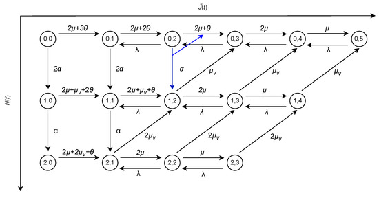
Figure 5. Stochastic lower bounding model. Blue arrows indicate the reassignment of the rate from (0, 2) → (1, 2) to (0, 2) → (0, 3).

5.4. Balance Equations of Stationary Distributions in Irreducible Class $\tilde{\tilde{C}}$

We now derive the global balance equations that characterize the stationary distribution $({\widetilde{\tilde{\mathit{\pi }}}}_1,{\widetilde{\tilde{\mathit{\pi }}}}_2,\dots ,{\widetilde{\tilde{\mathit{\pi }}}}_K)$ over the irreducible class $\tilde{\tilde{C}}$ of the process $\{\tilde{\tilde{X}}(t);t\ge 0\}$.

For i = v and 1 < j^′ ≤ K − v, the global balance equations of ${\tilde{\tilde{\pi }}}_{v,j}$ are given by

$$\begin{array}{c}\hfill \left[\lambda +\sum _{n\in {\tilde{S}}_{j^{\prime }+1}}{({\tilde{\tilde{Q}}}_0^{(j^{\prime })})}_{v,n}\right]{\tilde{\tilde{\pi }}}_{v,j^{\prime }}=\lambda {\tilde{\tilde{\pi }}}_{v,j^{\prime }+1}+{({\tilde{\tilde{Q}}}_0^{(j^{\prime }-1)})}_{v,v}·{\tilde{\tilde{\pi }}}_{v,j^{\prime }-1},1<j^{\prime }<K-v,\end{array}$$

(19)

$$\begin{array}{c}\hfill \left[\lambda +{({\tilde{\tilde{Q}}}_0^{(j^{\prime })})}_{v,v-1}\right]{\tilde{\tilde{\pi }}}_{v,j^{\prime }}={({\tilde{\tilde{Q}}}_0^{(j^{\prime }-1)})}_{v,v}·{\tilde{\tilde{\pi }}}_{v,j^{\prime }-1},j^{\prime }=K-v.\end{array}$$

(20)

For 0 ≤ i ≤ v − 1 and 1 < j^′ ≤ K − i, the global balance equations of ${\tilde{\tilde{\pi }}}_{i,j^{\prime }}$ are given by

$$\begin{array}{cc}\hfill \left[\lambda +\sum _{n\in {\tilde{S}}_{j^{\prime }+1}}{({\tilde{\tilde{Q}}}_0^{(j^{\prime })})}_{i,n}\right]{\tilde{\tilde{\pi }}}_{i,j^{\prime }}& =\lambda {\tilde{\tilde{\pi }}}_{i,j^{\prime }+1}+{({\tilde{\tilde{Q}}}_0^{(j^{\prime }-1)})}_{i,i}·{\tilde{\tilde{\pi }}}_{i,j^{\prime }-1}\hfill \\ & \hspace{1em}+{({\tilde{\tilde{Q}}}_0^{(j^{\prime }-1)})}_{i+1,i}·{\tilde{\tilde{\pi }}}_{i+1,j^{\prime }-1},1<j^{\prime }<K-i,\hfill \end{array}$$

(21)

$$\begin{array}{cc}\hfill \left[\lambda +{({\tilde{\tilde{Q}}}_0^{(j^{\prime })})}_{i,i-1}\right]{\tilde{\tilde{\pi }}}_{i,j^{\prime }}& ={({\tilde{\tilde{Q}}}_0^{(j^{\prime }-1)})}_{i,i}·{\tilde{\tilde{\pi }}}_{i,j^{\prime }-1}\hfill \\ \hfill & \hspace{1em}+{({\tilde{\tilde{Q}}}_0^{(j^{\prime }-1)})}_{i+1,i}·{\tilde{\tilde{\pi }}}_{i+1,j^{\prime }-1},j^{\prime }=K-i.\hfill \end{array}$$

(22)

The global balance equations above do not include expressions for ${\tilde{\tilde{\pi }}}_{i,1}$ with 0 ≤ i ≤ v. To obtain these, we define a subset of the irreducible class as

$$\begin{array}{c}\hfill {\tilde{\tilde{C}}}_i=\{(n,j^{\prime })\mid i\le n\le v,1\le j^{\prime }\le K-i\},0\le i\le v-1,\end{array}$$

and consider the total flow between ${\tilde{\tilde{C}}}_i$ and its complement in $\tilde{\tilde{C}}$. From this, we obtain

$$\begin{array}{c}\hfill (v-i)\alpha {\tilde{\tilde{\pi }}}_{i,1}=\sum _{j^{\prime }=1}^{K-i-1}{({\tilde{\tilde{Q}}}_0^{(j^{\prime })})}_{i+1,i}·{\tilde{\tilde{\pi }}}_{i+1,j^{\prime }},0\le i\le v-1.\end{array}$$

Finally, ${\tilde{\tilde{\pi }}}_{v,1}$ is determined via the normalization condition given by

$$\begin{array}{cc}\hfill \sum _{i=0}^v\sum _{j^{\prime }=1}^{K-i}{\tilde{\tilde{\pi }}}_{i,j^{\prime }}& =1.\hfill \end{array}$$

5.5. Construction of Recurrence Relation

We now construct recurrence relations that determine the stationary probabilities ${\tilde{\tilde{\pi }}}_{v,j^{\prime }}$ for 1 < j^′ ≤ K − v. Observe from the global balance Equation (20) that ${\tilde{\tilde{\pi }}}_{v,K-v}$ is determined if ${\tilde{\tilde{\pi }}}_{v,K-v-1}$ is given. Similarly, from (19) at j^′ = K − v − 1, since ${\tilde{\tilde{\pi }}}_{v,K-v}$ has already been determined from ${\tilde{\tilde{\pi }}}_{v,K-v-1}$, it follows that ${\tilde{\tilde{\pi }}}_{v,K-v-1}$ is determined from ${\tilde{\tilde{\pi }}}_{v,K-v-2}$. Proceeding recursively, for any 1 < j^′ ≤ K − v, ${\tilde{\tilde{\pi }}}_{v,j^{\prime }}$ can be determined from ${\tilde{\tilde{\pi }}}_{v,j^{\prime }-1}$. Therefore, the sequence $\left\{{\tilde{\tilde{\pi }}}_{v,j^{\prime }}\right\}$ is determined by a recurrence relation starting from ${\tilde{\tilde{\pi }}}_{v,1}$. The proof is omitted, as it is analogous to that of Lemma 1.

Lemma 3.

The stationary probability ${\tilde{\tilde{\pi }}}_{v,j^{\prime }}$ for $1<j^{\prime }\le K-v$ satisfies the recurrence relation

$$\begin{array}{c}\hfill {\tilde{\tilde{\pi }}}_{v,j^{\prime }}={\tilde{\tilde{b}}}_{v,j^{\prime }}·{\tilde{\tilde{\pi }}}_{v,j^{\prime }-1},1<j^{\prime }\le K-v,\end{array}$$

where the coefficient ${\tilde{\tilde{b}}}_{v,j^{\prime }}$ is given by

$$\begin{array}{c}\hfill {\tilde{\tilde{b}}}_{v,j^{\prime }}={\displaystyle \frac{{({\tilde{\tilde{Q}}}_0^{(j^{\prime }-1)})}_{v,v}}{\lambda +{({\tilde{\tilde{Q}}}_0^{(j^{\prime })})}_{v,v-1}+{({\tilde{\tilde{Q}}}_0^{(j^{\prime })})}_{v,v}·{\tilde{\tilde{c}}}_{v,j^{\prime }}}},1<j^{\prime }\le K-v,\end{array}$$

and the auxiliary sequence ${\tilde{\tilde{c}}}_{v,j^{\prime }}$ is recursively defined as

$$\begin{array}{cc}\hfill {\tilde{\tilde{c}}}_{v,j^{\prime }}& =\left\{\begin{array}{cc}0,\hfill & j^{\prime }=K-v,\hfill \\ {\displaystyle \frac{{({\tilde{\tilde{Q}}}_0^{(j^{\prime }+1)})}_{v,v-1}+{({\tilde{\tilde{Q}}}_0^{(j^{\prime }+1)})}_{v,v}·{\tilde{\tilde{c}}}_{v,j^{\prime }+1}}{\lambda +{({\tilde{\tilde{Q}}}_0^{(j^{\prime }+1)})}_{v,v-1}+{({\tilde{\tilde{Q}}}_0^{(j^{\prime }+1)})}_{v,v}·{\tilde{\tilde{c}}}_{v,j^{\prime }+1}},}\hfill & 1<j^{\prime }<K-v.\hfill \end{array}\right.\hfill \end{array}$$

Remark 12.

From Lemma 3, we observe that each ${\tilde{\tilde{\pi }}}_{v,j^{\prime }}$ for $1<j^{\prime }\le K-v$ can be recursively expressed in terms of ${\tilde{\tilde{\pi }}}_{v,1}$. Furthermore, consider the balance equation between the subset ${\tilde{\tilde{C}}}_{v-1}$ and its complement $\tilde{\tilde{C}}\setminus {\tilde{\tilde{C}}}_{v-1}$. This equation takes the following form.

$$\begin{array}{c}\hfill \alpha {\tilde{\tilde{\pi }}}_{v-1,1}=\sum _{j^{\prime }=1}^{K-v}{({\tilde{\tilde{Q}}}_0^{(j^{\prime })})}_{v,v-1}·{\tilde{\tilde{\pi }}}_{v,j^{\prime }}.\end{array}$$

Since the right-hand side consists only of terms ${\tilde{\tilde{\pi }}}_{v,j^{\prime }}$ for $1\le j^{\prime }\le K-v$, which in turn can be written in terms of ${\tilde{\tilde{\pi }}}_{v,1}$, it follows that ${\tilde{\tilde{\pi }}}_{v-1,1}$ can also be expressed as a function of ${\tilde{\tilde{\pi }}}_{v,1}$.

Using the global balance Equations (21) and (22), we obtain similar recursive relations as follows. The proof is again omitted, as it is standard and analogous to that of Lemma 2.

Lemma 4.

For $0\le i\le v-1$ and $1<j^{\prime }\le K-i$, the stationary probability ${\tilde{\tilde{\pi }}}_{i,j^{\prime }}$ satisfies the following recurrence relation

$$\begin{array}{c}\hfill {\tilde{\tilde{\pi }}}_{i,j^{\prime }}={\tilde{\tilde{a}}}_{i,j^{\prime }}+{\tilde{\tilde{b}}}_{i,j^{\prime }}·{\tilde{\tilde{\pi }}}_{i,j^{\prime }-1},\end{array}$$

where

$$\begin{array}{cc}\hfill {\tilde{\tilde{a}}}_{i,j^{\prime }}& =\left\{\begin{array}{cc}{\displaystyle \frac{{({\tilde{\tilde{Q}}}_0^{(j^{\prime }-1)})}_{i+1,i}·{\tilde{\tilde{\pi }}}_{i+1,j^{\prime }-1}}{\lambda +{({\tilde{\tilde{Q}}}_0^{(j^{\prime })})}_{i,i-1}},}\hfill & j^{\prime }=K-i,\hfill \\ {\displaystyle \frac{\lambda ·{\tilde{\tilde{a}}}_{i,j^{\prime }+1}+{({\tilde{\tilde{Q}}}_0^{(j^{\prime }-1)})}_{i+1,i}·{\tilde{\tilde{\pi }}}_{i+1,j^{\prime }-1}}{\lambda +{({\tilde{\tilde{Q}}}_0^{(j^{\prime })})}_{i,i-1}+{({\tilde{\tilde{Q}}}_0^{(j^{\prime })})}_{i,i}·{\tilde{\tilde{c}}}_{i,j^{\prime }}},}\hfill & 1<j^{\prime }<K-i,\hfill \end{array}\right.\hfill \\ \hfill {\tilde{\tilde{b}}}_{i,j^{\prime }}& ={\displaystyle \frac{{({\tilde{\tilde{Q}}}_0^{(j^{\prime }-1)})}_{i,i}}{\lambda +{({\tilde{\tilde{Q}}}_0^{(j^{\prime })})}_{i,i-1}+{({\tilde{\tilde{Q}}}_0^{(j^{\prime })})}_{i,i}·{\tilde{\tilde{c}}}_{i,j^{\prime }}}},1<j^{\prime }\le K-i,\hfill \\ \hfill {\tilde{\tilde{c}}}_{i,j^{\prime }}& =\left\{\begin{array}{cc}0,\hfill & j^{\prime }=K-i,\hfill \\ {\displaystyle \frac{{({\tilde{\tilde{Q}}}_0^{(j^{\prime }+1)})}_{i,i-1}+{({\tilde{\tilde{Q}}}_0^{(j^{\prime }+1)})}_{i,i}·{\tilde{\tilde{c}}}_{i,j^{\prime }+1}}{\lambda +{({\tilde{\tilde{Q}}}_0^{(j^{\prime }+1)})}_{i,i-1}+{({\tilde{\tilde{Q}}}_0^{(j^{\prime }+1)})}_{i,i}·{\tilde{\tilde{c}}}_{i,j^{\prime }+1}},}\hfill & 1<j^{\prime }<K-i,\hfill \end{array}\right.\hfill \end{array}$$

with the convention that ${({\tilde{\tilde{Q}}}_0^{(j^{\prime }+1)})}_{0,-1}=0$ for $1<j^{\prime }\le K$.

Remark 13.

From Lemma 4, it follows that the sequence ${\tilde{\tilde{\pi }}}_{v-1,j^{\prime }}$ for $1<j^{\prime }\le K-v+1$ can be expressed in terms of ${\tilde{\tilde{\pi }}}_{v-1,1}$ and ${\tilde{\tilde{\pi }}}_{v,j^{\prime }}$ for $1\le j^{\prime }\le K-v$. In addition, consider the balance equation between ${\tilde{\tilde{C}}}_{v-2}$ and its complement $\tilde{\tilde{C}}\setminus {\tilde{\tilde{C}}}_{v-2}$ obtained as

$$\begin{array}{c}\hfill 2\alpha {\tilde{\tilde{\pi }}}_{v-2,1}=\sum _{j^{\prime }=1}^{K-v+1}{({\tilde{\tilde{Q}}}_0^{(j^{\prime })})}_{v-1,v-2}·{\tilde{\tilde{\pi }}}_{v-1,j^{\prime }}.\end{array}$$

The right-hand side depends only on ${\tilde{\tilde{\pi }}}_{v-1,j^{\prime }}$ for $1<j^{\prime }\le K-v+1$, and thus ${\tilde{\tilde{\pi }}}_{v-2,1}$ can be written in terms of ${\tilde{\tilde{\pi }}}_{v-1,1}$. Furthermore, from Lemma 3, ${\tilde{\tilde{\pi }}}_{v-1,1}$ and ${\tilde{\tilde{\pi }}}_{v,j^{\prime }}$ (for $1<j^{\prime }\le K-v$) are also expressed in terms of ${\tilde{\tilde{\pi }}}_{v,1}$. Hence, ${\tilde{\tilde{\pi }}}_{v-2,1}$ and all ${\tilde{\tilde{\pi }}}_{v-1,j^{\prime }}$ (for $1<j^{\prime }\le K-v+1$) can be expressed in terms of ${\tilde{\tilde{\pi }}}_{v,1}$.

By iterating this argument for $i=v-3,v-4,\dots ,0$, using the balance equations between ${\tilde{\tilde{C}}}_i$ and $\tilde{\tilde{C}}\setminus {\tilde{\tilde{C}}}_i$, and applying Lemma 4 repeatedly, we conclude that all ${\tilde{\tilde{\pi }}}_{i,j^{\prime }}$ for $0\le i\le v-1$ and $1\le j^{\prime }\le K-i$ can ultimately be expressed in terms of ${\tilde{\tilde{\pi }}}_{v,1}$.

6. Bounds of Performance Metrics

This section presents bounds for key performance metrics. It is important to note that the partial order relations underlying the stochastic comparison are defined with respect to the level variables of the LDQBD processes, but the definitions of the level variables differ between the upper and lower bounding models. In the upper bounding model, the level variable is defined as the sum of the number of jobs being processed by the legacy servers and the number of jobs waiting in the queue. Accordingly, the resulting performance bounds pertain to the number of waiting jobs. In contrast, in the lower bounding model, the level variable represents the total number of jobs in the system, including both jobs in waiting and those in service. Thus, the bounds derived from the lower model are based on the total number of jobs in system.

6.1. Upper Bound of Performance Metrics

Let L_q denote the expected number of jobs waiting in the queue in the original model, whose stationary distribution is denoted by π. Let $L_q^u$ denote the corresponding expectation in the upper bounding model with stationary distribution $\check{\mathit{\pi }}$. Define a monotone function $f:\widehat{S}\to \mathbb{R}$ by

$$\begin{array}{cc}\hfill f((i,j))& ={[j-l]}^{+},\mathrm{for}(i,j)\in \widehat{S}.\hfill \end{array}$$

Since $\widehat{\mathit{\pi }}$ and π have the same support and satisfy $\widehat{\mathit{\pi }}{\le }_s\check{\mathit{\pi }}$, we obtain the following inequality:

$$\begin{array}{cc}\hfill L_q& =\sum _{j=0}^K{[j-l]}^{+}{\mathit{\pi }}_j\mathbf{1}=\sum _{j=0}^K{[j-l]}^{+}{\widehat{\mathit{\pi }}}_j\mathbf{1}\hfill \\ \hfill & =\sum _{j=0}^{K+1}{[j-l]}^{+}{\widehat{\mathit{\pi }}}_j\mathbf{1}\le \sum _{j=0}^{K+1}{[j-l]}^{+}{\check{\mathit{\pi }}}_j\mathbf{1}=L_q^u.\hfill \end{array}$$

Note that ${\widehat{\mathit{\pi }}}_{K+1}$ is the zero vector, and thus the sum over j = 0 to K + 1 does not affect the total value.

Let W_q and P_B denote the expected waiting time and the loss probability of a job in the original model with stationary distribution π, respectively. By applying Little’s law, we obtain the following relation:

$$\begin{array}{cc}\hfill W_q& ={\displaystyle \frac{L_q}{\lambda (1-P_B)}}\le {\displaystyle \frac{L_q^u}{\lambda (1-P_B^u)}},\hfill \end{array}$$

where $P_B^u$ is any non-negative constant satisfying $P_B\le P_B^u<1$. It should be emphasized that although P_B can be expressed as

$$\begin{array}{cc}\hfill P_B& =\sum _{i+j=K,(i,j)\in \widehat{S}}{\pi }_{i,j}=\sum _{i+j=K,(i,j)\in \widehat{S}}{\widehat{\pi }}_{i,j},\hfill \end{array}$$

we cannot guarantee the inequality

$$\begin{array}{cc}\hfill \sum _{i+j=K,(i,j)\in \widehat{S}}{\widehat{\pi }}_{i,j}& \le \sum _{i+j=K,(i,j)\in \widehat{S}}{\check{\pi }}_{i,j}.\hfill \end{array}$$

In our stochastic dominance framework, performance metrics can be compared when they can be represented as expectations of monotone functions. Since the loss rate P_B cannot be expressed as a monotone function with respect to the chosen partial order, it cannot be bounded above using the upper bounding distribution $\check{\mathit{\pi }}$, and hence $P_B^u$ cannot be chosen as ${\sum }_{i+j=K,(i,j)\in \widehat{S}}{\check{\pi }}_{i,j}$. As a result, in order to evaluate an upper bound on W_q, it is necessary to use an external estimate $P_B^u$ satisfying $P_B\le P_B^u<1$.

To obtain $P_B^u$ which is easy to calculate and still holds the relation $P_B\le P_B^u<1$, we consider the LDQBD process $\{\tilde{X}(t);t\ge 0\}$ with the level variable as the number of jobs in the system with the stationary distribution $\tilde{\mathit{\pi }}=({\tilde{\mathit{\pi }}}_0,{\tilde{\mathit{\pi }}}_1,\dots ,{\tilde{\mathit{\pi }}}_K)$. According to [8], the probability distribution ${\left\{{\ell }_j\right\}}_{0\le j\le K}$ that satisfies ${\sum }_{j=k}^K{\tilde{\mathit{\pi }}}_j\mathbf{1}\le {\sum }_{j=k}^K{\ell }_j$ for any $k(0\le k\le K)$ is given by

$$\begin{array}{c}{\ell }_0=0,{\ell }_1={\left[1+\sum _{j=2}^K\prod _{k=1}^{j-1}{\displaystyle \frac{\lambda }{{\mu }_{k+1,k}}}\right]}^{-1},{\ell }_j={\ell }_1\prod _{k=1}^{j-1}{\displaystyle \frac{\lambda }{{\mu }_{k+1,k}}},2\le j\le K,\end{array}$$

where

$$\begin{array}{cc}\hfill {\mu }_{j+1,j}& =min\{(l\wedge j)\mu +(0\wedge j){\mu }_v+{[j-l]}^{+}\theta ,\dots ,(l\wedge j)\mu +(v\wedge j){\mu }_v+{[j-v-l]}^{+}\theta \}\hfill \end{array}$$

for 1 ≤ j ≤ K. Since $P_B={\tilde{\mathit{\pi }}}_K\mathbf{1}$ by the PASTA (Poisson Arrivals See Time Averages) property [24], we can choose $P_B^u$ such that $P_B\le P_B^u<1$ by letting $P_B^u={\ell }_K$. Therefore, W_q is bounded by $W_q^u$ which is given by

$$\begin{array}{cc}\hfill W_q^u& ={\displaystyle \frac{L_q^u}{\lambda (1-{\ell }_K)}}.\hfill \end{array}$$

Let W denote the expected sojourn time in the original system, i.e., the expected total time a job spends in the system. Then, we have

$$\begin{array}{cc}\hfill W& =W_q+{\mu }^{-1}{s}_l+{\mu }_v^{-1}{s}_v,\hfill \end{array}$$

where s_l is the probability that a job does not abandon the queue and is served by a legacy server, and s_v is the probability that a job does not abandon the queue and is served by a virtual server. Since s_l ≤ 1 and s_v ≤ 1, we obtain the following upper bound:

$$\begin{array}{cc}\hfill W& \le W_q+max\{{\mu }^{-1},{\mu }_v^{-1}\}.\hfill \end{array}$$

Therefore, by using the previously obtained bound $W_q\le W_q^u$, we obtain the upper bound W^u for W as

$$\begin{array}{cc}\hfill W^u& =W_q^u+max\{{\mu }^{-1},{\mu }_v^{-1}\}.\hfill \end{array}$$

6.2. Lower Bound of Performance Metrics

Let us choose a monotone function f on $\tilde{S}$ defined by f((i, j^′)) = j^′ for $(i,j^{\prime })\in \tilde{S}$. Since $\tilde{\mathit{\pi }}{\le }_s\widetilde{\tilde{\mathit{\pi }}}$, the following inequality holds:

$$\begin{array}{c}\hfill \sum _{j^{\prime }=0}^K{j}^{\prime }{\tilde{\mathit{\pi }}}_{j^{\prime }}\mathbf{1}\le \sum _{j^{\prime }=0}^K{j}^{\prime }{\widetilde{\tilde{\mathit{\pi }}}}_{j^{\prime }}\mathbf{1}.\end{array}$$

Let L denote the expected number of jobs in the system in the original model with stationary distribution $\tilde{\mathit{\pi }}$, and let L^l denote that of the lower bounding model with stationary distribution $\widetilde{\tilde{\mathit{\pi }}}$. Since the level variable ${\tilde{J}}^{\prime }(t)$ of the process $\{\tilde{X}(t)=(\tilde{N}(t),{\tilde{J}}^{\prime }(t));t\ge 0\}$ is related to the actual number of jobs $\tilde{J}(t)$ by ${\tilde{J}}^{\prime }(t)=K-\tilde{J}(t)$, we have

$$\begin{array}{c}\hfill L=\sum _{j=0}^{K}j{\tilde{\mathit{\pi }}}_{K-j}\mathbf{1}=\sum _{j^{\prime }=0}^K(K-j^{\prime }){\tilde{\mathit{\pi }}}_{j^{\prime }}\mathbf{1}\ge \sum _{j^{\prime }=0}^K(K-j^{\prime }){\widetilde{\tilde{\mathit{\pi }}}}_{j^{\prime }}\mathbf{1}=\sum _{j=0}^{K}j{\widetilde{\tilde{\mathit{\pi }}}}_{K-j}\mathbf{1}=L^l.\end{array}$$

Next, let P_B and $P_B^l$ denote the job loss rates in the original and lower bounding models, respectively. Since $P_B={\tilde{\mathit{\pi }}}_0\mathbf{1}\ge {\widetilde{\tilde{\mathit{\pi }}}}_0\mathbf{1}=P_B^l$ and the probability masses of ${\widetilde{\tilde{\mathit{\pi }}}}_0$ are all zero, we have $P_B^l=0$. Therefore,

$$\begin{array}{c}\hfill W={\displaystyle \frac{L}{\lambda (1-P_B)}}\ge {\displaystyle \frac{L^l}{\lambda (1-P_B^l)}}={\displaystyle \frac{L^l}{\lambda }}=W^l,\end{array}$$

which gives a lower bound for the expected sojourn time.

7. Numerical Results

In this section, we present numerical results based on the stationary distribution of the LDQBD process. Specifically, we provide two types of validation: (i) a comparison between the numerical results and the upper bounding models given in Proposition 1 and Theorem 1 and (ii) a comparison between the upper and lower bounds established in Theorems 1 and 2.

7.1. Comparison of Upper Bounding Models

Table 2 compares the marginal tail probabilities ${\sum }_{j=k}^K{\mathit{\pi }}_j\mathbf{1}$, ${\sum }_{j=k}^{K+1}{\overline{\mathit{\pi }}}_j\mathbf{1}$, and ${\sum }_{j=k}^{K+1}{\check{\mathit{\pi }}}_j\mathbf{1}$, obtained from the original model, Proposition 1, and Theorem 1, respectively. We consider two values of the parameter λ, namely λ = 1 and λ = 10, while fixing the remaining parameters at l = 10, v = 20, K = 35, μ = 1, μ_v = 2, α = 0.01, and θ = 1. We observe that the marginal tail probabilities obtained from Proposition 1 and Theorem 1 are larger than those of the original model, as expected. However, Theorem 1 provides a tighter upper bound than Proposition 1 for the original model under these parameter settings.

Table 2. Marginal tail probabilities for the original model, Proposition 1, and Theorem 1.

	k	5	10	15	20
λ = 1	Original Model	3.66 × 10−3	1.11 × 10−7	2.97 × 10−13	1.53 × 10−19
	Proposition 1	1.00 × 100	1.00 × 100	1.00 × 100	9.76 × 10−1
	Theorem 1	1.90 × 10−2	1.20 × 10−6	6.81 × 10−12	4.70 × 10−18
λ = 10	Original Model	9.71 × 10−1	5.38 × 10−1	8.05 × 10−2	3.20 × 10−3
	Proposition 1	1.00 × 100	1.00 × 100	1.00 × 100	1.00 × 100
	Theorem 1	1.00 × 100	9.91 × 10−1	2.35 × 10−1	1.22 × 10−2

Figure 6 shows a comparison of the expected waiting time obtained from the upper bounding models, as well as from the original model, as the value of μ_v varies. Figure 6a and Figure 6b correspond to the cases where λ = 1 and λ = 10, respectively. The other parameters are fixed at l = 10, v = 20, K = 35, μ = 1, α = 0.01, and θ = 1.

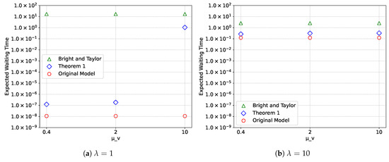
Figure 6. Expected waiting time for various values of μ_v.

Similarly, Figure 7 shows a comparison of the expected waiting time from the upper bounding models, along with the original model, as the value of α varies. Again, Figure 7a and Figure 7b correspond to λ = 1 and λ = 10, respectively. The remaining parameters are set to l = 10, v = 20, K = 35, μ = 1, μ_v = 2, and θ = 1.

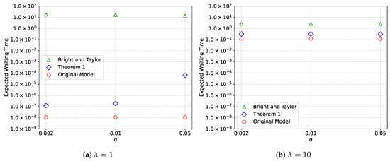
Figure 7. Expected waiting time for various values of α.

These figures show that the upper bounding model proposed in Theorem 1 provides a significantly tighter approximation than the one in Proposition 1, originally developed by Bright and Taylor [8], across a wide range of system parameters.

As shown in Example 1, the transition rate matrix ${\overline{Q}}_0^{(k)}$ given by Proposition 1 is fully populated with nonzero entries related to λ, whereas ${\widehat{Q}}_0^{(k)}$ is not. In contrast, ${\check{Q}}_0^{(j)}$ as defined in Theorem 1 preserves zeros in the same positions as ${\widehat{Q}}_0^{(k)}$. This difference likely accounts for the significant discrepancy between Proposition 1 and Theorem 1 regarding the upper bound of the expected waiting time at λ = 1. It is also worth noting that the expected waiting time based on Theorem 1 can be computed from the stationary distribution obtained via recurrence relations. This implies that one can estimate performance metrics with high accuracy while avoiding expensive computational costs.

7.2. Upper and Lower Bounding Models

Figure 8 shows a comparison of the expected sojourn time obtained from the upper and lower bounding models, as well as from the original model, for various values of μ_v. Figure 8a and Figure 8b correspond to the cases where λ = 1 and λ = 10, respectively. The other parameters are fixed at l = 10, v = 20, K = 35, μ = 1, α = 0.01, and θ = 1.

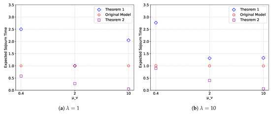
Figure 8. Expected sojourn time for various values of μ_v.

Similarly, Figure 9 presents a comparison of the expected sojourn time obtained from the upper and lower bounding models, along with the original model, for various values of α. Again, Figure 9a and Figure 9b correspond to λ = 1 and λ = 10, respectively. The remaining parameters are set to l = 10, v = 20, K = 35, μ = 1, μ_v = 2, and θ = 1.

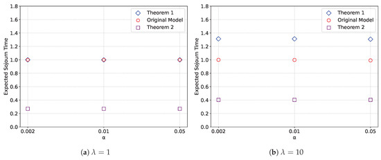
Figure 9. Expected sojourn time for various values of α.

We observe that the accuracy of the upper bound for the expected sojourn time depends on the value of μ_v, which may be due to the term $max{\mu }^{-1},{\mu }_v^{-1}$ in W^u. In contrast, the accuracy of the lower bound deteriorates monotonically as μ_v increases.

Regarding the dependence on the setup rate α of virtual servers, both the upper and lower bounds for the expected sojourn time appear to be almost insensitive to changes in α, indicating that the range between the bounds is robust with respect to α. Overall, the upper bound provides a more accurate estimate of the expected sojourn time than the lower bound.

7.3. CPU Time

We demonstrate performance improvements achieved by the proposed recurrence-based method. As the performance metric, we use the CPU time required to obtain the upper bound of the expected waiting time. Both the matrix analytic method and our recurrence-based method were implemented in MATLAB^® R2025a. Experiments were conducted on a laptop with a 2.4 GHz quad-core CPU and 16 GB of main memory. For each method, CPU times were measured over 10 independent runs.

Table 3 compares the CPU times required to obtain the upper bound of the expected waiting time, based on the stationary distribution in Theorem 1, between the direct application of the matrix analytic method and the proposed recurrence-based method. The parameter v was varied from 1000 to 1500 in increments of 100. The other parameters were fixed at λ = 40, l = 10, μ = 1, α = 0.05, θ = 1, and μ_v = 2. Note that K = l + v = 10 + v, and thus K also varies with v.

Table 3. Maximum, average, and minimum CPU times (in seconds) required to obtain the upper bound of the expected waiting time. “N/A” indicates that the computation could not be completed due to insufficient memory.

		v
		1000	1100	1200	1300	1400	1500
Matrix analytic method	maximum	236.4	330.1	431.3	N/A	N/A	N/A
	average	230.1	319.6	419.8	N/A	N/A	N/A
	minimum	217.3	297.4	399.4	N/A	N/A	N/A
Recurrence-based method	maximum	102.0	144.4	187.2	247.9	311.0	439.9
	average	98.7	138.6	181.6	239.5	305.0	416.2
	minimum	96.2	134.9	178.4	230.9	298.8	406.6

We observe that the proposed recurrence-based method outperforms the matrix analytic method in terms of CPU time for v = 1000, 1100, and 1200. For v greater than 1200, the matrix analytic method fails to compute the upper bound of the expected waiting time in our computing environment due to insufficient memory. In contrast, the recurrence-based method successfully computes the upper bound in all cases. It is also noteworthy that the CPU time of the recurrence-based method at v = 1500 is almost comparable to that of the matrix analytic method at v = 1200.

8. Conclusions

In this paper, we analyzed the queueing model of hybrid systems proposed by Sato et al. [1], formulated as an LDQBD process. By exploiting the structural properties of the transition rates specific to this model and refining the bounding technique developed by Bright and Taylor [8], we derived both upper and lower stochastic bounds for the stationary distribution, which can be efficiently computed using recurrence relations.

Thanks to these recurrence relations, the upper and lower bounds can be obtained with a significant reduction in computational cost. Furthermore, we showed that key performance metrics computed from the true stationary distribution are bounded above and below by our proposed stochastic bounds. We also conducted numerical experiments to evaluate the sensitivity of these performance metrics to variations in system parameters.

The derivation of the bounds relies heavily on the specific structural properties of the transition rates in the LDQBD process of the queueing model. Extending the applicability of our approach to more general LDQBD processes remains an important topic for future research. Another key challenge is to establish error bounds on the difference between the bounding and the true stationary distributions, which we leave for future work.

Appendix A.1. Block Matrices of Q

The block matrices $Q_0^{(j)}$ for 0 ≤ j < l, $Q_1^{(j)}$ for 0 ≤ j ≤ l, and $Q_2^{(j)}$ for 0 < j ≤ l are (v + 1) × (v + 1) matrices given by

$$\begin{array}{cc}\hfill Q_0^{(j)}=\lambda I,& Q_1^{(j)}=\left[\begin{array}{ccccc}-q_{0,j}& 0& \dots & \dots & 0\\ {\mu }_v& -q_{1,j}& \ddots & & ⋮\\ ⋮& 2{\mu }_v& \ddots & \ddots & ⋮\\ ⋮& & \ddots & \ddots & 0\\ 0& \dots & \dots & v{\mu }_v& -q_{v,j}\end{array}\right],Q_2^{(j)}=j\mu I,\hfill \end{array}$$

where I is the identity matrix of appropriate size. The exit rate q_i,j of state (i, j) ∈ S for 0 ≤ i ≤ v and 0 ≤ j ≤ l is given by

$$\begin{array}{cc}\hfill q_{i,j}& =\lambda +j\mu +i{\mu }_v.\hfill \end{array}$$

The matrices $Q_0^{(j)}$ for l ≤ j < l + v, $Q_1^{(j)}$ for l < j ≤ l + v, and $Q_2^{(j)}$ for l < j ≤ l + v are (v + 1) × (v + 1) matrices given by

$$\begin{array}{cc}\hfill Q_0^{(j)}& =\lambda I,Q_1^{(j)}=-\mathrm{diag}\{q_{0,j},q_{1,j},\dots ,q_{v,j}\},\hfill \\ \hfill Q_2^{(j)}& =\left\{l\mu +(j-l)\theta \right\}I+{\mu }_v\mathrm{diag}\{0,1,\dots ,v\}\hfill \\ \hfill & +\left[\begin{array}{ccccc}0& p_{0,j}\alpha & 0& \dots & 0\\ 0& \ddots & p_{1,j}\alpha & \ddots & ⋮\\ ⋮& \ddots & \ddots & \ddots & 0\\ ⋮& & \ddots & \ddots & p_{v-1,j}\alpha \\ 0& \dots & \dots & 0& 0\end{array}\right],\hfill \end{array}$$

where p_i,j = (j − l) ∧ (v − i). The exit rate q_i,j of state (i, j) ∈ S, for 0 ≤ i ≤ v and l < j ≤ l + v, is given by

$$\begin{array}{cc}\hfill q_{i,j}& =\lambda +l\mu +(j-l)\theta +i{\mu }_v+p_{i,j}\alpha .\hfill \end{array}$$

The matrices $Q_0^{(j)}$ for l + v ≤ j < K, $Q_1^{(j)}$ for l + v < j ≤ K, and $Q_2^{(j)}$ for l + v < j ≤ K are (K − j + 1) × (K − j), (K − j + 1) × (K − j + 1), and (K − j + 1) × (K − j + 2) matrices, respectively, and are explicitly given by

$$\begin{array}{cc}\hfill Q_0^{(j)}& =\left[\begin{array}{}\begin{array}{cccc}\lambda & 0& \dots & 0\\ 0& \lambda & \ddots & ⋮\\ ⋮& \ddots & \ddots & 0\\ 0& \dots & 0& \lambda \end{array}\\ \begin{array}{c}\mathbf{0}\end{array}\end{array}\right],Q_1^{(j)}=-\mathrm{diag}\{q_{0,j},q_{1,j},\dots ,q_{K-j,j}\},\hfill \\ \hfill Q_2^{(j)}& =\left[\begin{array}{cc}\{l\mu +(j-l)\theta \}I& {\mathbf{0}}^{\top }\end{array}\right]+\left[\begin{array}{cc}{\mu }_v\mathrm{diag}\{0,1,\dots ,v\}& {\mathbf{0}}^{\top }\end{array}\right]\hfill \\ \hfill & +\left[\begin{array}{ccccc}0& p_{0,j}\alpha & 0& \dots & 0\\ ⋮& \ddots & p_{1,j}\alpha & \ddots & ⋮\\ ⋮& & \ddots & \ddots & 0\\ 0& \dots & \dots & 0& p_{K-j,j}\alpha \end{array}\right],\hfill \end{array}$$

where 0^⊤ denotes the column vector of all zeros, i.e., the transpose of the row vector 0 defined in the main text. The exit rate q_i,j of state (i, j) ∈ S, for 0 ≤ i ≤ K − j and l + v < j ≤ K, is given by

$$\begin{array}{cc}\hfill q_{i,j}& =\left\{\begin{array}{cc}\lambda +l\mu +(j-l)\theta +i{\mu }_v+p_{i,j}\alpha ,\hfill & j\ne K,\hfill \\ l\mu +(j-l)\theta +i{\mu }_v+p_{i,j}\alpha ,\hfill & j=K.\hfill \end{array}\right.\hfill \end{array}$$

Appendix A.2. Block Matrices of $\tilde{Q}$

The block matrices ${\tilde{Q}}_0^{(j^{\prime })}$ for 0 ≤ j^′ < K − l − v, ${\tilde{Q}}_1^{(j^{\prime })}$ for 0 ≤ j^′ < K − l − v, and ${\tilde{Q}}_2^{(j^{\prime })}$ for 0 < j^′ ≤ K − l − v are (v + 1) × (v + 1) matrices given by

$$\begin{array}{cc}\hfill {\tilde{Q}}_0^{(j^{\prime })}& =l\mu I+{\mu }_v\mathrm{diag}\{0,1,\dots ,v\}+\theta \mathrm{diag}\{K-l-j^{\prime },K-l-1-j^{\prime },\dots ,K-l-v-j^{\prime }\},\hfill \\ \hfill {\tilde{Q}}_1^{(j^{\prime })}& =\left[\begin{array}{ccccc}-{\tilde{q}}_{0,j^{\prime }}& v\alpha & 0& \dots & 0\\ 0& -{\tilde{q}}_{1,j^{\prime }}& (v-1)\alpha & \ddots & ⋮\\ ⋮& \ddots & \ddots & \ddots & 0\\ ⋮& & \ddots & \ddots & \alpha \\ 0& \dots & \dots & 0& -{\tilde{q}}_{v,j^{\prime }}\end{array}\right],{\tilde{Q}}_2^{(j^{\prime })}=\lambda I,\hfill \end{array}$$

where ${\tilde{q}}_{i,j^{\prime }}$ for state $(i,j^{\prime })\in \tilde{S}$ with 0 ≤ i ≤ v and 0 ≤ j^′ < K − l − v is given by

$$\begin{array}{cc}\hfill {\tilde{q}}_{i,j^{\prime }}& =\left\{\begin{array}{cc}l\mu +(K-l-i)\theta +i{\mu }_v+(v-i)\alpha ,\hfill & j^{\prime }=0,\hfill \\ \lambda +l\mu +(K-l-i-j^{\prime })\theta +i{\mu }_v+(v-i)\alpha ,\hfill & j^{\prime }\ne 0.\hfill \end{array}\right.\hfill \end{array}$$

The matrices ${\tilde{Q}}_0^{(j^{\prime })}$ for K − l − v ≤ j^′ < K − l, ${\tilde{Q}}_1^{(j^{\prime })}$ for K − l − v ≤ j^′ < K − l, and ${\tilde{Q}}_2^{(j^{\prime })}$ for K − l − v < j^′ ≤ K − l are (v + 1) × (v + 1) matrices given by

$$\begin{array}{cc}\hfill {\tilde{Q}}_0^{(j^{\prime })}& =\mu \mathrm{diag}\left\{l\wedge (K-j^{\prime }),l\wedge (K-j^{\prime }-1),\dots ,l\wedge (K-j^{\prime }-v)\right\}\hfill \\ \hfill & +\theta \mathrm{diag}\left\{{[K-j^{\prime }-l]}^{+},{[K-j^{\prime }-l-1]}^{+},\dots ,{[K-j^{\prime }-l-v]}^{+}\right\}\hfill \\ \hfill & +{\mu }_v\left[\begin{array}{ccccc}{\tilde{r}}_{0,j^{\prime }}& 0& \dots & \dots & 0\\ 1-{\tilde{r}}_{1,j^{\prime }}& {\tilde{r}}_{1,j^{\prime }}& \ddots & & ⋮\\ 0& \ddots & \ddots & \ddots & ⋮\\ ⋮& \ddots & \ddots & \ddots & 0\\ 0& \dots & 0& v-{\tilde{r}}_{v,j^{\prime }}& {\tilde{r}}_{v,j^{\prime }}\end{array}\right],\hfill \\ \hfill {\tilde{Q}}_1^{(j^{\prime })}& =\left[\begin{array}{ccccc}-{\tilde{q}}_{0,j^{\prime }}& \alpha {\tilde{p}}_{0,j^{\prime }}& 0& \dots & 0\\ 0& -{\tilde{q}}_{1,j^{\prime }}& \alpha {\tilde{p}}_{1,j^{\prime }}& \ddots & ⋮\\ ⋮& \ddots & \ddots & \ddots & 0\\ ⋮& & \ddots & \ddots & \alpha {\tilde{p}}_{v-1,j^{\prime }}\\ 0& \dots & \dots & 0& -{\tilde{q}}_{v,j^{\prime }}\end{array}\right],{\tilde{Q}}_2^{(j^{\prime })}=\lambda I,\hfill \end{array}$$

where ${\tilde{r}}_{i,j^{\prime }}=i$ if i < K − j^′ − l, and ${\tilde{r}}_{i,j^{\prime }}=0$ otherwise, and ${\tilde{p}}_{i,j^{\prime }}=v\wedge {[K-j^{\prime }-l-i]}^{+}$. The exit rate ${\tilde{q}}_{i,j^{\prime }}$ of state $(i,j^{\prime })\in \tilde{S}$ for 0 ≤ i ≤ v and K − l − v ≤ j^′ < K − l is given by

$$\begin{array}{cc}\hfill {\tilde{q}}_{i,j^{\prime }}& =\lambda +(l\wedge (K-j^{\prime }-i))\mu +{[K-j^{\prime }-l-i]}^{+}\theta +i{\mu }_v+{\tilde{p}}_{i,j^{\prime }}\alpha .\hfill \end{array}$$

The matrices ${\tilde{Q}}_0^{(j^{\prime })}$ for K − l ≤ j^′ < K, ${\tilde{Q}}_1^{(j^{\prime })}$ for K − l ≤ j^′ ≤ K, and ${\tilde{Q}}_2^{(j^{\prime })}$ for K − l < j^′ ≤ K are (K − j^′ + 1) × (K − j^′), (K − j^′ + 1) × (K − j^′ + 1), and (K − j^′ + 1) × (K − j^′ + 2) matrices, respectively, and are explicitly given by

$$\begin{array}{cc}\hfill {\tilde{Q}}_0^{(j^{\prime })}& =\left[\begin{array}{cccc}(l\wedge (K-j^{\prime }))\mu & 0& \dots & 0\\ {\mu }_v& (l\wedge (K-j^{\prime }-1))\mu & \ddots & ⋮\\ 0& 2{\mu }_v& \ddots & 0\\ ⋮& \ddots & \ddots & (l\wedge 1)\mu \\ 0& \dots & 0& (K-j^{\prime }){\mu }_v\end{array}\right],\hspace{1em}\hfill \\ \hfill {\tilde{Q}}_1^{(j^{\prime })}& =-\mathrm{diag}\{{\tilde{q}}_{0,j^{\prime }},{\tilde{q}}_{1,j^{\prime }},\dots ,{\tilde{q}}_{K-j^{\prime },j^{\prime }}\},{\tilde{Q}}_2^{(j^{\prime })}=\left[\begin{array}{cc}\lambda I& {\mathbf{0}}^{\top }\end{array}\right],\hfill \end{array}$$

where the exit rate ${\tilde{q}}_{i,j^{\prime }}$ of state $(i,j^{\prime })\in \tilde{S}$ for 0 ≤ i ≤ K − j^′ and K − l ≤ j^′ ≤ K is given by

$$\begin{array}{cc}\hfill {\tilde{q}}_{i,j^{\prime }}& =\left\{\begin{array}{cc}\lambda +(l\wedge (K-j^{\prime }-i))\mu +i{\mu }_v,\hfill & j^{\prime }\ne K,\hfill \\ \lambda ,\hfill & j^{\prime }=K.\hfill \end{array}\right.\hfill \end{array}$$

Appendix B.1. Preliminaries

Let S be a set equipped with a partial order relation ⪯. A subset Γ ⊂ S is called an increasing set if it satisfies the following condition.

$$\begin{array}{c}\hfill x\in \Gamma ,x⪯y\Rightarrow y\in \Gamma .\end{array}$$

We prove Theorems 1 and 2 using the following lemma, established by Massey [25] for uniform Markov processes and later extended by Brandt and Last [26] to accommodate non-uniform Markov processes.

Lemma A1.

Let $q_1$ and $q_2$ be Markov processes on a common state space S, equipped with a partial order ⪯ . Suppose that for all $x,y\in S$ such that $x⪯y$, and for all increasing sets $\Gamma \subset S$, the following two conditions hold.

(i)

If $x,y\in \Gamma$, then

$$\sum _{z\notin \Gamma }{q}_1(x,z)\ge \sum _{z\notin \Gamma }{q}_2(y,z).$$

(ii)

If $x,y\notin \Gamma$, then

$$\sum _{z\in \Gamma }{q}_1(x,z)\le \sum _{z\in \Gamma }{q}_2(y,z).$$

Then, $q_2$ stochastically dominates $q_1$ with respect to the partial order ⪯.

Let $\mathcal{P}$(M) denote the power set of a set M. Following the idea of [8], we define a family of increasing sets for the LDQBD processes on $\widehat{S}$ in the following form.

$$\begin{array}{c}\hfill {\Phi }_{I,j}=I\cup \left(\bigcup _{k=j}^{\infty }{\widehat{S}}_k\right),I\in \mathcal{P}({\widehat{S}}_{j-1}),I\ne \varnothing ,j\ge 1.\end{array}$$

Note that the family

$$\begin{array}{c}\hfill {\mathcal{I}}_j=\left\{{\Phi }_{I,j}|I\in \mathcal{P}({\widehat{S}}_{j-1}),I\ne \varnothing \right\},j\ge 1\end{array}$$

satisfies the following property:

$$\begin{array}{c}\hfill {\mathcal{I}}_j\cap {\mathcal{I}}_k=\varnothing \mathrm{for}j\ne k.\end{array}$$

Similarly, for the LDQBD processes on $\tilde{S}$, we define increasing sets as

$$\begin{array}{c}\hfill {\Phi }_{I^{\prime },j^{\prime }}^{\prime }=I^{\prime }\cup \left(\bigcup _{k=j^{\prime }}^K{\tilde{S}}_k\right),I^{\prime }\in \mathcal{P}({\tilde{S}}_{j^{\prime }-1}),I^{\prime }\ne \varnothing ,1\le j^{\prime }\le K,\end{array}$$

and define

$$\begin{array}{c}\hfill {\mathcal{I}}_{j^{\prime }}^{\prime }=\left\{{\Phi }_{I^{\prime },j^{\prime }}^{\prime }|I^{\prime }\in \mathcal{P}({\tilde{S}}_{j^{\prime }-1}),I^{\prime }\ne \varnothing \right\},1\le j^{\prime }\le K,\end{array}$$

which also satisfies the following property.

$$\begin{array}{c}\hfill {\mathcal{I}}_{j^{\prime }}^{\prime }\cap {\mathcal{I}}_{k^{\prime }}^{\prime }=\varnothing \mathrm{for}{j}^{\prime }\ne k^{\prime }.\end{array}$$

Appendix B.2. Proof of Theorem 1

For the proof of Theorem 1, we apply Lemma A1 to LDQBD processes defined on the state space $\widehat{S}$, equipped with the partial order ⪯ as defined in Definition 2. We associate q₁ in Lemma A1 with the generator of $\{\widehat{X}(t);t\ge 0\}$ and q₂ with that of $\{\check{X}(t);t\ge 0\}$. We then verify that the two sufficient conditions (i) and (ii) in Lemma A1 are satisfied for every pair of states $x,y\in \widehat{S}$ such that x ⪯ y and for every increasing set $\Gamma \subset \widehat{S}$ of the form Φ_I,j defined in the previous subsection.

Before presenting the detailed proof, we outline its structure. The proof is divided into two parts, corresponding to the two sufficient conditions (i) and (ii) in Lemma A1. For each condition, we examine all non-trivial relevant cases for every pair of states $x,y\in \widehat{S}$ satisfying x ⪯ y and for every increasing set $\Gamma \subset \widehat{S}$ of the form Φ_I,j.

Proof. 

• Verification of condition $(\mathrm{i})$

We verify condition $(\mathrm{i})$ in Lemma A1.

• In the case of $x\prec y\in \Gamma$

  –

  For $\Gamma \in {\mathcal{I}}_j$, $j>1$, we may choose $x=(i,j-1)$ and $y=(k,j)$. Then, it holds that

  $$\begin{array}{cc}\hfill \sum _{z\notin \Gamma }{q}_1(x,z)& =\sum _{n:(n,j-1)\notin \Gamma }{({\widehat{Q}}_1^{(j-1)})}_{i,n}+\sum _{n:(n,j-2)\notin \Gamma }{({\widehat{Q}}_2^{(j-1)})}_{i,n},\hfill \\ \hfill \sum _{z\notin \Gamma }{q}_2(y,z)& =\sum _{n:(n,j-1)\notin \Gamma }{({\check{Q}}_2^{(j)})}_{k,n}.\hfill \end{array}$$

  From (5), we have

  $${({\check{Q}}_2^{(j)})}_{k,n}\le {\widehat{w}}_{k,n}^{(j)}{({\widehat{Q}}_2^{(j-1)}\mathbf{1})}_{min}.$$

  Therefore,

  $$\begin{array}{cc}\hfill \sum _{n:(n,j-1)\notin \Gamma }{({\check{Q}}_2^{(j)})}_{k,n}& \le {({\widehat{Q}}_2^{(j-1)}\mathbf{1})}_{min}\sum _{n:(n,j-1)\notin \Gamma }{\widehat{w}}_{k,n}^{(j)}\hfill \\ \hfill & \le {({\widehat{Q}}_2^{(j-1)}\mathbf{1})}_{min}\hfill \\ \hfill & \le \sum _{n:(n,j-2)\notin \Gamma }{({\widehat{Q}}_2^{(j-1)})}_{i,n}.\hfill \end{array}$$

  Here, we used the fact that

  $$\sum _{n:(n,j-1)\notin \Gamma }{\widehat{w}}_{k,n}^{(j)}\le \sum _{n\in {\widehat{S}}_{j-1}}{\widehat{w}}_{k,n}^{(j)}=1.$$

  –

  For $\Gamma \in {\mathcal{I}}_1$, we may choose $x=(i,0)$ and $y=(k,1)$. Then, it holds that

  $$\begin{array}{cc}\hfill \sum _{z\notin \Gamma }{q}_1(x,z)& =\sum _{n:(n,0)\notin \Gamma }{({\widehat{Q}}_1^{(0)})}_{i,n}\ge 0,\hfill \\ \hfill \sum _{z\notin \Gamma }{q}_2(y,z)& =\sum _{n:(n,0)\notin \Gamma }{({\check{Q}}_2^{(1)})}_{k,n}=0,\hfill \end{array}$$

  where the last equality follows from (4). Thus, the inequality holds.

  Therefore, under the condition $x\prec y\in \Gamma$, condition $(\mathrm{i})$ is satisfied.
• In the case of $x=y\in \Gamma$

  –

  For $\Gamma \in {\mathcal{I}}_j$, $j>1$, we may choose $x=y=(i,j)$. Then, it holds that

  $$\begin{array}{cc}\hfill \sum _{z\notin \Gamma }{q}_1(x,z)& =\sum _{n:(n,j-1)\notin \Gamma }{({\widehat{Q}}_2^{(j)})}_{i,n},\hfill \\ \hfill \sum _{z\notin \Gamma }{q}_2(y,z)& =\sum _{n:(n,j-1)\notin \Gamma }{({\check{Q}}_2^{(j)})}_{i,n}.\hfill \end{array}$$

  From (5), we have ${({\check{Q}}_2^{(j)})}_{i,n}\le {({\widehat{Q}}_2^{(j)})}_{i,n}$.

  –

  For $\Gamma \in {\mathcal{I}}_j$, $j>1$, we can take $x=y=(i,j-1)$. Then, it holds that

  $$\begin{array}{cc}\hfill \sum _{z\notin \Gamma }{q}_1(x,z)& =\sum _{n:(n,j-1)\notin \Gamma }{({\widehat{Q}}_1^{(j-1)})}_{i,n}+\sum _{n:(n,j-2)\notin \Gamma }{({\widehat{Q}}_2^{(j-1)})}_{i,n},\hfill \\ \hfill \sum _{z\notin \Gamma }{q}_2(y,z)& =\sum _{n:(n,j-1)\notin \Gamma }{({\check{Q}}_1^{(j-1)})}_{i,n}+\sum _{n:(n,j-2)\notin \Gamma }{({\check{Q}}_2^{(j-1)})}_{i,n}.\hfill \end{array}$$

  ∗

  If $j=2$, then ${({\check{Q}}_1^{(1)})}_{i,n}={({\widehat{Q}}_1^{(1)})}_{i,n}$ by (6), and ${({\check{Q}}_2^{(1)})}_{i,n}=0$ by (4).

  ∗

  If $j>2$, then ${({\check{Q}}_1^{(j-1)})}_{i,n}=0$ by (7), and ${({\check{Q}}_2^{(j-1)})}_{i,n}\le {({\widehat{Q}}_2^{(j-1)})}_{i,n}$ by (5).

  -

  For $\Gamma \in {\mathcal{I}}_1$, we may choose $x=y=(i,1)$. Then, it holds that

  $$\begin{array}{cc}\hfill \sum _{z\notin \Gamma }{q}_1(x,z)& =\sum _{n:(n,0)\notin \Gamma }{({\widehat{Q}}_2^{(1)})}_{i,n}\ge 0,\hfill \\ \hfill \sum _{z\notin \Gamma }{q}_2(y,z)& =\sum _{n:(n,0)\notin \Gamma }{({\check{Q}}_2^{(1)})}_{i,n}=0,\hfill \end{array}$$

  where the last equality follows from (4).

  –

  For $\Gamma \in {\mathcal{I}}_1$, we can also choose $x=y=(i,0)$. Then, it holds that

  $$\begin{array}{cc}\hfill \sum _{z\notin \Gamma }{q}_1(x,z)& =\sum _{n:(n,0)\notin \Gamma }{({\widehat{Q}}_1^{(0)})}_{i,n},\hfill \\ \hfill \sum _{z\notin \Gamma }{q}_2(y,z)& =\sum _{n:(n,0)\notin \Gamma }{({\check{Q}}_1^{(0)})}_{i,n}.\hfill \end{array}$$

  From (6), we have ${({\check{Q}}_1^{(0)})}_{i,n}={({\widehat{Q}}_1^{(0)})}_{i,n}$.

  Therefore, under the condition $x=y\in \Gamma$, condition $(\mathrm{i})$ is satisfied.

• Verification of condition $(\mathrm{ii})$

We verify condition $(\mathrm{ii})$ in Lemma A1.

• In the case of $x\prec y\notin \Gamma$

  –

  For $\Gamma \in {\mathcal{I}}_j$, $j>1$, we may choose $x=(i,j-2)$ and $y=(k,j-1)$. Then, it holds that

  $$\begin{array}{cc}\hfill \sum _{z\in \Gamma }{q}_1(x,z)& =\sum _{n:(n,j-1)\in \Gamma }{({\widehat{Q}}_0^{(j-2)})}_{i,n},\hfill \\ \hfill \sum _{z\in \Gamma }{q}_2(y,z)& =\sum _{n:(n,j)\in \Gamma }{({\check{Q}}_0^{(j-1)})}_{k,n}+\sum _{n:(n,j-1)\in \Gamma }{({\check{Q}}_1^{(j-1)})}_{k,n}.\hfill \end{array}$$

  Suppose there exists $n\in {\widehat{S}}_j$ such that ${\widehat{z}}_{k,n}^{(j-1)}\ne 0$. Since $\Gamma \in {\mathcal{I}}_j$, we have

  $$\sum _{n:(n,j)\in \Gamma }{\widehat{z}}_{k,n}^{(j-1)}=\sum _{n:(n,j)\in {\widehat{S}}_j}{\widehat{z}}_{k,n}^{(j-1)}=1.$$

  From (2) and (3),

  $${\widehat{z}}_{k,n}^{(j-1)}{({\widehat{Q}}_0^{(j-2)}\mathbf{1})}_{max}\le {({\check{Q}}_0^{(j-1)})}_{k,n},$$

  which yields

  $${({\widehat{Q}}_0^{(j-2)}\mathbf{1})}_{max}\le \sum _{n:(n,j)\in \Gamma }{({\check{Q}}_0^{(j-1)})}_{k,n}.$$

  If ${\widehat{z}}_{k,n}^{(j-1)}=0$ for all $n\in {\widehat{S}}_j$, then from (2) and (3),

  $${\delta }_{k,n}{({\widehat{Q}}_0^{(j-2)}\mathbf{1})}_{max}\le {({\check{Q}}_0^{(j-1)})}_{k,n},$$

  and hence we have

  $$\begin{array}{cc}\hfill {({\widehat{Q}}_0^{(j-2)}\mathbf{1})}_{max}& =\sum _{n\in {\widehat{S}}_j}{\delta }_{k,n}{({\widehat{Q}}_0^{(j-2)}\mathbf{1})}_{max}\hfill \\ \hfill & =\sum _{n:(n,j)\in \Gamma }{\delta }_{k,n}{({\widehat{Q}}_0^{(j-2)}\mathbf{1})}_{max}\hfill \\ \hfill & \le \sum _{n:(n,j)\in \Gamma }{({\check{Q}}_0^{(j-1)})}_{k,n}.\hfill \end{array}$$

  Here, the second equality is justified by ${\widehat{S}}_{j-1}={\widehat{S}}_j$.

  Therefore, under the condition $x\prec y\notin \Gamma$, condition $(\mathrm{ii})$ is satisfied.
• In the case of $x=y\notin \Gamma$

  –

  For $\Gamma \in {\mathcal{I}}_j$, $j>1$, we may choose $x=y=(i,j-1)$. Then, it holds that

  $$\begin{array}{cc}\hfill \sum _{z\in \Gamma }{q}_1(x,z)& =\sum _{n:(n,j)\in \Gamma }{({\widehat{Q}}_0^{(j-1)})}_{i,n}+\sum _{n:(n,j-1)\in \Gamma }{({\widehat{Q}}_1^{(j-1)})}_{i,n},\hfill \\ \hfill \sum _{z\in \Gamma }{q}_2(y,z)& =\sum _{n:(n,j)\in \Gamma }{({\check{Q}}_0^{(j-1)})}_{i,n}+\sum _{n:(n,j-1)\in \Gamma }{({\check{Q}}_1^{(j-1)})}_{i,n}.\hfill \end{array}$$

  ∗

  If $j=2$, then from (2) and (6), we have

  $${({\widehat{Q}}_0^{(1)})}_{i,n}\le {({\check{Q}}_0^{(1)})}_{i,n},{({\widehat{Q}}_1^{(1)})}_{i,n}={({\check{Q}}_1^{(1)})}_{i,n}.$$

  ∗

  If $j>2$, then from (3) and (7), we have

  $$\begin{array}{cc}\hfill \sum _{n:(n,j)\in \Gamma }{({\widehat{Q}}_0^{(j-1)})}_{i,n}& +\sum _{n:(n,j-1)\in \Gamma }{({\widehat{Q}}_1^{(j-1)})}_{i,n}\hfill \\ \hfill & \le \sum _{n:(n,j)\in \Gamma }\left\{{({\widehat{Q}}_0^{(j-1)})}_{i,n}+{\delta }_{i,n}\sum _{m\ne i}{({\widehat{Q}}_1^{(j-1)})}_{i,m}\right\}\hfill \\ \hfill & \le \sum _{n:(n,j)\in \Gamma }{({\check{Q}}_0^{(j-1)})}_{i,n}.\hfill \end{array}$$

  The second equality is justified by ${\widehat{S}}_{j-1}={\widehat{S}}_j$.

  –

  For $\Gamma \in {\mathcal{I}}_j$, $j>1$, we can also choose $x=y=(i,j-2)$. Then, it holds that

  $$\begin{array}{cc}\hfill \sum _{z\in \Gamma }{q}_1(x,z)& =\sum _{n:(n,j-1)\in \Gamma }{({\widehat{Q}}_0^{(j-2)})}_{i,n},\hfill \\ \hfill \sum _{z\in \Gamma }{q}_2(y,z)& =\sum _{n:(n,j-1)\in \Gamma }{({\check{Q}}_0^{(j-2)})}_{i,n}.\hfill \end{array}$$

  ∗

  If $j=2$, then ${({\widehat{Q}}_0^{(0)})}_{i,n}={({\check{Q}}_0^{(0)})}_{i,n}$ by (1).

  ∗

  If $j=3$, then ${({\widehat{Q}}_0^{(1)})}_{i,n}\le {({\check{Q}}_0^{(1)})}_{i,n}$ by (2).

  ∗

  If $j>3$, then from (3), we have

  $${({\widehat{Q}}_0^{(j-2)})}_{i,n}\le {({\widehat{Q}}_0^{(j-2)})}_{i,n}+{\delta }_{i,n}\sum _{m\ne i}{({\widehat{Q}}_1^{(j-2)})}_{i,m}\le {({\check{Q}}_0^{(j-2)})}_{i,n}.$$

  –

  For $\Gamma \in {\mathcal{I}}_1$, we may choose $x=y=(i,0)$. Then, it holds that

  $$\begin{array}{cc}\hfill \sum _{z\in \Gamma }{q}_1(x,z)& =\sum _{n:(n,1)\in \Gamma }{({\widehat{Q}}_0^{(0)})}_{i,n}+\sum _{n:(n,0)\in \Gamma }{({\widehat{Q}}_1^{(0)})}_{i,n},\hfill \\ \hfill \sum _{z\in \Gamma }{q}_2(y,z)& =\sum _{n:(n,1)\in \Gamma }{({\check{Q}}_0^{(0)})}_{i,n}+\sum _{n:(n,0)\in \Gamma }{({\check{Q}}_1^{(0)})}_{i,n}.\hfill \end{array}$$

  From (1) and (6), we have

  $${({\widehat{Q}}_0^{(0)})}_{i,n}={({\check{Q}}_0^{(0)})}_{i,n},{({\widehat{Q}}_1^{(0)})}_{i,n}={({\check{Q}}_1^{(0)})}_{i,n}.$$

  Therefore, under the condition $x=y\notin \Gamma$, condition $(\mathrm{ii})$ is satisfied.

Note that we have only considered non-trivial cases. We have thus verified that conditions (i) and (ii) in Lemma A1 hold for all relevant state pairs and increasing sets. Hence, the proof of Theorem 1 is complete. □

Appendix B.3. Proof of Theorem 2

In the following, we verify conditions (i) and (ii) in Lemma A1 by applying $\{\tilde{X}(t);t\ge 0\}$ to q₁ and $\{\tilde{\tilde{X}}(t);t\ge 0\}$ to q₂, respectively. For the proof of Theorem 2, we apply Lemma A1 to LDQBD processes defined on the state space $\tilde{S}$, with the partial order ⪯ given in Definition 6.

Proof. 

• Verification of condition $(\mathrm{i})$

We first verify condition $(\mathrm{i})$.

• In the case of $x\prec y\in {\Gamma }^{\prime }$

  –

  For ${\Gamma }^{\prime }\in {\mathcal{I}}_{j^{\prime }}^{\prime }$, $1<j^{\prime }\le K$, we may take $x=(i,j^{\prime }-1)$ and $y=(k,j^{\prime })$. Then, it holds that

  $$\begin{array}{cc}\hfill \sum _{z\notin {\Gamma }^{\prime }}{q}_1(x,z)& =\sum _{n:(n,j^{\prime }-1)\notin {\Gamma }^{\prime }}{({\tilde{Q}}_1^{(j^{\prime }-1)})}_{i,n}+\sum _{n:(n,j^{\prime }-2)\notin {\Gamma }^{\prime }}{({\tilde{Q}}_2^{(j^{\prime }-1)})}_{i,n},\hfill \\ \hfill \sum _{z\notin {\Gamma }^{\prime }}{q}_2(y,z)& =\sum _{n:(n,j^{\prime }-1)\notin {\Gamma }^{\prime }}{({\tilde{\tilde{Q}}}_2^{(j^{\prime })})}_{k,n}.\hfill \end{array}$$

  From (16), we have ${({\tilde{\tilde{Q}}}_2^{(j^{\prime })})}_{k,n}\le {\tilde{w}}_{k,n}^{(j^{\prime })}{({\tilde{Q}}_2^{(j^{\prime }-1)}\mathbf{1})}_{min}$, and hence,

  $$\begin{array}{cc}\hfill \sum _{n:(n,j^{\prime }-1)\notin {\Gamma }^{\prime }}{({\tilde{\tilde{Q}}}_2^{(j^{\prime })})}_{k,n}& \le {({\tilde{Q}}_2^{(j^{\prime }-1)}\mathbf{1})}_{min}\sum _{n:(n,j^{\prime }-1)\notin {\Gamma }^{\prime }}{\tilde{w}}_{k,n}^{(j^{\prime })}\hfill \\ \hfill & \le {({\tilde{Q}}_2^{(j^{\prime }-1)}\mathbf{1})}_{min}\le \sum _{n:(n,j^{\prime }-2)\notin {\Gamma }^{\prime }}{({\tilde{Q}}_2^{(j^{\prime }-1)})}_{i,n}.\hfill \end{array}$$

  Here, we used that ${\sum }_{n\in {\tilde{S}}_{j^{\prime }-1}}{\tilde{w}}_{k,n}^{(j^{\prime })}=1$.

  –

  For ${\Gamma }^{\prime }\in {\mathcal{I}}_1^{\prime }$, we may take $x=(i,0)$ and $y=(k,1)$. Then, it holds that

  $$\begin{array}{cc}\hfill \sum _{z\notin {\Gamma }^{\prime }}{q}_1(x,z)& =\sum _{n:(n,0)\notin {\Gamma }^{\prime }}{({\tilde{Q}}_1^{(0)})}_{i,n}\ge 0,\hfill \\ \hfill \sum _{z\notin {\Gamma }^{\prime }}{q}_2(y,z)& =\sum _{n:(n,0)\notin {\Gamma }^{\prime }}{({\tilde{\tilde{Q}}}_2^{(1)})}_{k,n}=0,\hfill \end{array}$$

  where the last equality follows from (15).

  Thus, condition $(\mathrm{i})$ is satisfied when $x\prec y\in {\Gamma }^{\prime }$.
• In the case of $x=y\in {\Gamma }^{\prime }$

  –

  For ${\Gamma }^{\prime }\in {\mathcal{I}}_{j^{\prime }}^{\prime }$, $1<j^{\prime }\le K$, we may take $x=y=(i,j^{\prime })$. Then, it holds that

  $$\begin{array}{cc}\hfill \sum _{z\notin {\Gamma }^{\prime }}{q}_1(x,z)& =\sum _{n:(n,j^{\prime }-1)\notin {\Gamma }^{\prime }}{({\tilde{Q}}_2^{(j^{\prime })})}_{i,n},\hfill \\ \hfill \sum _{z\notin {\Gamma }^{\prime }}{q}_2(y,z)& =\sum _{n:(n,j^{\prime }-1)\notin {\Gamma }^{\prime }}{({\tilde{\tilde{Q}}}_2^{(j^{\prime })})}_{i,n}.\hfill \end{array}$$

  From (16), we have ${({\tilde{\tilde{Q}}}_2^{(j^{\prime })})}_{i,n}\le {({\tilde{Q}}_2^{(j^{\prime })})}_{i,n}$, so the condition is satisfied.

  –

  For ${\Gamma }^{\prime }\in {\mathcal{I}}_{j^{\prime }}^{\prime }$, $1<j^{\prime }\le K$, we may also take $x=y=(i,j^{\prime }-1)$. Then, it holds that

  $$\begin{array}{cc}\hfill \sum _{z\notin {\Gamma }^{\prime }}{q}_1(x,z)& =\sum _{n:(n,j^{\prime }-1)\notin {\Gamma }^{\prime }}{({\tilde{Q}}_1^{(j^{\prime }-1)})}_{i,n}+\sum _{n:(n,j^{\prime }-2)\notin {\Gamma }^{\prime }}{({\tilde{Q}}_2^{(j^{\prime }-1)})}_{i,n},\hfill \\ \hfill \sum _{z\notin {\Gamma }^{\prime }}{q}_2(y,z)& =\sum _{n:(n,j^{\prime }-1)\notin {\Gamma }^{\prime }}{({\tilde{\tilde{Q}}}_1^{(j^{\prime }-1)})}_{i,n}+\sum _{n:(n,j^{\prime }-2)\notin {\Gamma }^{\prime }}{({\tilde{\tilde{Q}}}_2^{(j^{\prime }-1)})}_{i,n}.\hfill \end{array}$$

  ∗

  If $j^{\prime }=2$, then from (17) and (15), we have

  $${({\tilde{\tilde{Q}}}_1^{(1)})}_{i,n}={({\tilde{Q}}_1^{(1)})}_{i,n},{({\tilde{\tilde{Q}}}_2^{(1)})}_{i,n}=0,$$

  so the inequality is satisfied.

  ∗

  If $2<j^{\prime }\le K$, then from (18) and (16), we have

  $${({\tilde{\tilde{Q}}}_1^{(j^{\prime }-1)})}_{i,n}=0,{({\tilde{\tilde{Q}}}_2^{(j^{\prime }-1)})}_{i,n}\le {({\tilde{Q}}_2^{(j^{\prime }-1)})}_{i,n},$$

  so again the inequality holds.

  –

  For ${\Gamma }^{\prime }\in {\mathcal{I}}_1^{\prime }$, we may take $x=y=(i,1)$. Then, it holds that

  $$\begin{array}{cc}\hfill \sum _{z\notin {\Gamma }^{\prime }}{q}_1(x,z)& =\sum _{n:(n,0)\notin {\Gamma }^{\prime }}{({\tilde{Q}}_2^{(1)})}_{i,n}\ge 0,\hfill \\ \hfill \sum _{z\notin {\Gamma }^{\prime }}{q}_2(y,z)& =\sum _{n:(n,0)\notin {\Gamma }^{\prime }}{({\tilde{\tilde{Q}}}_2^{(1)})}_{i,n}=0,\hfill \end{array}$$

  where the last equality follows from (15), and thus the inequality is satisfied.

  –

  For ${\Gamma }^{\prime }\in {\mathcal{I}}_1^{\prime }$, we may also take $x=y=(i,0)$. Then, it holds that

  $$\begin{array}{cc}\hfill \sum _{z\notin {\Gamma }^{\prime }}{q}_1(x,z)& =\sum _{n:(n,0)\notin {\Gamma }^{\prime }}{({\tilde{Q}}_1^{(0)})}_{i,n},\hfill \\ \hfill \sum _{z\notin {\Gamma }^{\prime }}{q}_2(y,z)& =\sum _{n:(n,0)\notin {\Gamma }^{\prime }}{({\tilde{\tilde{Q}}}_1^{(0)})}_{i,n}.\hfill \end{array}$$

  From (17), we have ${({\tilde{\tilde{Q}}}_1^{(0)})}_{i,n}={({\tilde{Q}}_1^{(0)})}_{i,n}$, so the inequality holds.

  Therefore, under the condition $x=y\in {\Gamma }^{\prime }$, condition $(\mathrm{i})$ is satisfied.

• Verification of condition $(\mathrm{ii})$

We next verify condition $(\mathrm{ii})$.

• In the case of $x\prec y\notin {\Gamma }^{\prime }$

  –

  For ${\Gamma }^{\prime }\in {\mathcal{I}}_{j^{\prime }}^{\prime },1<j^{\prime }\le K$, we may choose $x=(i,j^{\prime }-2)$ and $y=(k,j^{\prime }-1)$. Then, it holds that

  $$\begin{array}{cc}\hfill \sum _{z\in {\Gamma }^{\prime }}{q}_1(x,z)& =\sum _{n:(n,j^{\prime }-1)\in {\Gamma }^{\prime }}{({\tilde{Q}}_0^{(j^{\prime }-2)})}_{i,n},\hfill \\ \hfill \sum _{z\in {\Gamma }^{\prime }}{q}_2(y,z)& =\sum _{n:(n,j^{\prime })\in {\Gamma }^{\prime }}{({\tilde{\tilde{Q}}}_0^{(j^{\prime }-1)})}_{k,n}+\sum _{n:(n,j^{\prime }-1)\in {\Gamma }^{\prime }}{({\tilde{\tilde{Q}}}_1^{(j^{\prime }-1)})}_{k,n}.\hfill \end{array}$$

  Since there exists an $n\in {\tilde{S}}_{j^{\prime }}$ such that ${\tilde{z}}_{k,n}^{(j^{\prime }-1)}\ne 0$ and ${\Gamma }^{\prime }\in {\mathcal{I}}_{j^{\prime }}^{\prime }$, we have

  $$\sum _{n:(n,j^{\prime })\in {\Gamma }^{\prime }}{\tilde{z}}_{k,n}^{(j^{\prime }-1)}=1.$$

  Using (13) and (14), we obtain

  $$\begin{array}{cc}\hfill {\tilde{z}}_{k,n}^{(j^{\prime }-1)}{({\tilde{Q}}_0^{(j^{\prime }-2)}\mathbf{1})}_{max}& \le {({\tilde{\tilde{Q}}}_0^{(j^{\prime }-1)})}_{k,n},\hfill \end{array}$$

  and hence we have

  $$\begin{array}{cc}\hfill {({\tilde{Q}}_0^{(j^{\prime }-2)}\mathbf{1})}_{max}& =\sum _{n:(n,j^{\prime })\in {\Gamma }^{\prime }}{\tilde{z}}_{k,n}^{(j^{\prime }-1)}{({\tilde{Q}}_0^{(j^{\prime }-2)}\mathbf{1})}_{max}\le \sum _{n:(n,j^{\prime })\in {\Gamma }^{\prime }}{({\tilde{\tilde{Q}}}_0^{(j^{\prime }-1)})}_{k,n}.\hfill \end{array}$$

  Therefore, under the condition $x\prec y\notin {\Gamma }^{\prime }$, condition $(\mathrm{ii})$ is satisfied.

• In the case of $x=y\notin {\Gamma }^{\prime }$

  –

  For ${\Gamma }^{\prime }\in {\mathcal{I}}_{j^{\prime }}^{\prime },1<j^{\prime }\le K$, we may choose $x=y=(i,j^{\prime }-1)$. Then, it holds that

  $$\begin{array}{cc}\hfill \sum _{z\in {\Gamma }^{\prime }}{q}_1(x,z)& =\sum _{n:(n,j^{\prime })\in {\Gamma }^{\prime }}{({\tilde{Q}}_0^{(j^{\prime }-1)})}_{i,n}+\sum _{n:(n,j^{\prime }-1)\in {\Gamma }^{\prime }}{({\tilde{Q}}_1^{(j^{\prime }-1)})}_{i,n},\hfill \\ \hfill \sum _{z\in {\Gamma }^{\prime }}{q}_2(y,z)& =\sum _{n:(n,j^{\prime })\in {\Gamma }^{\prime }}{({\tilde{\tilde{Q}}}_0^{(j^{\prime }-1)})}_{i,n}+\sum _{n:(n,j^{\prime }-1)\in {\Gamma }^{\prime }}{({\tilde{\tilde{Q}}}_1^{(j^{\prime }-1)})}_{i,n}.\hfill \end{array}$$

  ∗

  If $j^{\prime }=2$, then from (13) and (17), we have

  $${({\tilde{Q}}_0^{(1)})}_{i,n}\le {({\tilde{\tilde{Q}}}_0^{(1)})}_{i,n},{({\tilde{Q}}_1^{(1)})}_{i,n}={({\tilde{\tilde{Q}}}_1^{(1)})}_{i,n}.$$

  ∗

  If $2<j^{\prime }\le K-v$, then ${({\tilde{\tilde{Q}}}_1^{(j^{\prime }-1)})}_{i,n}=0$ by (18), and using (14),

  $$\begin{array}{cc}\hfill \sum _{n:(n,j^{\prime })\in {\Gamma }^{\prime }}{({\tilde{Q}}_0^{(j^{\prime }-1)})}_{i,n}& +\sum _{n:(n,j^{\prime }-1)\in {\Gamma }^{\prime }}{({\tilde{Q}}_1^{(j^{\prime }-1)})}_{i,n}\hfill \\ \hfill & \le \sum _{n:(n,j^{\prime })\in {\Gamma }^{\prime }}\left\{{({\tilde{Q}}_0^{(j^{\prime }-1)})}_{i,n}+{\delta }_{i,n}\sum _{m\ne i}{({\tilde{Q}}_1^{(j^{\prime }-1)})}_{i,m}\right\}\hfill \\ \hfill & \le \sum _{n:(n,j^{\prime })\in {\Gamma }^{\prime }}{({\tilde{\tilde{Q}}}_0^{(j^{\prime }-1)})}_{i,n}.\hfill \end{array}$$

  ∗

  If $K-v<j^{\prime }\le K$, then ${({\tilde{Q}}_1^{(j^{\prime }-1)})}_{i,n}=0$ and ${({\tilde{\tilde{Q}}}_1^{(j^{\prime }-1)})}_{i,n}=0$. Hence, from (14),

  $${({\tilde{Q}}_0^{(j^{\prime }-1)})}_{i,n}={({\tilde{Q}}_0^{(j^{\prime }-1)})}_{i,n}+{\delta }_{i,n}\sum _{m\ne i}{({\tilde{Q}}_1^{(j^{\prime }-1)})}_{i,m}\le {({\tilde{\tilde{Q}}}_0^{(j^{\prime }-1)})}_{i,n}.$$

  –

  For ${\Gamma }^{\prime }\in {\mathcal{I}}_{j^{\prime }}^{\prime },1<j^{\prime }\le K$, we may choose $x=y=(i,j^{\prime }-2)$ as well. Then, it holds that

  $$\begin{array}{cc}\hfill \sum _{z\in {\Gamma }^{\prime }}{q}_1(x,z)& =\sum _{n:(n,j^{\prime }-1)\in {\Gamma }^{\prime }}{({\tilde{Q}}_0^{(j^{\prime }-2)})}_{i,n},\hfill \\ \hfill \sum _{z\in {\Gamma }^{\prime }}{q}_2(y,z)& =\sum _{n:(n,j^{\prime }-1)\in {\Gamma }^{\prime }}{({\tilde{\tilde{Q}}}_0^{(j^{\prime }-2)})}_{i,n}.\hfill \end{array}$$

  ∗

  If $j^{\prime }=2$, then ${({\tilde{Q}}_0^{(0)})}_{i,n}={({\tilde{\tilde{Q}}}_0^{(0)})}_{i,n}$ by (12).

  ∗

  If $j^{\prime }=3$, then ${({\tilde{Q}}_0^{(1)})}_{i,n}\le {({\tilde{\tilde{Q}}}_0^{(1)})}_{i,n}$ by (13).

  ∗

  If $3<j^{\prime }\le K$, then from (14), we have

  $${({\tilde{Q}}_0^{(j^{\prime }-2)})}_{i,n}\le {({\tilde{Q}}_0^{(j^{\prime }-2)})}_{i,n}+{\delta }_{i,n}\sum _{m\ne i}{({\tilde{Q}}_1^{(j^{\prime }-2)})}_{i,m}\le {({\tilde{\tilde{Q}}}_0^{(j^{\prime }-2)})}_{i,n}.$$

  –

  For ${\Gamma }^{\prime }\in {\mathcal{I}}_1^{\prime }$, we may choose $x=y=(i,0)$. Then, it holds that

  $$\begin{array}{cc}\hfill \sum _{z\in {\Gamma }^{\prime }}{q}_1(x,z)& =\sum _{n:(n,1)\in {\Gamma }^{\prime }}{({\tilde{Q}}_0^{(0)})}_{i,n}+\sum _{n:(n,0)\in {\Gamma }^{\prime }}{({\tilde{Q}}_1^{(0)})}_{i,n},\hfill \\ \hfill \sum _{z\in {\Gamma }^{\prime }}{q}_2(y,z)& =\sum _{n:(n,1)\in {\Gamma }^{\prime }}{({\tilde{\tilde{Q}}}_0^{(0)})}_{i,n}+\sum _{n:(n,0)\in {\Gamma }^{\prime }}{({\tilde{\tilde{Q}}}_1^{(0)})}_{i,n}.\hfill \end{array}$$

  From (12) and (17), we have

  $${({\tilde{Q}}_0^{(0)})}_{i,n}={({\tilde{\tilde{Q}}}_0^{(0)})}_{i,n},{({\tilde{Q}}_1^{(0)})}_{i,n}={({\tilde{\tilde{Q}}}_1^{(0)})}_{i,n}.$$

  Thus, condition $(\mathrm{ii})$ is satisfied when $x=y\notin {\Gamma }^{\prime }$.

In summary, conditions $(\mathrm{i})$ and $(\mathrm{ii})$ are satisfied for all non-trivial cases of $x,y\in \tilde{S}$ with $x⪯y$, and for every increasing set ${\Gamma }^{\prime }\subset \tilde{S}$ of the form ${\Phi }_{I^{\prime },j^{\prime }}^{\prime }$. Therefore, the proof is complete. □

References

- Sato, M.; Kawamura, K.; Kawanishi, K.; Phung-Duc, T. Modeling and performance analysis of hybrid systems by queues with setup time. Perform. Eval. 2023, 162, 102366. [Google Scholar] [CrossRef]
- Phung-Duc, T.; Ren, Y.; Chen, J.-C.; Yu, Z.-W. Design and analysis of deadline and budget constrained autoscaling (DBCA) algorithm for 5G mobile networks. In Proceedings of the IEEE International Conference on Cloud Computing Technology and Science (CloudCom), Luxembourg, 12–15 December 2016. [Google Scholar]
- Ren, Y.; Phung-Duc, T.; Chen, J.-C.; Li, F.Y. Enabling dynamic autoscaling for NFV in a non-standalone virtual EPC: Design and analysis. IEEE Trans. Veh. Technol. 2023, 72, 7743–7756. [Google Scholar] [CrossRef]
- Phung-Duc, T.; Kawanishi, K. Energy-aware data centers with s-staggered setup and abandonment. In Proceedings of the Analytical and Stochastic Modelling Techniques and Applications (ASMTA 2016), Cardiff, UK, 24–26 August 2016; pp. 269–283. [Google Scholar]
- Neuts, M.F. Matrix-Geometric Solutions in Stochastic Models: An Algorithmic Approach; The Johns Hopkins University Press: Baltimore, MD, USA, 1981. [Google Scholar]
- Latouche, G.; Ramaswami, V. Introduction to Matrix Analytic Methods in Stochastic Modeling; Society for Industrial and Applied Mathematics: Philadelphia, PA, USA, 1987. [Google Scholar]
- Artalejo, J.R.; Gómez-Corral, A. Retrial Queueing Systems: A Computational Approach; Springer: Berlin/Heidelberg, Germany, 2008. [Google Scholar]
- Bright, L.; Taylor, P.G. Calculating the equilibrium distribution in level dependent quasi-birth-and-death processes. Stoch. Model. 1996, 11, 497–525. [Google Scholar] [CrossRef]
- Phung-Duc, T.; Masuyama, H.; Kasahara, S.; Takahashi, Y. A simple algorithm for the rate matrices of level-dependent QBD processes. In Proceedings of the 5th International Conference on Queueing Theory and Network Applications (QTNA2010), Beijing, China, 24–26 July 2010; pp. 46–52. [Google Scholar]
- Baumann, H.; Sandmann, W. Numerical solution of level dependent quasi-birth-and-death processes. Procedia Comput. Sci. 2012, 1, 1561–1569. [Google Scholar] [CrossRef]
- Masuyama, H. A sequential update algorithm for computing the stationary distribution vector in upper block-Hessenberg Markov chains. Queueing Syst. 2019, 92, 173–200. [Google Scholar] [CrossRef]
- Tweedie, R.L. Sufficient conditions for regularity, recurrence and ergodicity of Markov processes. Math. Proc. Camb. Philos. Soc. 1975, 78, 125–136. [Google Scholar] [CrossRef]
- Glynn, P.W.; Zeevi, A. Bounding stationary expectations of Markov processes. Markov Process. Relat. Top. Festschr. Thomas Kurtz 2008, 4, 195–214. [Google Scholar]
- Dayar, T.; Sandmann, W.; Spieler, D.; Wolf, V. Infinite level-dependent QBD processes and matrix-analytic solutions for stochastic chemical kinetics. Adv. Appl. Probab. 2011, 43, 1005–1026. [Google Scholar] [CrossRef][Green Version]
- Somashekar, G.; Delasay, M.; Gandhi, A. Efficient and accurate Lyapunov function-based truncation technique for multi-dimensional Markov chains with applications to discriminatory processor sharing and priority queues. Perform. Eval. 2023, 162, 102356. [Google Scholar] [CrossRef]
- Müller, A.; Stoyan, D. Comparison Methods for Stochastic Models and Risks; John Wiley & Sons: Chichester, UK, 2002. [Google Scholar]
- Shaked, M.; Shanthikumar, J.G. Stochastic Orders; Springer: New York, NY, USA, 2007. [Google Scholar]
- Fourneau, J.M.; Pekergin, N. An algorithmic approach to stochastic bounds. In Lecture Notes in Computer Science; Calzarossa, M.C., Tucci, S., Eds.; Springer: Berlin/Heidelberg, Germany, 2002; Volume 2459, pp. 64–88. [Google Scholar]
- Buchholz, P. Exact and ordinary lumpability in finite Markov chains. J. Appl. Probab. 1994, 31, 3159–3175. [Google Scholar] [CrossRef]
- Zhao, Y.Q.; Liu, D. The censored Markov chain and the best augmentation. J. Appl. Probab. 1996, 33, 623–629. [Google Scholar] [CrossRef][Green Version]
- Fourneau, J.M.; Lecoz, M.; Quessette, F. Algorithms for an irreducible and lumpable strong stochastic bound. Linear Algebra Its Appl. 2004, 386, 167–185. [Google Scholar] [CrossRef]
- Fourneau, J.M.; Pekergin, N.; Younès, S. Censoring Markov chains and stochastic bounds. In Proceedings of the Formal Methods and Stochastic Models for Performance Evaluation (EPEW 2007), Berlin, Germany, 27–28 September 2007; pp. 213–227. [Google Scholar]
- Kawanishi, K. Bounding performance of stochastic models for server virtualization in cloud computing. In Proceedings of the 10th International Congress on Industrial and Applied Mathematics (ICIAM 2023), Tokyo, Japan, 20–25 August 2023. [Google Scholar]
- Wolff, R.W. Poisson arrivals see time averages. Oper. Res. 1982, 30, 223–231. [Google Scholar] [CrossRef]
- Massey, W.A. Stochastic orderings for Markov processes on partially ordered spaces. Math. Oper. Res. 1987, 12, 350–367. [Google Scholar] [CrossRef]
- Brandt, A.; Last, G. On the pathwise comparison of jump processes driven by stochastic intensities. Math. Nachrichten 1994, 167, 21–42. [Google Scholar] [CrossRef]
Disclaimer/Publisher’s Note: The statements, opinions and data contained in all publications are solely those of the individual author(s) and contributor(s) and not of MDPI and/or the editor(s). MDPI and/or the editor(s) disclaim responsibility for any injury to people or property resulting from any ideas, methods, instructions or products referred to in the content. |
© 2025 by the authors. Licensee MDPI, Basel, Switzerland. This article is an open access article distributed under the terms and conditions of the Creative Commons Attribution (CC BY) license (https://creativecommons.org/licenses/by/4.0/).