Abstract
This study investigates user behavior at a bottleneck under two queuing pricing schemes: the optimal time-varying toll and the optimal multi-step toll. A mathematical model is developed to classify users based on toll status and arrival timing, further distinguishing between normal compliance and deliberate avoidance behaviors. Under the optimal time-varying toll, queuing is fully eliminated, no avoidance behavior occurs, and the user distribution remains consistent with the non-toll equilibrium. In contrast, the optimal n-step toll induces regular avoidance intervals before each toll change, with each interval exhibiting a uniform duration. The analysis reveals a structured classification of users into 3n + 2 behavioral groups, with predictable proportions in each category. These findings illustrate how step tolling affects user decision-making and temporal arrival patterns, offering valuable insights for the design of congestion pricing and traffic demand management strategies. Overall, the study highlights the practical applicability of queuing theory to transportation systems and contributes to the optimization of dynamic tolling mechanisms.
Keywords:
bottleneck; queuing pricing; deliberate avoidance; optimal time-varying toll scheme; optimal step toll scheme MSC:
35Q49; 49Q22; 90B06; 91B02
1. Introduction
To address the issue of excessive user queuing at bottleneck areas—such as major interchanges, bridges, tunnels, ports, or canals—management authorities may adopt queuing pricing policies aimed at dispersing user arrivals. This approach can effectively alleviate inefficiencies caused by long queues at bottleneck entrances. Queuing pricing typically includes two key schemes: the optimal time-varying toll and the optimal step toll, both designed to reduce or eliminate queues during peak periods. Unlike general tolls that primarily recover operational and maintenance costs, queuing pricing seeks to mitigate queue-induced inefficiencies.
In Taiwan, traffic congestion at transportation bottlenecks—both on roads and at ports—has long posed significant operational and economic challenges. In the road transport sector, major arterial corridors in metropolitan areas such as Taipei and Taichung frequently experience severe congestion. According to 2024 statistics from the Ministry of Transportation and Communications (MOTC), average vehicle delays during peak hours exceed 25 min at critical choke points, including the Xinyi Expressway and the Zhongxiao Bridge approach. These delays lead to increased fuel consumption, heightened air pollution, and productivity losses.
Similarly, in the maritime sector, vessel queuing at major ports such as the Port of Kaohsiung and the inner basin entry of the Port of Keelung causes significant inefficiencies. Based on 2024 data from the Taiwan International Ports Corporation (TIPC), average ship waiting times during peak periods exceed 4 h, resulting in higher fuel usage, elevated greenhouse gas emissions, and reduced berth utilization efficiency.
These persistent bottleneck issues across both road and maritime transport sectors highlight the urgent need for effective demand management strategies—such as queuing pricing and dynamic tolling—particularly in regions where infrastructure expansion is limited or infeasible.
A queuing pricing model refers to a tolling mechanism designed to redistribute user arrivals over time, thereby alleviating queuing at bottleneck points through economic incentives. Rooted in the works of Vickrey [1] and Small [2], queuing pricing internalizes time-related externalities by charging users based on their arrival time. Among the most prominent schemes are the optimal time-varying toll and the optimal step toll. The former, such as the work of Arnott et al. [3], employed a continuously changing toll rate to fully eliminate queues and achieve system-optimal efficiency, but is often difficult to implement in practice due to its technological requirements. The latter, such as the work of Laih [4], divided the pricing horizon into discrete intervals with constant tolls, offering greater feasibility while still significantly reducing queuing time.
According to the existing literature, the optimal time-varying toll can eliminate total queuing time at the bottleneck entrance, thereby achieving the most efficient utilization of the facility. This scheme does not include toll-free periods or user-selected options for toll levels and timings; instead, tolls vary continuously with users’ arrival times. While theoretically efficient, this dynamic tolling structure poses implementation challenges—especially in the absence of advanced electronic toll collection systems. As an alternative, the optimal step toll scheme incorporates toll-free periods and offers a range of toll levels and durations. Although it cannot fully eliminate queuing time, it achieves significant reductions, delivering outcomes acceptable to both supply and demand sides.
Most existing studies in both road and maritime contexts focus on the construction of queuing pricing models and their effects on reducing queuing time and enhancing social welfare. However, relatively little attention has been paid to user classification, behavioral responses—such as compliance or intentional avoidance—and post-implementation arrival volumes. Understanding these user dynamics is crucial: it enables policymakers to allocate manpower and resources more effectively and to implement pricing mechanisms that deliver the intended queuing reductions.
This study proceeds as follows: First, it systematically reviews the structure of queuing pricing models and derives both the optimal time-varying toll and the optimal n-step toll schemes. Second, it proposes a rational classification of bottleneck users before and after toll implementation. Based on the equilibrium cost conservation principle, the paper examines user behavior—distinguishing between compliance and deliberate avoidance—and calculates the marginal and total arrival volumes for each group. These results offer a foundation for resource allocation and management planning after queuing pricing is introduced.
The main contributions of this study are twofold. First, it establishes a mathematical framework to classify bottleneck users by their arrival times and toll payment behaviors. Second, it quantifies arrival volumes and analyzes behavioral tendencies within each group, providing actionable insights for policymakers. These findings not only strengthen the theoretical foundation of queuing pricing models but also offer practical guidance for supporting implementation measures, filling an important gap in the current literature.
The structure of this paper is organized as follows. Section 1 introduces the research background and objectives. Section 2 reviews the key literature on queuing pricing in road and maritime transport. Section 3 constructs the fundamental pricing model and derives the two main toll schemes. Section 4, the core of the study, classifies users before and after pricing, analyzes their behavioral patterns, calculates group-wise arrival volumes, and presents numerical simulations. Section 5 concludes the paper and offers policy recommendations and directions for future research.
2. Literature Review
This literature review begins with an examination of the evolution of two different toll schemes within queuing pricing models: the optimal time-varying toll scheme and the optimal step toll scheme. It then reviews relevant studies on queuing pricing following the relaxation of model assumptions (expanding from homogeneous users to heterogeneous users) and changes in the research context (shifting from road bottlenecks to maritime bottlenecks).
Vickrey [1] derived the optimal time-varying toll scheme to eliminate commuters’ queuing time at bottleneck entrances, making him the first to propose a queuing pricing model for a commuting road bottleneck. Following the Vickrey’s queuing pricing model, many transportation economists cited and expanded upon it. For instance, Small [2] applied Vickrey’s model to calculate the cost of queuing time for commuters in the San Francisco Bay Area, as well as the penalty costs incurred by commuters arriving early or late at their workplaces due to queuing. Additionally, Arnott et al. [3] and Laih [4] applied Vickrey’s model to develop optimal time-varying toll scheme eliminate queuing times for all commuters at bottleneck entrances. Moreover, Bao et al. [5] developed a holiday traffic congestion model and compared the economic welfare impacts of optimal time-varying toll scheme and free-toll policies. Li et al. [6] proposed a bottleneck model incorporating exponentially distributed arrival preferences, capturing more realistic commuter behavior. They derived optimal time-varying tolls, showing how preference heterogeneity shapes queuing patterns and policy outcomes. Their study enhances the behavioral realism of pricing models, particularly for user compliance and avoidance. Recently, Liu et al. [7] developed a stochastic bottleneck pricing model that incorporates capacity uncertainty and price-sensitive demand. Their results show that optimal time-varying toll structures vary significantly with demand elasticity and capacity fluctuations, highlighting the need for robust pricing under uncertainty. Furthermore, Deng et al. [8] proposed an integrated pricing framework that combines time-varying tolls, curbside usage fees, and parking charges to achieve the system optimum. Their findings underscore the importance of accounting for the interaction between ride-hailing demand and bottleneck congestion in urban traffic management.
The aforementioned studies are the representative literature on applying optimal time-varying toll schemes to eliminate queuing times for road users at a bottleneck. An optimal time-varying toll scheme can completely eliminate the inefficiency of queuing at bottleneck entrances, which is why they are also referred to as an optimal zero-queuing toll scheme. However, this toll scheme lacks toll-free periods, and the toll rates fluctuate continuously based on users’ arrival times, making them less appealing to both road users and implementing authorities. To address these drawbacks, policymakers may consider adopting simpler tolling alternatives, such as step toll schemes. Laih [4] was the first to propose a complete step toll scheme specifically designed for a morning commuting road bottleneck. The step toll scheme is embedded within the structure of the optimal time-varying toll scheme, and an optimal n-step toll scheme (n = 1, 2, 3, …) can eliminate up to n/(n + 1) of the total queuing time for all commuters. Notably, the coarse toll developed by Arnott et al. [3] can be regarded as a single-step toll scheme. Additionally, Lindsey et al. [9] analyzed and compared the queuing pricing models developed by Arnott et al. [3] and Laih [4], proposing an improved third model known as the “Braking” model. This model was constructed to account for the inevitable behavior of vehicles slowing down or stopping before bottleneck entrances.
Since the step toll schemes only consider the arrival decisions of homogeneous commuters, Van den Berg [10] examined the economic welfare distribution effects of implementing single-step toll scheme for heterogeneous commuters under three queuing pricing models: the Arnott et al. model, the Laih model, and the Braking model. The Laih model’s toll scheme results in a simpler and more straightforward economic welfare distribution, while the other two models exhibit more complex effects. Notably, the Braking model has the most adverse impact on commuters with low time values and those who cannot afford to be late for work. Furthermore, Small [11] critiqued the assumptions underlying queuing pricing models and suggested introducing new factors, such as commuter heterogeneity or multiple bottleneck areas, to reflect real-world scenarios. Such modifications would enhance the practical relevance of the derived results. Moreover, Li et al. [12] constructed an optimal step toll scheme under the premise that heterogeneous commuters have significantly different utilities for home and workplace activities. Their study found that the derived step toll scheme was more effective at eliminating queuing than toll schemes designed for homogeneous commuters. In a latest study, Li et al. [13] analyzed the economic welfare distribution effects of road bottleneck capacity expansions on heterogeneous commuters (households with varying incomes). They also explored the challenges of road bottleneck capacity investments under no-toll, optimal toll, and second-best toll scenarios. Recently, Yu et al. [14] used a dynamic flow approach to explore how pricing efficiency and equity outcomes vary when travelers differ in their preferred arrival times and valuations of schedule delay. The results reveal that accounting for preference heterogeneity can significantly influence the optimal toll structure and its distributional effects.
In addition to the aforementioned research background on bottlenecks in commuting roads, queuing pricing models have also been applied to maritime transportation. Laih and Sun [15] initiated research on canal queuing pricing. This paper developed optimal time-varying toll schemes for ships queuing at the anchorage areas of the Panama Canal. The implementation of this toll scheme completely disperses ship arrival times at the anchorage, eliminating queuing at canal entrance and thereby improving the operational efficiency of the canal.
Except for the studies directly related to queuing pricing in maritime transportation, some indirectly related studies are also worth reviewing. Venturini et al. [16] investigated ship arrival patterns and berth scheduling at congested ports to optimize berth allocation and overall port operations. While they focus on operational scheduling rather than pricing, their findings on ship arrival timing and berth utilization offer valuable insights in developing effective port queuing pricing models. Du et al. [17] evaluated how the existing navigation toll and traffic control systems of the Suez Canal affect the optimal sailing plans of container ships. Although this study did not directly address queuing pricing for canals, the optimal sailing plans derived in their research would change if queuing pricing were implemented at the canal’s anchorage area, worthy of further exploration. Deng et al. [18] analyzed ship lock congestion on inland waterways, modeling ship arrivals and service constraints under limited lock capacity. Their findings offer valuable insights into queue dynamics and congestion mitigation, which support future extensions of waterway queuing pricing models. Wang and Li [19] investigated congestion issues for ships passing through locks. Their pricing model converted the costs of berthing and queuing time into congestion tolls to eliminate waiting times for container ships at locks. Using a numerical example of the Three Gorges Dam on the Yangtze River, their paper demonstrated the application of the congestion pricing model in inland water transportation. Moreover, Duldner-Borca et al. [20] proposed a KPI-based conceptual framework to resolve navigation bottlenecks in the Danube, aiming to achieve environmental and carbon emission reduction targets for inland waterway transportation.
Finally, Li et al. [21] employed bibliometric analysis to thoroughly review queuing pricing models across various research contexts, including roads, ports, and canals. They conducted a comprehensive and extensive literature review of 232 journal papers published over the past 50 years, alongside a comparative classification of various scenarios. This analysis of queuing pricing model construction, as well as the computation and derivation of equilibrium and optimal solutions under different conditions, provides insights into the development trajectory of this research topic over nearly half a century and offers a perspective on future research directions.
In summary, prior research has made significant progress in developing queuing pricing models—ranging from optimal time-varying to step toll schemes—and has extended the scope from road to maritime applications. However, several research gaps remain: First, User Behavior Classification: Few studies systematically classify users based on their behavioral responses—compliance versus avoidance—after toll implementation. Second, Temporal Arrival Redistribution: Limited attention has been paid to the detailed analysis of how users redistribute their arrival times under multi-step toll structures. Third, Quantitative Flow Allocation: Existing studies rarely examine how users are proportionally distributed across different toll levels and time intervals. Fourth, Unified Framework across Sectors: There is a lack of an integrated framework that combines queuing dynamics, step toll schemes, and user typology in both road and maritime contexts.
This study aims to fill these gaps by proposing a comprehensive analytical model to achieve the following contributions. First, it classifies users into multiple categories based on toll exposure and arrival behavior. Second, it derives the mathematical regularity of user flows under optimal step toll schemes. Third, it applies the model to both road and port bottlenecks to demonstrate its versatility. Fourth, it enhances practical relevance by linking pricing outcomes to policy-oriented manpower and resource planning. Table 1 shows what existing research gaps are and how this study adds contributions/novelties to the community.

Table 1.
Summary of representative studies on queuing pricing.
3. A Retrospection of the Development of Pricing Schemes for a Queuing Bottleneck
3.1. Model Background
This study focuses on a bottleneck scenario with a single entry and exit point. During peak periods, the bottleneck operates at full capacity, resulting in groups of users queuing at the bottleneck entrance and experiencing time delays. Regarding the cause, queuing occurs when the hourly arrival rate of users at the bottleneck entrance exceeds the capacity of the bottleneck. Examples include commuter vehicles queuing at the entrance of a congested road segment before passing through to their workplaces or ships queuing in the anchorage area at a canal entrance before transiting to their destination ports. However, abnormal situations (such as road capacity reductions due to car accidents or canal capacity reductions due to adverse weather) are beyond the scope of this study.
To clearly illustrate the queuing problem, a schematic diagram of the road bottleneck environment is presented in Figure 1.

Figure 1.
Illustration of a road bottleneck queuing scenario with a single entry and exit point.
3.2. Modeling Assumptions
To construct the queuing model, the following assumptions are made:
- (A)
- Homogeneous users:
All users are identical in terms of time valuation and scheduling preferences. Each user selects an arrival time to minimize their individual cost.
- (B)
- Single queuing location:
Queuing occurs only at the bottleneck entrance. Other travel time components are constant and exogenous, and therefore do not affect the user’s arrival time decision.
- (C)
- Linear cost structure:
The total cost function consists of three components: queuing time cost, early arrival penalty, and late arrival penalty. All components are modeled as linear functions of time.
- (D)
- No alternative route:
Users must pass through the bottleneck to reach their destination; no bypass or detour options exist.
3.3. Modeling Notations
The primary notations for the bottleneck queuing pricing model are defined as follows:
N: Total number of users requiring access to the bottleneck. (users)
K: Service capacity of the bottleneck. (users/hour).
: Time at which a user arrives at the bottleneck entrance. (hour, e.g., 7.5 h for 7:30 AM)
: The preferred entry time to the bottleneck (or arrival time at the destination) for all users. (hour)
: The start time of queuing at the bottleneck entrance. (hour)
: The end time of queuing at the bottleneck entrance. (hour)
: The arrival time at the bottleneck entrance that allows a user to enter the bottleneck (or reach the destination) at their preferred entry time. (hour)
: Duration of queuing time for a user at the bottleneck entrance. (hours, e.g., queuing for 2 h)
: Hourly time cost during the queuing period. (USD/hour)
: Duration of early arrival time compared to the preferred entry time at the bottleneck entrance (or preferred arrival time at the destination). (hours)
: Hourly time cost for arriving early at the bottleneck entrance (or at the destination). (USD/hour)
: Duration of late arrival time compared to the preferred entry time at the bottleneck entrance (or preferred arrival time at the destination). (hours)
: Hourly time cost for arriving late at the bottleneck entrance (or at the destination). (USD/hour)
: Cost function for each user, which includes: queuing time cost (), early arrival time cost () and late arrival time cost (). (USD)
: Equilibrium cost for each user. (USD)
: Optimal time-varying tolls. (USD)
: Optimal n-step toll. (USD)
3.4. Model Construction and Equilibrium Cost
Based on the assumptions of the bottleneck queuing model mentioned above, all users who have experienced queuing at the bottleneck entrance are considered to have passed through the bottleneck and reached their destination once they enter the bottleneck, as no further queuing occurs beyond this entrance. Accordingly, the three possible scenarios for users queuing to enter the bottleneck are as follows:
Next, consider the equilibrium state of the bottleneck queuing model. Since each user decides the time to arrive at the entrance of the bottleneck based on the principle of minimizing their cost, according to the previously mentioned assumption C and Equations (1)–(3), the cost function for all users can be divided into three categories as follows:
Equations (4)–(6) represent the user costs for early, on-time, and late schedules, respectively. Since each user seeks to minimize their cost, equilibrium is achieved when the costs for all users are the same (i.e., the equilibrium condition is ). Based on this, the equilibrium condition for Equations (4) and (6) is as follows:
The values of Equations (7) and (8) can be considered as positive and negative, respectively, due to the relationship , which is both reasonable and general. Furthermore, since Equation (5) represents the value corresponding to users arriving at a fixed time point (), it cannot be differentiated.
Based on the previous definition of , it is clear that . From this, the following two equations can be derived:
Additionally, since the service capacity of the bottleneck area is K per hour, the number of users entering the bottleneck during the time period () is:
From Equations (9)–(11), the arrival times , and in equilibrium state can be solved as follows:
Since the costs of all arrival times for all users in equilibrium state are identical, Equations (12)–(14) can be substituted into Equations (4)–(6) for verification (please note that during the verification process). The verification results show that the equilibrium cost for each user is the same and is given as:
3.5. Derivation of the Toll Schemes for Queuing Pricing
The representative toll schemes for queuing pricing include the optimal time-varying tolls and the optimal step tolls. After obtaining the user equilibrium cost from Equation (15), we then explore how to formulate the optimal non-queuing toll scheme under equilibrium conditions. The optimal time-varying toll scheme is defined to eliminate all users’ queuing times by continuously adjusting the toll amount. Furthermore, the optimal time-varying toll scheme is applied to achieve an optimal usage state (i.e., no queuing occurs at the bottleneck entrance) while ensuring that the implementation of the toll does not change the user’s equilibrium cost (thereby avoiding any cost losses for users and reducing resistance to queuing pricing), Consequently, and become necessary conditions in Equations (4)–(6) after implementing this toll scheme. Based on this, the structure of the optimal time-varying toll scheme can be derived as follows:
Equations (16)–(18) represent the optimal time-varying toll scheme for three different scheduling scenarios: early arrival, on-time arrival, and late arrival. In these equations, can be regarded as the time at which a user enters the bottleneck area and reaches their destination. This is because that queuing at the bottleneck entrance is eliminated under the optimal time-varying toll scheme. Furthermore, since , the tolling segment during the delay period () always has a steeper slope, resulting in a triangular shape with its apex at , skewed to the right. The area of this triangle is equal to that of the triangular queuing time cost before the optimal time-varying toll scheme was implemented (with its apex at ). In other words, the total revenue under the optimal time-varying toll scheme () is exactly equal to the total queuing time cost borne by all users before this toll scheme was implemented (). Therefore, after the implementation of this toll scheme, queuing for the users is completely eliminated.
The optimal time-varying toll scheme can completely eliminate the total queuing time for all users at the bottleneck entrance. However, users do not have the option of “free access” and its complex continuous tolling structure may face significant resistance from users, raising concerns about its feasibility. In light of this, the optimal step toll scheme has been proposed to be an alternative to the optimal time-varying toll scheme. This proposed scheme allows users to choose time slots and pay according to their willingness to pay, with the option of free access during certain periods. The relevant literature has derived optimal step-tolling structures ranging from single- to multi-step to achieve flexible and strategic queue reduction effects.
The design principle of the optimal step toll scheme involves selecting one or multiple inscribed rectangles or inscribed polygons (formed by stacking multiple inscribed rectangles) within the triangular structure of the optimal time-varying toll scheme as the basis for pricing. Both single-step and multi-step tolling methods can generate the maximum total revenue (i.e., the largest area of the inscribed rectangle or polygon), thereby reducing user queuing time at the bottleneck entrance to the greatest extent possible. In summary, the optimal step tolling structure is inscribed within the optimal step toll triangle. Since the total revenue of the optimal step toll scheme is less than , it cannot completely eliminate user queuing. However, it effectively achieves a significant reduction in queuing time.
Under the optimal n-step (n ≥ 1) toll scheme, , , , …, and represent the toll amounts for the 1st, 2nd, 3rd, …, and nth steps, respectively. The starting and ending times for these tolls are , , , …, and , , , …, , respectively. When the optimal n-step toll scheme is implemented, it can eliminate n/(n + 1) of the total queuing time for all users. The starting and ending times of each step’s toll must be inscribed within the triangular structure of the optimal time-varying toll scheme. This ensures that the maximum possible revenue is collected, replacing the highest queuing time costs. It is noted that each step of tolls should not exceed the two sides of the optimal time-varying toll triangular structure. Otherwise, the total cost incurred by users after paying the step tolls could surpass their pre-toll equilibrium cost, leading to a loss in user welfare.
To construct the complete framework for the optimal step toll scheme, there is no need for cumbersome analytical mathematical derivations. Instead, the optimal n-step toll scheme can be derived simply by applying the Midpoint theorem. Table 2 applies the Midpoint theorem to derive the optimal one-, two-, and three-step toll schemes. It can be observed that the toll amount and the start and end times for each step are quite straightforward. Moreover, as the number of tolling steps increases, these values exhibit clear regularity. By comparing and summarizing these regularities, the optimal n-step toll scheme can be listed in the rightmost column of Table 2. From this, three key formulas for each step (the ith step), including the toll amount and its corresponding start and end times, can be obtained as the following equations.
Table 2.
Toll amounts and their corresponding start and end times under optimal n-step toll scheme.
4. User Behavior and Model Results
4.1. Derived Results Under the Non-Toll Equilibrium
The types and quantities of all users, along with related information, under the equilibrium state before the implementation of queuing pricing, are shown in Figure 2 and Table 3. Users can be classified into two major categories: early (including on-time) arrivals and late arrivals at the bottleneck entrance, as indicated by Equations (4)–(6) in Section 3. Their respective arrival periods are distributed as and . Next, using Equations (7) and (8), the queuing time cost calculation formulas for these two categories of users can be derived, which are shown in Table 3 as and , respectively. In Figure 2, the height of the line segments and on both sides of ∆ relative to the horizontal axis represents the magnitude of the queuing time costs for early and late arrivals, respectively.
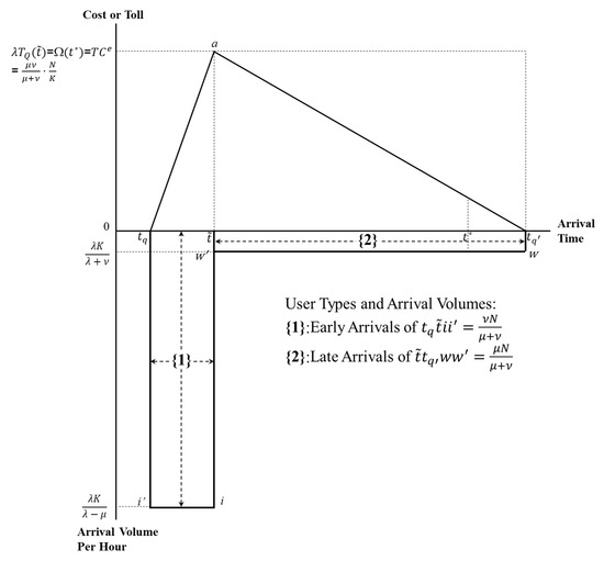
Figure 2.
Queuing time costs and arrival volumes for two types of users before implementation of queuing pricing.
Table 3.
User types, queuing time costs, and arrival volumes before implementation of queuing pricing.
Next, we discuss the number of arrivals, as shown in Table 3. Since the service capacity at the bottleneck field remains at K during the queuing period, the marginal arrival volume of users at the bottleneck entrance can be expressed as . Using Equations (7) and (8) in Section 3, the marginal arrival volumes for early-arriving users and late-arriving users can be obtained as and , respectively. Because the marginal arrival volume refers to the volume of increase or decrease in the number of arrivals per hour, the hourly arrival volume of users can be expressed as . Accordingly, we obtain the hourly arrival volumes for early-arriving and late-arriving users as and , respectively. Subsequently, using Equations (12)–(14) in Section 3, the total number of arrivals for early-arriving users during their early arrival period and for late-arriving users during their late arrival period can be obtained as (=()) and (=()), respectively. Since , the total number of early-arriving users is greater than the total number of late-arriving users, as shown in Table 3, the former is times the latter. This information helps policymakers understand the queuing time cost borne by the two different types of users at the bottleneck entrance before implementing the queuing pricing, as well as the arrival volumes and distribution intervals for different user types.
The above results regarding user types and their respective arrival volumes can be analyzed from below the horizontal axis in Figure 2. User type {1} and {2} respectively represent users who arrive early and late at the bottleneck entrance. Their corresponding arrival intervals are and , respectively. Since the hourly arrival volume of early-arriving users (type {1}) is , and this exceeds the capacity of the bottleneck (), these users must queue at the entrance of the bottleneck. In contrast, the hourly arrival volume of late-arriving users (type {2}) is , which is less than , so the queuing phenomenon in front of the bottleneck gradually eases and eventually dissipates to zero ( = 0).
In Figure 2, the areas of the different regions for {1} and {2} indicate the total number of early-arriving and late-arriving users, respectively. Since (=()) is greater than (=()), the total number of early-arriving users is significantly greater than that of late-arriving users.
The information derived from Figure 2 and Table 3 allows policymakers to estimate the arrival numbers of two types of users—early and late arrivals—within their respective distribution intervals under the pre-toll equilibrium. This supports precise resource allocation, such as manpower and materials, through appropriate deployment strategies.
4.2. Derived Results Under the Optimal Time-Varying Toll Scheme
After implementing the optimal time-varying toll scheme, all user types, their quantities, and related information are shown in Figure 3 and Table 4. Since each user pays a continuous toll () based on their arrival time to ensure zero queuing (, all tolled users can be divided into two main categories: early (including on-time) and late arrivals at the bottleneck entrance, as shown in Equations (16)–(18) in Section 3. In addition, their respective arrival intervals are and . In Figure 3, the vertical heights of the line segments and on the left and right sides of ∆ along the horizontal axis represent the optimal time-varying toll amounts that early and late users must pay. Their slopes are and , respectively (see Equations (16) and (18) in Section 3). Thus, the toll amounts can be obtained as for early users and for late users, as shown in Table 4.
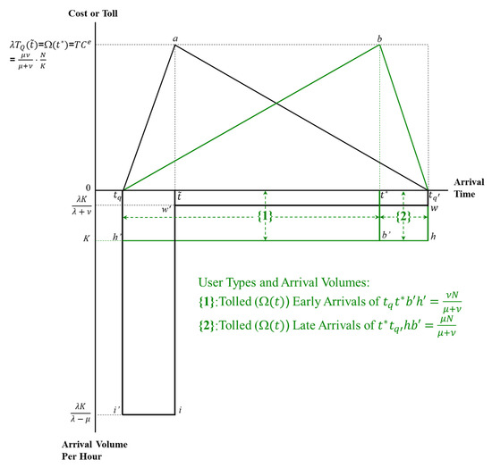
Figure 3.
User types and arrival volumes under optimal time-varying toll scheme.
Table 4.
User types, toll amounts, and arrival volumes under optimal time-varying toll scheme.
Next, we discuss the number of users arriving, as shown in Table 4. After implementing the optimal time-varying toll scheme, there is no longer any queue at the bottleneck entrance (i.e., ), but the service capacity of the bottleneck area remains at . Therefore, the marginal arrival volume of users at the bottleneck entrance is zero (i.e., = ). Based on this, the hourly arrival volume of early or late users (=) is , as shown in Table 4. Subsequently, using Equations (12) and (14), the total arrival volume of early users during their early arrival period and late users during their late arrival period can be obtained as (=()) and (=()), respectively. The former is times the latter, which coincides with the situation in the equilibrium state before the toll implementation.
The aforementioned results regarding user types and their arrival volumes can be analyzed from below the horizontal axis in Figure 3. User types {1} and {2} represent users who arrive early and late at the bottleneck entrance, respectively. Additionally, their arrival areas are distributed over and , respectively. Since the hourly arrival volume for both {1} and {2} users is , which equals the bottleneck capacity, neither group needs to queue at the bottleneck entrance. In Figure 3, the areas representing {1} and {2} users correspond to the total number of early and late arrivals, respectively. As (=()) is greater than (=()), the total number of early users is significantly larger than that of late users.
The information derived from Figure 3 and Table 4 enables policymakers to predict the arrival numbers of different types of tolled users—such as early and late arrivals—within their respective distribution intervals after implementing the optimal time-varying toll scheme. This supports the formulation of relevant supporting measures during the execution of this toll scheme and ensures precise allocation of resources, such as manpower and materials, with an emphasis on timely and appropriate deployment.
4.3. Derived Results Under the Optimal Step Toll Scheme
The optimal step toll scheme is an alternative to the optimal time-varying toll scheme and can be further divided into optimal one-step, two-step, …, n-step toll schemes. Although the optimal n-step toll scheme cannot eliminate the total queueing time for all users at the bottleneck entrance, it can reduce the total queueing time prior to the toll implementation by a factor of . The following Sections will introduce the results of the derivation for user types, their quantities, and related information after the implementation of each version of the optimal step toll scheme.
4.3.1. Optimal One-Step Toll Scheme
After the implementation of the optimal one-step toll scheme, the types and numbers of all users, along with related information, are shown in Figure 4 and Table 5. User types can be divided into five main categories: {1}: free-of-toll and early arrival, {2}: paying the toll and early arrival, {3}: paying the toll and late arrival, {4}: toll evaders (unwilling to pay) and late arrival, and {5}: free-of-toll and late arrival. Their arrival time distributions correspond to the periods , , , and , respectively. Two critical moments appear in the first and fourth time periods: and , which are related to the deliberate behavior of users in the specific periods before the start and the end of the tolling period. The roles of these two critical moments are explained in detail below, along with the corresponding formulas.

Figure 4.
User types and arrival volumes under optimal one-step toll scheme.
Table 5.
User types (five types), queuing time costs, and arrival volumes under optimal one-step toll scheme.
In the queuing pricing model, since the usage flow through the queuing period always remains at the service capacity () of the bottleneck, the first user to pay at must follow immediately behind the last user who does not need to pay before in entering the bottleneck (or reaching their destination). Therefore, their early arrival times are almost the same. Since both must bear the same equilibrium cost (), and the first user to pay at incurs no queuing cost (as is exactly on the left boundary of the optimal time-varying toll triangle, resulting in zero queuing time), the queuing time cost for the last non-paying user before the toll starts must be equal to the toll amount, ρ. This also means the last non-paying user must arrive hours earlier than the first paying user. Assuming the arrival time of the former is , then in the time period hours before (i.e., the interval (, )), no users should arrive at the bottleneck entrance, and thus no queuing time cost line exists during this period. This situation can be seen as a deliberate hedging behavior by non-paying users to avoid the dilemma of facing toll charges while still waiting in line. From this, we can deduce that the no-arrival period (, ) represents the process of the queuing line dissipating to zero at the bottleneck entrance, ensuring that the paying user at can enter the bottleneck without queuing. In summary, after the implementation of the optimal one-step toll scheme, the time value of can be expressed as follows:
In contrast, the cost of the last user who pays at and does not need to queue (since is exactly on the right side of the optimal time-varying toll triangle, the queuing time is zero at this moment) will, in equilibrium, be equal to the cost of the first user who does not need to pay after and follows directly behind him (her). The lateness of both users is almost the same, so the queueing time cost of the first non-paying user after the toll ends will be equal to the toll amount, ρ. However, this situation is impossible unless the first non-paying user had already been waiting for hours before . Let his (her) arrival time be ; it can be understood that a group of users unwilling to pay the toll deliberately start queuing near the bottleneck entrance in sequence from ) and wait until the toll ends before entering. Since the first non-paying user enters the bottleneck immediately after the last paying user when the toll ends () without having to queue, his (her) queuing time cost at the temporary stop near the bottleneck entrance is (). Therefore, after implementing the optimal one-step toll scheme, the time value of can be expressed as follows:
In Table 5, the boundary point () between early and late arrivals appears in the third and fourth time periods. As shown in Figure 4, is exactly located at the intersection of and , representing the bottleneck entrance arrival time that allows users to enter the bottleneck (or arrive at the workplace) on time after implementing the optimal one-step toll scheme. Using the Point–Slope form, the time value of can be expressed as follows:
Next, we will discuss the calculation formulas for the queuing time costs of the aforementioned five types of users. The cost function of the first type of early-arriving user (distributed in the interval ) (as shown in Equation (4)) must be the same as the cost function of the first user ( of the early arrivals under equilibrium conditions. Since = 0, the queuing time cost formula for the first type of user can be derived as . Similarly, the queuing time cost formula for the second type of user () can be derived as .
For the last three types of late-arriving users, the cost function of the third type of user (distributed in the interval ) (as shown in Equation (6)) must be the same as the cost function of the first user () of the late arrivals under equilibrium conditions. Since = , the queuing time cost formula for the third type of user can be derived as . Similarly, the queuing time cost formulas for the fourth type of user () and the fifth type of user () can be derived as and , respectively.
For details on the queuing time cost formulas of the five types of users, as well as the representative line segments and their characteristics, refer to columns 3 to 5 of Table 5. Any point on the blue line segments above the horizontal axis in Figure 4 represents the queuing time costs for these five types of users. Since the slopes of the queuing time cost line segments for all early-arriving users before and after the toll implementation are the same, as shown in Figure 4, overlaps with , and is parallel to . Similarly, since the slopes of the queuing time cost line segments for all late-arriving users before and after the toll implementation are also the same, is parallel to , and (or ) overlaps .
Next, we will discuss the number of users arriving, as shown in Table 5. Since the slope of the queuing time cost line segments for the early-arriving users (either the first or second type) after the toll implementation is the same as that of early-arriving users before the toll implementation, the hourly arrival volume and total arrival volume for each of the two types of users are and , respectively, and the total arrival volume for either the first or second type of users is times the total number of users ().
In contrast, since the slope of the queuing time cost line segments for the late-arriving users (either the third, fourth, or fifth type) after the toll implementation is the same as that of late-arriving users before the toll implementation, the hourly arrival volume for each of the three types of users is . The total arrival volume for the third type of users is , which is times the total number of users (). Subsequently, the total arrival volumes for the fourth and fifth types of users are and , respectively, accounting for and of the total number of users (). As shown in Table 5, the total arrival volume for the fourth-type users is times that for the fifth-type users, with the former being greater than the latter.
The aforementioned results regarding user types and their arrival volumes can be analyzed using the lower part of the horizontal axis in Figure 4. User types {1}−{2} and {3}−{5} respectively represent early- and late-arriving users at the bottleneck entrance. The arrival areas for all user types {1} to {5} are respectively distributed over , , , , and .
According to Figure 4, since overlaps with , the hourly arrival volume (i.e., ) during the interval () is the same as the early arrival period () before the toll implementation. Additionally, since there are no users arriving during the interval (), the hourly arrival volume for that period is zero, and no blue line segment exists.
Furthermore, as shown in Figure 4, since is parallel to and is parallel to , the hourly arrival volumes for tolled users during the intervals () and () are and , respectively, which are the same as the early and late arrival periods before the toll implementation.
Notably, during the arrival period (), in addition to the tolled users, there is also a group of users, with a total of , who queue sequentially near the bottleneck entrance and enter after the end time of the toll (. Since of these toll-evading users overlaps with , their hourly arrival volume is also , making the hourly arrival volume during the period () increase to . Moreover, since overlaps with , the hourly arrival volume of toll-free users during the interval () is the same as the late arrival period () before the toll implementation.
In Figure 4, the area of the different regions corresponding to user types {1} to {5} represents the total number of arrivals for each type. These values can be obtained as follows:, , , , and . By comparing these data, we can determine that the order of the total number of arrivals for each user type is {1} = {2} > {3} > {4} > {5}. Accordingly, it is clear that half of all users will choose to pay to enter the bottleneck after the toll implementation, such as user types {2} and {3}. Among all tolled users, the proportion of those choosing to arrive early (including on time), represented by user type {2}, accounts for , while those choosing to arrive late, represented by user type {3}, account for . Among the remaining half of non-paying users, the proportion of those choosing to arrive early, represented by user type {1}, also accounts for , while the proportion of those choosing to arrive late, represented by user types {4} and {5}, also accounts for .
Meanwhile, as shown in Figure 4, the total arrivals and the distribution of arrival times for each user type after the toll implementation can be easily observed. The arrival periods of early users {1} and {2} are closely adjacent to the time period with no arrivals (, ), with the total number of arrivals on each side being exactly half of the total early arrivals. The arrival periods of late users {3}, {4}, and {5} are positioned next to the right of user {2}, with a two-layer stacked shape as the distinctive feature. Users {3} and {5} are positioned in the lower layer (the first layer), while user {4} is in the upper layer. The total arrivals of user {3} account for 50% of the total late arrivals, while the remaining 50% of late arrivals are made up of users {4} and {5}, with the former having a more arrivals than the latter.
The above information enables policymakers to understand that after the implementation of the optimal one-step toll scheme, in addition to a specific period with no user arrivals, there are five different types of users. Furthermore, the queuing time costs borne by each user type at the bottleneck entrance, as well as the data on the number of arrivals and distribution intervals for each user type, have been clearly determined in the aforementioned analysis. Policymakers can refer to Figure 4 and Table 5 to accurately grasp these data and information, facilitating the formulation of related supporting measures and the precise allocation of various resources (including manpower and materials).
4.3.2. Optimal Two-Step Toll Scheme
After implementing the optimal two-step toll scheme, the types and numbers of all users, along with relevant information, are shown in Figure 5 and Table 6. User types can be categorized into the following eight groups: {1} toll-free and arriving early, {2} paying a low toll () and arriving early, {3} paying a high toll () and arriving early, {4} paying a high toll (2) and arriving late, {5} avoiding high toll (paying low toll) and arriving late, {6} paying a low toll () and arriving late, {7} avoiding low toll (unwilling to pay) and arriving late, and {8} toll-free and arriving late. The arrival time periods for these groups are as follows: , , , , , , , and .Within these periods, four critical times emerge: , , , and . The first two and the latter two are related to users’ intentional behavior in specific periods just before and just after the start and end of the toll scheme. The roles and formulas associated with these four critical times are introduced in detail below.

Figure 5.
User types and arrival volumes under optimal two-step toll scheme.
Table 6.
User types (eight types), queuing time costs, and arrival volumes under optimal two-step toll scheme.
Definitions and derivations of and under the optimal two-step toll scheme can be referenced in the explanation of Equation (22) in Section 4.3.1. Since and are precisely located on the left line of the optimal two-step tolling triangle, users who arrive and pay at and will experience no queuing. Consequently, the non-user intervals (, ) and (, ) represent the dissipation process of the queue in front of the bottleneck entrance, eventually reducing it to zero. Therefore, the time values of and under the optimal two-step toll scheme can be expressed as follows:
Similarly, the definitions and derivations of and can be referenced in the explanation of Equation (23) in Section 4.3.1. Due to users’ intentional avoidance behavior, there will be a group of users avoiding the high toll (willing to pay only the low toll ) and another group avoiding the low toll (unwilling to pay at all). These users begin queuing sequentially at the temporary waiting area near the bottleneck entrance from ) and ), respectively, waiting until the high- and low-toll periods end before entering the bottleneck. Thus, the time values of and under the optimal two-step toll scheme can be expressed as follows:
In Table 6, the fifth and sixth periods indicate the boundary point of early and late arrivals (). As shown in Figure 5, is located precisely at the intersection of and , representing the arrival time that allows users to enter the bottleneck (or arrive at the workplace) on time under the optimal two-step toll scheme. Using the Point–Slope form, the time value of can be expressed as follows:
Subsequently, we analyze the calculation formulas for the queuing time costs associated with the eight categories of users mentioned above. For these categories of early- and late-arriving users, please refer to the derivation of queuing time costs for all users described in Section 4.3.1. Accordingly, the calculation formulas for the queuing time costs of these eight types of users are represented as follows:, , , , , , and . For further details on the cost line segment and line segment characteristics of these eight types of users, please refer to Columns 3 to 5 in Table 6. In Figure 5, each point on each blue line segment above the horizontal axis and its corresponding height represents the queuing time cost for these eight types of users. As shown in Figure 5, the slopes of segments ,, and for early-arriving users are consistent with , while the slopes of , , , , and for the late-arriving users match .
Next, by referring to the detailed explanations of Table 5 in Section 4.3.1, we can infer the arrival volumes of all types of users in Table 6. After implementing the optimal two-step toll scheme, the hourly arrival volume and the total arrival volume for all early-arriving users (the first to third categories) in Table 6 are and , respectively. The total arrival volume for each category of early-arriving users is of the total number of users (N). On the other hand, the hourly arrival volumes for all late-arriving users (the fourth to eighth categories) is , though the total arrival volume varies by category. In Table 6, the total arrival volume for the fourth category of users is , which represents of the total number of users (N). For the fifth or seventh categories and the sixth or eighth categories, the total arrival volumes are and , respectively, accounting for and of the total number of users (N). The former exceeds the latter by a factor of .
The above results regarding the user types and their arrival volumes can be analyzed based on the lower part of the horizontal axis in Figure 5. User types {1}−{3} and {4}−{8} represent users who arrive early and late, respectively, at the bottleneck entrance. Their arrival areas are distributed within their respective blue rectangular blocks. According to Figure 5, since , , and overlap or are parallel with , the hourly arrival volume () for the periods (), () and () is the same as that during the early arrival period () before toll implementation. Additionally, since no users arrive during the periods () and (), the hourly arrival volume for each period is zero, and no blue blocks exist for these two periods.
Similarly, based on Figure 5, as , , , , and are parallel or overlap with , the hourly arrival volume () for the five periods (), (), (), (), and ( is the same as that during the late arrival period (, ) before toll implementation. Notably, during the arrival periods () and (), besides the tolled users, there are two groups, each with a total of users, queuing sequentially at temporary waiting areas near the bottleneck entrance, waiting for the lower toll or toll-free time to enter. Consequently, the hourly arrival volumes for both () and () periods increase to , and for the period (), the hourly arrival volume even rises to .
In Figure 5, the areas of different zones for user types {1} to {8} illustrate the total arrival volumes for each user types. Based on Table 2, these values can be determined as follows: , , , , , , , and . By comparing these values, the order of total arrival volume for each user type is obtained as follows: {1} = {2} = {3} > {4} > {5} = {7} > {6} = {8}. These results reveal that, after implementing the optimal two-step toll scheme, two-thirds of all users will choose to pay for entry into the bottleneck. Among these, the proportion of users opting for the low toll () is one-third. Within this group, those who choose to arrive early (or on time), represented by user type {2}, make up , while those who choose to arrive late, represented by user types {5} and {6}, make up .
Similarly, the proportion of users paying the high toll () is also one-third. Among them, the proportion of those arriving early (or on time), type {3}, is , while those arriving late, type {4}, is . For the remaining one-third of non-paying users, the proportion of early arrivals, type {1}, is , while the proportion of late arrivals, types {7} and {8}, is .
As shown in Figure 5, the arrival blocks and time distribution characteristics of various user types under the optimal two-step toll scheme can be clearly observed. The distribution periods of early-arriving users {1} and {2} are adjacent to the left and right sides of the first non-user arrival period (, ), with each side’s arrival volume accounting for exactly one-third of the total early arrival volume before the toll implementation. Similarly, the distribution periods for early-arriving users {2} and {3} are adjacent to the left and right sides of the next non-user arrival period (, ), where each side’s arrival volume also accounting for one-third of the total early arrival volume before the toll implementation. On the other hand, the distribution periods of late-arriving users {4} to {8} are adjacent to the right side of {3}, displaying a distinct three-layered pyramid shape. Users {4}, {6}, and {8} are positioned on the lower level (first layer), user {5} occupies the middle level (second layer), and user {7} spans both the middle and top layers (third layer). The arrival volume of user {4} constitutes one-third of the total late arrival volume prior to the toll implementation, and the combined arrival volume of either users {5} and {6} or users {7} and {8} also each account for one-third of the total late arrival volume prior to the toll implementation.
The information above enables policymakers to understand that, after implementing the optimal two-step toll scheme, there are not only two specific time intervals without user arrivals but also eight distinct user types. Furthermore, the queuing time costs incurred by each user type before entering the bottleneck, along with data on the arrival volumes and distribution intervals of different user types, have been clearly determined in the above analysis. Policymakers can utilize Figure 5 and Table 6 to accurately grasp these data and insights, facilitating the formulation of relevant support measures and the precise allocation of resources.
4.3.3. Optimal Three-Step Toll Scheme
The derivation process for the optimal three-step toll scheme is similar to that in Section 4.3.1 and Section 4.3.2; therefore, the derivation process is omitted in this Section. Only relevant figure and table are presented for reference by users and policymakers.
As shown in Figure 6 and Table 7, the user types after the implementation of the optimal three-step toll scheme can be categorized into eleven types: {1} toll-free and arriving early, {2} paying a low toll () and arriving early, {3} paying a medium toll () and arriving early, {4} paying a high toll () and arriving early, {5} paying a high toll and arriving late, {6} avoiding high toll (paying medium toll) and arriving late, {7} paying a medium toll and arriving late, {8} avoiding medium toll (paying low toll) and arriving late, {9} paying a low toll and arriving late, {10} avoiding low toll (unwilling to pay) and arriving late, and {11} toll-free and arriving late.
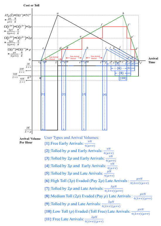
Figure 6.
User types and arrival volumes under optimal three-step toll scheme.
Table 7.
User types (eleven groups), queuing time costs, and arrival volumes under optimal three-step toll scheme.
Moreover, the distribution of the above eleven arrival time periods is as follows: , , , , , , , , , , and . Among these time periods, there are six key moments: , , , , and . The first three and the last three are respectively related to the deliberate behaviors of users in the specific time periods before the start and the end of charging. Referring to the derivation process related to user avoidance behaviors in the optimal one- and two-step toll schemes, the time values of the six moments under the optimal three-step toll scheme can be obtained.
4.3.4. Optimal n-Step Toll Scheme
To understand the types, quantities, and related information for all users under the optimal n-step toll scheme, one only needs to compare the derived results from the optimal one-, two-, and three-step toll schemes. By comparing Table 5, Table 6 and Table 7, user classifications under the optimal n-step toll scheme can be categorized as follows: {1} toll-free and arriving early, {2} paying and arriving early, {3} paying and arriving early, {4} paying and arriving early, …, {n + 1} paying and arriving early, {n + 2} paying and arriving late, {n + 3} avoiding (paying ) and arriving late, {n + 4} paying and arriving late, {n + 5} avoiding (paying ) and arriving late, {n + 6} paying and arriving late, {n + 7} avoiding (paying ) and arriving late, {n + 8} paying and arriving late, {n + 9} avoiding (paying and arriving late, …, {2n + 1} paying and arriving late, …, {3n + 1} avoiding (unwilling to pay) and arriving late, and {3n + 2} toll-free and arriving late. In total, there are (3n + 2) user groups, as shown in Table 8, including n groups of toll-paying early arrivals, n groups of toll-paying late arrivals (in light blue), and n groups of opportunistic late arrivals, along with two groups exempt from toll and arriving either early or late. For the arrival periods of each user type, please refer to the first column of Table 8.
Table 8.
User types ((3n + 2) groups), queuing time costs, and arrivals under optimal n-step toll scheme.
Among the arrival periods for the aforementioned (3n + 2) groups of users, there are 2n critical moments: , , , …, and , , , …, . The former and the latter are associated with the deliberate behavior of users in the n specific periods before the toll begins and ends, respectively. Based on the derived results from the optimal one-, two-, and three-step toll schemes regarding the deliberate avoidance behavior of early-arriving users, this can be extended to the optimal n-step toll scheme. Thus, there will be n periods with no user arrivals: (, ), (, ), …, (, ), and each period’s length is equal to the lowest toll () divided by the hourly queuing time cost (λ). Specifically, under the optimal n-step toll scheme, there exists a period with no user arrivals () before the start time of each different toll. The duration of this period is , ensuring that users arriving at the exact start time of each different toll (precisely on the left side of optimal time-varying toll line) can enter the bottleneck without queuing. Consequently, each no-arrival period will result in the complete dissipation of the queuing line in front of the bottleneck entrance. Based on the above analysis and the values provided in Table 2, the start time of each no-arrival period can be expressed as follows:
Similarly, based on the previously derived results for the deliberate avoidance behavior of late-arriving users under the optimal one-, two-, and three-step toll schemes, this approach can be extended to the optimal n-step toll scheme. Consequently, there will be n opportunistic arrival intervals: (, ), (, ), …, (, ). During these intervals, users will deliberately avoid entering the bottleneck to evade higher tolls and instead wait until the next step with a lower toll (or toll-free) before entering. The duration of each of these intervals is also determined by the minimum toll () divided by the hourly queuing time cost (λ). Specifically, prior to the end time of each different toll, there is an opportunistic arrival interval (= with a duration of , ensuring that users arriving exactly at the end time of each different toll (precisely on the right side of optimal time-varying toll line) can enter the bottleneck without queuing. This indicates that each opportunistic arrival interval can fully clear any queue of users willing to pay a higher toll at the bottleneck entrance. Based on the above analysis and the values in Table 2, the starting time of each late arrival interval for each group of users who intentionally avoid entering the bottleneck can be expressed as follows:
In Table 8, the boundary point () between the (n + 1) and (n + 2) time intervals represents the arrival time at the bottleneck entrance that allows users to enter the bottleneck on time (or arrive at the workplace punctually) under the optimal n-step toll scheme. Using the Point–Slope form, the time value of can be expressed as follows:
According to Table 8, under the optimal n-step toll scheme, the hourly arrival volume and total arrival volume for all early-arriving users (types 1 through n) are and , respectively. The total arrival volume for each type of early-arriving user is of the total number of users (N). On the other hand, for all late-arriving users (types {n + 2} through {3n + 2}), the hourly arrival volume is , though the total arrival volume differs for each user type. The total arrival volume for type {n + 2} users is , which is of the total number of users (N). The total arrival volumes for type {n + 3}, {n + 5}, {n + 7}, … or {3n + 1} users as well as type {n + 4}, {n + 6}, {n + 8}, …or {3n + 2} users are and , respectively, accounting for and of the total number of users (N). The former group is (greater than 1) times the latter group. Additionally, the combined total arrival volume for type {n + 3} and {n + 4} users, type {n + 5} and {n + 6} users, …, or type {3n + 1} and {3n + 2} users is equal to the total arrival volume for type {n + 2} users, which is of the total user population. Finally, based on Table 8, the total arrival volume ranking among user types is as follows: {1} = {2} = {3} = …. = {n + 1} > {n + 2} > {n + 3} = {n + 5} = {n + 7} = …. = {3n + 1} > {n + 4} = {n + 6} = {n + 8} = …. = {3n + 2}.
According to Table 8, a proportion of of all users would choose to pay to access the bottleneck under the optimal n-step toll scheme. The proportion of users opting to pay the toll at each step is . Among these paying users, the proportion choosing to arrive early (including on time) is , while those choosing to arrive late account for . For the remaining of non-paying users, the proportion who arrive early is also , and those who arrive late account for .
Although it is challenging to show a figure related to the queuing time costs and total arrival volumes for each user type after implementing the optimal n-step toll scheme, the structure of the arrival volumes and time distribution for each user type can be anticipated based on the regular patterns observed from Figure 3, Figure 4 and Figure 5. The distribution intervals of the two consecutive groups of early-arriving users are located on either side of a period with no user arrivals, continuing up to the types {n} and {n + 1} users, where early-arriving users are distributed on both sides of the interval (, ) with no arrivals. The total volume on each side exactly represents of the total number of users (N).
On the other hand, the distribution periods for late-arriving users, from type {n + 2} to {3n + 2} users, are positioned adjacent to the right of type {n + 1} users, forming a distinct (n + 1)-layer pyramid structure. The bottom layer of this (n + 1)-layer pyramid includes types {n + 2}, {n + 4}, {n + 6}, …, and {3n + 2} users. The second layer has one fewer type of users than the bottom layer, consisting of types {n + 3}, {n + 5}, {n + 7}, …, and {3n + 1} users. The third layer contains one type fewer than the second, including the remaining types from the second layer: types {n + 5}, {n + 7}, {n + 9}, …, and {3n + 1} users. The fourth layer similarly reduces by one type of users compared to the third layer, encompassing the remaining types from the third layer: types {n + 7}, {n + 9}, {n + 11}, …, and {3n + 1} users. This sequential reduction continues upward, stacking until only the type {3n + 1} users remain at the top of the pyramid structure.
The information derived from Table 8 enables policymakers to understand that, following the implementation of the optimal n-step toll scheme, in addition to n specific time intervals with no user arrivals, there are also (3n + 2) distinct types of users. According to Table 8, policymakers can accurately determine the queuing time costs incurred by each user type before entering the bottleneck, along with data on arrival volumes and distribution intervals. This information facilitates the development of supporting measures and the precise allocation of resources.
4.4. Numerical Analysis
This Section presents a numerical example of road queuing pricing to demonstrate the results obtained in the preceding Sections. Although this numerical analysis is not based on micro-level individual data, the scenario reflects realistic traffic conditions in urban Taiwan. The total number of 3600 vehicles corresponds to typical peak-hour volumes at major urban bottlenecks, such as those observed at Taipei’s Zhongxiao Bridge or Taichung’s Wuquan Interchange. The assumed bottleneck capacity of 1800 vehicles per hour aligns with standards from the MOTC for a single-lane arterial under peak congestion. Furthermore, the hourly cost parameters are adapted from Small [2] and adjusted to 2024 values using the U.S. inflation index, ensuring reasonable behavioral sensitivity assumptions.
Assume there are 3600 homogeneous commuters (N), each driving a vehicle, and all of them need to pass through a bottleneck segment operating at full capacity before reaching their destinations. The capacity of the bottleneck is K = 1800 vehicles per hour. From Equation (11), it can be inferred that the total queueing time for all commuters at the bottleneck entrance (i.e., the duration from the start to the end of the queue) will last for two hours (N/K = 2 hrs). Additionally, assume all commuters start work at 8:30 a.m. (=) and that their hourly costs of queueing, early arrival, and late arrival are respectively assumed to be = USD 19.2, = USD 11.7 and = USD 45.63. These three values are based on a survey conducted by Small [2] of 572 commuters in the San Francisco Bay Area, where the original hourly costs were USD 6.4, USD 3.9, and USD 15.21, respectively. Adjusting for inflation, where the purchasing power of USD 1 in 1982 is approximately equivalent to USD 3 in 2024, these original values are multiplied by 3 to obtain the assumed values of , and .
Based on the above values, we can use Equations (12) and (14) to calculate the start and end times of queueing for all commuters are 6:54:36 a.m. (=6.91 h = ) and 8:54:36 a.m. (=8.91 h = ), respectively. Furthermore, using Equation (15), the equilibrium cost for each commuter can be calculated as USD 18.63 (=). Since commuters arriving at the bottleneck entrance at and incur no queueing time costs when entering the bottleneck, they bear the highest costs of early arrival and late arrival, respectively, both amounting to USD 18.63. Additionally, according to Equation (13), commuters arriving at the bottleneck entrance at 7:31:48 a.m. (=7.53 h = ) can enter the bottleneck (or reach their workplace) exactly on time at 8:30 a.m. (=8.50 h = ) but must bear the highest queueing time cost of USD 18.63. Commuters arriving at times other than , , and at the bottleneck entrance bear a combined cost of USD 18.63, which includes both queueing time costs and early (or late) arrival costs. The above time values of , , and represent the arrival times at the bottleneck entrance in hours, measured from midnight (0:00).
In the equilibrium state prior to the implementation of queuing pricing, as detailed in the aforementioned Table 3, the information regarding the types of all users (two types), queueing time costs and the number of arrivals is shown from the first to second columns of Table 9. Please also refer to the illustration in Figure 2.
Table 9.
User types, queuing time costs, and arrivals before and after implementing queuing pricings.
After the implementation of the optimal time-varying toll scheme, as detailed in the aforementioned Table 4, the information regarding the types of all users (still two types), queueing time costs and the number of arrivals is shown from the third to fourth columns of Table 9. Please also refer to the illustration in Figure 3.
Additionally, after the implementation of the optimal two-step toll scheme, as detailed in the aforementioned Table 6, the information regarding the types of all users (eight types), queueing time costs and the number of arrivals is shown from the fifth to fourteenth columns of Table 9. Please also refer to the illustration in Figure 5.
In Table 9, all user types, arrival time distributions, total arrivals in each time period, and their characteristics can be compared before and after the implementation of queuing pricings, highlighting the differences among these factors. Before the toll implementation and under the optimal time-varying toll scheme, user types, user numbers, and their characteristics remain straightforward. However, after implementing the optimal two-step toll scheme, the situation becomes more complex: user types increase from two before tolling to eight, and user numbers increase from two categories before tolling to four. The changes in scenarios caused by the implementation of queuing pricing (especially optimal step toll schemes) will inevitably compel the bottleneck management authorities to adjust their existing allocation of human and material resources.
Using Table 9 as an example, after implementing the optimal two-step toll scheme, there will be two time intervals, each lasting 19.2 min, during which no users arrive at the bottleneck entrance. Similarly, there will be two time intervals, each lasting 19.2 min, during which users deliberately avoid entering the bottleneck. These phenomena do not occur under the non-toll equilibrium nor under the optimal time-varying toll scheme.
As shown in Table 9, users paying high tolls for early and late arrivals are distributed across two periods: (7:58−8:11) and (8:11−8:38), with user numbers of 955 and 245, respectively. Users paying the low tolls are distributed across three periods: (7:26−7:39), (8:11−8:38), and (8:38−8:46). The first period represents early arrivals with 955 users, while the second and third periods represent late arrivals with 172 and 73 users, respectively.
Users exempt from tolls are distributed across three periods: (6:55−7:07), (8:27−8:46), and (8:46-8:55). The first period represents early arrivals with 955 users, while the second and third periods represent delayed arrivals with 172 and 73 users, respectively.
In summary, the arrival numbers for the three types of users—those paying high tolls (Types {3} and {4}), those paying low tolls (Types {2}, {5}, and {6}), and those exempt from tolls (Types {1}, {7}, and {8})—are all equal, each accounting for one-third of the total arrivals (3600 users) in the pre-tolling equilibrium state.
Figure 7 presents a comparative visualization of user arrival volumes per hour under three queuing pricing scenarios: (1) non-toll equilibrium, (2) optimal time-varying toll scheme, and (3) optimal two-step toll scheme. In all cases, arrival times are aligned relative to the preferred arrival time, with each interval labeled to indicate whether it corresponds to early or late arrival behavior. The non-toll and time-varying toll scenarios exhibit relatively simple and symmetric arrival patterns, with users either arriving early or late around the preferred time. In contrast, the two-step toll scheme induces a more complex arrival distribution, introducing eight distinct user types—including tolled and toll-free early and late arrivals, as well as toll evaders. Each bar represents the number of users arriving during a specific time interval, highlighting how different tolling strategies influence arrival distribution. Notably, the step toll scheme results in more dispersed and complex arrival patterns, which has important implications for operational planning and resource allocation at bottleneck locations.
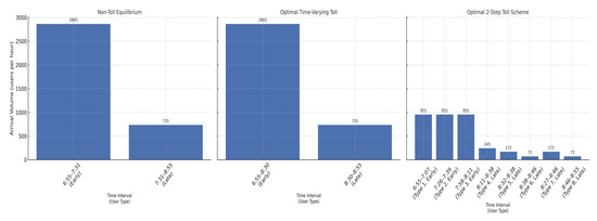
Figure 7.
Hourly arrival volumes under non-toll equilibrium, optimal time-varying toll, and optimal two-step toll schemes.
The aforementioned changes in scenarios before and after implementing the optimal two-step toll scheme can serve as strategic references for bottleneck management authorities. These insights are particularly valuable for formulating strategies related to resource allocation and flexible scheduling. Policy implementation units can precisely deploy the appropriate amount of manpower and resources during different time periods to match the number of users in each period, thereby enhancing efficiency management and risk control once the queuing pricing policy is implemented.
The reliability and practical applicability of the numerical results in Table 9 are supported by two aspects. First, all values are calculated based on three key parameters—the hourly costs of queuing, early arrival, and late arrival—which respectively represent opportunity and penalty costs. The calibration of these parameters ensures the objectivity and accuracy of the numerical results. Second, all results are derived under the principle of equilibrium cost conservation, whereby users adjust their arrival times to maintain a consistent cost before and after toll implementation. This principle is well-established in economics and serves as a robust theoretical foundation for behavioral prediction.
While the current study focuses on theoretical derivations and scenario-based simulation, the model’s behavioral implications align well with established findings in the bottleneck pricing literature. In future work, empirical validation may be conducted using observed vehicle arrival data at toll plazas or port entries where dynamic pricing is in place. Comparative studies could also be explored by calibrating the model for different urban locations (e.g., Taipei vs. Kaohsiung) or applying alternative tolling designs (e.g., coarse toll or reservation-based pricing) to assess efficiency and distributional effects across policy options.
5. Conclusions
Queuing pricing is a tolling strategy developed to address user congestion at bottleneck facilities such as commuter corridors and canal channels. Over the past five decades, its theoretical foundations and practical applications have been extensively studied. Two principal schemes—the optimal time-varying toll and the optimal step toll—have emerged, each with specific strengths and limitations depending on the desired level of queuing mitigation. However, while the existing literature has focused heavily on toll design and efficiency outcomes, critical post-implementation issues—such as user classification, temporal distribution, compliance and avoidance behavior—remain underexplored. These factors are vital for informing policy support mechanisms and ensuring the efficient allocation of resources during policy rollout.
This study first classifies users under the two tolling schemes. Under the optimal time-varying toll scheme, where all users are tolled continuously based on their arrival times, users can be divided into two groups: early (including on-time) and late arrivals. In contrast, the optimal step toll scheme, which allows toll-free periods and varying step-based tolls, results in four user subgroups: toll-payers and non-payers, each further divided into early (including on-time) and late arrivals.
The behavioral dynamics under each scheme are then examined. Under the optimal time-varying toll, users’ decisions reflect individual optimization—where zero queuing time is internalized into toll payments. Since queuing is eliminated, each user’s arrival at the bottleneck matches their intended destination arrival time. Importantly, the number of early and late arrivals under this toll scheme mirrors that in the non-toll equilibrium.
User behavior under the step toll scheme is more complex, comprising compliant behavior and deliberate avoidance. Compliant users shift their arrivals forward or backward in time in response to tolls. This study derives the scheduled (on-time) arrival points for each n-step toll scheme (where n = 1, 2, 3, …), providing reference boundaries for classifying early and late arrivals. In contrast, avoidance behavior manifests in two specific patterns: (1) time intervals before each toll step begins, during which no early arrivals occur as users attempt to avoid higher upcoming tolls, and (2) time intervals near the end of each toll step, during which opportunistic latecomers delay entry to take advantage of the next lower toll (or toll-free) period. This paper derives the start times and uniform durations of these avoidance intervals, each equal to the first-step toll divided by the queuing time cost per hour.
Quantitatively, this study confirms that the distribution of early and late arrivals under the optimal time-varying toll remains consistent with the no-toll equilibrium. However, under the optimal n-step toll scheme, user groups expand to 3n + 2 categories: n groups of tolled early arrivals, n tolled late arrivals, n opportunistic late arrivals, and two toll-free groups (early and late). The arrival intervals and user volumes for each group are calculated. Notably, the total number of tolled users per step is uniformly distributed as 1/(n + 1) of the total number of users, and the toll-free users (both early and late) also constitute 1/(n + 1) of the total number of users.
This comprehensive framework for user classification, behavioral analysis, and volume estimation—covering both compliance and avoidance patterns—fills a significant gap in the queuing pricing literature. The regularities and structures uncovered here enhance the theoretical robustness of queuing models and provide practical guidance for policy implementation. Policymakers can use these findings to allocate human and material resources more precisely across time periods, ensuring effective policy execution, minimizing waste, and achieving the intended reductions in queuing time.
From a policy and managerial perspective, the findings of this study enable bottleneck facility managers to anticipate arrival patterns and implement proactive staffing or scheduling strategies. The identification of toll-free periods, toll avoidance intervals, and uniform group sizes across toll steps allows for precise resource allocation during peak and off-peak periods. Moreover, the step-based toll structure strikes a balance between effectiveness and feasibility, making it suitable for implementation in areas without advanced dynamic tolling systems. Understanding how different toll levels influence early and late arrival behavior also helps design complementary support strategies during policy rollout.
A clear limitation of this study is that the proposed queuing pricing model is restricted to a single bottleneck with no alternative routes, which may limit its applicability in more complex networks. This situation is especially relevant for urban commuting corridors, where detours are often impractical due to higher time and fuel costs. Furthermore, this study assumes homogeneous users and linear time-related costs. The derived results regarding user classification and behavior may shift considerably when user heterogeneity or stochastic events are introduced.
Future research could extend the model by incorporating heterogeneous users with diverse value-of-time, schedule preferences, or travel behaviors, which would enhance behavioral realism and broaden applicability. Integrating demand uncertainty and network effects would further improve robustness. Moreover, empirical validation using observed vehicle or ship arrival data could substantiate the model’s predictive power. Comparative studies across cities or transport modes—such as Taipei vs. Kaohsiung, or road vs. port access—would help evaluate the generalizability and distributional impacts of queuing pricing schemes.
Funding
This research received no external funding.
Data Availability Statement
Data available in a publicly accessible repository.
Conflicts of Interest
The author declares no conflict of interest.
References
- Vickrey, W.S. Congestion theory and transport investment. Am. Econ. Rev. 1969, 59, 251–260. [Google Scholar]
- Small, K.A. The scheduling of consumer activities: Work trips. Am. Econ. Rev. 1982, 72, 467–479. [Google Scholar]
- Arnott, R.; De Palma, A.; Lindsey, R. Economics of a bottleneck. J. Urban Econ. 1990, 27, 111–130. [Google Scholar] [CrossRef]
- Laih, C.H. Queueing at a bottleneck with single-and multi-step tolls. Transp. Res. Part A 1994, 28, 197–208. [Google Scholar] [CrossRef]
- Bao, Y.; Xiao, F.; Gao, Z.; Gao, Z. Investigation of the traffic congestion during public holiday and the impact of the toll-exemption policy. Transp. Res. Part B 2017, 104, 58–81. [Google Scholar] [CrossRef]
- Li, C.; Lu, Y.; Wang, Y.; Jiang, G. Congestion behavior and tolling strategies in a bottleneck model with exponential scheduling preference. Elec. Res. Arch. 2022, 31, 1065–1088. [Google Scholar] [CrossRef]
- Liu, Q.; Van Den Berg, V.A.C.; Verhoef, E.T.; Jiang, R. Pricing in the stochastic bottleneck model with price-sensitive demand. Transp. Res. Part B 2025, 194, 103176. [Google Scholar] [CrossRef]
- Deng, Y.; Li, Z.C.; Qian, S.; Ma, W. Modeling the curbside congestion effects of ride-hailing services for morning commute using bi-modal two-tandem bottlenecks. arXiv 2025, arXiv:2506.09466. [Google Scholar] [CrossRef]
- Lindsey, C.R.; Van Den Berg, V.A.C.; Verhoef, E.T. Step tolling with bottleneck queuing congestion. J. Urban Econ. 2012, 72, 46–59. [Google Scholar] [CrossRef]
- Van Den Berg, V.A.C. Coarse tolling with heterogeneous preferences. Transp. Res. Part B 2014, 64, 1–23. [Google Scholar] [CrossRef]
- Small, K.A. The bottleneck model: An assessment and interpretation. Econ. Transp. 2015, 4, 110–117. [Google Scholar] [CrossRef]
- Li, Z.-C.; Lam, W.H.K.; Wong, S.C. Step tolling in an activity-based bottleneck model. Transp. Res. Part B 2017, 101, 306–334. [Google Scholar] [CrossRef]
- Li, Z.C.; Yu, D.P.; De Palma, A. Bottleneck congestion and urban spatial structure with heterogeneous households: Equilibrium, capacity expansion and congestion tolling. J. Urban Econ. 2024, 144, 103693. [Google Scholar] [CrossRef]
- Yu, X.; Van Den Berg, V.A.C.; Verhoef, E.T. Preference heterogeneity in a dynamic flow congestion model. Transp. Res. Part B 2025, 195, 103193. [Google Scholar] [CrossRef]
- Laih, C.H.; Sun, P.Y. The optimal toll scheme for ships queuing at the entrance of Panama Canal. Marit. Econ. Logist. 2014, 16, 20–32. [Google Scholar] [CrossRef]
- Venturini, G.; Iris, C.; Kontovas, C.A.; Larsen, A. The multi-port berth allocation problem with speed optimization and emission considerations. Transp. Res. Part D 2017, 54, 142–159. [Google Scholar] [CrossRef]
- Du, Y.; Meng, Q.; Shi, W. Impact analysis of the traffic convoy system and toll pricing policy of the Suez Canal on the operations of a liner containership over a long-haul voyage. Int. J. Shpg. Trans. Logist. 2019, 11, 119–144. [Google Scholar] [CrossRef]
- Deng, Y.; Sheng, D.; Liu, B. Managing ship lock congestion in an inland waterway: A bottleneck model with a service time window. Transp. Policy 2021, 112, 142–161. [Google Scholar] [CrossRef]
- Wang, T.; Li, T. Ship lock management and dynamic congestion toll for ships. Ocean Coast. Manag. 2022, 230, 106369. [Google Scholar] [CrossRef]
- Duldner-Borca, B.; van Hassel, E.; Putz-Egger, L.M. Understanding the effects of resolving nautical bottlenecks on the Danube: A KPI-based conceptual framework. Eur. Transp. Res. Rev. 2023, 15, 23. [Google Scholar] [CrossRef]
- Li, Z.C.; Huang, H.J.; Yang, H. Fifty years of the bottleneck model: A bibliometric review and future research directions. Transp. Res. Part B 2020, 139, 311–342. [Google Scholar] [CrossRef]
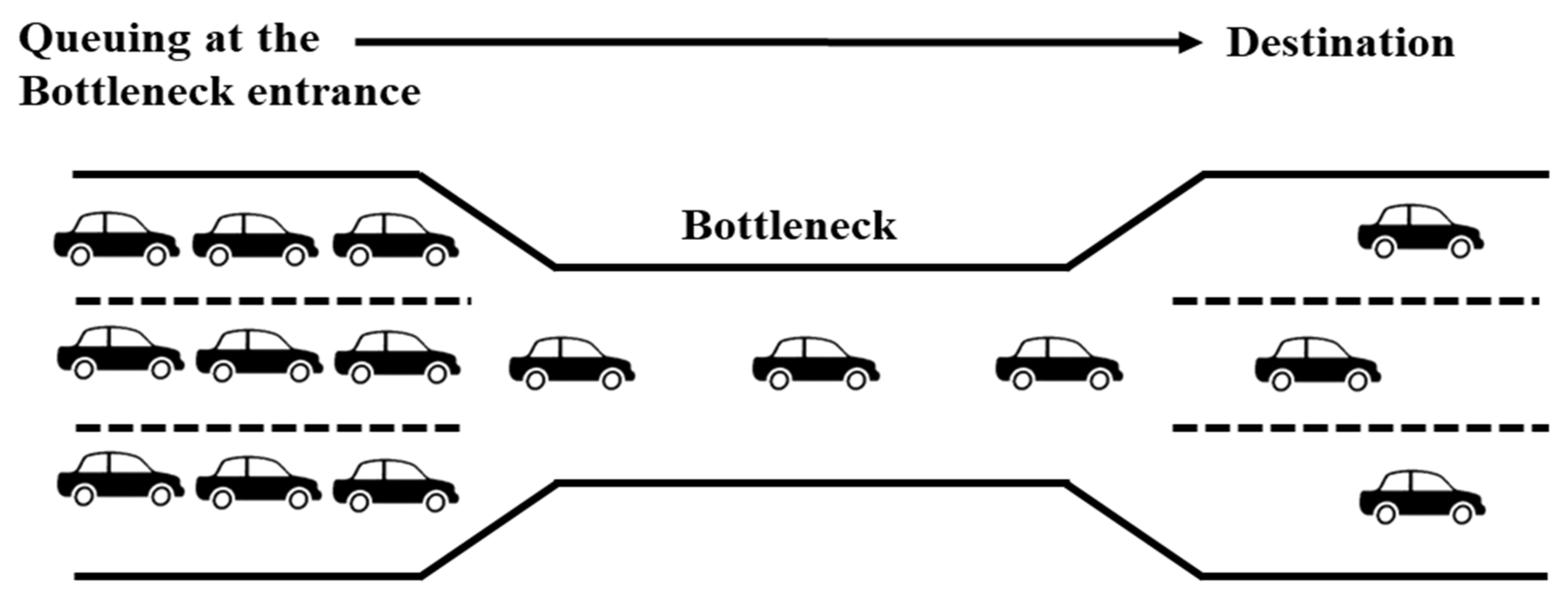


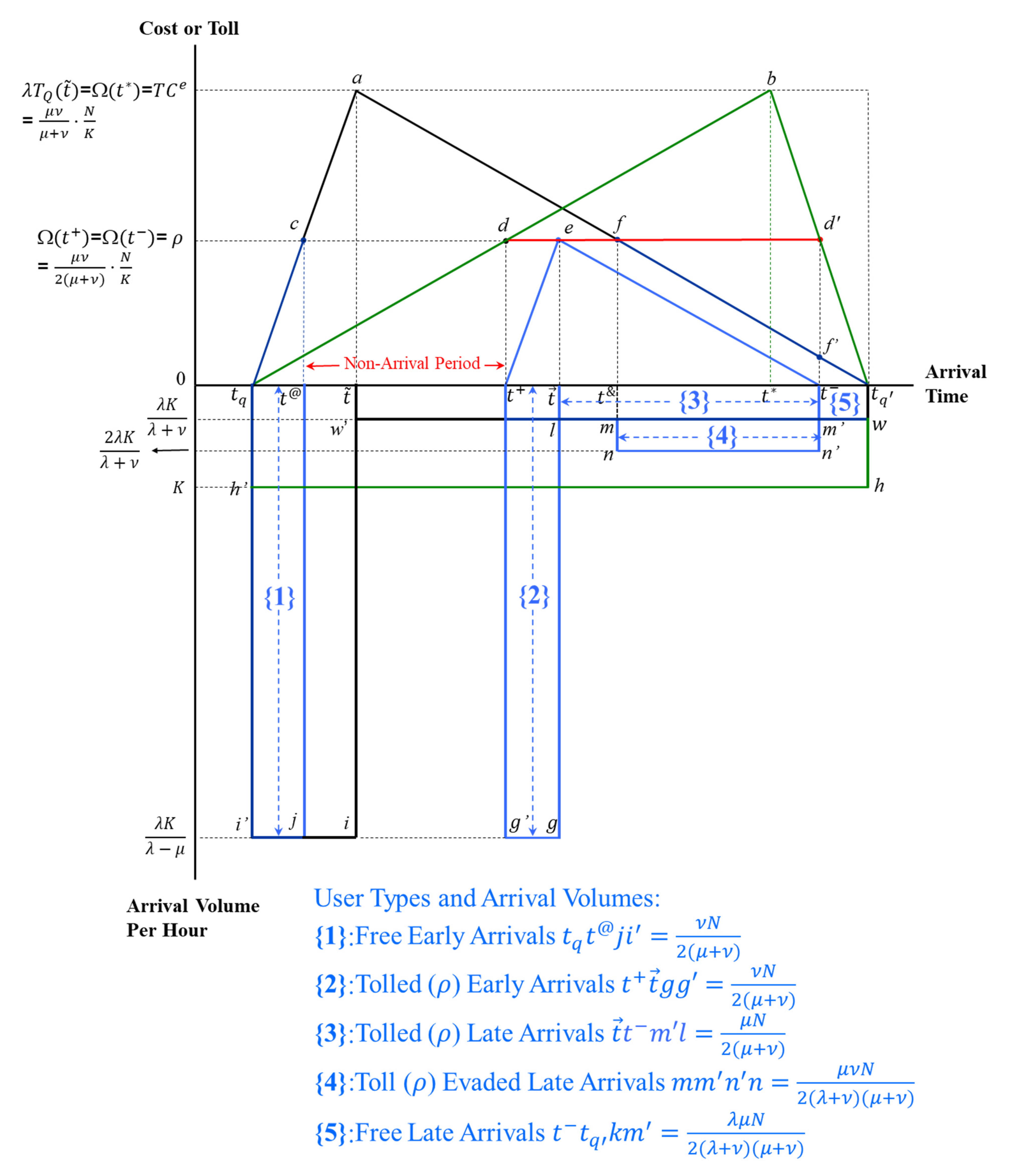
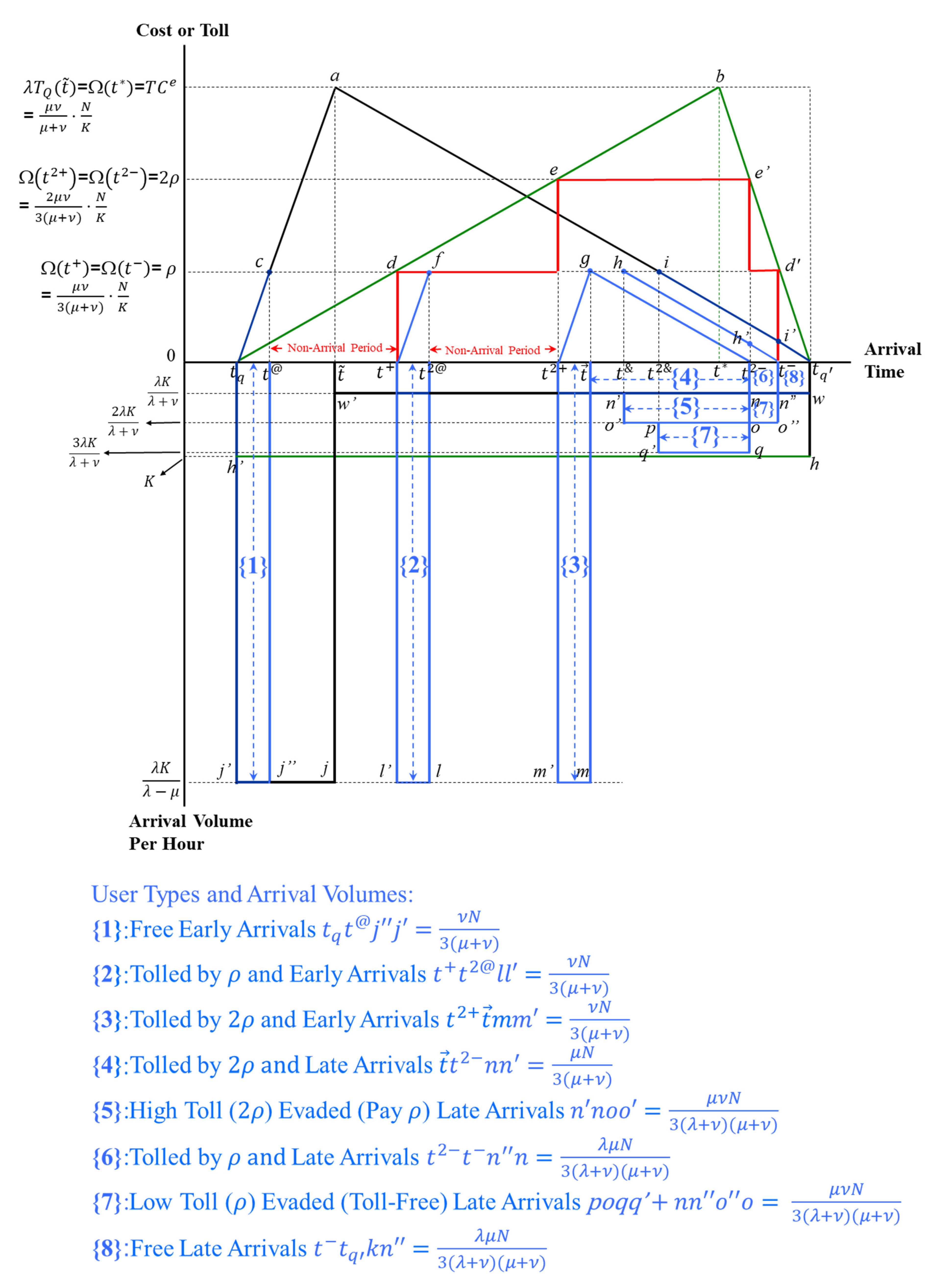
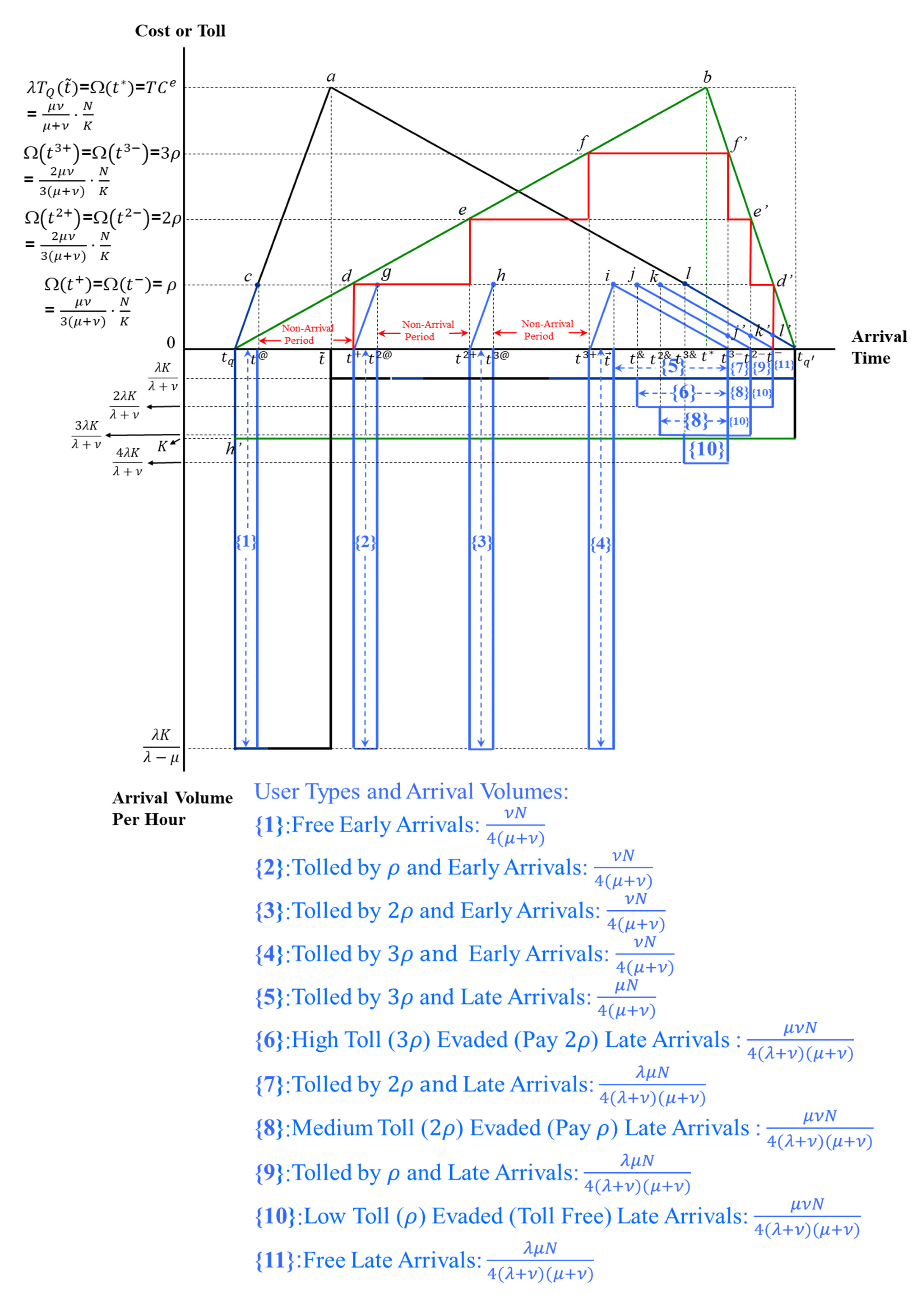
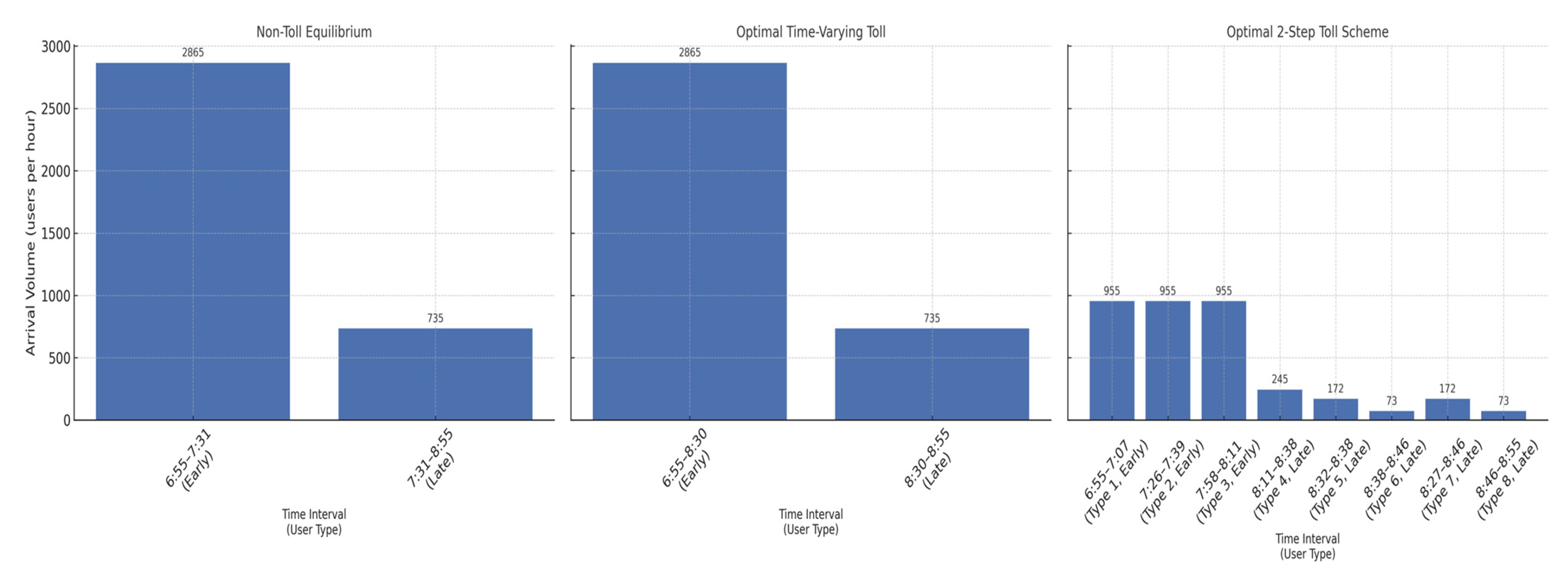
Disclaimer/Publisher’s Note: The statements, opinions and data contained in all publications are solely those of the individual author(s) and contributor(s) and not of MDPI and/or the editor(s). MDPI and/or the editor(s) disclaim responsibility for any injury to people or property resulting from any ideas, methods, instructions or products referred to in the content. |
© 2025 by the author. Licensee MDPI, Basel, Switzerland. This article is an open access article distributed under the terms and conditions of the Creative Commons Attribution (CC BY) license (https://creativecommons.org/licenses/by/4.0/).