A Robust System for Super-Resolution Imaging in Remote Sensing via Attention-Based Residual Learning

Abstract

Deep learning-based super-resolution (SR) frameworks are widely used in remote sensing applications. However, existing SR models still face limitations, particularly in recovering contours, fine features, and textures, as well as in effectively integrating channel information. To address these challenges, this study introduces a novel residual model named OARN (Optimized Attention Residual Network) specifically designed to enhance the visual quality of low-resolution images. The network operates on the Y channel of the YCbCr color space and integrates LKA (Large Kernel Attention) and OCM (Optimized Convolutional Module) blocks. These components can restore large-scale spatial relationships and refine textures and contours, improving feature reconstruction without significantly increasing computational complexity. The performance of OARN was evaluated using satellite images from WorldView-2, GaoFen-2, and Microsoft Virtual Earth. Evaluation was conducted using objective quality metrics, such as Peak Signal-to-Noise Ratio (PSNR), Structural Similarity Index Measure (SSIM), Edge Preservation Index (EPI), and Perceptual Image Patch Similarity (LPIPS), demonstrating superior results compared to state-of-the-art methods in both objective measurements and subjective visual perception. Moreover, OARN achieves this performance while maintaining computational efficiency, offering a balanced trade-off between processing time and reconstruction quality.

1. Introduction

High-resolution remote sensing imagery has become an important source of geoinformation, playing a vital role in various applications, including environmental monitoring, urban planning, crop identification, building extraction, and the detection of small objects, among others [1,2,3,4].

These images enable a detailed analysis of spatial and temporal patterns, which are essential for informed decision-making in precision agriculture, natural resource management, and disaster monitoring [3]. For example, precise vegetation detection enables crop health assessment and irrigation planning. At the same time, urban analysis facilitates the identification of key infrastructure and monitoring changes in population density [5,6]. However, the acquisition of high-resolution (HR) images faces significant challenges due to the limitations of remote sensing hardware. These systems are susceptible to platform vibrations, optical diffraction, and noise interference, resulting in blurred images with a loss of information [4].

To mitigate these limitations, an alternative solution is to apply super-resolution (SR) techniques to enhance the spatial quality of the imagery. This approach is more viable than upgrading satellite and optical sensors, which is often infeasible due to the high cost and complexity of implementing new acquisition systems. Consequently, super-resolution provides a cost-effective alternative for achieving the desired image quality without requiring modifications to the sensing hardware.

Super-resolution techniques have gained popularity as an effective alternative for reconstructing HR images from low-resolution (LR) ones, which enhances image quality without requiring new sensors. A point worth mentioning is that the input LR images are assumed to be free from substantial noise that could interfere with the SR process.

Super-resolution techniques are classified into three main approaches: interpolation-based, reconstruction-based, and deep learning-based methods [7]. Among the deep learning-based methods, Convolutional Neural Networks (CNNs) have proven to be powerful tools for super-resolution, outperforming traditional methods due to their ability to learn complex patterns in the mapping between HR and LR images in a supervised manner, achieving better results in terms of visual fidelity and recovering high-frequency information more effectively [8].

Some classic models, such as SRCNN [9], VDSR [10], and EDSR [11], have established themselves as foundational in super-resolution, demonstrating the capability of these methods to reconstruct fine details. Subsequently, SRResNet, proposed by Leding et al. [12], introduced deep residual architectures, showcasing their ability to recover fine details with greater visual fidelity. Although these networks are effective on natural images, applying these methods to remote sensing images still presents challenges, such as the presence of noise, integrating information across channels, and reconstructing contours and textures.

In addition to CNN-based methods, the literature also includes Generative Adversarial Network (GAN)-based models, which aim to improve perceptual quality through adversarial training. For example, PCA-SRGAN [13] introduces a principal component projection mechanism into the discriminator, enabling the generator to progressively reconstruct image features from coarse structure to fine texture by leveraging orthogonal projections of facial data, thus enhancing contour clarity and texture realism. Similarly, NVS-GAN [14] incorporates architectural components such as identity skip connections, bilinear sampling, and depthwise separable convolutions and is optimized using a combination of loss functions (MAE, SSIM, and Huber loss), resulting in efficient models with reduced computational cost.

However, despite their potential, GAN-based models often struggle to produce geometrically accurate textures and may generate visually plausible but spatially incorrect features [13]. This limitation is particularly problematic in remote sensing tasks, where preserving authentic spatial information is essential for downstream applications, such as land cover classification, change detection, or urban analysis.

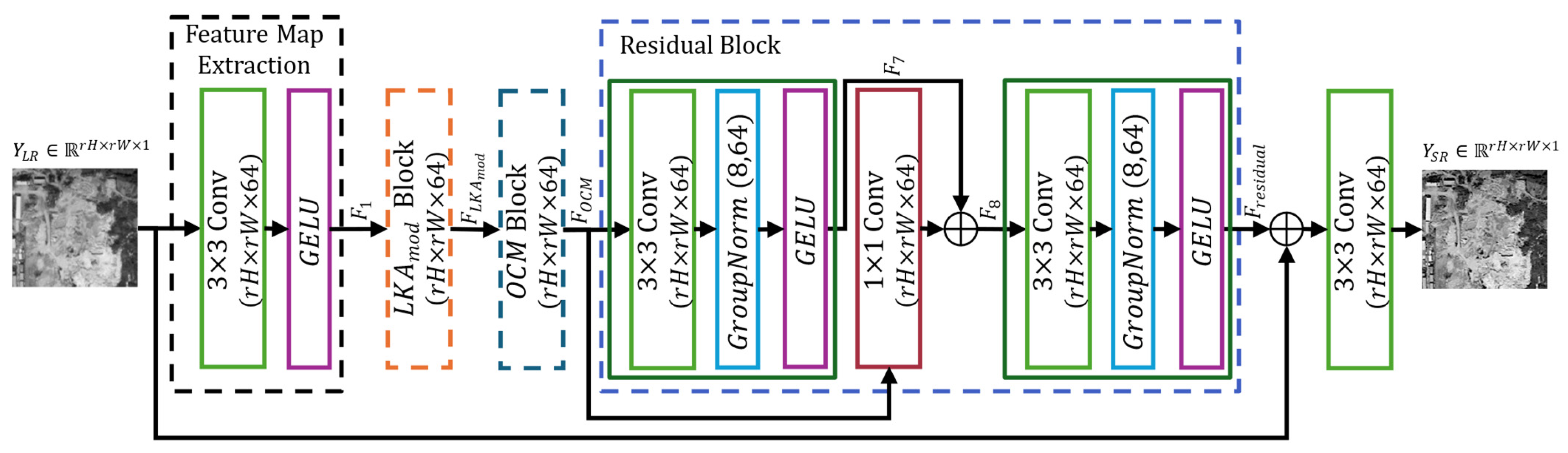
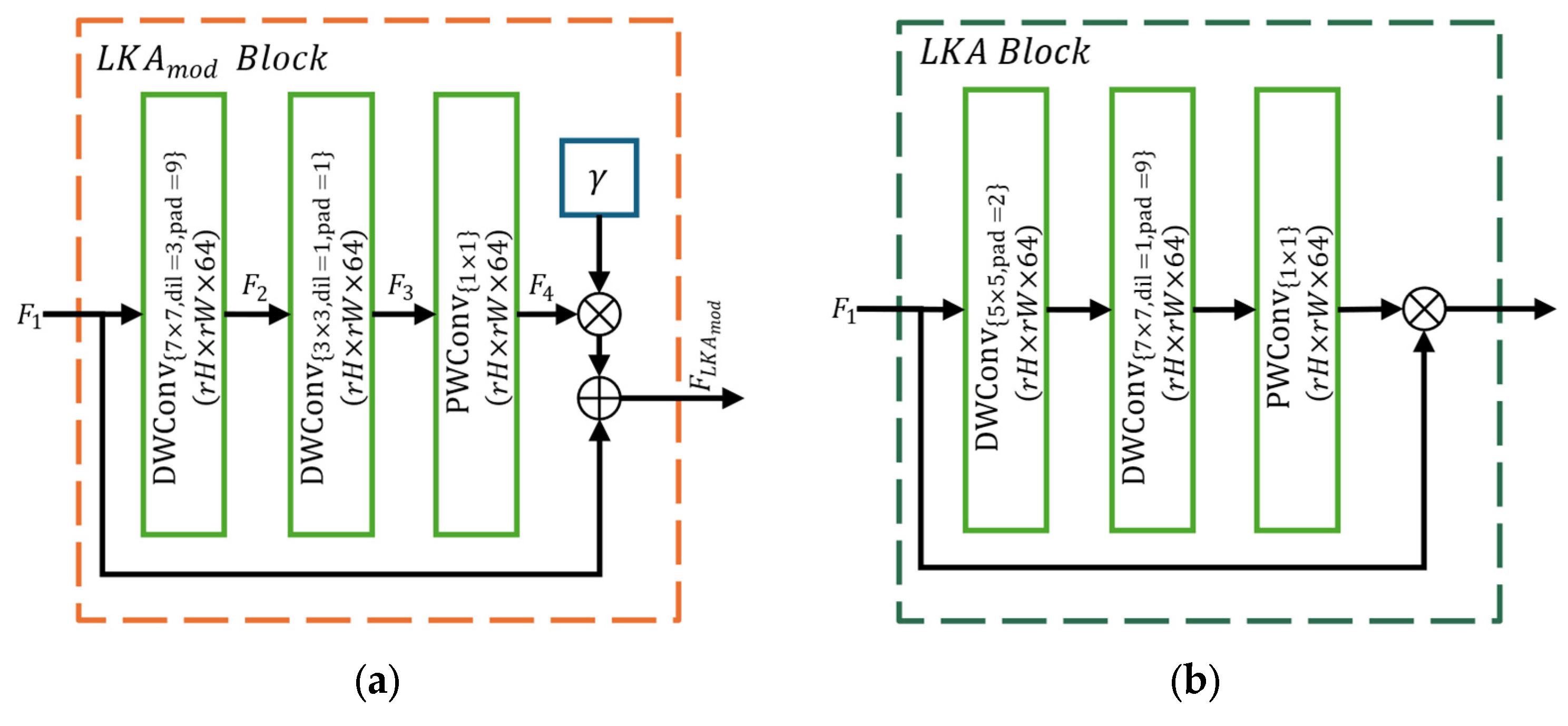
In this study, we propose an SR model based on residual neural networks, incorporating optimized attention modules to enhance the reconstruction of remote sensing images. Our method integrates a modified Large Kernel Attention (LKA) module to capture long-range spatial dependencies through dilated and grouped convolutions and an Optimized Convolutional Module (OCM) module to refine local contours and textures, thereby reducing information loss in high-frequency details. Additionally, the model utilizes a residual architecture with group normalization and skip connections, which enhances gradient propagation and ensures greater training stability.

The remainder of this document is structured as follows: Section 2 reviews related works, providing context and background on previous research. Section 3 describes the materials and methods employed in this study, beginning with an overview of the proposed approach and then including details about the network architecture. The results are subsequently presented in Section 4, with subsections dedicated to ablation tests and the performance of the proposed method using the Remote Sensing Super-Resolution Dataset (RRSSRD) [15]. Finally, Section 5 discusses the findings, followed by the conclusions in Section 6.

2. Related Works

In super-resolution, interpolation-based methods increase spatial resolution by estimating the missing pixels using the surrounding ones, as in the cases of bilinear, bicubic, and nearest-neighbor interpolation. However, these methods have significant limitations, resulting in smoothed images and the loss of high-frequency information details [16]. Due to the above, most SR methods for satellite images rely on reconstruction-based algorithms, such as those that incorporate sparse priors, which utilize prior knowledge to preserve structural details [17]. On the other hand, deep learning methods, particularly CNNs, have proven good fine detail reconstruction due to their focus on feature extraction through attention mechanisms.

2.1. Classical CNN-Based Methods

Classical super-resolution methods rely on standardized benchmark datasets such as Set5 and Set14 [9,17], which contain high-quality natural images captured under controlled conditions. These datasets do not adequately reflect the complexities inherent in remote sensing imagery, where factors such as atmospheric noise, illumination variations, and sensor calibration significantly affect the quality during acquisition. However, we address these benchmarks in this section for review purposes.

The principle of CNNs is to learn the mapping between LR and HR images in a supervised manner. Classical super-resolution methods include SRCNN, as proposed by Dong et al. [9], which demonstrates that CNNs are more effective for the SR process than traditional interpolation-based methods. Nevertheless, the shallow architecture of SRCNN, composed of only three convolutional layers, limits its ability to reconstruct complex details. Even so, the network achieved a Peak Signal-to-Noise Ratio (PSNR) of 36.66 dB on the Set5 dataset at a ×2 upscaling factor, demonstrating strong potential in simple configurations. Since SRCNN requires a pre-interpolation stage, the computational cost increases as the convolutional operations are performed on the upscaled image. To address these limitations, Dong et al. [18] implemented transposed convolutions in FSRCNN to reduce processing time by eliminating the need for pre-interpolation. Nonetheless, its performance remained limited in handling complex images and preserving spatial patterns. FSRCNN offered real-time inference speed and comparable PSNR to SRCNN but struggled with spatial complexity.

On the other hand, several studies have explored increasing network depth to enhance reconstruction performance. Kim et al. [10] proposed VDSR, a deep network that improved the quality of HR images by learning residuals directly between LR and HR, achieving significant improvements. This framework outperformed previous models by approximately 0.87 dB in PSNR on Set5 using a 20-layer architecture. Another deep architecture, EDSR, was developed by Lim et al. [11]. They modified the residual blocks to make them deeper and remove batch normalization, significantly improving the spatial quality in image reconstruction. EDSR achieved a PSNR of 38.20 dB on Set5 at ×2 upscaling factor and became a benchmark with over 43 million parameters. Similarly, another notable deep network is SRResNet, introduced by Ledig et al. [12]. This deep residual block-based network enables more efficient and artifact-free learning. Its main contribution was the integration of perceptual and adversarial losses, resulting in visually sharper images despite similar PSNR values to EDSR.

Although the above methods have been applied to natural images, remote sensing images still present challenges due to the noise introduced during acquisition. The results above show that increasing network depth and the number of parameters is directly related to PSNR improvements, enabling more accurate reconstruction of complex details. However, this improvement comes at the cost of increased computational load, which poses a disadvantage in hardware-constrained environments.

2.2. Attention-Based Architectures

Various strategies based on attention mechanisms have emerged to overcome the limitations of classical models in reconstructing fine details. These modules allow the network to focus its learning on relevant image features without excessively increasing network depth.

Zhang et al. [19] implemented a residual channel attention network (RCAN) to enhance SR performance, employing channel attention modules that prioritize local features. By incorporating channel attention (CA), the model applies inter-channel dependencies to assign adaptive weights, enhancing useful features while suppressing irrelevant information. RCAN achieved a PSNR of 38.27 dB on Set5 and surpassed EDSR while maintaining a similar depth. Lei et al. [20] proposed a local-global combined network (LGCNet), which integrates long-range information while prioritizing local details, thereby enabling better reconstruction through the inclusion of attention modules that focus on high-frequency regions and geographic patterns, making it particularly useful for satellite RGB images. This model enhanced urban feature recovery, though performance varied across test sets.

Salvetti et al. [8] proposed a model called RFANet for the SR of multiple remote sensing images by exploiting spatial and temporal correlations across multiple LR images through attention modules and 3D convolutions. This approach extracts relevant features and fuses data; however, in settings with only RGB satellite images, it lacks mechanisms to handle noise effectively, thus affecting reconstruction quality. Despite this, RFANet achieved improvements of over 1.2 dB in PSNR versus single-frame baselines. As a result, channel, spatial, and residual attention strategies have emerged. Guo et al. [21] introduced the concept of Large Kernel Attention (LKA), which captures large-scale spatial relationships without significantly increasing computational cost. However, careful hyperparameter tuning is required for each image type. LKA blocks demonstrate improved attention efficiency with PSNR gains of approximately 0.4 dB in natural images.

Hu et al. [22] oriented the attention process to the channel dimension through a squeeze-and-excitation (SE) operation that maps and condenses each channel’s features, followed by an excitation step where learned weights adjust the relevance of each channel. This approach prioritizes informative channels but lacks spatial attention, leading to detail loss. The SE block added minimal computational cost and has been adopted in various SR models with marginal accuracy gains. In contrast, Woo et al. [23] proposed a dual attention mechanism named CBAM, combining channel and spatial attention in a single block to focus on the most relevant features. However, it may present limitations when modeling long-range or global dependencies. CBAM was easy to integrate and showed approximately 0.2 dB gains in the previously mentioned SRResNet; however, it did not significantly improve the reconstruction of complex scenes.

More recently, transformer-based models have also shown promise in SR tasks. For instance, SwinIR [24] builds upon the Swin Transformer architecture [25] and introduces a modular design for image restoration. The model is composed of three main stages: a shallow feature extraction module that applies a convolutional layer to preserve low-frequency content; a deep feature extraction module that stacks residual Swin Transformer blocks to capture local dependencies and enhance features through self-attention and cross-window interactions; and finally, a reconstruction module that combines both shallow and deep features to produce high-quality HR images. This architecture achieves a balance between efficiency and performance, demonstrating strong results by leveraging both local attention mechanisms and residual learning strategies.

2.3. Noise and Degradation Handling

One of the main challenges in SR lies in accurately reconstructing LR images, as they not only suffer from a loss of structural information but also from noise contamination, which affects the overall image quality. For this reason, various denoising approaches have been explored within SR models to improve the recovery of textures and edges.

Zhang et al. [26] focus on noise suppression using the DnCNN architecture, which employs residual blocks with convolutions and batch normalization to model noise directly, proving effective across various levels of Gaussian noise. DnCNN outperformed BM3D and other traditional methods in the range of noise intensity η = 15 − 50. Nevertheless, its performance is limited when handling non-Gaussian noise or complex degradations.

Wu et al. [27] proposed DCANet for denoising under unknown noise distributions. This model is composed of the following components: a noise estimation network to identify noise characteristics, a spatial and channel attention module (SCAM) to highlight relevant features while suppressing irrelevant ones, and a dual convolutional structure that captures complementary information using dilated convolutions and residual connections, though it requires more careful hyperparameter tuning. DCANet achieved a Structural Similarity Index (SSIM) higher than 0.85 in real-world image datasets such as SIDD and demonstrated superior robustness under blind denoising scenarios.

Many of the aforementioned methods face the challenge of balancing model complexity with performance. Designing architectures that are both lightweight and capable of capturing the intricate details required for super-resolution remains a challenging task [28]. This limitation is particularly critical for remote sensing applications, where efficiently processing large-scale data is essential. Despite existing efforts, a need remains for strategies that effectively preserve reconstruction quality while significantly improving efficiency [29].

This work proposes a hybrid model called Optimized Attention Residual Network (OARN), which combines residual networks with visual attention blocks. The approach includes a module inspired by LKA [21] and another based on DCANet [27], both of which have been specifically modified and optimized for the SR task. This design enhances texture and contour reconstruction without significantly increasing computational complexity while preserving edges and texture information. The main contributions of the proposed method are described below:

• Enhanced reconstruction of edges and textures is achieved through a novel super-resolution system that introduces a modified Large Kernel Attention (LKA) block and an additional attention refinement module, specifically designed to improve spatial detail recovery;
• A balance between visual quality and computational efficiency is achieved through a reduced number of parameters and an optimized training strategy that enables rapid convergence without compromising accuracy;
• Validated robustness in recovering images from the same scene captured by different sensors using objective quality measures, such as PSNR, SSIM, Edge Preservation Index (EPI), and Perceptual Image Patch Similarity (LPIPS).

3. Materials and Methods

This section aims to provide a comprehensive description of all the components and processes involved in implementing and evaluating the proposed model. Accordingly, the proposed method is first introduced, highlighting the specific aspects of its architectural design and the elements required for its training. Next, the experimental setup used to evaluate the proposed approach is described, including the datasets and quality metrics employed in the assessment, as well as the details of the model’s hyperparameter optimization strategy.

3.1. Proposed Method

The designed system, illustrated in Figure 1 and referred to as OARN (Optimized Attention Residual Network), is developed to achieve high visual fidelity while maintaining a lightweight architecture, owing to the incorporation of attention mechanisms and optimized residual structures. Unlike VDSR [10], our proposal is divided into four main stages: Feature Map Extraction, LKA_mod block, OCM block, and residual blocks.

The LR image is converted from RGB to the YCbCr color space during the first stage. Subsequently, the luminance channel (Y) is passed through a convolutional layer to extract the initial features. These features are then processed by a modified LKA block designed to capture global information and enhance attention to key regions of the image without significantly increasing computational complexity. The third stage is the OCM block, which refines spatial details by applying additional convolutions to optimize reconstruction. In the fourth stage, the features pass through two convolutional blocks, integrating a skip residual connection that helps to preserve important information and improves training stability. Finally, a convolutional layer adjusts the output, which is then added to the original input image to produce the reconstructed Y output channel (Y_SR). This output is combined with the C_b and C_r chroma channels previously interpolated using bicubic interpolation. Finally, the resulting image is converted back to RGB color space, yielding an HR version with enhanced visual fidelity.

3.1.1. Feature Map Extraction

In the first step of the proposed method, the LR input image, which is in the $RGB$ color space, is converted to YC_bC_r as defined below:

$$\begin{gathered} I_{RGB}\in {\mathbb{R}}^{H\times W\times C}\to I_{YCbCr}\in {\mathbb{R}}^{H\times W\times 3},\mathrm{b}\mathrm{e}\mathrm{i}\mathrm{n}\mathrm{g} \\ Y\leftarrow 0.299·R+0.587·G+0.114·B, \\ {C}_r\leftarrow \left(R-Y\right)·0.713+\omega , \\ {C}_b\leftarrow \left(B-Y\right)·0.564+\omega , \end{gathered}$$

(1)

where $I_{RGB}\in {\mathbb{R}}^{H\times W\times 3}$ is the RGB LR image, with H denoting the image height, W the width, and C the number of channels. $I_{YCbCr}\in {\mathbb{R}}^{H\times W\times 3}$ represents the LR image in the YC_bC_r color space [30], where Y is the luminance channel, C_b is the blue-difference chroma component, $C_r$ is the red-difference chroma component, and w is defined as 128 for 8-bit images.

The Y channel is selected for processing by the model, as it contains most of the structural information while avoiding chromatic distortions. The Y_LR image is obtained by bicubic interpolation of Y and denoted as

$$Y_{LR}\in {\mathbb{R}}^{rH\times rW\times 1},$$

(2)

where H and W respectively represent the height and width of the image and r is a scaling factor. This representation is used as the input of the model to extract the initial feature map through a 3 × 3 convolution with padding of 1 pixel, which is represented as

$$F_1=\varphi \left({\mathrm{C}\mathrm{o}\mathrm{n}\mathrm{v}}_1\left(Y_{LR} \right)\right),$$

(3)

where ϕ(∙) represents the GELU (Gaussian Error Linear Unit) activation function [31].

This initial map, obtained using 640 trainable parameters, contains the primary representations that will be refined later through attention mechanisms and residual blocks.

3.1.2. Modified Large Kernel Attention (LKA_mod Block)

Spatial attention plays a fundamental role in SR, as it allows the enhancement of high-frequency information, improving edge preservation and optimizing the reconstruction of fine details. To achieve this, an optimized LKA block has been implemented, enabling the capture of global image information without significantly increasing computational cost.

The original LKA block [21] was designed to enhance the extraction of contextual features. Its architecture is based on a sequence of three convolutions that capture information at different scales before undergoing spatial refinement. As shown in Figure 2, the design employs a combination of depthwise and pointwise convolutions, effectively balancing computational complexity with the feature extraction process.

However, the original LKA design, illustrated in Figure 2b, presents specific limitations when applied to SR tasks. Although it effectively expands the receptive field, its reliance on large and dilated kernels may result in insufficient sensitivity to high-frequency textures, which are essential for reconstructing fine image details such as textures. Additionally, the final element-wise multiplication between the attention map and the input increases computational cost without delivering a substantial gain in reconstruction quality, a significant drawback in scenarios where visual fidelity must be achieved with limited computational resources.

To address this, the convolutional layers have been reorganized, as illustrated in Figure 2a. This modification enables more efficient capture of spatial context from the initial stages and allows for the extraction of refined features with reduced redundancy. By using depthwise separable convolutions, the number of operations and memory usage are significantly reduced. In particular, the proposed LKA_mod block decreases the number of parameters from 8832 in the original design to 8000, representing an approximate 9.42% reduction, without compromising the model’s ability to extract global spatial relationships or the quality of image reconstruction.

Given the spatial redundancies in satellite imagery, the exclusive use of standard convolutions can be suboptimal. In the modified version, as shown in Figure 2, separable convolutional layers are incorporated to reduce the number of operations while maintaining reconstruction quality.

The LKA_mod block takes the feature map from the initial convolution $\left(F_1\right)$ and transforms it as follows:

$$F_2=\mathrm{D}\mathrm{W}\mathrm{C}\mathrm{o}\mathrm{n}{\mathrm{v}}_{\left\{7\times 7,\mathrm{d}\mathrm{i}\mathrm{l}=3,\mathrm{p}\mathrm{a}\mathrm{d}=9\right\}}\left(F_1\right),$$

(4)

$$F_3={\mathrm{D}\mathrm{W}\mathrm{C}\mathrm{o}\mathrm{n}\mathrm{v}}_{\{3\times 3,\mathrm{d}\mathrm{i}\mathrm{l}=1,\mathrm{p}\mathrm{a}\mathrm{d}=1\}}\left(F_2\right),$$

(5)

$$F_4={\mathrm{P}\mathrm{W}\mathrm{C}\mathrm{o}\mathrm{n}\mathrm{v}}_{\{1\times 1\}}\left(F_3\right),$$

(6)

$${F_{LKA}}_{mod}=LK{A}_{mod}\left(F_1\right)=F_1+\gamma · F_4,$$

(7)

where $\gamma$ is a scaling factor, $\mathrm{D}\mathrm{W}\mathrm{C}\mathrm{o}\mathrm{n}\mathrm{v}$ stands for depthwise separable convolution. This kind of convolution allows an expanded receptive field without increasing the number of parameters. $\mathrm{P}\mathrm{W}\mathrm{C}\mathrm{o}\mathrm{n}\mathrm{v}$ refers to pointwise convolution, while dil specifies the dilation rate and pad indicates the padding size used in each convolution.

Unlike the original LKA design, where the output is multiplied by the input to recalibrate spatial features, in $LK{A}_{mod}$ the multiplication is omitted. Instead of multiplying the input as in the original design, the proposed block applies a scaled residual addition using the $\gamma$ factor, which is then summed with the original input. As a result, the number of operations is reduced by replacing costly multiplications with lighter-scaled additions. To determinate the optimal value of $\gamma$, preliminary tests were conducted with values of 0.001, 0.01, 0.1, and 1, training and validating the model for 20 epochs. These experiments showed stable converge from epoch 10, maintaining similar PSNR values (from 29.62 to 29.65 dB). Based on these preliminary results, $\gamma$ = 0.01 was selected as it provided the best balance between training stability and reconstruction quality. This approach subtly adjusts the spatial attention without oversaturating the initial feature map, stabilizes training, and reduces computational complexity while preserving the model’s ability to focus on relevant high-frequency regions.

3.1.3. Optimized Convolutional Module (OCM Block)

The OCM module is designed to refine the spatial features of the image, enhance the learned information, and improve the reconstruction of fine details. This module is based on the design of DCANet proposed by Wu et al. [27] but has been adapted for super-resolution tasks rather than denoising. While DCANet improves the quality of degraded images through two attention modules (spatial and channel), OCM focuses on preserving spatial details such as edges and textures while reconstructing high-resolution images. The OCM block diagram is presented in Figure 3.

The design of DCANet uses a dual architecture and various attention mechanisms. In contrast, OCM adopts the attention approach of DCANet but replaces dual attention with a spatial attention mechanism by implementing a modified version of the LKA block. This modification enhances the representation of high-frequency features without incurring additional computational costs. As a result, the module preserves robustness in high-frequency regions while maintaining structural information.

The complete process of the OCM module can be expressed mathematically as

$$F_5=\psi \left({\mathrm{C}\mathrm{o}\mathrm{n}\mathrm{v}}_5\left(F_{LK{A}_{mod}}\right)\right),$$

(8)

$$F_6=LK{A}_{mod}\left(F_5\right),$$

(9)

$$F_{OCM}=\psi \left({\mathrm{C}\mathrm{o}\mathrm{n}\mathrm{v}}_6\left(F_6\right)\right),$$

(10)

where ${\mathrm{C}\mathrm{o}\mathrm{n}\mathrm{v}}_5$ and ${\mathrm{C}\mathrm{o}\mathrm{n}\mathrm{v}}_6$ are $3\times 3$ convolutional layers with padding of 1 pixel, $\psi$ is the LeakyReLU activation function, and $LK{A}_{mod}$ represents the operations described in Equation (7). This structure of 81,856 trainable parameters ensures that attention is reinforced in relevant regions and that spatial information is efficiently refined, contributing to improved reconstruction quality.

3.1.4. Residual Blocks

The residual blocks shown in Figure 1 are based on the architecture proposed by Kim et al. [10] in the VDSR model. These blocks enhance reconstruction quality by focusing the learning process on the difference between the input image and the HR image rather than reconstructing the image from scratch. This learning is achieved by introducing a residual summation connection, which enables efficient gradient propagation during training, preventing the vanishing gradient problem while enhancing fine details and preserving edge structures.

Based on this architectural design, the proposed implementation reduces the number of residual blocks and introduces a skip connection after the OCM module. This connection is implemented using a 1 × 1 convolution, which serves as a linear projection to adjust dimensionality, enabling direct information flow across layers and improving training stability while maintaining computational efficiency.

After passing through the residual blocks and applying the residual addition with $Y_{LR}$, a final $3\times 3$ convolution is applied as a refinement layer to adjust the output, which is the reconstructed $Y$ channel $\left(Y_{SR}\right)$. The process is mathematically represented as follows:

$$F_7=\varphi \left(\mathrm{G}\mathrm{N}\left({\mathrm{C}\mathrm{o}\mathrm{n}\mathrm{v}}_7\left(F_{OCM}\right)\right)\right),$$

(11)

$$F_8=F_7+{\mathrm{C}\mathrm{o}\mathrm{n}\mathrm{v}}_8\left(F_{OCM}\right),$$

(12)

$$F_{Residual}=\varphi \left(\mathrm{G}\mathrm{N}\left({\mathrm{C}\mathrm{o}\mathrm{n}\mathrm{v}}_9\left(F_8\right)\right)\right),$$

(13)

$$Y_{SR}={\mathrm{C}\mathrm{o}\mathrm{n}\mathrm{v}}_{10}\left(Y_{LR}+F_{Residual}\right),$$

(14)

where $F_{OCM}$ is the output from the OCM module (see Equation (10)), ${\mathrm{C}\mathrm{o}\mathrm{n}\mathrm{v}}_8$ is a $1\times 1$ convolution, ${\mathrm{C}\mathrm{o}\mathrm{n}\mathrm{v}}_7$, ${\mathrm{C}\mathrm{o}\mathrm{n}\mathrm{v}}_9$ and ${\mathrm{C}\mathrm{o}\mathrm{n}\mathrm{v}}_{10}$ are $3\times 3$ convolutions with padding of 1 pixel, $\varphi$ represents the GELU activation function, $\mathrm{G}\mathrm{N}$ is a group normalization layer with 8 groups and 64 channels, and $Y_{SR}$ is the reconstructed $Y$ channel output. A point worth mentioning is that Equations (11)–(14) represent a block of 78,849 trainable parameters.

Finally, the output $Y_{SR}$ is combined with the chrominance components $C_b^{\prime }$ and $C_r^{\prime }$, which were previously interpolated using bicubic interpolation. To obtain the final high-resolution color image $I_{SR}$, the composite image is transformed from the $Y{C}_b{C}_r$ color space to RGB using the transform function $T_{Y{C}_b{C}_r\to RGB}$, defined as

$$\begin{gathered} I_{SR}=T_{Y{C}_b{C}_r\to RGB}\left(Y_{SR},C_b^{\prime },C_r^{\prime }\right), \\ R\leftarrow Y_{SR}+1.403·\left(C_r^{\prime }-\omega \right), \\ G\leftarrow Y_{SR}-0.714·\left(C_r^{\prime }-\omega \right)-0.344·\left(C_b^{\prime }-\omega \right), \\ B\leftarrow Y_{SR}+1.773·\left(C_b^{\prime }-\omega \right), \end{gathered}$$

(15)

where w is defined as 128 for 8-bit images.

3.2. Algorithm Summary

As described in the proposed method, the OARN model based on the VDSR architecture was optimized to achieve high visual fidelity without requiring deep networks. This is made possible through the implementation of efficient attention mechanisms and simplified residual blocks. The system consists of five main stages: (a) initial feature extraction, (b) spatial attention via $LK{A}_{mod}$, (c) spatial refinement using $OCM$, (d) residual processing via deep convolutions and skip connections, and (e) image reconstruction. The key modules optimizing the super-resolution process and their implementation are described below. Algorithm 1 presents the detailed steps involved in these processes.

Algorithm 1: OARN Super-Resolution Model

Input: Low-resolution RGB image IRGB

Output: Super-resolved image YSR

1. Initial Feature Extraction Input: IRGB Output: Feature map (F1) 1.1. Convert IRGB from RGB to YCbCr color space, as given in Equation (1). 1.2. ($Y_{LR},C_b^{\prime },C_r^{\prime })\leftarrow$ Bicubic interpolation of each channel in the YCbCr image using the scaling factor r. 1.3. F1 ← Convolution(YLR, kernel size = 3, padding = 1); use the YLR image defined in Equation (2). 2. Spatial Attention via LKAmod Input: F1 Output: Attention-enhanced feature map ($F_{LK{A}_{mod}}$) 2.1. F2 ← DepthwiseConv(F1, kernel size = 7, padding = 9, dilation = 3). 2.2. F3 ← DepthwiseConv(F2, kernel size = 3, padding = 1). 2.3. F4 ← Convolution(F3, kernel size = 1). 2.4. Compute $F_{LK{A}_{mod}}$ as in Equation (7). 3. Spatial Refinement with OCM Input: $F_{LK{A}_{mod}}$ Output: Optimized feature map (FOCM) 3.1. F5 ← Convolution($F_{LK{A}_{mod}},$ kernel size = 3, padding = 1, activation = LeakyReLU). 3.2. Compute F6 using the step 2 of this algorithm (Spatial Attention via LKAmod) with F5 as the input (see Equation (9)). 3.3. FOCM ← Convolution(F6, kernel size = 3, padding = 1, activation = LeakyReLU). 4. Residual Processing via Deep Convolutions and Skip Connections Input: FOCM Output: Residual Map FResidual 4.1. F7 ← GELU(GN(Convolution(FOCM, kernel size = 3, padding = 1), groups = 8)) as in Equation (11). 4.2. F8 ← F7 + Convolution(FOCM, kernel size = 1) 4.3. $F_{Residual} \leftarrow$ GELU(GN(Convolution($F_8$, kernel size = 3, padding = 1), groups = 8)). 5. Image Reconstruction Input: FResidual Output: SR image (ISR) 5.1. YSR ← Convolution(YSR + FResidual, kernel size = 3, padding = 1) 5.2. ISR ← Perform a color space transformation to RGB using the output of step 1.2 of this algorithm, as specified in Equation (15).

The proposed model can be trained using either of the following two loss functions. The L1 loss [32], also known as mean absolute error (MAE), is defined as the average of the absolute differences between the predicted output $I_{SR}$ and the ground truth $I_{HR}$:

$$L1=MAE={\displaystyle \frac{1}{N}}\sum _{i=1}^N\left|I_{SR}\left(i\right)-I_{HR}\left(i\right)\right|,$$

(16)

where |∙| denotes the absolute value operator, $I_{SR}\left(i\right)$ denotes the intensity of pixel $i$ in the SR image, $I_{HR}\left(i\right)$ represents the corresponding pixel intensity in the reference image, and $N$ is the total number of pixels. This function is less sensitive to outliers and favors edge preservation, making it useful for generating images with more defined details.

The L2 loss function, also known as the Mean Squared Error (MSE) [32], aims to minimize the difference between the reconstructed image $I_{SR}$ and the reference image $I_{HR}$, and it is defined as

$$L2=MSE={\displaystyle \frac{1}{N}}{\sum }_{i=1}^N{\left(I_{SR}\left(i\right)-I_{HR}\left(i\right)\right)}^2.$$

(17)

The choice between the L1 and L2 loss functions depends on the desired trade-off between robustness and sensitivity to large deviations in reconstruction. Both loss functions are evaluated in Section 4 to determine which one yields better reconstruction results in terms of visual quality and objective performance metrics.

3.3. Experimental Configuration

This section addresses the datasets and their preprocessing, as well as the metrics used to evaluate the proposed model. All experiments were conducted on a computing architecture with 32 GB of RAM, a 6-core AMD Ryzen 5 5600X processor, and an NVIDIA GeForce RTX 4070 Ti GPU. The programming environment was configured using Python 3.12.3, and the models were implemented in PyTorch 2.3.0.

3.3.1. Dataset and Preprocessing

The RRSSRD dataset was defined by Dong et al. [15] to evaluate their reference-based super-resolution method, which targets images captured at different time intervals using a more recent reference image, denoted as Ref image, that may not exactly represent the same scene as the target images. Although the proposed method is not reference-based, this study utilized the RRSSRD dataset to train and evaluate the model, as well as to conduct comparative analyses, since it includes representative remote sensing scenes captured by various sensors. The dataset comprises a training set of $4047$ image pairs consisting of HR and Ref images featuring scenes from Xiamen and Jinan, China, along with four test sets, each containing 40 pairs. Since the proposed approach does not use a reference image to compute the output, the Ref images were not utilized; only the HR images were used for training.

All the LR images were generated by applying bicubic downsampling with scale factors of 2, 3, and 4 to each HR image, thereby creating corresponding (LR, HR) image pairs for training. Additionally, each HR image was converted into the YCbCr color space. The luminance ($Y$) channel was normalized to the [0, 1] range, while the $C_b$ and $C_r$ channels were kept at their original range.

To increase the number of training samples without affecting the image information, a patch segmentation of 64 × 64 pixels with a stride of 41 pixels was applied. The HR images ($480\times 480$ pixels) and their corresponding LR versions were divided into patches. The remaining pixels were discarded to maintain a uniform patch size. This strategy increases data diversity while preserving spatial coherence and the integrity of visual information. Moreover, this technique enables the extraction of multiple meaningful regions from each image, improving the model’s learning efficiency. Additionally, data augmentation strategies were employed during training, including 90°, 180°, and 270° rotations, as well as horizontal and vertical flips, to enhance the model’s robustness. A point worth mentioning is that the training set was divided using the random split function of PyTorch’s utils module to obtain 20% of the samples for validation purposes and the remaining samples for training.

The assessment of OARN’s generalization capability was performed using the four test sets defined within the RRSSRD [15] dataset. Each one consists of 40 HR images from various sources, and their corresponding pairs were built following the previously indicated procedure.

Table 1. Description of the training and test subsets from the RRSSRD dataset.

Dataset	Number of Images	HR Image Source	Location	Resolution of HR Images
Training set	4047	Worldview-2, 2015 and GaoFen, 2018	Xiamen and Jinan, China	0.5 m–0.8 m
1st test set	40	Worldview-2, 2015	Xiamen, China	0.5 m
2nd test set	40	Microsoft Virtual Earth, 2018	Xiamen, China	0.5 m
3rd test set	40	GaoFen, 2018	Jinan, China	0.8 m
4th test set	40	Microsoft Virtual Earth, 2018	Jianan, China	0.5 m

presents a detailed description of each test set.

The diversity in the HR image sources allows the evaluation of variability across real-world scenarios and ensures the robustness of the model against different acquisition systems.

The WorldView-2 satellite [33] delivers high-resolution multispectral imagery, offering 0.5 m spatial resolution in panchromatic mode and 2 m in multispectral mode. It captures data across eight spectral bands, including the visible range 450–510 nm (blue), 510–580 nm (green), and 630–690 nm (red), as well as near-infrared bands, all with accurate radiometric calibration. The GaoFen-2 [34] satellite offers a spatial resolution of 1 m for panchromatic and 4 m for multispectral images, with bands centered at wavelengths similar to those of WorldView-2 but utilizing different sensor technologies, resulting in variations in spectral response, contrast, and sharpness. The dataset subset acquired from Microsoft Virtual Earth [35] provides RGB images with an approximate spatial resolution of 0.5 m. These images present higher variability in lighting and environmental conditions due to differences in acquisition time and atmospheric factors, thereby enriching the evaluation of the model under real-world variability.

The combination of these datasets enables the simulation of a non-uniform degradation scenario under realistic conditions. The diversity of image sources strengthens the model’s evaluation, particularly in remote sensing applications that involve data acquired from different sensors with their specific characteristics.

3.3.2. Evaluation Metrics

To qualitatively evaluate the experiments, three metrics commonly used in super-resolution tasks were employed to assess the effectiveness of the models.

PSNR [36] measures the quality of the reconstructed image by comparing it to the reference image in terms of MSE. It is defined as

$$PSNR=20{\log }_{10}\left({\displaystyle \frac{MA{X}_I}{\sqrt{MSE}}}\right) \mathrm{d}\mathrm{B},$$

(18)

where $MA{X}_I$ is the maximum possible pixel intensity value (255 for image in range [0–255]), and $MSE$ is the previously defined Mean Squared Error (see Equation (17)). Higher $PSNR$ values indicate better reconstruction quality.

SSIM [36] evaluates the similarity between the reconstructed and reference images in terms of luminance, contrast, and structure and is expressed as

$$SSIM\left(x,y\right)={\displaystyle \frac{\left(2{\mu }_x{\mu }_y+C_1\right)\left(2{\sigma }_{xy}+C_2\right)}{\left({\mu }_x^2+{\mu }_y^2+C_1\right)\left({\sigma }_x^2+{\sigma }_y^2+C_2\right)}},$$

(19)

where ${\mu }_x, {\mu }_y$ are the means of images $x$ and $y$, respectively. ${\sigma }_x^2,{\sigma }_y^2$ are their variances. ${\sigma }_{xy}$ is the covariance between the two images. $C_1=6.502 \mathrm{a}\mathrm{n}\mathrm{d} C_2=58.522$ are constants to avoid division by zero. $SSIM$ ranges from $0$ to $1$, where $1$ indicates perfect structural similarity with the reference image.

Edges represent important features in the images since visual perception and object recognition are based on their distribution. The Edge Preservation Index (EPI), proposed by Sattar et al. [37] and sometimes referred to as EC (Edge Correlation) [38], is a metric used to evaluate the effectiveness of a processing algorithm in preserving edges in an image [39,40]. EPI is defined as

$$EPI={\displaystyle \frac{\sum _{i=1}^N\nabla I_{SR}\left(i\right)·\nabla I_{HR}\left(i\right)}{\sqrt{{\sum _{i=1}^N\left(\nabla I_{SR}\left(i\right)\right)}^2}·\sqrt{{\sum _{i=1}^N\left(\nabla I_{HR}\left(i\right)\right)}^2}}},$$

(20)

where $\nabla I_{SR}\left(i\right)$ y $\nabla I_{HR}\left(i\right)$ represent the gradient at pixel $i$ in the super-resolved and reference images, respectively. The gradient was computed using the discrete Laplacian kernel $\left[\begin{array}{ccc}0& 1& 0\\ 1& -4& 1\\ 0& 1& 0\end{array}\right]$, which captures second-order spatial derivatives to emphasize sharp intensity variations, contributing to the identification of fine-grained details in the image.

This measure quantifies the extent to which edges are maintained after processing an image, with higher EPI values indicating better edge preservation. EPI is calculated by comparing the gradients (or differences in pixel values) in the original image and the processed image. Therefore, a higher EPI score indicates that the processing algorithm has performed better in preserving the sharp transitions in pixel values that define edges.

Additionally, the Learned Perceptual Image Patch Similarity (LPIPS) metric [41] was used for comparison with other models. LPIPS is a perceptual similarity measure that assesses the degree of similarity between two images from a human visual perception perspective. LPIPS compares deep features extracted from pre-trained Convolutional Neural Networks, capturing semantic and structural differences that align more closely with human judgment. A lower LPIPS score indicates greater perceptual similarity between the super-resolved image and the high-resolution reference. LPIPS is defined as

$$LPIPS\left(I_{SR},I_{HR}\right)={\sum }_l{\displaystyle \frac{1}{H_l{W}_l}}{\sum }_{h=l }^{H_l}{\sum }_{w=l}^{W_l}{‖w_l⨀\left({\varphi }_l{\left(I_{SR}\right)}_{h,w}-{\varphi }_l{\left(I_{HR}\right)}_{h,w}\right)‖}_2^2,$$

(21)

where ${\varphi }_l(·)$ denotes the activation map at layer $l$ of the pretrained network, $H_l$ and $W_l$ are the spatial dimensions at layer $l$, and $w_l$ are learned linear weights. The symbol $⨀$ represents element-wise multiplication.

4. Experimental Results and Discussion

This section presents the results of the experiments conducted to evaluate the effectiveness of the proposed OARN model. Various tests were performed using the RRSSRD dataset, with performance assessed through metrics such as PSNR, SSIM, and EPI, enabling the evaluation of both perceptual quality and structural fidelity of the generated images.

The analysis is organized into six subsections. Section 4.1 examines the effectiveness of attention modules using visual activation maps at various training epochs. Section 4.2 presents an ablation study to identify the contributions of the model’s key components. Section 4.3 investigates the impact of different optimizers and loss functions through a sensitivity analysis. Section 4.4 provides a comparative evaluation against state-of-the-art methods. Section 4.5 discusses qualitative visual results, and Section 4.6 summarizes the overall performance trends observed across all experimental settings.

4.1. Attention Module Effectiveness

To visually verify that the attention modules integrated into the proposed architecture are effectively learning relevant features, we applied LayerCAM [42] to multiple intermediate layers across different training epochs. In particular, we compare activations at epochs 5 and 60 for the OARN (AdamW + L1) model.

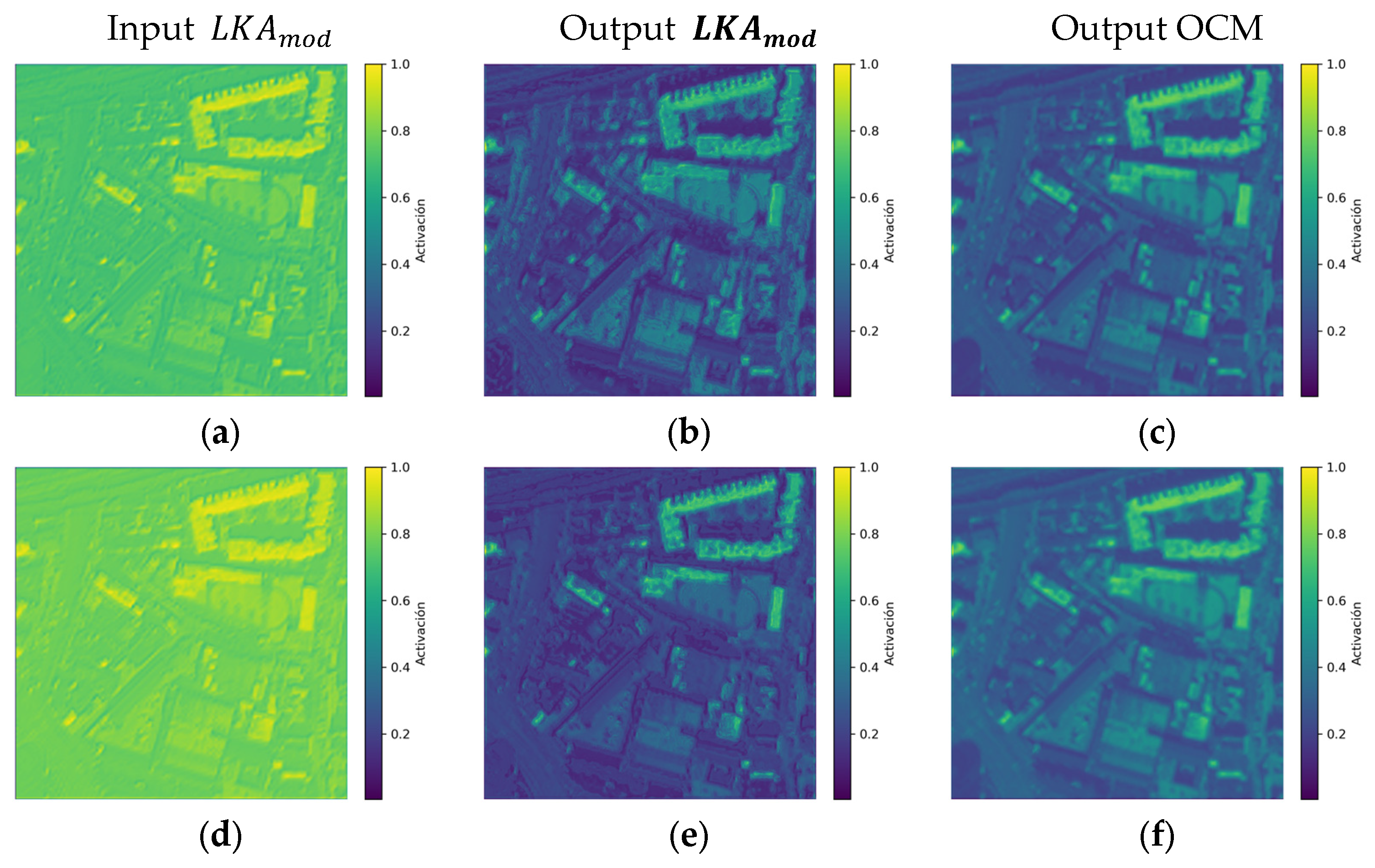
Figure 4 clearly illustrates how the activations of the attention modules evolve as the OARN (AdamW + L1) model is trained. At epoch 5, the output of the $LK{A}_{mod}$ module (Figure 4b) exhibits diffuse and less defined activations, indicating that the model is still in an early learning stage, without focused attention on relevant regions.

In contrast, at epoch 60, the output of the LKA_mod (Figure 4e) displays much more concentrated attention, where the activation maps clearly highlight the contours of buildings, roads, and other important geometric structures, demonstrating that the module progressively learns to identify relevant spatial patterns. Likewise, in the output of the OCM module (Figure 4f), the attention is focused on structurally and semantically valuable regions, such as street intersections and building edges, indicating that this module has improved its ability to direct attention to important elements in the image.

During the visual analysis conducted with LayerCAM on the activation maps generated at various stages of training, specific limitations in the performance of the proposed attention modules were identified. One of the main observations was that the model has difficulty distinguishing edges and relevant structures in images predominantly composed of green areas and mountainous regions. In such scenes, urban elements like rooftops, building contours, or roads are often partially obscured or softened by vegetation, making precise spatial detection more challenging. This issue particularly affects the LKA_mod module during early training stages.

At epoch 5, it was observed that in several cases, the $LK{A}_{mod}$ module failed to correctly distinguish contours or relevant structures when the buildings were surrounded by dense vegetation or when they consisted of large constructions with irregular or oval geometric shapes. The model’s learning improves significantly by epoch 60, and $LK{A}_{mod}$ exhibits more concentrated and effective attention over structurally significant regions. However, the OCM module was occasionally unable to adequately recover the information previously detected by $LK{A}_{mod}$, which limits the final refinement of features. Out of the 160 images analyzed, 47 cases at epoch 5 were identified where $LK{A}_{mod}$ and OCM jointly failed to recover the relevant regions of the image. At epoch 60, despite the LKA correctly identifying spatial patterns in most images, approximately 23 images were found in which the OCM module failed to reinforce or reconstruct the captured information effectively.

These limitations suggest that, although the proposed attention modules significantly improve the model’s performance in urban or structurally well-defined environments, their behavior may still be compromised in scenarios dominated by natural or homogeneous surroundings.

4.2. Ablation Test

To evaluate the impact of the different modules within the proposed model, an ablation study was conducted using the four test sets defined in Section 3.3.1, focusing on a $\times 4$ scaling factor, as it represents a more constrained scenario in terms of information recovery. Different model variants were trained and compared by removing or replacing key components such as LKA, OCM, DCANet [27], and the residual blocks, as well as testing alternative attention mechanisms like CBAM [23] and SE [22]. To ensure a fair evaluation, all variants were trained under the same configuration, using the L2 loss function defined in Equation (17) and the Stochastic Gradient Descent (SGD) optimizer (SGD + L2), both of which are widely adopted as a baseline setup in super-resolution tasks. The SGD optimizer was implemented with a learning rate of 0.0001, a momentum of 0.9 and a weight decay of $1\times {10}^{-4}$. Moreover, the batch size was set to 64, and the number of training epochs was set to 60.

Table 2. Ablation study: component configurations for each model variant. A “x” symbol indicates that the corresponding component is included in the model, whereas “-“ denotes exclusion.

Variant	LKAmod	LKAoriginal	OCM+	Residual
OARN (SGD + L2)	x	-	LKAmod	x
Modification 1	-	-	LKAmod	x
Modification 2	x	-	-	x
Modification 3	-	x	LKAoriginal	x
Modification 4	x	-	LKAmod	-
Modification 5	-	-	CBAM	x
Modification 6	-	-	SE + LKAmod	x
Modification 7	-	-	SE	x
Modification 8	-	-	DCANet	x

shows the configuration of the tested models. The first columns ($LK{A}_{mod}$ and $LK{A}_{original}$) indicate whether spatial attention mechanisms are present or absent before the OCM block. The OCM+ column specifies the attention mechanism integrated within the OCM block, replacing the $LK{A}_{mod}$ module indicated in Equation (9). The final column indicates whether residual blocks were retained within the OCM block.

Table 3. Average performance in PSNR, SSIM, and EPI under ×4 scale factor of each model variant across the four test sets.

Method	PSNR	SSIM	EPI
OARN (SGD + L2)	33.05	0.815	0.250
Modification 1	32.90	0.815	0.252
Modification 2	32.93	0.814	0.240
Modification 3	32.81	0.800	0.221
Modification 4	32.97	0.801	0.225
Modification 5	32.88	0.814	0.244
Modification 6	29.36	0.809	0.231
Modification 7	32.78	0.814	0.243
Modification 8	32.70	0.815	0.246

summarizes the average performance of all variants across the four test sets, using PSNR, SSIM, and EPI metrics, which reflects the robustness of the models when different acquisition sensors are employed. The results show that the OARN (SGD + L2) model achieves the best overall performance. The model incorporating the modified LKA module ($LK{A}_{mod})$ achieved superior performance across evaluation metrics, as evidenced by the comparison between OARN (SGD + L2) and variant Modification 3. Specifically, OARN (SGD + L2) outperformed Modification 3 by 0.01 in EPI, indicating improved edge preservation. Similarly, the variants in which the OCM and Residual modules were excluded (Modifications 2 and 4) obtained comparable but consistently lower results than the proposed method. Furthermore, the variants in which the $LK{A}_{mod}$ module is replaced (Modification 5–Modification 8) demonstrated reduced performance, with at least a 0.17 dB decrease in PSNR compared to the proposed approach.

Across all test sets, the proposed OARN (SGD + L2) model consistently outperformed its variants. The removal or replacement of attention modules resulted in the degradation of either structural quality or edge preservation, especially when spatial attention was removed. These results confirm the effectiveness of the proposed architecture, including the $LK{A}_{mod}$, OCM, and residual blocks.

To assess the statistical significance of the performance differences between the modifications and the base model OARN (SGD + L2), a paired t-test was conducted with a 95% confidence level, corresponding to a significance threshold of Bonferroni-corrected $p < 0.05/8 = 0.00625$. The test was performed across the four test sets, comprising a total of 160 image samples, resulting in 159 degrees of freedom. The results indicate that the performance gains of OARN (SGD + L2) are statistically significant and unlikely to have occurred by chance, with p-values below $8.70\times {10}^{-22}$ for PSNR, $5.98\times {10}^{-5}$ for EPI and $1.12\times {10}^{-7}$ for SSIM, except for Modification 8, where the p-value for SSIM was 0.08. This result suggests that Modification 8 does not significantly alter the global structure compared to OARN (SGD + L2). Nonetheless, OARN (SGD + L2) outperforms Modification 8 in the PSNR and EPI metrics.

4.3. Optimizer and Loss Function Selection

To evaluate the impact of the optimizer on the performance of the proposed OARN model, a sensitivity analysis was conducted using a scale factor of ×4. In this test, the SGD, Adam, AdamW, and Root Mean Square Propagation (RMSProp) optimizers were compared along with two widely used loss functions: L1 and L2.

The L2 loss function, defined in Equation (17), penalizes larger errors more heavily, often leading to smoother reconstructions but potentially over-smoothing high-frequency details. On the other hand, the L1 loss function, given in Equation (16), is often used in image reconstruction tasks.

The four optimizers were implemented using a learning rate of 0.0001. The SGD optimizer uses a momentum of 0.9 and a weight decay of $1\times {10}^{-4}$, the AdamW optimizer utilizes a weight decay of $1\times {10}^{-5}$ and the RMSprop optimizer employs $\alpha =0.99$. The remaining parameters were set to the default values provided by PyTorch’s optim module. The number of training epochs was set to 60, and a batch size of 64 was employed.

The results are presented in

Table 4. Average PSNR, SSIM, and EPI results across the four test sets using different combinations of optimizers and loss functions (L1 and L2) for scale factor ×4.

Method	PSNR	SSIM	EPI
SGD + L1	33.05	0.817	0.264
SGD + L2	33.05	0.815	0.250
Adam + L1	33.62	0.834	0.328
Adam + L2	33.46	0.828	0.308
AdamW + L1	33.66	0.836	0.333
AdamW + L2	33.62	0.837	0.334
RMSprop + L1	31.78	0.768	0.260
RMSprop + L2	32.14	0.789	0.281

, which displays the average values obtained across the four test sets described in Table 1. The results indicate that the AdamW + L1 combination was the most robust, achieving the highest average performance. Compared to the worst-performing configuration, RMSProp + L1, the AdamW + L1 setup achieved an improvement of $1.88$ dB in PSNR and $0.073$ dB in EPI, demonstrating better training capability and superior preservation of high-frequency details, as reflected in the EPI metric.

On the other hand, the Adam configurations also showed competitive results. For instance, Adam + L1 achieved an improvement of $0.57$ dB in PSNR compared to SGD + L2 and $0.16$ dB when compared to Adam + L2, suggesting a more accurate reconstruction of fine details. Nonetheless, the Adam + L1 configuration presents a slight decrement compared to its counterpart using AdamW.

To compare the impact of different optimizers and loss functions on model performance, statistical validation was conducted using a paired t-test with a 95% confidence level (Bonferroni-corrected $p < 0.05/7 = 0.007143$) on the 160 image samples of the test sets. The baseline configuration selected for comparison was the model trained with AdamW and L1 loss, due to its strong overall results. The results show that AdamW + L1 yields statistically significant improvements over the alternative settings, with observed p-values as low as $3.69\times {10}^{-38}$ for PSNR, $2.73\times {10}^{-7}$ for SSIM, and $1.64\times {10}^{-24}$ for EPI. An exception was found in the configuration using AdamW + L2, which yielded a p-value of 0.09 for EPI, suggesting no significant difference in that metric.

The training and validation curves for the four optimizers and the L1 and L2 loss functions are displayed in Figure 5a,b, allowing the observation of convergence stability and PSNR behavior on both training and validation sets throughout the epochs.

As observed in Figure 5a, the L1 loss combined with AdamW exhibits the highest PSNR values in both training and validation. On the other hand, RMSProp shows slower convergence with lower PSNR values and considerable instability, particularly in the validation curve. The Adam optimizer demonstrates performance similar to AdamW but with a lower PSNR in validation tests, while SGD displays slower convergence. Moreover, RMSProp exhibits poor stability in the validation data, indicating a reduced learning capacity. A point worth mentioning is that the combination of L2 loss with AdamW results in high and stable PSNR values during training. However, compared to the L1 loss function in Equation (16), the L2 loss in Equation (17) is generally slightly more computationally expensive. While this difference is often minimal in most scenarios, it becomes relevant when processing millions of samples or when models are deployed in resource-constrained embedded systems. In such contexts, L1 loss is preferable due to its lower computational overhead, making it a more suitable choice for remote sensing applications. Consequently, the model configured with AdamW and L1 loss was selected as the most appropriate baseline for comparing the proposed method against other state-of-the-art models.

4.4. Comparison with State-of-the-Art Methods

To evaluate the performance of the proposed OARN model, a direct comparison was conducted against several state-of-the-art super-resolution methods, including classical interpolation techniques (Bicubic), early CNN-based models (SRCNN [9] and VDSR [10]), and deeper residual architectures (EDSR [11], SRResNet [12], and SwinIR [24]). The evaluation was carried out on four independent test sets using three scale factors ($\times 2$, $\times 3$, and $\times 4$), and the results are summarized in Figure 6.

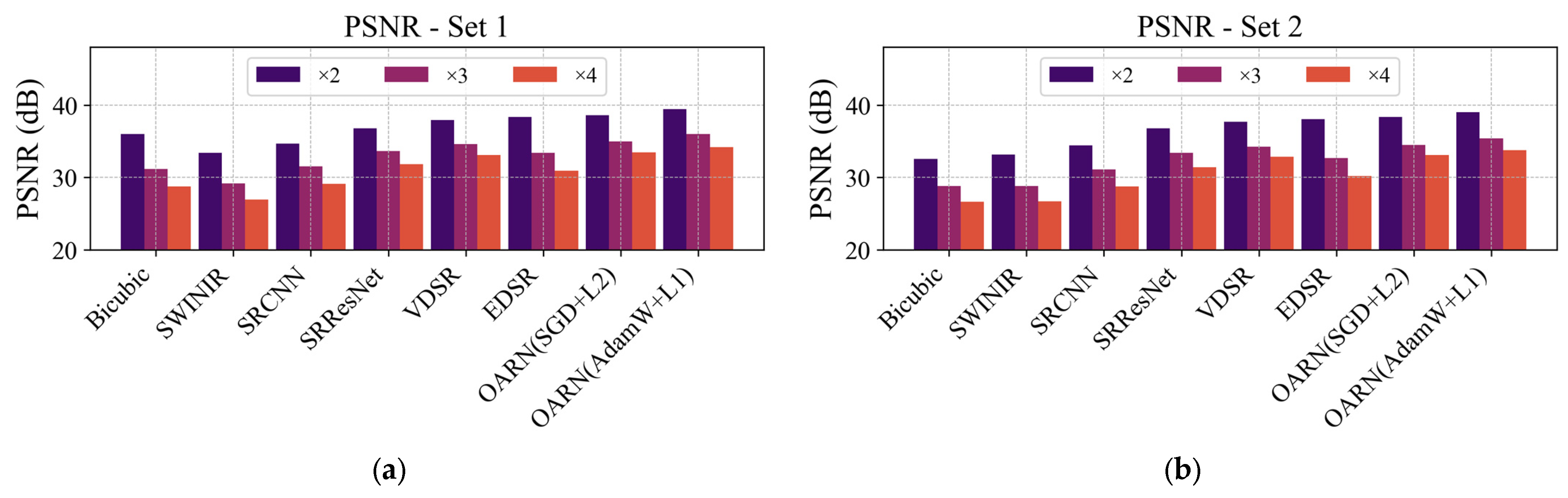
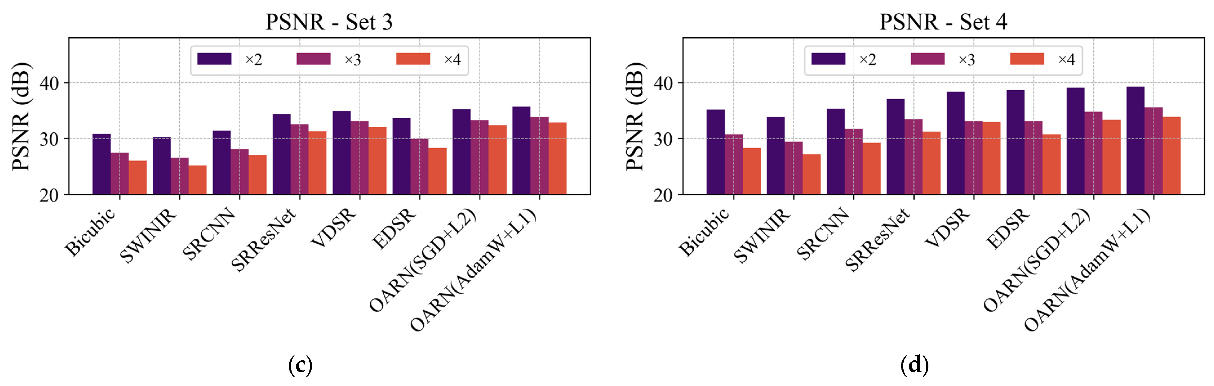
Figure 6 shows that the OARN model consistently outperforms comparative methods in terms of PSNR across all test sets and scale factors. The OARN (AdamW + L1) configuration achieved the highest average PSNR in all scenarios, reaching up to $39.44$ dB at scale $\times 2$ (Figure 5a), $35.98$ dB at $\times 3$, and $34.18$ dB at $\times 4$, even surpassing deeper models such as EDSR, whose maximum was 38.37 dB at $\times 2$.

Compared to VDSR, OARN (AdamW + L1) showed an average improvement of over $1.1$ dB across all test sets at scale $\times 4$, demonstrating superior capability in recovering fine structures under conditions of spatial information loss. Similarly, concerning SRResNet, OARN achieved gains ranging from $1.4$ to $2.6$ dB, highlighting its efficiency without requiring an excessively deep network.

In contrast, SwinIR demonstrated lower performance than convolution-based models, such as VDSR and EDSR, across all sets and scales, as Swin Transformer blocks require longer training to effectively capture high-frequency textures.

Test set 1, composed of HR images acquired with the WorldView-2 satellite, showed that the OARN model achieved the highest PSNR values among all methods, particularly for the ×2 and ×3 scaling factors, demonstrating the model’s ability to leverage spatial information effectively. In test sets 2 and 4, which include images from Microsoft Virtual Earth, improvements were also observed despite variations in lighting and environmental conditions. In contrast, test set 3, which is based on images from the GaoFen-2 satellite with a resolution of 0.8 m per pixel, exhibited lower PSNR values, indicating that the OARN model struggled to recover details when the spatial resolution was more limited. Although this ground sampling distance is relatively close to that of WorldView-2 and Microsoft Virtual Earth datasets (0.5 m), the difference in native spatial resolution significantly impacts the quality of fine detail reconstruction, which contributes to the lower quantitative results observed in this case. Nevertheless, the proposed model still achieved PSNR values above 30 dB, demonstrating acceptable reconstruction quality under these more challenging conditions.

These results validate the robustness of the proposed approach, showing that OARN achieves a competitive balance between reconstruction quality and computational efficiency, outperforming state-of-the-art methods across multiple test scenarios.

4.5. Qualitative Analysis

The quantitative analysis shown in Figure 6 demonstrates that the proposed model, OARN (AdamW + L1), achieves the highest PSNR values across all test sets and scale factors. To complement these results, a comparative qualitative analysis was conducted using reconstructed images from test sets 3, 1, and 2, evaluated at a $\times 4$ scale factor. These scenes are presented in Figure 7, Figure 8 and Figure 9, respectively, and were selected due to their high complexity and rich textures. They include elements such as buildings, trees, and roads, which introduce numerous edges and fine structural details. Such characteristics pose greater challenges for SR models, making them ideal for visually assessing the model’s ability to preserve details and accurately reconstruct complex patterns. To visually assess the differences in reconstruction quality, error maps were generated for each of the compared methods. These maps were obtained by computing the inverse absolute difference between the original HR image and its corresponding reconstruction in the cropped region. The error was normalized between 0 and 1 and subsequently inverted to highlight more accurate regions in lighter tones. The visualization corresponds to the average absolute error across the three RGB channels, multiplied by 255 for display in greyscale.

In Figure 7, corresponding to test set 3, it can be observed that the OARN (AdamW + L1) model presents a more uniform and clearer error map compared to the other methods. Although EDSR achieves a more detailed reconstruction of edges, its PSNR is lower by 5.92 dB, which is attributed to the presence of artifacts and inconsistencies in more complex regions.

Although EDSR generates visually sharp images and achieves high EPI values, its low PSNR score suggests notable discrepancies in pixel-wise intensity values. In other words, while the reconstructed images appear visually coherent in terms of color and structure, the pixels’ intensities deviate more significantly from the ground truth. This behavior could be attributed to the model overfitting on global structures, potentially at the expense of accurately capturing fine-grained local details. Furthermore, OARN (AdamW + L1) achieves the lowest MSE (46.71) and MAE (5.45) scores, indicating a closer match to the ground truth at the pixel level. In contrast, SwinIR exhibits the worst performance, with the lowest PSNR (22.76) and the highest MSE (355.15) and MAE (18.84), indicating significant distortions in pixel intensity. Similarly, although EDSR obtains a lower LPIPS value than OARN (0.279 vs. 0.308), suggesting better perceptual similarity from a human perspective, its MSE (182.67) and MAE (10.78) scores indicate lower fidelity to the original image in terms of pixel-level accuracy.

In Figure 8, OARN (AdamW + L1) preserves cylindrical structures and geometric details, while methods such as VDSR and SRResNet display irregular edges and darker error maps in high-frequency regions. Although SRResNet achieves competitive metrics, it tends to alter colors and lose texture in complex areas, as reflected in its higher MSE (51.96) and MAE (5.75) compared to OARN’s lower MSE (32.95) and MAE (4.57). In terms of perceptual quality, OARN also achieves a lower LPIPS score (0.146) than SRResNet (0.283), indicating a better perceptual similarity to the ground truth. On the other hand, EDSR achieved a slightly higher EPI score (0.474) compared to OARN (0.441), suggesting marginally better edge preservation. Nevertheless, OARN (AdamW + L1) produced a more consistent error map and a cleaner reconstruction, demonstrating a balance between structural fidelity and computational efficiency with a significantly lighter architecture. In contrast, SwinIR recorded the highest errors in all three metrics (MSE = 237.56, MAE = 15.41, and LPIPS = 0.369), revealing substantial perceptual and numerical distortions.

Finally, in Figure 9, corresponding to an urban scene with buildings and complex infrastructure, OARN (AdamW + L1) exhibits sharper and more continuous recovery of building and road contours. In contrast, SRCNN and VDSR produce irregular lines and less-defined edges, as evidenced by both the reconstructions and the error maps. Although EDSR slightly outperforms OARN (AdamW + L1) in EPI (0.390 vs. 0.388), as in the previous case, this marginal difference is offset by a cleaner and more consistent visual output produced by the proposed model. Furthermore, OARN (AdamW + L1) achieves a higher PSNR, reinforcing its ability to maintain an appropriate balance between visual accuracy and structural preservation, particularly in images acquired from the Microsoft Virtual Earth dataset. Additionally, it obtains the lowest MSE (43.17) and MAE (5.24), as well as a relatively low LPIPS value (0.191), indicating high pixel-wise and perceptual similarity to the ground truth. In contrast, SwinIR presents the highest MSE (315.40), MAE (17.75), and LPIPS (0.387), confirming significant perceptual and structural degradation.

As shown in Figure 7, Figure 8 and Figure 9, EDSR generates images with well-defined edges and continuous structures; however, it introduces slight inconsistencies in intensity values, particularly in textured areas, which affects the PSNR. These results suggest that EDSR tends to overfit to high-level structural patterns, potentially compromising pixel-wise accuracy. While the model may produce perceptually coherent reconstructions, it does so at the cost of precise alignment with ground truth at the pixel level. In contrast, OARN achieves a balanced performance in both PSNR and EPI, producing homogeneous error maps and reconstructions that are closer to the actual pixel values.

4.6. Training Time and Computational Efficiency Analysis

The results discussed in the previous sections demonstrate that OARN (AdamW + L1) not only achieves the highest PSNR and EPI values across multiple test sets and scales but also preserves both structural and perceptual quality, even in scenes acquired from different sensors with varying characteristics. These improvements are evident considering the model’s computational efficiency.

Table 5. Comparison of computational efficiency, training time, and inference speed across different super-resolution methods.

Method	Parameters	GFlops			Total Training Time (s)	Average Inference Time (s)	Estimated RAM Usage (MB)
		×2	×3	×4
SRCNN	8129	0.430	0.184	0.100	3289	0.0004	9.82
SwinIR	11,900,199	677.58	306.10	178.20	15,451	0.0938	7133.76
VDSR	664,704	38.287	17.016	9.571	101,987	0.0020	142.91
SRResNet	1,546,880	128.010	56.893	32.002	129,157	0.0170	926.12
EDSR	43,061,760	2890.034	1284.459	722.508	235,680	0.0472	2710.47
OARN (AdamW + L1)	169,345	9.73	4.33	2.43	48,505	0.0011	104.07

presents a comparative analysis of the computational efficiency of the proposed OARN (AdamW + L1) model against other state-of-the-art super-resolution methods. The evaluation includes the number of parameters, floating-point operations (GFlops), total training time, and average inference time per image. RAM consumption was measured using the torchinfo library [43], with an input size of 120 × 120 pixels to generate a SR output of 480 × 480 pixels, which represents a ×4 scale.

The OARN (AdamW + L1) method features a reduced number of parameters (169,345) and exhibits a low computational cost across all scale factors, with 9.73 GFlops at scale $\times 2$, 4.33 GFlops at scale $\times 3$, and 2.43 GFlops at scale $\times 4$, making it highly efficient for multiscale scenarios. Despite its compact design, the approach achieves competitive performance due to its optimized architecture.

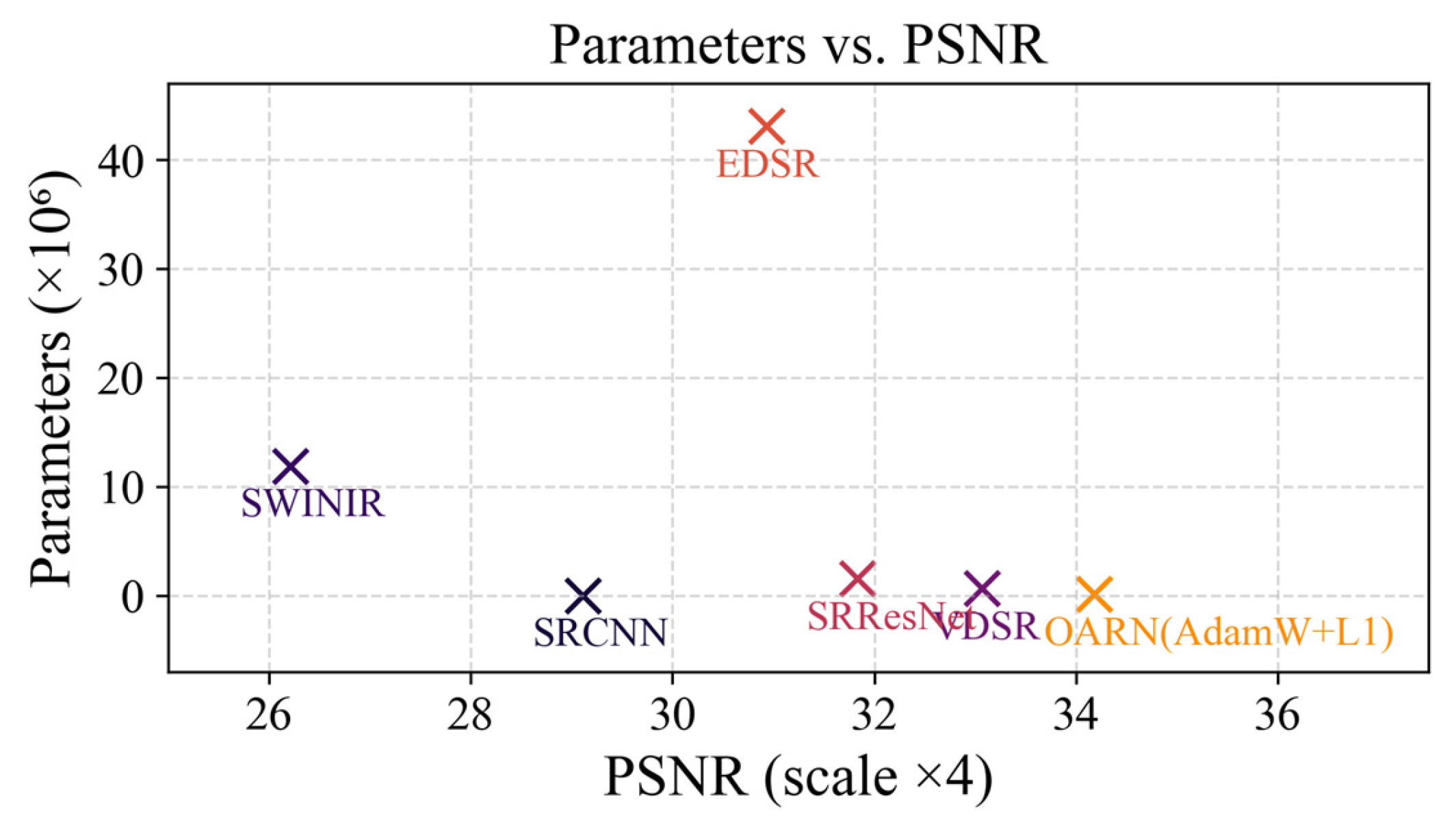
Although the proposed method has a higher number of parameters compared to SRCNN, which exhibits low computational complexity with only 8129 parameters and significantly lower reconstruction quality, the scatter plot in Figure 10 shows that OARN (AdamW + L1) achieves a higher PSNR while using considerably fewer parameters than deeper models such as EDSR. Therefore, although the proposed method involves greater complexity than some simpler models, it achieves a more efficient balance between quality and computational cost, making it a better overall alternative.

In comparison, EDSR exhibits a computational load of 722.508 GFlops at $\times 4$ scale. This indicates that OARN (AdamW + L1) reduces operations by approximately 99%, requiring around 297 times fewer operations to reconstruct at the same scale.

Even against intermediate models such as SRResNet, which reaches 32.002 GFlops at $\times 4$ scale, OARN (AdamW + L1) achieves a reduction of $92\%$ in computational cost, offering better efficiency while consuming fewer computational resources.

Moreover, the SwinIR model exhibits high computational complexity, with 11.9 million parameters and a GFLOPs count that exceeds OARN’s across all three scales, being 73 times higher at ×4 scale.

Regarding inference time, the proposed OARN (AdamW + L1) method achieved an inference time of $0.0011$ s, representing $98\%$ improvement compared to EDSR, which takes $0.0472$ s per image.

OARN (AdamW + L1) demonstrates a significant improvement over SRResNet, which requires $0.0170$ s, resulting in approximately 94% reduction in time. Even compared to VDSR, the proposed model is $45\%$ faster. Although the SRCNN model achieves an inference time of $0.0004$ s, it exhibits significantly lower reconstruction quality. Therefore, OARN offers a better balance between reconstruction quality and inference efficiency.

SwinIR, in contrast, requires 0.0938 s per image, making it the slowest among all evaluated models and highlighting its limited practicality in real-time applications. In terms of estimated RAM usage, SwinIR consumes the highest amount at 7133.76 MB, followed by EDSR with 2710.47 MB and SRResNet with 926.12 MB.

OARN (AdamW + L1) achieves one of the lowest RAM usages with only 104.07 MB, which demonstrates that it performs better in memory-constrained environments without compromising accuracy. In comparison, VDSR uses 142.91 MB, while SRCNN has the lowest footprint at 9.82 MB, albeit with significantly poorer reconstruction quality.

As shown in Figure 10, the OARN (AdamW + L1) model achieves the highest PSNR value (34.18 dB) at the ×4 scale reconstruction with only 169,345 parameters. In contrast, EDSR requires over 43 million parameters while obtaining a lower PSNR (30.93 dB). This demonstrates that greater model complexity does not necessarily guarantee better reconstruction quality. Similarly, SRResNet and VDSR achieve PSNR values of 31.83 dB and 33.07 dB with 1.54 million and 0.66 million parameters, respectively, showing significantly lower performance compared to OARN (AdamW + L1). SwinIR, despite its complex transformer-based design with over 11 million parameters, achieves a PSNR of only 26.49 dB, further validating that architectural size does not imply better quality.

This indicates that the proposed model strikes a balance between efficiency and quality, achieving the highest PSNR with a considerably more compact architecture than other state-of-the-art methods, thereby validating its effectiveness in terms of both accuracy and resource utilization.

5. Discussion

The experimental results demonstrate that the OARN model is highly effective for the task of SR in satellite imagery. The proposed architecture, which integrates the $LK{A}_{mod}$ block and the OCM module, achieves significant improvements in reconstructing structural and textural details, outperforming both traditional and state-of-the-art methods in terms of PSNR, SSIM, and EPI. These enhancements are achieved without resorting to very deep networks or incurring excessive computational costs.

One of the main advantages of OARN lies in its efficient design. With only 169,345 parameters and a computational cost of 2.43 GFLOPs at scale $\times 4$, the model remains lightweight while achieving superior performance. In contrast, EDSR requires over 43 million parameters and 722.508 GFLOPs to perform at a lower quality level, indicating that higher complexity does not necessarily translate into better results. The trade-off between quality and the computational burden is clearly favorable for OARN, as shown in Figure 10, where it achieves the highest PSNR with a considerably smaller model.

The $LK{A}_{mod}$ block enables the capture of long-range spatial dependencies, while the OCM module refines local features such as edges and textures, thereby enhancing image fidelity. In addition, the optimized residual blocks promote gradient flow and training stability while facilitating the learning of residual differences between LR and HR images.

Another major contribution of this study is the model’s robustness across multisensory-acquired datasets. OARN was evaluated on four independent test sets, including imagery from WorldView-2, GaoFen-2, and Microsoft Virtual Earth, each with distinct spatial resolutions and spectral properties. The model consistently delivered competitive results across all sets, particularly in structurally complex scenes. For instance, in test set 3 (GaoFen-2), where spatial degradation poses a challenge, OARN maintained high PSNR and EPI values. Meanwhile, in test set 1 (WorldView-2), it demonstrated its ability to fully exploit fine spatial information.

Moreover, the proposed method operates solely on the intensity channel, which makes its extension to multispectral or hyperspectral images a promising direction for future work. Since the chroma channels ($C_b$ and $C_r$) are processed using a conventional bicubic upsampling strategy, the core architecture remains independent of color-specific operations and could be adapted to handle other spectral bands similarly. However, the current implementation relies exclusively on RGB input data, which limits the exploitation of additional spectral information available in richer imaging modalities. While this simplifies the model design and training, it also restricts its applicability in domains where non-visible bands (e.g., infrared) carry essential information.

Nonetheless, some limitations remain. While the $LK{A}_{mod}$ and OCM modules significantly improve spatial attention and texture preservation, their performance depends on the careful tuning of hyperparameters and kernel configurations. The ablation study revealed that removing or replacing these components with alternatives, such as SE or CBAM, can result in performance drops of up to 3.69 dB in PSNR and 0.019 in EPI. These results highlight the importance of these modules but also suggest room for further optimization. In addition, as discussed in Section 4.1, the model showed decreased effectiveness in more homogeneous or natural environments, where structural information is less prominent. This behavior suggests that the proposed attention modules may have limited capacity to generalize across diverse landscape types. Future work may explore the integration of hybrid attention mechanisms that simultaneously leverage spatial and spectral features, further enhancing the model’s generalization capability and resilience in real-world remote sensing scenarios.

6. Conclusions

This study proposed the OARN framework, a novel residual architecture for single-image super-resolution in remote sensing. The model integrates two key components: the $LK{A}_{mod}$ and OCM blocks, which together improve spatial and perceptual reconstruction while maintaining computational efficiency. Trained and validated on the RRSSRD dataset, OARN demonstrated superior performance in objective metrics, including PSNR, SSIM, EPI, and LPIPS, as well as in subjective visual quality when compared to state-of-the-art methods. The ablation study confirmed the contribution of both $LK{A}_{mod}$ and OCM components, as their removal or replacement resulted in significant performance drops. Furthermore, OARN reduced the number of operations by up to approximately 99% compared to EDSR and achieved faster inference times than SRResNet, VDSR, and EDSR, indicating its potential for real-time deployment. Although the model’s performance is sensitive to hyperparameter settings and may degrade under severe noise or distortion, future work will explore the integration of adaptive and lightweight attention mechanisms to increase robustness in challenging remote sensing scenarios.