Enhancing Radial Distribution System Performance Through Optimal Allocation and Sizing of Photovoltaic and Wind Turbine Distribution Generation Units with Rüppell’s Fox Optimizer

Abstract

Renewable energy sources are being progressively incorporated into modern power grids to increase sustainability, stability, and resilience. To ensure that residential, commercial, and industrial customers have a dependable and efficient power supply, the transmission system must deliver electricity to end-users via the distribution network. To improve the performance of the distribution system, this study employs distributed generator (DG) units and focuses on determining their optimal placement, sizing, and power factor. A novel metaheuristic algorithm, referred to as Rüppell’s fox optimizer (RFO), is proposed to address this optimization problem under various scenarios. In the first scenario, where the DG operates at unity power factor, it is modeled as a photovoltaic system. In the second and third scenarios, the DG is modeled as a wind turbine system with fixed and optimal power factors, respectively. The performance of the proposed RFO algorithm is benchmarked against five well-known metaheuristic techniques to validate its effectiveness and competitiveness. Simulations are conducted on the IEEE 33-bus and IEEE 69-bus radial distribution test systems to demonstrate the applicability and robustness of the proposed approach.

1. Introduction

The electric power system is traditionally divided into three main components: generation, transmission, and distribution [1,2]. Among these, the distribution system serves as the final stage in delivering electrical energy to consumers and is considered one of the most critical and complex segments of the grid. It is responsible for stepping down the voltage and distributing power to residential, commercial, and industrial users. However, the distribution network often encounters several operational and technical challenges, including voltage instability, significant power losses, and poor voltage profiles, which are primarily attributed to the high resistance-to-reactance (R/X) ratio characteristic of distribution feeders [3].

These problems make the system less efficient and reliable, and they also complicate its ability to meet modern energy needs and handle decentralized energy sources [4]. Numerous optimization and control strategies have been proposed in the literature to address these problems. These include network reconfiguration, which involves altering the topology of the distribution network to minimize losses and improve load balancing [5,6,7]; optimal capacitor placement, which enhances voltage profiles and reduces reactive power flow [8]; and the integration of distributed generation (DG) units [9], which are typically small-scale, decentralized energy sources such as photovoltaic (PV) systems, wind turbines (WTs), or microturbines. DG units strategically located near load centers can inject both active and reactive power into the grid [10], thereby reducing the stress on centralized power plants and transmission infrastructure. The implementation of Flexible AC Transmission System (FACTS) devices has received interest due to their ability to manage power flows dynamically, regulate voltage levels, and enhance the overall stability and adaptability of the distribution system [11].

Optimizing the placement and sizing of DG units in power distribution networks is crucial due to the increasing adoption of renewable energy and the growing demand for greater efficiency. Traditional optimization methods have demonstrated limitations in addressing the non-linear, multi-constrained nature of DG allocation problems. Research typically categorizes solution approaches into analytical methods, metaheuristic algorithms, and hybrid techniques that integrate sensitivity analysis with metaheuristics. Each offers specific advantages in minimizing power losses, reducing voltage deviations, and enhancing reliability and economic performance [12,13,14].

Analytical methods form the foundation for determining the optimal placement and sizing of DG, utilizing mathematical models and deterministic algorithms to deliver efficient solutions. They provide precise results under defined conditions, and recent advances have enhanced their ability to handle increasingly complex network scenarios [13,14]. Sensitivity-based approaches analyze how variations in generation or load affect system performance, helping identify optimal DG locations. By calculating sensitivity indices, these methods estimate the impact of small changes in DG placement and sizing on losses, voltage profiles, and other key metrics [12,15,16].

Among these, metaheuristic techniques have gained significant attention due to their flexibility and effectiveness in handling complex, non-linear optimization problems encountered in DG planning.

In [15], the authors combined a sensitivity index method with the Artificial Gorilla Troops Optimizer (AGTO) to optimally place biomass-based DG units in radial distribution systems. Their hybrid approach significantly improved voltage stability and reduced power losses, outperforming traditional methods, such as Grey Wolf Optimization (GWO). In [17], Non-dominated Sorting Genetic Algorithm-II (NSGA-II) combined with Linear Programming (LP) was used to optimally allocate and dispatch Battery Energy Storage Systems (BESS) in a high level of PV installations distribution network. The approach, enhanced by K-means clustering of annual load and generation profiles, significantly improved voltage regulation, reduced daily energy losses by up to $9.6\%$, and lowered peak demand by more than $20\%$. In [18], the authors applied Genetic Algorithm (GA), Particle Swarm Optimization (PSO), and Salp Swarm Algorithm (SSA) to determine the optimal location and size of BESS in high-DG penetration networks, where the DGs comprise PVs and WTs. Their results showed that PSO and SSA effectively minimized system cost, reduced power losses, improved voltage profiles, and mitigated reverse power flow, with PSO generally delivering the best overall performance. In [19], a hybrid algorithm combining Artificial Rabbits Optimization (ARO) with quasi-opposition-based learning and a novel line stability index was proposed for optimal placement of PV and BESS. Applied to the IEEE 33-bus system, it achieved a power loss reduction of up to $92.6\%$ and a nearly $100\%$ improvement in voltage deviation, demonstrating strong performance in both single-objective and multi-objective optimization. In [20], a hybrid approach combining Loss Sensitivity Factor (LSF) and Dwarf Mongoose Optimization (DMO) was developed to determine the optimal location and sizing of DG and DSTATCOM. Applied to radial distribution systems, the method demonstrated notable improvements in power loss reduction, voltage profile, and operational cost, outperforming several existing algorithms, including the Dragonfly Algorithm (DA), Shell Game Optimization (SGO), and SSA.

In [21], the authors introduce a Chaotic Quasi-Oppositional Arithmetic Optimization Algorithm (CQOAOA) for the optimal placement and sizing of solar and wind distributed generators in radial distribution networks. The method aims to reduce power loss, minimize emissions, and decrease operating costs, and has been proven on 33-bus and 94-bus systems (Portuguese system). The CQOAOA achieved improvements of 58.69%, 99.94%, and 22.30% for power loss, emissions, and cost, respectively, in the 33-bus system, and 77.81%, 99.98%, and 21.44% in the 94-bus system. The use of chaotic maps and quasi-oppositional learning improves convergence and solution quality in multi-objective optimization. In [12], the Osprey Optimization Algorithm (OOA) is employed to tackle the issues of DG placement and sizing in radial distribution networks. The focus of the study is on reducing real power losses by the incorporation of Type I (solar photovoltaic) and Type III (wind turbine) DGs. The OOA is tested on IEEE 33-bus, 118-bus, and a real-time Malaysian 54-bus system, achieving power loss reductions of 52.47% (Type I) and 71.95% (Type III) in the 33-bus system, and 72.56% (Type I) and 94.88% (Type III) in the Malaysian 54-bus system. This approach improves minimum bus voltages and surpasses several contemporary optimization strategies, showcasing its efficacy and versatility for practical distributed generation integration. In [22], the Teaching–Learning-Based Optimization (TLBO) method is employed to determine the appropriate location and sizing of photovoltaic-based DG and DSTATCOM units inside a radial distribution network. The approach accounts for uncertainties in load demand and PV generation using stochastic programming and Monte Carlo simulation, evaluating scenarios with varying degrees of certainty. Implemented on the IEEE 33-bus test system, the method achieves a 94.8% reduction in power losses and a 36.8% improvement in voltage stability index (VSI), reaching 0.9745 p.u. The inclusion of both active and reactive power injection from PV-DG and DSTATCOM enhances system performance. At the same time, comparative analysis confirms the superiority of TLBO in terms of solution quality and computational efficiency. In [12], the authors present a hybrid method combining the Active Power Loss Sensitivity (APLS) index with a Modified Ant Lion Optimization (MALO) algorithm for optimal placement and sizing of PV and wind turbine DGs. Applied to IEEE 69-bus, 85-bus, and 118-bus systems, the approach minimizes power losses and voltage deviation, achieving up to 96.10% loss reduction with wind turbine and 68.67% with PV in the 69-bus system. The MALO algorithm, enhanced with Lévy flights, improves solution quality and convergence. A comparative analysis confirms the method’s superiority over the Ant Lion Optimization (ALO), Bat, and Artificial Bee Colony (ABC) algorithms.

Other studies have employed various metaheuristic algorithms to determine the optimal location and size of installed DGs, including PSO [23], a Modified PSO algorithm (MPSO) [24], Multi-Objective Grey Wolf Optimization (MOGWO) [25], Modified Fitness-Dependent Optimizer (MFDO) [26], AGTO [27], Tasmanian Devil Optimization (TDO) [27], GWO [28], hybrid GWO-PSO [29], Garra Rufa Optimization (GRO) [30], Dingo Optimization Algorithm (DOA) [31], Battle Royal Optimization (BRO) [32], ABC [33], Moth-Flame Optimizer (MFO) [34], an Improved Whale Optimization Algorithm (IWOA) [35], Harris Hawks Optimization (HHO) [36,37], and Rider Optimization Algorithm (ROA) [38].

Most of these studies aim to minimize active power losses and reduce voltage deviation, using the location and size of the installed DGs as decision variables, typically assuming a constant power factor. The objective of this paper is to apply a newly proposed metaheuristic algorithm, namely Rüppell’s fox optimizer (RFO), under different DG-type scenarios, alongside RIME algorithm [39], electric eel foraging optimization (EEFO) [40], Whale Optimization Algorithm (WOA) [41], GA [42], and Sine Cosine Algorithm (SCA) [43]. In one of these scenarios, the power factor is also considered as a decision variable, alongside the installed active power and the locations of the DGs, to minimize total active power losses and voltage deviation. The IEEE 33-bus and 69-bus systems are used as benchmark systems in this study.

The remainder of this paper is organized as follows. Section 2 presents the problem formulation, including the objective function and constraints for installing DG in the distribution system. Section 3 introduces RFO and details its mathematical model. Section 4 discusses the results, highlighting the optimal location and sizing of DG units under various scenarios using the RFO applied to the IEEE 33-bus and 69-bus distribution systems. Finally, Section 5 concludes the paper with a summary of the key findings and future directions.

2. Problem Formulation

2.1. Modeling of Distribution Generation Units

Distributed generation refers to small-scale generators installed near load centers, capable of injecting both active and reactive power into the network. DG can be categorized based on the type of power it generates or consumes [44], as follows:

• Type 1 generates only active power, such as PV systems.
• Type 2 delivers active and reactive power, such as WTs.
• Type 3 provides only reactive power, such as synchronous condensers.
• Type 4 generates active power but consumes reactive power, as in induction generators.

This study focuses exclusively on Type 1 and Type 2 DG. Specifically, Type 1 is considered to be solar PV-based DG (PVDG), while Type 2 refers to WT-based DG (WTDG).

A standard solar PV system supplies real power to a radial distribution power network. The output power, denoted as $P_{pv}$, depends on environmental conditions, particularly solar irradiance and temperature. The output power of the PV system is mathematically expressed in (1) [12,45]

$$P_{pv}=\left\{\begin{array}{cc}{P}_{pvr}\times \left({\displaystyle \frac{G}{G_r}}\right),\hfill & 0<G<G_r\hfill \\ P_{pvr},\hfill & G\ge G_r\hfill \end{array}\right.$$

(1)

where $P_{pvr}$ denotes the rated output power of the solar PV units; G represents the solar irradiance at the selected location (in W/m²); and $G_r$ is the rated solar irradiance at the Earth’s surface (also in W/m²).

The active power ($P_W$) and reactive power ($Q_W$) outputs of a WT system are modeled in (2) and (3), respectively. The active power output is given by [12,45]

$$P_W=\left\{\begin{array}{cc}0,\hfill & 0\le v\le v_{cin}\mathrm{or}v\ge v_{cout}\hfill \\ P_{wr}\times \left({\displaystyle \frac{v-v_{cin}}{v_r-v_{cin}}}\right),\hfill & v_{cin}<v<v_r\hfill \\ P_{wr},\hfill & v_r\le v\le v_{cout}\hfill \end{array}\right.$$

(2)

In this equation, $P_{wr}$ represents the rated output power of the WT at its rated wind speed; v and $v_r$ are the actual and rated wind speeds at the selected location, respectively; and $v_{cin}$ and $v_{cout}$ denote the cut-in and cut-out wind speeds.

This study analyzes the load flow in a distribution system integrated with distributed generation using a suitable DG modeling approach. DG units can be modeled as either constant active and reactive power sources (PQ model) or constant active power and voltage sources (PV model).

In this work, the PVDG is modeled as a constant active power source. Similarly, WTs operating with a fixed power factor ($PF$) or controlling reactive power locally are modeled as constant PQ sources. The reactive power $Q_W$ of the WT is given by

$$Q_W=P_W\sqrt{{\displaystyle \frac{1}{P{F}^2}}-1}$$

(3)

The integration of PVDG and WTDG requires the installation of additional components, such as monitoring systems and power converters. While power electronic converters can introduce harmonics [46], the PVDG and WTDG themselves are not the source of these harmonics; by using well-designed converters and control techniques, the harmonics percentage can be reduced [47,48,49]. Therefore, this study treats the integrated DG and its associated components as a source of pure sinusoidal voltage waveforms.

Let $P_{Li}$ and $Q_{Li}$ represent the active and reactive power the load absorbs at bus i before DG integration. After integrating DG, the active and reactive power absorbed at bus i are expressed as

$$P_{nLi}=P_{Li}-P_{DG}$$

(4)

$$Q_{nLi}=Q_{Li}-Q_{DG}$$

(5)

where $P_{nLi}$ and $Q_{nLi}$ denote the new active and reactive powers consumed at bus i. The terms $P_{DG}$ and $Q_{DG}$ represent the active and reactive power of the DG, respectively. For a solar photovoltaic system, $Q_{DG}=0$, resulting in $PF=1$.

2.2. Forward/Backward Sweep Power Flow Analysis

Load flow analysis determines key network parameters using only the power injected or consumed at each node. While traditionally applied in transmission systems for tasks like generation scheduling, it is increasingly valuable in distribution networks for load control, network reconfiguration, DG integration, and electric vehicle planning. Standard methods include Gauss–Seidel, Newton–Raphson, and fast-decoupled approaches.

Unlike transmission systems, distribution networks exhibit high R/X ratios, radial structures, numerous nodes, and frequent topology changes resulting from maintenance or emergencies. These characteristics make traditional Jacobian-based load flow methods (like Newton–Raphson, Gauss–Seidel, and fast-decoupled) ineffective or computationally intensive. Even with improvements to the Newton–Raphson method, execution time remains a concern despite enhanced robustness. Numerous studies have highlighted the limitations of Jacobian-based methods for distribution systems, noting that transmission-oriented load flow techniques are inadequate for practical distribution challenges. As a result, many researchers favor the backward/forward sweep approach.

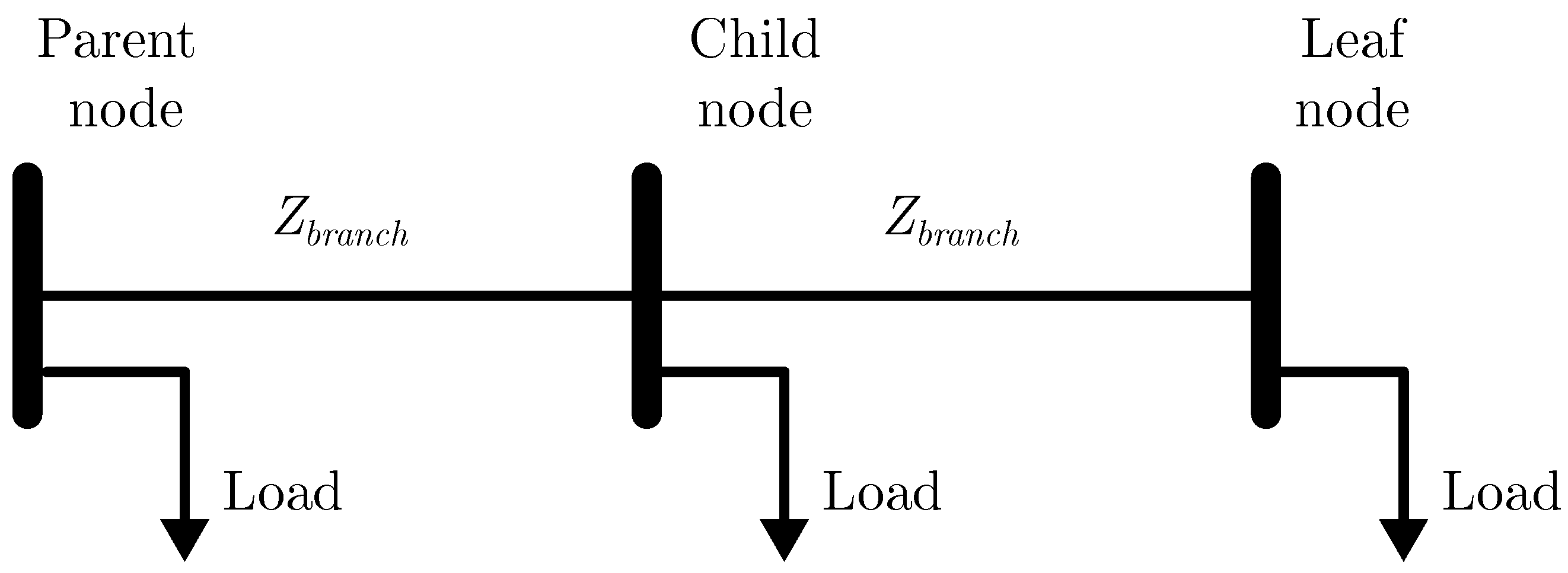
The backward/forward sweep approach is based on three main steps, considering a sample distribution system as shown in Figure 1. The following steps are formulated.

Figure 1. A simple radial distribution network.

Step 01 (nodal current calculation): the current injection at each node “i” is calculated using the following equation:

$$J_i^{(k+1)}={\left({\displaystyle \frac{S_i}{V_i^{\left(k\right)}}}\right)}^{\ast }-Y_i{V}_i^{\left(k\right)}$$

(6)

where $J_i^{(k+1)}$ is the current injected into node i in iteration $(k+1)$, $V_i^{\left(k\right)}$ is the voltage at node i in iteration k, $S_i$ is the complex power injection at node i, and $Y_i$ is shunt admittance at node i.

Step 02 (backward sweep): starting from the leaf nodes (end nodes) and moving toward the source, compute branch currents recursively. The sum of all currents injecting to branch i is calculated as follow:

$$I_i^{(k+1)}=J_i^{(k+1)}+\sum _{j\in C_i}{I}_j^{(k+1)}$$

(7)

where $I_i^{(k+1)}$ is the current flowing through branch i in iteration $(k+1)$, $I_j^{(k+1)}$ the current of branch j in $(k+1)$-th iteration, and $C_i$ is the set of child branches directly connected downstream to branch i.

The equation enforces Kirchhoff’s Current Law (KCL): Branch current = injected current at node i + sum of downstream branch currents.

Step 03 (forward sweep): starting from the source node (root) and moving toward the end nodes, update node voltages using Ohm’s Law.

$$V_j^{(k+1)}=V_i^{(k+1)}-I_j^{(k+1)}\times Z_j$$

(8)

where $Z_j$ impedance of the branch connecting parent node i to child node j, $V_i^{(k+1)}$ at parent node i in $(k+1)$-th iteration, and $V_j^{(k+1)}$ voltage at child node j in $(k+1)$-th iteration.

After each iteration, verify if the voltages have stabilized: ${max}_i\left|\left|V_i^{k+1}\right|-\left|V_i^k\right|\right|\le \epsilon$, where $\epsilon$ is the tolerance limit. If satisfied, terminate; otherwise, repeat Steps 1–3.

2.3. Objective Function

This paper aims to minimize total power loss, enhance the voltage profile by reducing voltage deviations, and ensure compliance with system constraints.

The primary objective of installing PVDG and WTDG in the distribution system is to minimize active power losses while maintaining voltage levels within permissible limits. However, improper placement or sizing of PVDG and WTDG can cause significant issues across the entire power system. Therefore, determining the optimal location and size of DG is formulated as a multi-objective optimization problem.

The multi-objective function comprises two main components related to total active power losses $f_1$ and voltage deviation $f_2$.

The function related to the total active power loss $f_1$ is defined as

$$f_1={\displaystyle \frac{TP{L}_{DG}}{TPL}}$$

(9)

where $TP{L}_{DG}$ represents the total active power losses after DG installation, while $TPL$ denotes the total active power losses before DG installation. For many studies in radial distribution systems (such as the IEEE 33- or 69-bus systems), a common formulation for the total active power losses is based on the sum of the losses in each branch. In its simplest form, the loss in a branch connecting buses i and j is given by

$$P_{loss}=\sum _{i,j\in N_{bus}}{\displaystyle \frac{(P_{ij}^2+Q_{ij}^2)}{V_i^2}}{R}_{ij}$$

(10)

In many papers, the “exact loss” expression is presented in a more general (often double summation) form:

$$P_{loss}=\sum _{i=1}^{N_{bus}}\sum _{j=1}^{N_{bus}}\left[{\alpha }_{ij}(P_i{P}_j+Q_i{Q}_j)+{\beta }_{ij}(P_i{Q}_j-P_j{Q}_i)\right]$$

(11)

where $N_{bus}$ is the total bus number, and $Z_{ij}=r_{ij}+j{x}_{ij}$ are the $ij$-th element of $Z_{bus}$, with coefficients:

$${\alpha }_{ij}={\displaystyle \frac{r_{ij}}{V_i{V}_j}}cos({\delta }_i-{\delta }_j),{\beta }_{ij}={\displaystyle \frac{r_{ij}}{V_i{V}_j}}sin({\delta }_i-{\delta }_j)$$

where $P_i$ and $Q_i$ are the net injections at bus i, and $V_i$ and ${\delta }_i$ are its voltage magnitude and phase angle. Both formulations ((10) and (11)) are used in DG placement and sizing studies, but for systems such as IEEE 33- or IEEE 69- bus, the branch loss formula of (10) is especially popular because it fits naturally with the backward/forward sweep methods typically used for load flow in radial networks.

The voltage deviation $f_2$ is defined as

$$f_2=\sum _{i=1}^{N_{bus}}{(1-V_i)}^2\times 100$$

(12)

To simplify the optimization problem, the multi-objective function is transformed into a single-objective function ($OF$) using the weighted sum method, as follows:

$$OF={\omega }_1{f}_1+{\omega }_2{f}_2$$

(13)

where ${\omega }_i$ is the weighted coefficient, with $\sum {\omega }_i=1$.

2.4. System Constraints

Both industrial and residential consumers are impacted by the power quality in distribution systems, which has a significant effect on the performance of connected loads. This is especially important in industries where technological equipment and production processes are highly susceptible to power supply fluctuations. Serious problems with the power system may arise if the parameters of the power distribution system are not kept within specific acceptable ranges. The operational limits of distribution networks following DG installation are defined by these ranges, which are frequently referred to as the system’s physical boundaries and operational constraints. These conditions are as follows.

Bus voltage limits: This involves ensuring the power quality of distribution networks necessitates voltage constraints. When the node’s supply voltage exceeds the allowable working range, electrical devices may experience malfunctions or failures. Consequently, it is imperative to effectively monitor and implement the voltage restrictions specified below throughout distribution networks.

$$V_{min}\le V_i\le V_{max}$$

(14)

where the minimum and maximum voltage limits are denoted by $V_{min}=0.95$ pu and $V_{max}=1.05$ pu, respectively.

The branch current limits: This is when each power line includes a defined load-carrying capability dictated by its material composition and cross-sectional area. Surpassing this capacity may activate protection relays, interrupt the power supply, or inflict physical damage to the line structure, leading to financial losses [50]. Consequently, establishing a maximum permissible current for each electrical line is crucial to ensure its safe operation. The following inequality constraint represents this limit:

$$I_k\le I_{max,k}k=1,2,\dots N_B.$$

(15)

where $I_{max,k}$ is the maximum current at the k-th branch, $N_B$ is the total branches number, and $I_k$ is the current of the k-th branch.

DG active and reactive power limits: DGs can generate active and reactive power within their specified characteristics. Therefore, each DG must be constrained by its maximum and minimum allowable active and reactive power, as defined by the following constraints:

$$P_{min}\le P_{DGi}\le P_{max}$$

(16)

$$Q_{min}\le Q_{DGi}\le Q_{max}$$

(17)

where $P_{min}$ and $Q_{min}$ are the minimum active and reactive power, $P_{max}$ and $Q_{max}$ are the maximum active and reactive power, and $P_{DGi}$ and $Q_{DGi}$ are the rated active and reactive power of the i-th DG, respectively.

Total DG active and reactive power limits: DGs inject active and reactive power at the nodes of distribution networks to decrease the power supplied by the source at the slack node. This injection also reduces power losses and voltage deviation in the distribution system, with higher DG capacity leading to greater loss reduction. However, the total injected power of all DGs is constrained by turbulence and instability that occur when certain limits are exceeded, as follows:

$$\sum _{i=1}^{nbDG}{P}_{DGi}\le \sum P_d$$

(18)

$$\sum _{i=1}^{nbDG}{Q}_{DGi}\le \sum Q_d$$

(19)

where $nbDG$ is the total number of installed DGs, and $P_d$ and $Q_d$ are the total demanded active and reactive powers, respectively.

The power balance constraint: This constraint ensures that the total generated active and reactive power in the distribution network, including power generated by DGs, matches the total system demand and associated losses. Mathematically, this is expressed through (20) and (21).

$$P_g+\sum _{i=1}^{nbDG}{P}_{DGi}=\sum P_d+TP{L}_{DG}$$

(20)

$$Q_g+\sum _{i=1}^{nbDG}{Q}_{DGi}=\sum Q_d+TQ{L}_{DG}$$

(21)

The first equation accounts for the active power, where the sum of the active power generated by the primary grid $P_g$ and all DG units (${\sum }_{i=1}^{nbDG}{P}_{DGi}$) must equal the total active power demand $\sum P_d$ plus the total active power losses in the network due to the integration of DGs $TP{L}_{DG}$. Similarly, the second equation ensures reactive power balance, where the combined reactive power generation from the grid and DG units must match the total reactive demand and the reactive power losses $TQ{L}_{DG}$. These constraints are critical to maintaining system stability, voltage regulation, and ensuring reliable operation of the distribution network, especially when optimally siting and sizing DG units.

The DG location constraint: DG units must not be installed on the same bus. Additionally, DGs may be placed on any bus within the system except for the slack bus.

The power factor constraint: The power factor of each DG unit must remain within the following range:

$$P{F}_{min}<P{F}_{DGi}\le P{F}_{max}$$

(22)

where $P{F}_{DGi}$ denotes the power factor of the i-th DG unit, $P{F}_{min}$ is the minimum allowable power factor, and $P{F}_{max}$ is the maximum allowable power factor.

The percentage reduction in total power losses can be determined using the following equations:

$$P_{red}={\displaystyle \frac{|TPL-TP{L}_{DG}|}{TPL}}\times 100$$

(23)

$$Q_{red}={\displaystyle \frac{|TQL-TQ{L}_{DG}|}{TQL}}\times 100$$

(24)

where $TQL$ and $TQ{L}_{DG}$ denote the total reactive power losses before and after the integration of DG, respectively.

3. Rüppell’s Fox Optimizer

Rüppell’s fox optimizer (RFO) was proposed in [51], and the inspiration for RFO is from the adaptive and collective behavior of Rüppell’s foxes. These desert-dwelling animals exhibit remarkable flexibility, thriving in a wide range of environments and adjusting their diet according to seasonal food availability. Rüppell’s fox inspired the creation of a metaheuristic that mimics their resourceful and flexible way of solving problems by using their opportunistic foraging strategies, social nature, and ability to work together in challenging situations. The RFO can be modeled mathematically as in the following sections.

3.1. Initialization of RFO

The algorithm begins by generating random solutions to address the relevant optimization problem. These solutions can be represented by a 2D array as follows:

$$y=\left[\begin{array}{cccc}{y}_1^1& y_2^1& \dots & y_d^1\\ y_1^2& y_2^2& \dots & y_d^2\\ ⋮& ⋮& \ddots & ⋮\\ y_1^n& y_2^n& \dots & y_d^n\end{array}\right]$$

(25)

where n is the population size, d is the number of decision variables, and $y_d^i$ represents the position of the i-th Rüppell’s fox in the d-th dimension.

The initial population is defined as

$$y_j^j=L_j+r(U_j-L_j),i=1,2,\dots ,N,j=1,2,\dots ,D$$

(26)

where $y_i^j$ is the value of the j-th decision variable for the i-th Rüppell’s fox, $L_j$ and $U_j$ represent the lower and upper bounds of the j-th decision variable, respectively, and r is a uniformly distributed random number in the range $(0,1)$.

3.2. Searching for Prey in Daylight

The senses of sight and hearing are represented by the variables s and h, as defined in Equations (27) and (28), respectively. Under the condition $(p-0.5)\ge 0$, $s\ge h$, and $rand\ge 0.25$, the search based on sight is governed by Equation (29). Here, $p\in [0,1]$ is a random variable that toggles between day and night states, and $rand$ is a uniformly distributed random number in the interval $\left[0,1\right]$.

$$s={\displaystyle \frac{1}{1+exp\left((K/2-k)/100\right)}}$$

(27)

$$h={\displaystyle \frac{1}{1+exp\left((k-K/2)/100\right)}}$$

(28)

$$y_{k+1}^i=x_k^i+r_{\mathrm{index}}(x_{\mathrm{rand}}-x_k^i)+r_{\mathrm{index}}(f_{{\mathrm{best}}_k}-x_k^i)$$

(29)

where k and K denote the current and the maximum number of iterations, respectively. The variable $y_{k+1}^i$ represents the position of the i-th Ruppell’s fox at iteration $(k+1)$, while $x_k^i$ indicates its position at iteration k. The term $f_{\mathrm{best}k}$ refers to the best global position identified by any Ruppell’s fox up to iteration k. Additionally, $r_{\mathrm{index}}$ and $x_{\mathrm{rand}}$ are specified in Equations (30) and (31), respectively.

$$r_{\mathrm{index}}=floor\left(4\times ran{d}_1+1\right)ran{d}_2$$

(30)

$$x_{\mathrm{rand}}=lbes{t}_k^i\left(Q\right)$$

(31)

where $ran{d}_1$ and $ran{d}_2$ are uniformly distributed random numbers within the interval $[0,1]$. The term $lbes{t}_k^i\left(Q\right)$ represents the i-th best-known position vector, recognized by Rüppell’s fox population at iteration k, where Q indicates that the optimal position is reached randomly, as described in (32).

$$Q=ceil\left(n·rand(1,n)\right)$$

(32)

where $rand(1,n)$ denotes a vector of length n, containing random values uniformly distributed in the range $[0,1]$.

Rüppell’s foxes are capable of detecting food sources within a field of view exceeding $260°$ due to the rotational mobility of their eyes. Under the conditions $(p-0.5)\ge 0$, $s\ge h$, and $rand<0.25$, this behavior can be mathematically modeled as follows:

$$y_{k+1}^i=y_{\mathrm{rotate}}^i+\beta \times randn(1,d)\times flag$$

(33)

where $flag$ is a binary parameter alternating between 0 and 1 according to (34), $y_{\mathrm{rotate}}^i$ denotes the position of the i-th Rüppell’s fox at the $(k+1)$-th iteration after rotation around the global best position (as defined in (35)), $\beta$ represents the step size boundaries for random walks with a value of $1\times {10}^{-10}$, and $randn(1,d)$ describes a d-dimensional vector containing uniformly random values within $[0,1]$.

$$flag=\overrightarrow{v_{flag}}\times floor(2\times rand+1)$$

(34)

where $rand$ denotes a uniformly distributed random number in $[0,1]$, and $\overrightarrow{v_{flag}}$ is assigned 1 or $-1$ to modify the parameter $flag$.

$$y_{\mathrm{rotate}}^i=\overrightarrow{r_o}+ro{t}_{fea}$$

(35)

where $\overrightarrow{r_o}$ represents rotation about the vision’s origin, defined in (36), and $ro{t}_{fea}$ denotes the rotation feature matrix for Rüppell’s foxes’ vision, given by (41).

$$\overrightarrow{r_o}=R\times \overrightarrow{p}$$

(36)

where R denotes the 2D rotation matrix defined in (37), and $\overrightarrow{p}$ represents the shift vector that translates positions to make the origin the rotation center, given by (39).

$$R=\left(\begin{array}{cc}cos{\theta }_e& -sin{\theta }_e\\ sin{\theta }_e& cos{\theta }_e\end{array}\right)$$

(37)

${\theta }_e$ denotes the rotation angle of Rüppell’s foxes’ vision-sense, defined in (38).

$${\theta }_e=rand\times \left(2\times 260°\times \pi /360°\right)$$

(38)

where $rand$ denotes a random value in $[0,1]$.

$$\overrightarrow{p}=\overrightarrow{pos}-ro{t}_{fea}$$

(39)

$\overrightarrow{pos}$ denotes the position vectors of both current and global best positions for Rüppell’s foxes, defined in (40).

$$\overrightarrow{pos}={\left[\overrightarrow{y^i};\overrightarrow{lbes{t}_k^i\left(Q\right)}\right]}^T$$

(40)

T denotes transpose, $\overrightarrow{lbes{t}_k^i\left(Q\right)}$ represents the current local best position vector, and $\overrightarrow{y^i}$ defines the current position vector requiring rotation.

$$ro{t}_{fea}=\left(\begin{array}{ccccc}ce{n}_x& ce{n}_x& ce{n}_x& \dots & d\\ ce{n}_y& ce{n}_y& ce{n}_y& \dots & d\end{array}\right)$$

(41)

where $ce{n}_x$ and $ce{n}_y$ denote the center coordinates for the current position vector and global best position vector, respectively, establishing the rotation center specified by Rüppell’s foxes’ vision center, per (42).

$$ce{n}_x=y^i\left(ceil\left(d/2\right)\right);ce{n}_y=f_{best}\left(ceil\left(d/2\right)\right)$$

(42)

Rüppell’s foxes utilize both visual capabilities, strength and turning feature of sight to locate prey in daylight. Rüppell’s foxes can also use the sense of hearing to locate prey in daylight. This behavior occurs when $(p-0.5)\ge 0$, $s\le h$, and $rand\ge 0.75$, and is modeled as follow:

$$y_{k+1}^i=x_k^i+r_{\mathrm{index}}\times \left(x_{\mathrm{rand}}-x_k^i\right)+r_{\mathrm{index}}\times (f_{{\mathrm{best}}_k}-x_k^i)$$

(43)

Rüppell’s foxes appear to utilize the rotational mobility of their ears to enhance prey localization. This adaptive trait allows them to detect prey within a $150°$ arc along a circular trajectory centered around the optimal position. Under the conditions $(p-0.5)\ge 0$, $s<h$, and $rand<0.75$, this behavior can be mathematically modeled as follows:

$$y_{k+1}^i=y_{\mathrm{rotate}}^i+\beta \times randn(1,d)\times flag$$

(44)

$$y_{\mathrm{rotate}}^i=R\times \left(\overrightarrow{pos}-ro{t}_{fea}\right)+ro{t}_{fea}$$

(45)

the parameters R, $\overrightarrow{pos}$, and $ro{t}_{fea}$ are defined in (37), (40) and (41), respectively. The variable ${\theta }_c$, representing the angle of rotation of Rüppell’s foxes’ ears for prey localization, is defined in (46).

$${\theta }_c=rand\times \left(150°\times \pi /360°\right)$$

(46)

3.3. Searching for Prey at Night

At night, Rüppell’s foxes rely more heavily on their sense of hearing than on vision to locate prey. Under the conditions $(p-0.5)<0$, $h\ge s$, and $rand\ge 0.25$, this behavior can be modeled as follows:

$$y_{k+1}^i=x_k^i+r_{\mathrm{index}}(y_{\mathrm{rand}}-x_k^i)+r_{\mathrm{index}}(f_{{\mathrm{best}}_k}-x_k^i)$$

(47)

$y_{\mathrm{rand}}$ is defined in (48)

$$y_{\mathrm{rand}}=lbes{t}_k^i\left(P\right)$$

(48)

P represents the random selection of the optimal position by Rüppell’s foxes, as defined in (49).

$$P=floor\left(n·rand(1,n)\right)+1$$

(49)

At night, Rüppell’s foxes rely more on hearing than vision due to reduced visual ability. Even with strong sensory skills, they may still miss prey, leading them to forage randomly within the search space. These behaviors are modeled by (50) under this condition $(p-0.5)<0$, $s\le h$, and $rand<0.25$.

$$y_{k+1}^i=y_{\mathrm{rotate}}^i+\beta \times randn(1,d)\times flag$$

(50)

$y_{\mathrm{rotate}}^i$ was defined in (35) as previously mentioned, at night Rüppell’s foxes rotate their ears up to $150°$ to detect sounds from potential prey. This unique ability increases their chances of sensing prey in multiple directions around the optimal position. This behavior is mathematically simulated in (46).

The searching with the sense of sight at night under the condition $(p-0.5)<0$, $s>h$, and $rand\ge 0.75$ is modeled as follow:

$$y_{k+1}^i=x_k^i+r_{\mathrm{index}}(x_{\mathrm{rand}}-x_k^i)+r_{\mathrm{index}}(f_{{\mathrm{best}}_k}-x_k^i)$$

(51)

At night, Rüppell’s foxes can rotate their eyes up to $260°$, enhancing their ability to detect prey from various directions and locations. Under this condition $(p-0.5)<0$, $s>h$, and $rand<0.75$, this behavior is mathematically modeled as follow:

$$y_{k+1}^i=y_{\mathrm{rotate}}^i+\beta \times randn(1,d)\times flag$$

(52)

3.4. Locating Prey with the Smell Feature

In addition to their acute hearing and vision, Rüppell’s foxes also rely on their exceptional sense of smell to locate prey both day and night. This behavior can be modeled mathematically as in (53).

$$y_{k+1}^i=\left\{\begin{array}{c}{x}_k^i+\rho \times \left(x_{\mathrm{rand}1}-x_k^i\right)\times r_2\hfill \\ +\rho \times (f_{{\mathrm{best}}_k}-x_k^i)r_3{r}_1\ge smell\hfill \\ x_{\mathrm{rand}1}+\beta \times randn(1,d)r_1<smell\hfill \end{array}\right.$$

(53)

where $r_1$, $r_2$, and $r_3$ are random values in the range $[0,1]$; $x_{\mathrm{rand}1}$ is defined in (54); $\rho$ is a uniformly distributed random variable as given in (55); and $smell$ is a function of iterations defined in (57).

$$x_{\mathrm{rand}1}=lbes{t}_k^i\left(P\right)$$

(54)

$$\rho ={\displaystyle \frac{|2\times rand-\left(rand+rand\right)|}{0.5\times e{p}_r}}$$

(55)

where $rand$ denotes a random value in the range $[0,1]$, and $e{p}_r$ is a random variable computed as defined in (56).

$$e{p}_r=e_0+rand\times (e_1-e_0)$$

(56)

where $e_0$ and $e_1$ are positive constants used to control the value of the parameter $epr$, with $e_0=1$ and $e_1=3$. These values are consistent across all problems addressed in this study.

$$smell={\displaystyle \frac{0.1}{\left|acos\left(\frac{2}{1+exp\left(\right(K/2-k)/100)}\right)\right|}}$$

(57)

3.5. Movement Towards the Best Rüppell’s Fox

Rüppell’s foxes constantly adjust their positions while searching for potential prey. They typically respond to auditory, visual, or scent-based cues by moving toward detected prey. The best position (i.e., best solution) is retained, and others update their positions accordingly. In some cases, the fox may reach the prey’s location or continue wandering if the prey has moved. The following equation models their movement toward the best solution and their random exploration of the search space.

$$y_{k+1}^i=\left\{\begin{array}{c}{x}_k^i+c_0\times \left(x_{\mathrm{rand}}-x_k^i\right)\times r_1\hfill \\ +c_1\times (f_{{\mathrm{best}}_k}-x_k^i)r_{2}rand\ge 0.1\hfill \\ ({\acute{x}}_k^i+x_k^i)rand<0.1\hfill \end{array}\right.$$

(58)

where $c_0$ and $c_1$ are positive constants with $c_0=2$, $c_1=2$, $rand$, $r_1$, and $r_2$ are uniformly distributed random values in the range $[0,1]$; and ${\acute{x}}_k^i$ represents the updated position of the i-th Rüppell’s fox relative to the prey, as defined in (59).

$${\acute{x}}_k^i=x_k^i+a_0\times (f_{{\mathrm{best}}_k}-x_k^i)\times rand+a_1\times (lbes{t}_k^i\left(F\right)-lbes{t}_k^i)\times rand$$

(59)

where $rand$ is a uniformly distributed random value in the interval $[0,1]$, $a_0=2$, and $a_1=3$ are positive constants; and F is a set of random values defined in (60).

$$F=floor\left(n·rand\right(1,n\left)\right)$$

(60)

3.6. Animal Behavior in the Worst Case

When Rüppell’s foxes are unable to find prey in the closest area, they broaden their search to both near and faraway locations, advancing toward prospective regions while avoiding less advantageous ones. This tendency indicates a more profound investigation of the search space, mathematically represented in (61).

$$y_{k+1}^{\mathrm{worst}}=y_k^{\mathrm{worst}}+\beta \times randn(1,d)flag=1$$

(61)

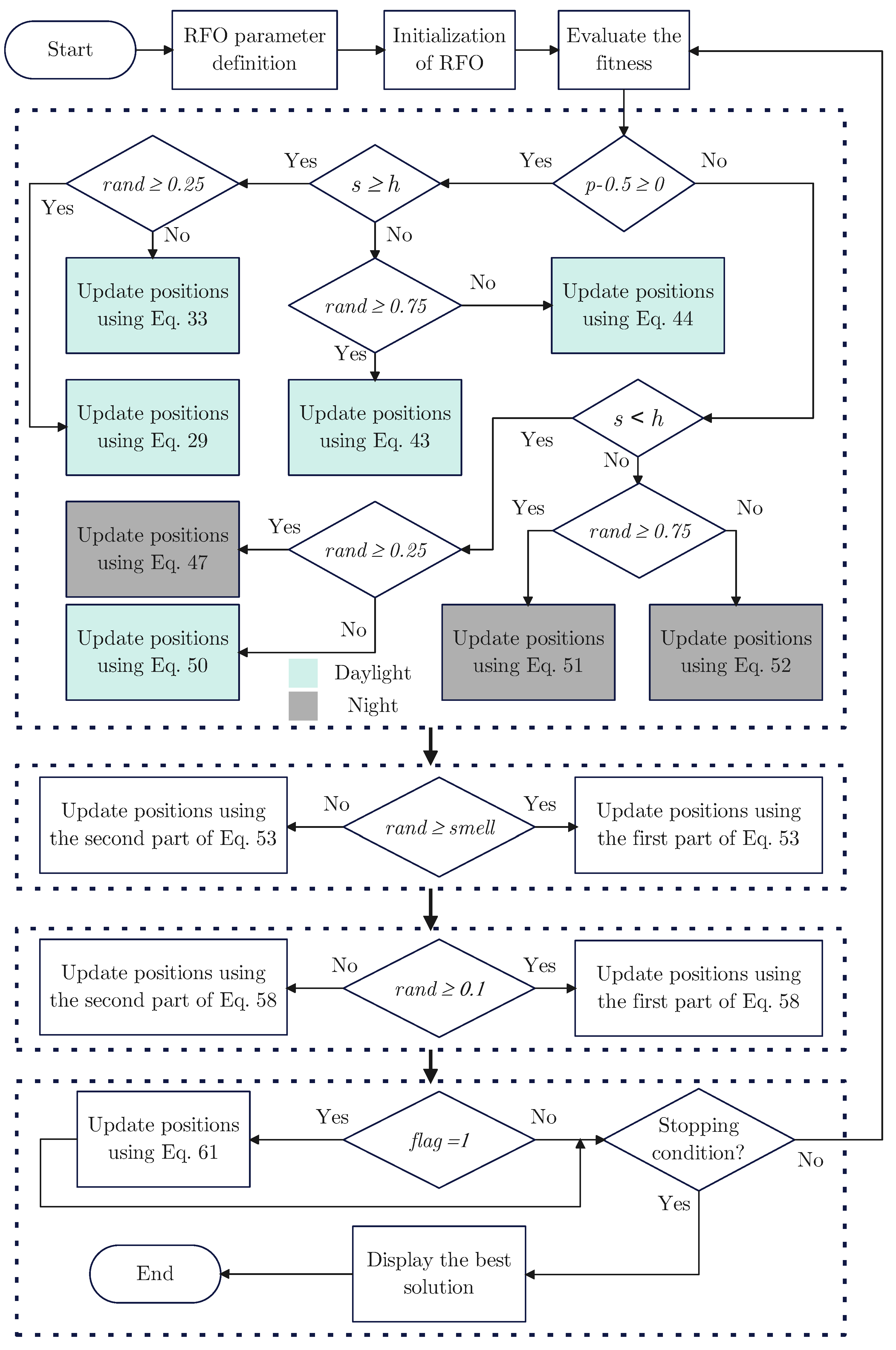
Overall, the flowchart in Figure 2 summarizes the key steps of Rüppell’s fox optimization algorithm based on the proposed mathematical model, and the pseudo-code is showing in Appendix A.

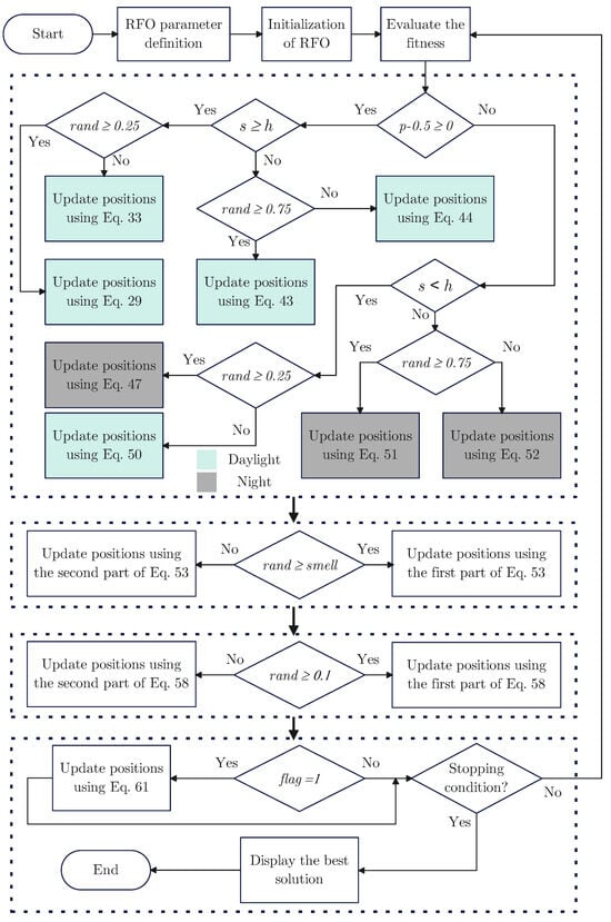
Figure 2. The flowchart of RFO.

4. Results and Discussion

In this section, the RFO algorithm is implemented to determine the optimal location and size of DG units alongside various metaheuristic methods, namely RIME, EFFO, WOA, GA, and SCA. The objective is to minimize total active power losses while maintaining bus voltages within acceptable limits and ensuring compliance with all system constraints. The algorithms are tested on the IEEE 33-bus and IEEE 69-bus radial distribution systems. System load flow is analyzed using the backward/forward sweep method, considering constant power loads under peak load conditions. The data for these test systems are provided in Appendix B. In this study, reducing power losses is prioritized over minimizing voltage deviation; therefore, the weighting factor ${\omega }_1=0.75$ is set higher than ${\omega }_2=0.25$ [52,53].

The optimization procedure involves selecting a specific number of DG units, identifying their optimal locations and sizes, and optimizing their power factor to reduce overall active power loss and improve the voltage profile by reducing voltage fluctuations. This method is shown by the numerous scenarios described in Table 1.

Table 1. The various operating PF of DG units across three distinct scenarios.

Scenario (Sc)	Power Factor (PF)	Decision Variables
01	Unity	Location(DGi), P(DGi)
02	0.95	Location(DGi), P(DGi)
03	Optimal	Location(DGi), P(DGi), and PF(DGi)

In the first scenario, tests were conducted using three DG units, each operating at a unity power factor. In this case, the DGs are considered PVDGs since they do not generate reactive power. In the second scenario, tests were performed with three DG units operating at a fixed power factor of $0.95$, classifying them as WTDGs. In the third case, the power factor is considered a decision variable, and its optimal value is established within the optimization problem. This approach yields a more optimum DG sizing than the initial two scenarios.

To ensure a fair comparison among the algorithms, the population size and the maximum number of iterations are uniformly set to 50 and 150, respectively, for all methods. All simulations in this study were performed using MATLAB R2021a on a personal computer equipped with an Intel Core i5-3230M CPU at 2.60 GHz and 8.00 GB of RAM. Each algorithm was executed 30 times in independent runs. In addition, Table 2 outlines the control parameters used for RFO and the five metaheuristic algorithms included in the performance evaluation simulation.

Table 2. The control parameters of the different metaheuristic algorithms.

Algorithms	Control Parameters
RFO	Constant for walk rate update $\beta =1\times {10}^{-10}$
RIME	Soft-rime control constant $W=5$
EEFO	-
WOA	Convergence parameter (a) linearly decreases from 2 to 0
GA	Distribution index for crossover and for mutation: 20
	Probability of crossover: $0.8$
	Probability of mutation: $0.2$
SCA	Parameter $a=2$

To assess the effectiveness of the proposed method, a comparison with the base case scenario was conducted prior to the installation of DG units. Table 3 summarizes the system data for each test case before the integration of DGs.

Table 3. Base case values of tested systems before DG installation.

Tested System	${\mathit{P}}_{\mathit{L}}$ (kW)	${\mathit{Q}}_{\mathit{L}}$ (kVAr)	TPL (kW)	TQL (kVAr)	${\mathit{V}}_{\mathit{max}}$ p.u (at Bus)	${\mathit{V}}_{\mathit{min}}$ p.u (at Bus)	${\mathit{V}}_{\mathit{d}}$ (%)
IEEE-33	3715	2300	202.6771	135.141	1 (1)	0.913 (18)	11.7094
IEEE-69	3801.89	2694.1	224.9606	102.147	1 (1)	0.909 (65)	9.9305

The simulation is carried out under the following assumptions:

• The distribution power network is modeled as a balanced radial system;
• The stochastic variability of solar irradiance and wind speed is neglected;
• The solar PV system is modeled as a constant active power (P) source, while the wind turbine is modeled as a constant PQ source;
• The solar PV system is assumed to operate with zero reactive power injection.

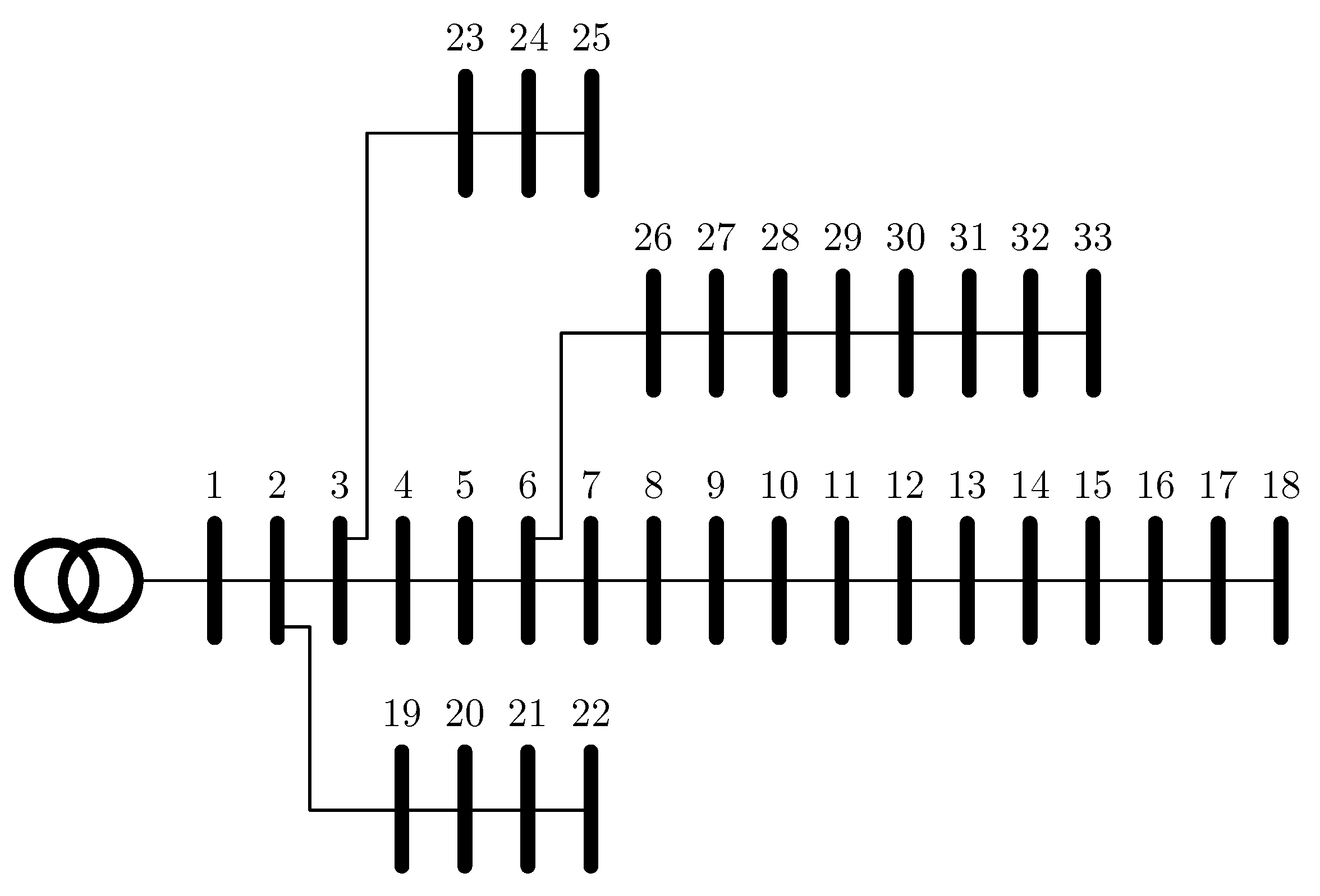
4.1. Case 01: IEEE 33-Bus Systems

In this section, three different scenarios are applied to the IEEE 33-bus system shown in Figure 3. The location, rated active power, and power factor of the units are decision variables that must be determined using six metaheuristic algorithms. The DGs can be installed on any bus from bus 2 to bus 33, and the rated active power of each DG unit can range from 0 MW to $2.0$ MW.

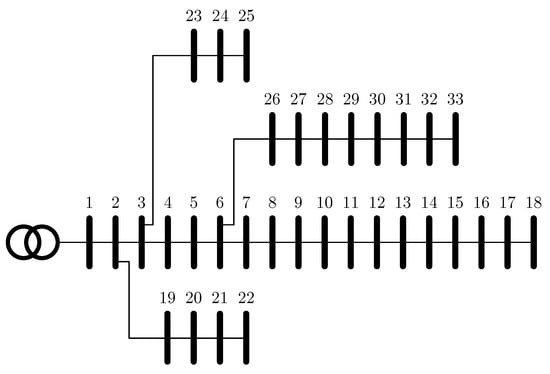
Figure 3. IEEE 33-bus distribution network.

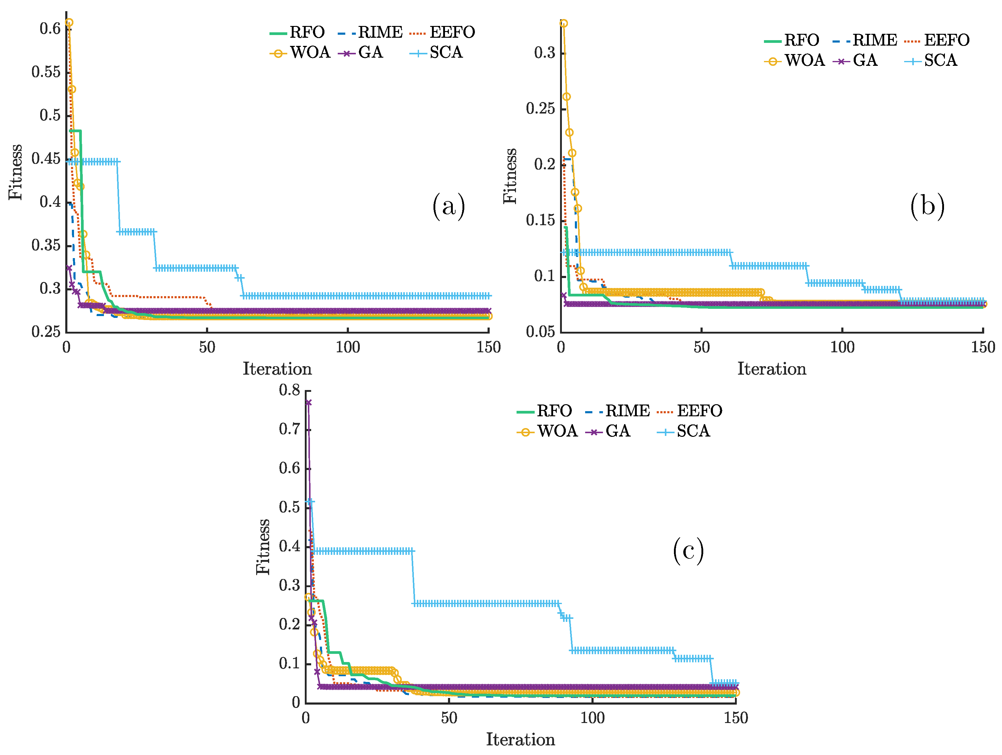
Figure 4 shows the convergence curves of six different applied algorithms under three scenarios.

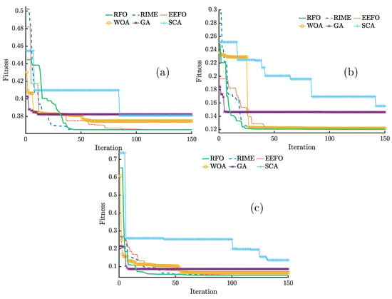
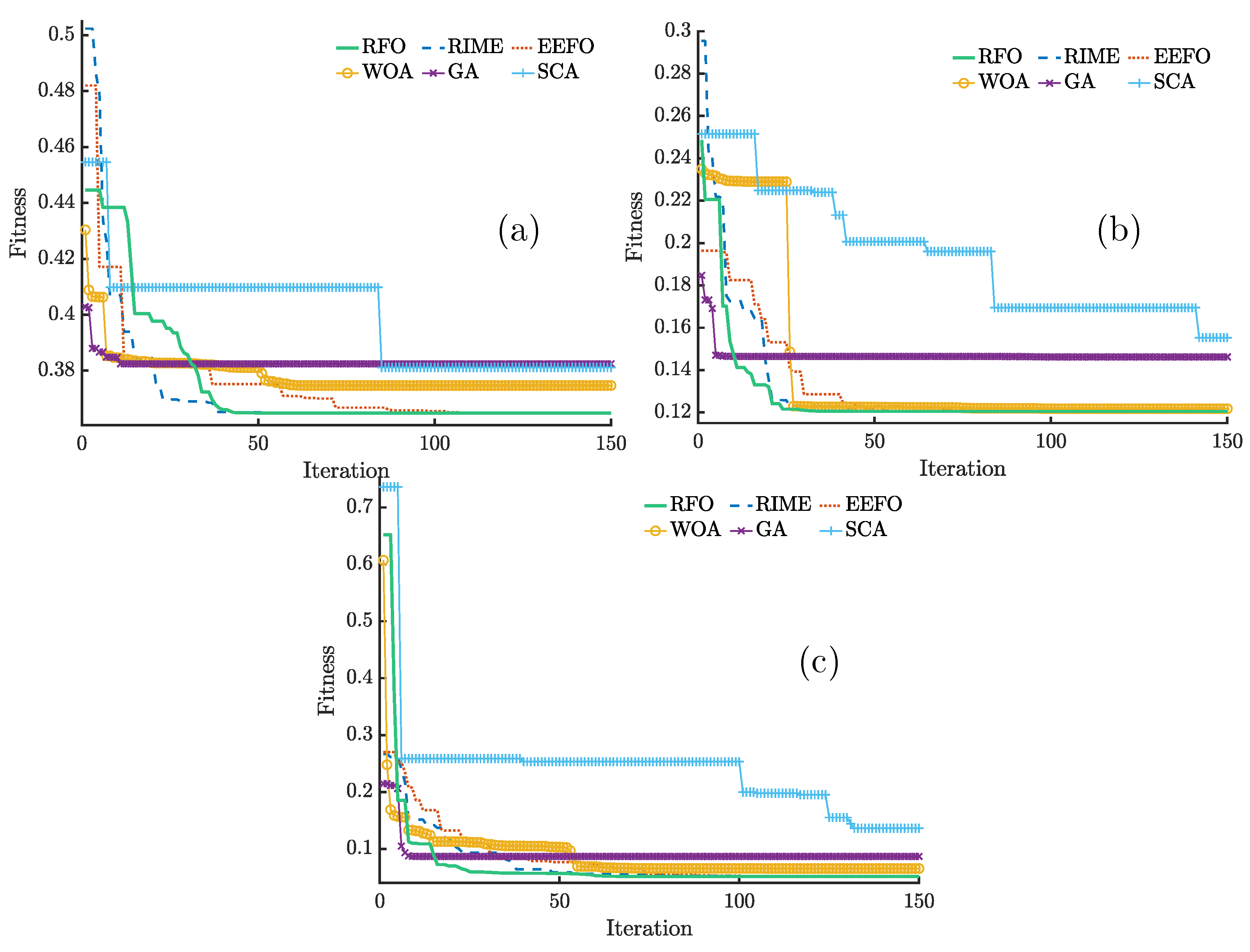
Figure 4. Convergence curves of different algorithms for (a) Scenario 1, (b) Scenario 2, and (c) Scenario 3 for the IEEE 33-bus systems.

In the first scenario (Figure 4a), the RFO algorithm exhibits the fastest and most stable convergence, achieving the lowest fitness value among all methods. RIME and EEFO also demonstrate competitive performance, although they converge slightly slower than RFO. WOA and GA settle at higher fitness values, while SCA exhibits the slowest convergence and the poorest performance.

In the second scenario (Figure 4b), a similar behavior is observed. RFO again outperforms other algorithms in terms of convergence speed. EEFO and RIME follow closely behind, showing quick descent within the first few iterations. GA and WOA maintain higher fitness values, and SCA reaches the highest fitness values.

In the third scenario (Figure 4c), the differences in algorithm performance become more remarkable. RFO rapidly converges to the lowest fitness value, demonstrating consistent robustness under varying conditions. Both EEFO and RIME perform relatively well, while WOA and GA show moderate improvement. SCA, however, exhibits a slow convergence rate and fails to reach a competitive solution.

Table 4 presents a statistical comparison (minimum, maximum, mean, and standard deviation of fitness values) of six different applied algorithms across three scenarios for the IEEE 33-bus system. The RFO algorithm consistently achieves the best overall performance, recording the lowest minimum fitness in all three scenarios, specifically $3.6482\times {10}^{-1}$, $1.2052\times {10}^{-1}$, and $5.1318\times {10}^{-2}$ for scenarios 1, 2, and 3, respectively. EEFO and RIME also demonstrate competitive performance with marginal differences from RFO, particularly in Scenario 2, where EEFO achieves the lowest mean of $1.2107\times {10}^{-1}$ and standard deviation of $1.2860\times {10}^{-3}$.

Table 4. Statistical comparison of six methods for the IEEE 33-bus systems.

	Sc	RFO	RIME	EEFO	WOA	GA	SCA
	1	$3.6482\times {10}^{-1}$	$3.6491\times {10}^{-1}$	$3.6483\times {10}^{-1}$	$3.7469\times {10}^{-1}$	$3.8245\times {10}^{-1}$	$3.8115\times {10}^{-1}$
Min	2	$1.2052\times {10}^{-1}$	$1.2052\times {10}^{-1}$	$1.2052\times {10}^{-1}$	$1.2180\times {10}^{-1}$	$1.4622\times {10}^{-1}$	$1.5537\times {10}^{-1}$
	3	$5.1318\times {10}^{-2}$	$5.1317\times {10}^{-2}$	$5.1316\times {10}^{-2}$	$6.5379\times {10}^{-2}$	$8.6605\times {10}^{-2}$	$1.3619\times {10}^{-1}$
	1	$3.9507\times {10}^{-1}$	$3.8474\times {10}^{-1}$	$3.7790\times {10}^{-1}$	$4.5546\times {10}^{-1}$	$4.9988\times {10}^{-1}$	$4.5145\times {10}^{-1}$
Max	2	$1.7325\times {10}^{-1}$	$1.6055\times {10}^{-1}$	$1.2485\times {10}^{-1}$	$2.2095\times {10}^{-1}$	$2.5974\times {10}^{-1}$	$2.1983\times {10}^{-1}$
	3	$2.7066\times {10}^{-1}$	$9.6383\times {10}^{-2}$	$6.1486\times {10}^{-2}$	$3.1782\times {10}^{-1}$	$6.8114\times {10}^{-1}$	$2.4359\times {10}^{-1}$
	1	$3.7962\times {10}^{-1}$	$3.7580\times {10}^{-1}$	$3.7097\times {10}^{-1}$	$4.1715\times {10}^{-1}$	$4.2701\times {10}^{-1}$	$4.1632\times {10}^{-1}$
Mean	2	$1.4393\times {10}^{-1}$	$1.2728\times {10}^{-1}$	$1.2107\times {10}^{-1}$	$1.6956\times {10}^{-1}$	$1.9073\times {10}^{-1}$	$1.8098\times {10}^{-1}$
	3	$1.1390\times {10}^{-1}$	$6.8626\times {10}^{-2}$	$5.4106\times {10}^{-2}$	$1.4164\times {10}^{-1}$	$2.5840\times {10}^{-1}$	$1.8429\times {10}^{-1}$
	1	$7.6835\times {10}^{-3}$	$6.4594\times {10}^{-3}$	$5.4691\times {10}^{-3}$	$2.2204\times {10}^{-2}$	$2.7997\times {10}^{-2}$	$2.1442\times {10}^{-2}$
std	2	$1.6969\times {10}^{-2}$	$1.3016\times {10}^{-2}$	$1.2860\times {10}^{-3}$	$2.7253\times {10}^{-2}$	$2.3873\times {10}^{-2}$	$2.1169\times {10}^{-2}$
	3	$5.4604\times {10}^{-2}$	$1.8467\times {10}^{-2}$	$3.0454\times {10}^{-3}$	$5.4036\times {10}^{-2}$	$1.2107\times {10}^{-1}$	$2.9579\times {10}^{-2}$

In contrast, several algorithms, such as GA and SCA, demonstrate significantly higher mean and standard deviation values, signifying considerable solution instability. Conversely, WOA demonstrates modest performance, surpassing GA and SCA, although it remains inferior to the leading approaches.

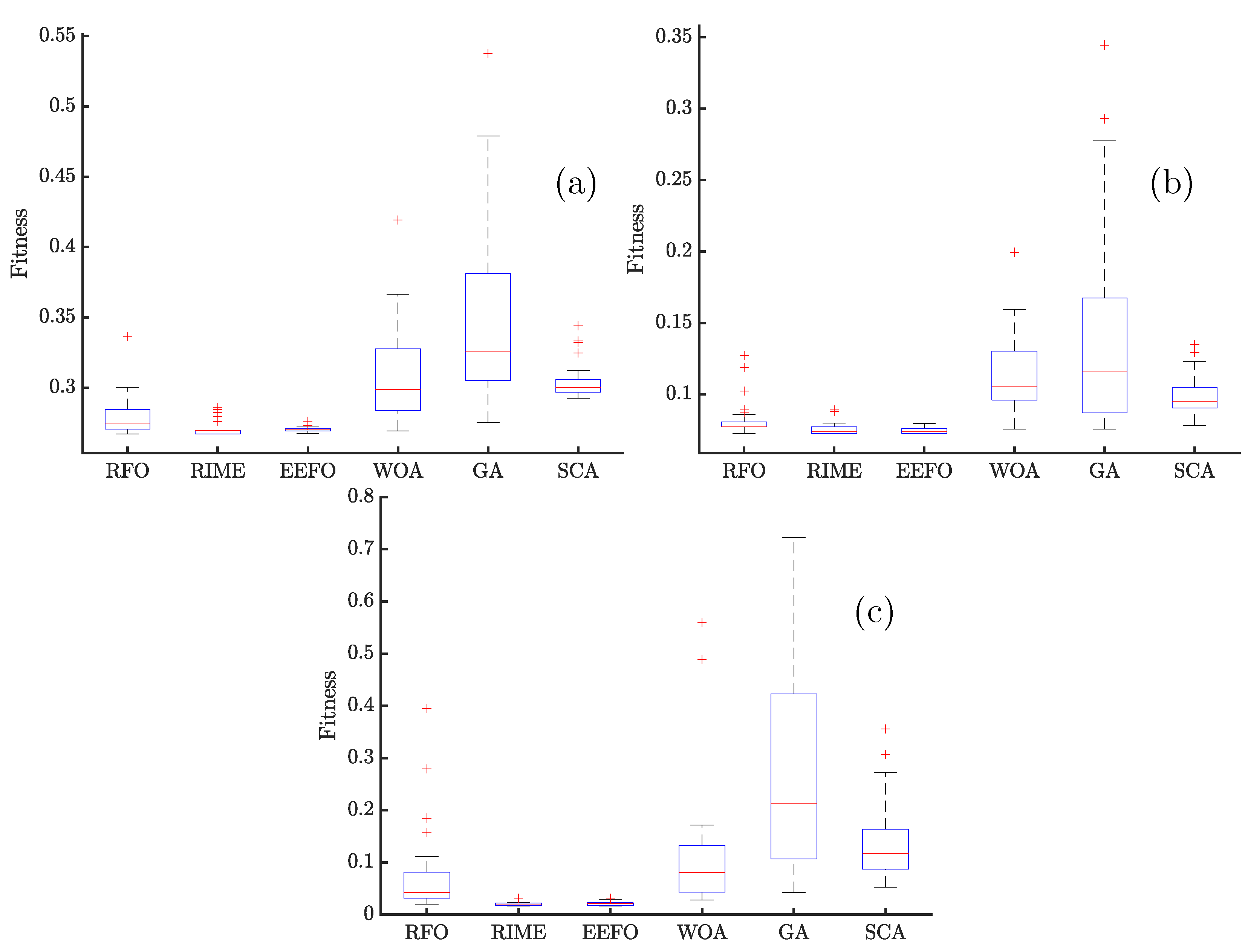
Figure 5 illustrates the box plots of fitness values obtained by different optimization algorithms across three scenarios for the IEEE 33-bus system.

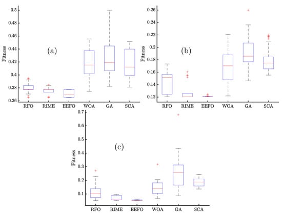
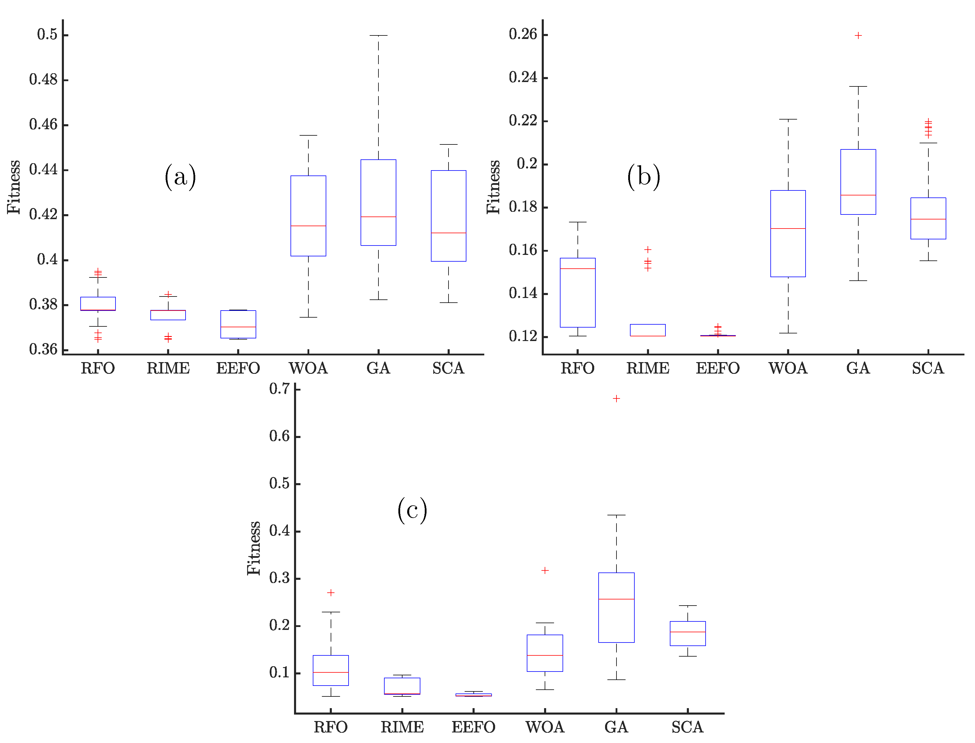
Figure 5. Box plot of different algorithms for (a) Scenario 1, (b) Scenario 2, and (c) Scenario 3 for the IEEE 33-bus systems.

For Scenario 1 (Figure 5a), RFO, RIME, and EEFO display tight distributions with minimal variance, indicating high reliability and stable convergence. Notably, EEFO has the lowest spread, consistently converging near its optimal value. In contrast, WOA, GA, and SCA show broader interquartile ranges (IQRs) and several outliers, reflecting instability and less reliable optimization performance.

In Scenario 2 (Figure 5b), EEFO demonstrates superior robustness with a narrow IQR and a very low median fitness. RIME also shows consistent performance, while RFO exhibits a slightly wider distribution but still maintains competitive results. WOA, GA, and SCA again exhibit larger spreads and higher medians, confirming their weaker optimization capabilities and higher variability in this scenario.

Scenario 3 (Figure 5c) further highlights the superiority of EEFO and RIME, both attaining concentrated distributions with minimal median fitness values. RFO shows remarkable performance but with slightly broader variance. In contrast, GA and WOA demonstrate the most significant variance and occurrence of outliers, signifying considerable inconsistency in attaining optimal solutions. SCA persists in demonstrating weak and inconsistent performance.

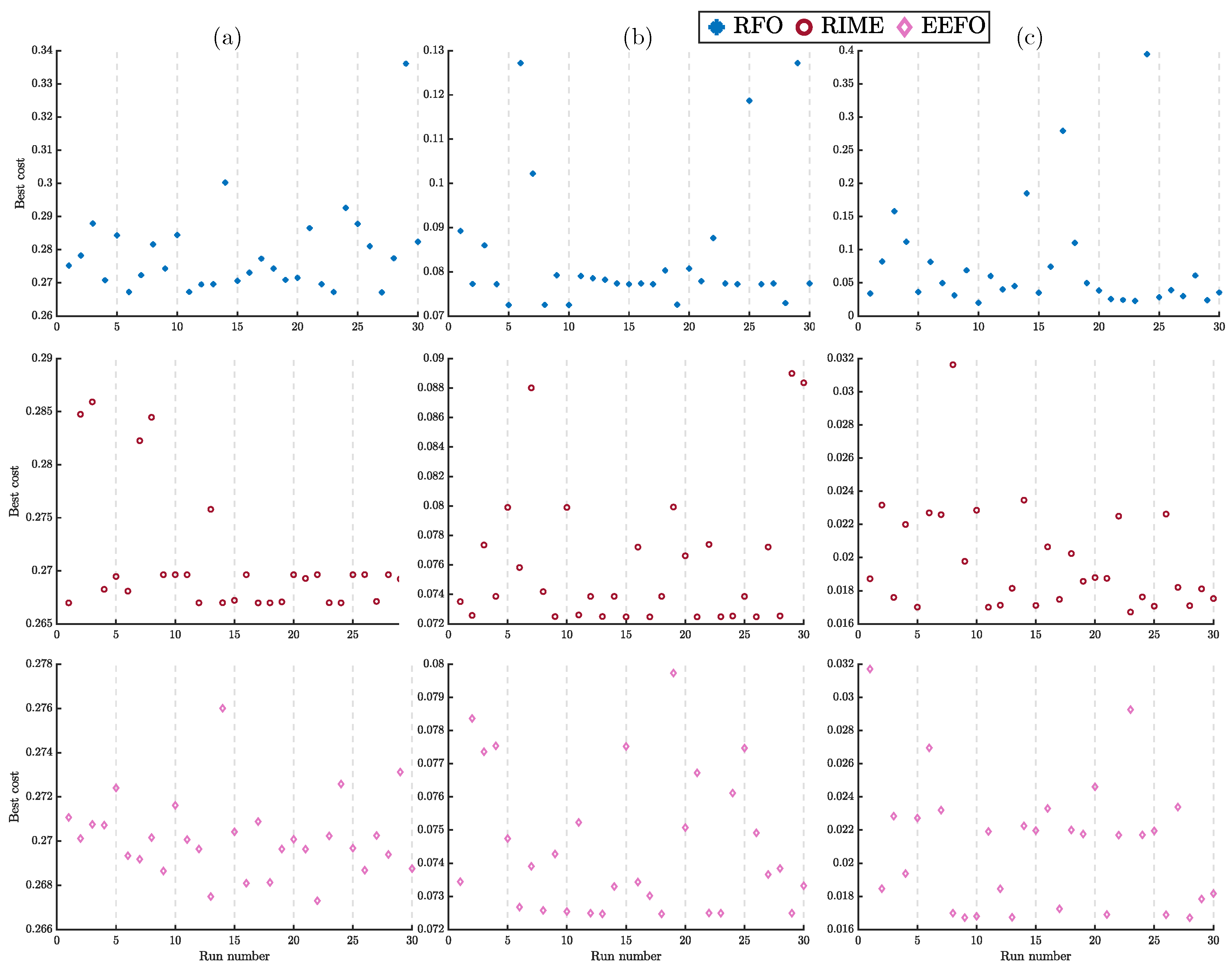
RFO offers the most robust and efficient convergence characteristics, followed closely by EEFO and RIME, while WOA, GA, and SCA demonstrate relatively inferior optimization capabilities in the tested scenarios. For that, only the best objective function values obtained from each run of the RFO, RIME, and EEFO are shown in Figure 6.

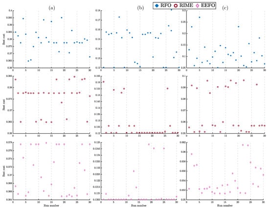
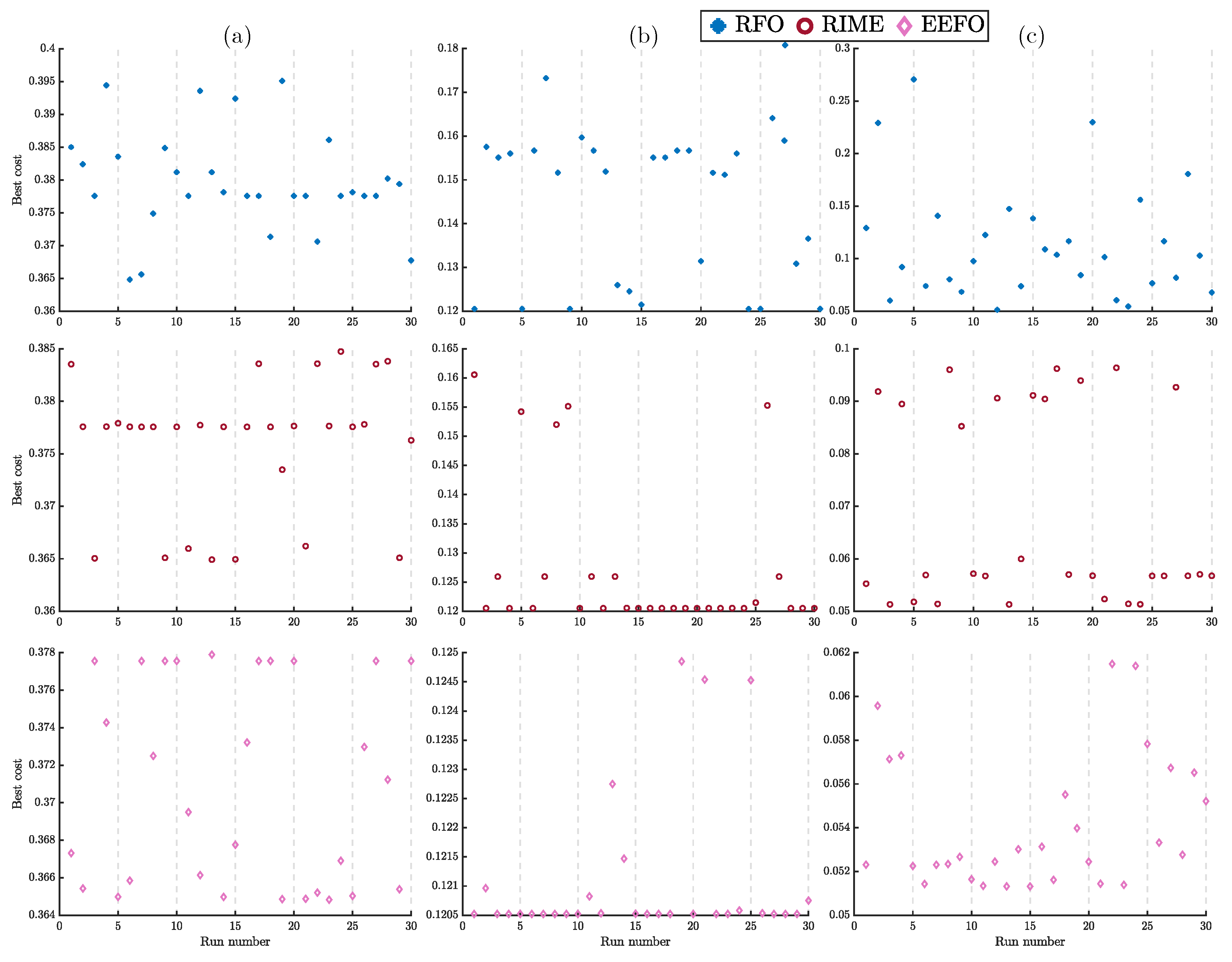
Figure 6. Objective function values obtained from each run of the RFO, RIME, and EEFO for (a) Scenario 1, (b) Scenario 2, and (c) Scenario 3 for the IEEE 33-bus systems.

For the first scenario, the results of RFO show moderate variability. On the other hand, RIME and EEFO show better consistency, particularly EEFO. This consistency gap between the algorithms becomes more pronounced in the second scenario, especially for EEFO, where it produces nearly identical objective values in most runs. RIME closely follows EEFO, exhibiting limited variance and a clear tendency to converge to optimal or near-optimal solutions. RFO, while still competent, demonstrates more scattered results.

The final scenario further highlights the robustness of EEFO, with its results tightly clustered around the lowest achieved objective value. RIME also performs well, though with occasional deviations, while RFO shows the widest spread, including several runs that yield comparatively higher objective values.

The optimal solutions, including the location, size, and power factor of each DG unit obtained by the six applied optimization methods, are summarized in Table 5. The DG locations identified by RFO, RIME, and EEFO are generally consistent across all three scenarios. In contrast, the locations selected by WOA, GA, and SCA vary significantly between scenarios.

Table 5. The best location and sizes of DGs in (kW/kVAr) obtained for the IEEE 33-bus systems.

		Scenario 01		Scenario 02			Scenario 03
Algo	DG	Loc	${\mathit{P}}_{\mathit{DG}}$	Loc	${\mathit{P}}_{\mathit{DG}}$	${\mathit{Q}}_{\mathit{DG}}$	Loc	${\mathit{P}}_{\mathit{DG}}$	${\mathit{Q}}_{\mathit{DG}}$	${\mathit{PF}}_{\mathit{DG}}$
RFO	1	13	$1125.784$	24	$1179.043$	$387.5328$	13	$825.9447$	$400.2203$	$0.8999158$
	2	24	$1065.244$	30	$1411.843$	$464.0503$	30	$1087.705$	$1035.279$	$0.7243477$
	3	30	$1523.972$	13	$909.0967$	$298.8056$	24	$1121.78$	$539.4451$	$0.9012124$
RIME	1	24	$1054.137$	30	$1411.838$	$464.0487$	24	$1111.956$	$528.3639$	$0.9032193$
	2	13	$1120.421$	24	$1178.825$	$387.4609$	13	$829.7859$	$397.4739$	$0.9018719$
	3	30	$1538.002$	13	$909.2089$	$298.8425$	30	$1082.122$	$1043.182$	$0.7199416$
EEFO	1	13	$1129.136$	30	$1411.843$	$464.0503$	30	$1083.690$	$1036.145$	$0.7227844$
	2	30	$1522.839$	24	$1179.043$	$387.5327$	13	$827.5979$	$402.7751$	$0.8991668$
	3	24	$1063.010$	13	$909.0967$	$298.8056$	24	$1109.037$	$548.6703$	$0.8963098$
WOA	1	30	$1680.392$	24	$1235.987$	$406.2493$	30	$1109.023$	$841.8242$	$0.7965195$
	2	24	$1039.312$	14	$869.7179$	$285.8625$	14	$697.8561$	$590.7923$	$0.7632252$
	3	15	$945.4812$	30	$1405.729$	$462.0407$	24	$1172.795$	$617.6266$	$0.8848044$
GA	1	15	$712.3350$	24	$636.3638$	$209.1627$	24	$833.9301$	$648.0065$	$0.7896301$
	2	31	$1069.080$	30	$1460.99$	$480.2041$	14	$641.8102$	$239.9634$	$0.936672$
	3	06	$1610.605$	11	$1118.536$	$367.6449$	29	$1410.462$	$1321.97$	$0.7296245$
SCA	1	25	$735.0925$	30	$1572.341$	$516.8036$	8	$261.8669$	$505.5602$	$0.4599358$
	2	13	$1186.920$	24	$776.9385$	$255.3673$	13	$907.7172$	0	1
	3	29	$1529.391$	10	$983.0985$	$323.1288$	29	$1182.764$	$1172.215$	$0.7102669$

Similarly, the DG sizes determined by RFO, RIME, and EEFO exhibit only minor variations across scenarios. On the other hand, consistent with the variation in DG placement, the sizes obtained by WOA, GA, and SCA differ noticeably from one scenario to another for each algorithm.

Regarding the power factor in Scenario 3, RFO, RIME, and EEFO yield closely matching results. Notably, all three methods identify Bus 30 as one of the optimal locations for a DG unit, with corresponding power ratings of $1087.705$ kW (RFO), $1082.122$ kW (RIME), and $1083.690$ kW (EEFO). In comparison, WOA also selects Bus 30 but assigns a slightly higher DG rating of $1109.023$ kW with a distinct power factor of $0.7965195$.

The total installed DG power summarized in Table 6 reveals that RFO, RIME, and EEFO consistently yield higher and closely matching total active and reactive power outputs across all three scenarios, while WOA, GA, and especially SCA result in lower total active power, most notably in Scenario 3; highlighting a significant variation in DG sizing performance among the algorithms.

Table 6. The total installed power of DGs in (kW/kVAr) obtained for the IEEE 33-bus systems.

	Scenario 01	Scenario 02		Scenario 03
Algo	${\mathit{P}}_{{\mathit{DG}}_{\mathit{tot}}}$	${\mathit{P}}_{{\mathit{DG}}_{\mathit{tot}}}$	${\mathit{Q}}_{{\mathit{DG}}_{\mathit{tot}}}$	${\mathit{P}}_{{\mathit{DG}}_{\mathit{tot}}}$	${\mathit{Q}}_{{\mathit{DG}}_{\mathit{tot}}}$
RFO	$3715.00$	$3499.983$	$1150.389$	$3035.430$	$1974.944$
RIME	$3712.560$	$3499.871$	$1150.352$	$3023.864$	$1969.02$
EEFO	$3714.986$	$3499.983$	$1150.389$	$3020.325$	$1987.590$
WOA	$3665.185$	$3511.434$	$1154.152$	$2979.674$	$2050.243$
GA	$3392.020$	$3215.889$	$1057.012$	$2886.203$	$2209.94$
SCA	$3451.403$	$3332.378$	$1095.3$	$2352.348$	$1677.776$

Table 7 presents the total active and reactive power losses after DG installation in the IEEE 33-bus system, along with the corresponding percentage reductions for each scenario, clearly demonstrating that RFO, RIME, and EEFO consistently outperform the other algorithms in minimizing losses, with the highest overall loss reductions observed across all methods in scenario 3.

Table 7. The power losses after DGs installation for the IEEE 33-bus systems.

	Sc	RFO	RIME	EEFO	WOA	GA	SCA
	1	$87.538$	$87.7924$	$87.6246$	$89.2076$	$91.5604$	$88.1741$
TPL(kW)	2	$30.3419$	$30.3427$	$30.3419$	$30.1865$	$35.4284$	$35.325$
	3	$12.0712$	$12.0516$	$12.0614$	$14.6928$	$18.684$	$30.7716$
	1	$60.737$	$60.936$	$60.7929$	$62.9088$	$64.5453$	$61.4224$
QPL(kVAr)	2	$22.5974$	$22.5977$	$22.5974$	$22.6843$	$25.6925$	$25.8553$
	3	$10.0559$	$10.0275$	$10.0369$	$12.1826$	$15.1082$	$22.1714$
	1	$56.8091$	$56.6836$	$56.7664$	$55.9853$	$54.8245$	$56.4953$
$P_{red}$ (%)	2	$85.0294$	$85.0291$	$85.0294$	$85.1061$	$82.5198$	$82.5708$
	3	$94.0441$	$94.0538$	$94.0489$	$92.7507$	$90.7814$	$84.8174$
	1	$55.0566$	$54.9093$	$55.0152$	$53.4495$	$52.2386$	$54.5494$
$Q_{red}$ (%)	2	$83.2786$	$83.2784$	$83.2786$	$83.2144$	$80.9884$	$80.8679$
	3	$92.559$	$92.58$	$92.573$	$90.9852$	$88.8204$	$83.5939$

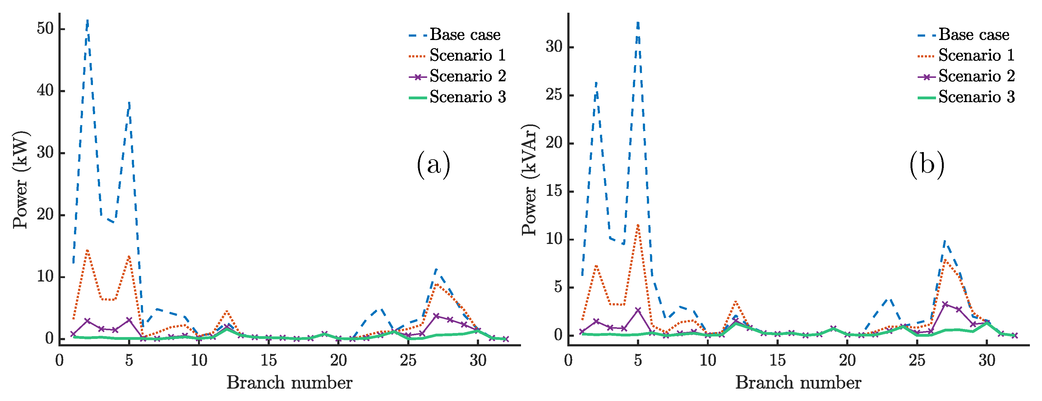
Figure 7 illustrates the branch active and reactive power losses in the IEEE 33-bus system, both with and without DGs, under different scenarios using the RFO algorithm, where the third scenario yields the minimum losses.

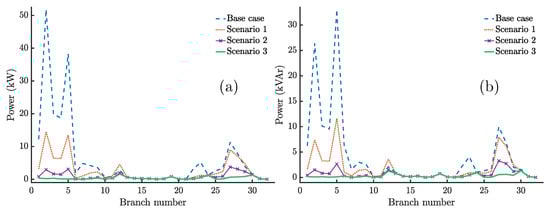
Figure 7. Branch (a) active and (b) reactive power losses for the IEEE 33-bus system under different scenarios using RFO.

Table 8 presents the maximum and minimum bus voltages, along with their corresponding bus numbers, for the IEEE 33-bus system under three different scenarios as obtained by the six applied methods. The results indicate that the minimum voltage improves across scenarios, with the third scenario consistently achieving the best voltage profile. The voltage deviation $V_d$ is lowest in Scenario 3 for all methods, with RFO, RIME, and EEFO exhibiting the most stable and tightly regulated voltage profiles compared to the others.

Table 8. The obtained voltages in pu after DGs installation for the IEEE 33-bus systems.

	Sc	RFO	RIME	EEFO	WOA	GA	SCA
	1	$0.9876452$ (33)	$0.9879646$ (33)	$0.9876455$ (33)	$0.9883353$ (8)	$0.9824855$ (25)	$0.9825155$ (33)
$V_{min}$ (at bus)	2	$0.9940811$ (22)	$0.9940810$ (22)	$0.9940811$ (22)	$0.99354$ (8)	$0.9908983$ (24)	$0.9863899$ (18)
	3	$0.9940696$ (22)	$0.9940612$ (22)	$0.9940646$ (22)	$0.9940574$ (22)	$0.9931436$ (18)	$0.9820739$ (25)
	1	1 (1)	1 (1)	1 (1)	1 (1)	1 (1)	$1.001104$ (13)
$V_{max}$ (at bus)	2	$1.003898$ (13)	$1.003903$ (13)	$1.003898$ (13)	$1.004014$ (14)	$1.005002$ (11)	$1.006579$ (30)
	3	$1.004331$ (13)	$1.004352$ (13)	$1.004408$ (13)	$1.006377$ (14)	$1.011766$ (29)	$1.007498$ (29)
	1	$0.16356$	$0.16017$	$0.1623$	$0.1783$	$0.17452$	$0.21945$
$V_d$(%)	2	$0.032969$	$0.032958$	$0.032969$	$0.040383$	$0.060483$	$0.098599$
	3	$0.026595$	$0.026882$	$0.026733$	$0.044036$	$0.069862$	$0.089281$

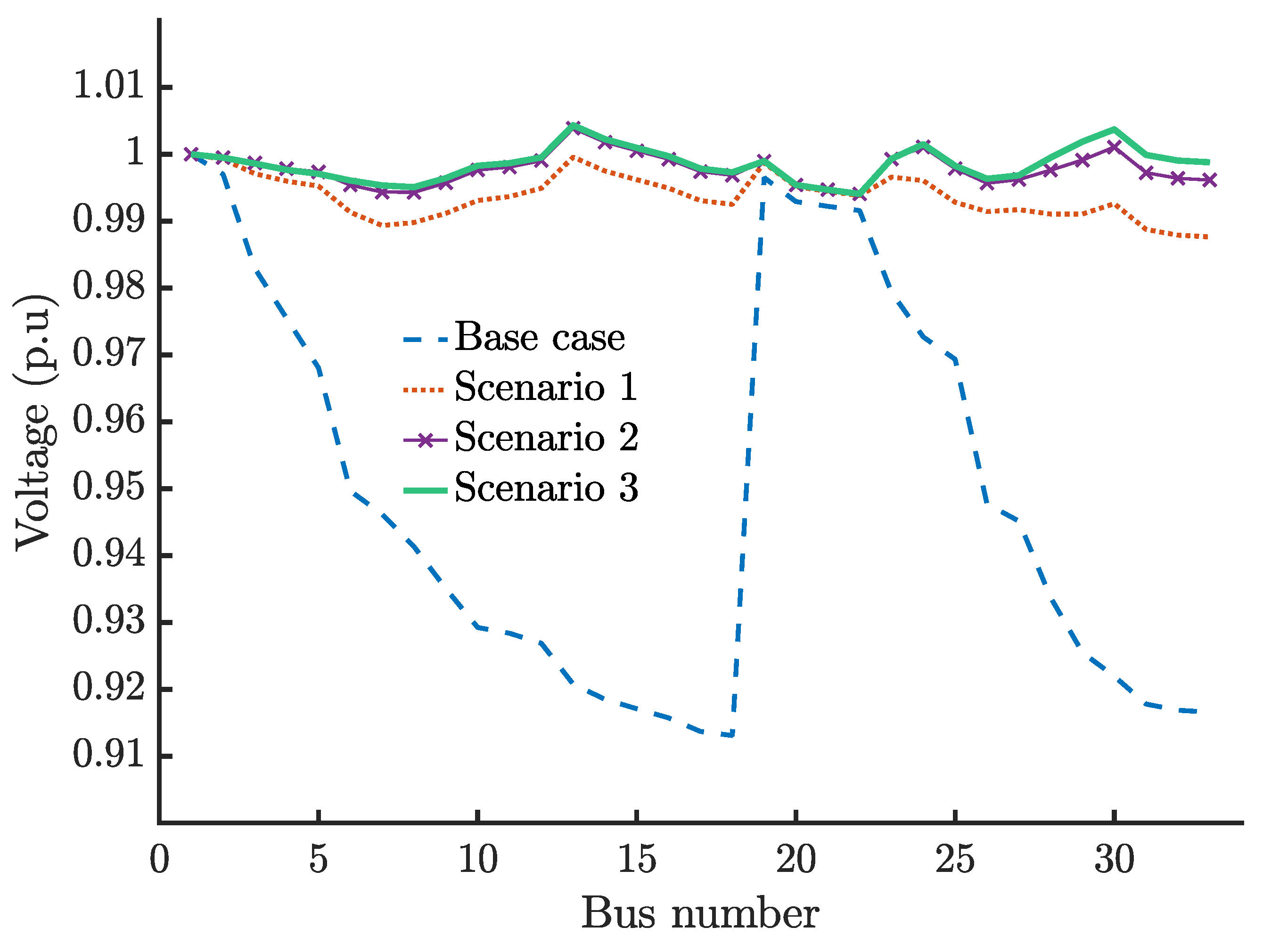
Figure 8 illustrates the voltage profiles of all buses in the IEEE 33-bus system for the base case without DG units and for the three scenarios optimized using the RFO algorithm. In the base case, all bus voltages are lower compared to the DG-integrated scenarios, demonstrating a clear improvement in the voltage profile after DG installation. Notably, several buses in the base case exhibit voltages below $0.92$ pu, which are significantly improved and brought within the acceptable range of $[0.95,1.05]$ pu in all DG scenarios. Among the four curves, the best voltage profile is that of the third scenario.

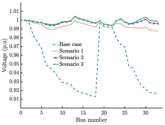
Figure 8. Bus voltage for the IEEE 33-bus system under different scenarios using RFO.

4.2. Case 02: IEEE 69-Bus Systems

In this section, similar to the IEEE 33-bus system, the six previously applied algorithms are implemented on the IEEE 69-bus system, as illustrated in Figure 9, to determine the optimal location, size, and power factor of DG. The candidate locations range from bus 2 to bus 69, and the rated size of each DG varies from 0 MW to 2 MW.

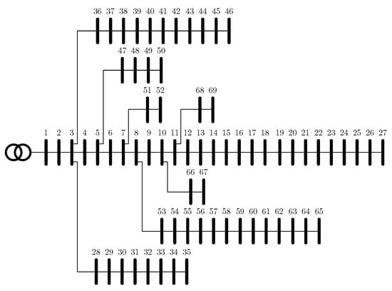
Figure 9. IEEE 69-bus distribution network.

Figure 10 presents the convergence curves of RFO, RIME, EEFO, WOA, GA, and SCA algorithms in the IEEE 69-bus system for scenarios 1, 2, and 3.

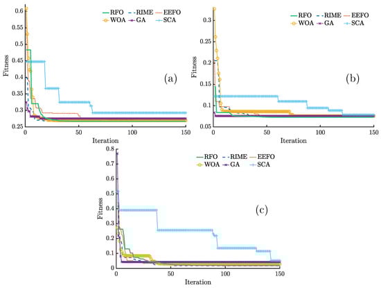
Figure 10. Convergence curves of different algorithms for (a) Scenario 1, (b) Scenario 2, and (c) Scenario 3 for the IEEE 69-bus system.

In the first scenario, all algorithms demonstrate rapid initial convergence. RIME achieves the lowest fitness value in the shortest time, closely followed by RFO. EEFO also converges effectively but requires more iterations to stabilize. WOA and GA show relatively good convergence, though with slightly higher final fitness values. Notably, SCA converges slowly and stagnates at a significantly higher fitness level.

In the second scenario, RFO outperforms other algorithms in both convergence speed and solution quality, followed by RIME and GA. However, GA shows rapid convergence but with higher final fitness values than the three top-performing algorithms: RFO, RIME, and EEFO. WOA also lags in this scenario, while SCA continues to show the slowest and least accurate convergence.

In the third scenario, the complexity of the optimization task increases with the inclusion of the power factor as a decision variable. Despite this, RFO, RIME, and EEFO maintain superior convergence behavior, achieving lower fitness values with fewer iterations. However, RFO requires more iterations to stabilize. GA and WOA initially perform well but eventually converge to local optima, resulting in higher final fitness values. SCA again shows poor convergence performance, with high final fitness values and minimal improvement across all iterations.

The statistical comparison of several methods applied to the IEEE 69-bus system across three scenarios is presented in Table 9. RFO shows moderate efficacy across all scenarios. In Scenario 1, it attains an acceptable mean of $2.7896\times {10}^{-1}$ and exhibits reasonable stability, although less consistent than EEFO and RIME. Scenario 2 demonstrates similar characteristics, presenting a competitive minimum of $7.2481\times {10}^{-2}$ and a higher standard deviation, indicating greater variability. In Scenario 3, a minimum of $1.9924\times {10}^{-2}$, along with RFO’s high mean and significant standard deviation of $8.2575\times {10}^{-2}$, suggests possible convergence issues and occasional unsatisfactory results.

Table 9. Statistical comparison of six methods for the IEEE 69-bus systems.

	Sc	RFO	RIME	EEFO	WOA	GA	SCA
	1	$2.6712\times {10}^{-1}$	$2.6698\times {10}^{-1}$	$2.6730\times {10}^{-1}$	$2.6917\times {10}^{-1}$	$2.7524\times {10}^{-1}$	$2.9259\times {10}^{-1}$
Min	2	$7.2481\times {10}^{-2}$	$7.2474\times {10}^{-2}$	$7.2471\times {10}^{-2}$	$7.5700\times {10}^{-2}$	$7.5621\times {10}^{-2}$	$7.8410\times {10}^{-2}$
	3	$1.9924\times {10}^{-2}$	$1.6712\times {10}^{-2}$	$1.6712\times {10}^{-2}$	$2.7976\times {10}^{-2}$	$4.2201\times {10}^{-2}$	$5.2529\times {10}^{-2}$
	1	$3.3609\times {10}^{-1}$	$2.8592\times {10}^{-1}$	$2.7600\times {10}^{-1}$	$4.1912\times {10}^{-1}$	$5.3767\times {10}^{-1}$	$3.4401\times {10}^{-1}$
Max	2	$1.2720\times {10}^{-1}$	$8.8987\times {10}^{-2}$	$7.9732\times {10}^{-2}$	$1.9949\times {10}^{-1}$	$3.4456\times {10}^{-1}$	$1.3505\times {10}^{-1}$
	3	$3.9466\times {10}^{-1}$	$3.1631\times {10}^{-2}$	$3.1712\times {10}^{-2}$	$5.5896\times {10}^{-1}$	$1.0001\times {10}^{+4}$	$3.5575\times {10}^{-1}$
	1	$2.7896\times {10}^{-1}$	$2.7113\times {10}^{-1}$	$2.7014\times {10}^{-1}$	$3.1049\times {10}^{-1}$	$3.5091\times {10}^{-1}$	$3.0545\times {10}^{-1}$
Mean	2	$8.3505\times {10}^{-2}$	$7.6046\times {10}^{-2}$	$7.4523\times {10}^{-2}$	$1.1461\times {10}^{-1}$	$1.4319\times {10}^{-1}$	$9.9527\times {10}^{-2}$
	3	$7.5865\times {10}^{-2}$	$1.9761\times {10}^{-2}$	$2.1018\times {10}^{-2}$	$1.1226\times {10}^{-1}$	$1.0003\times {10}^{+3}$	$1.3786\times {10}^{-1}$
	1	$1.3662\times {10}^{-2}$	$5.9018\times {10}^{-3}$	$1.7759\times {10}^{-3}$	$3.4906\times {10}^{-2}$	$6.3091\times {10}^{-2}$	$1.3694\times {10}^{-2}$
std	2	$1.5111\times {10}^{-2}$	$4.8580\times {10}^{-3}$	$2.1197\times {10}^{-3}$	$2.6109\times {10}^{-2}$	$7.0510\times {10}^{-2}$	$1.3428\times {10}^{-2}$
	3	$8.2575\times {10}^{-2}$	$3.2080\times {10}^{-3}$	$3.8521\times {10}^{-3}$	$1.2071\times {10}^{-1}$	$3.0514\times {10}^{+3}$	$7.1971\times {10}^{-2}$

EEFO regularly surpasses all other algorithms in the examined cases, exhibiting both accuracy and dependability. In Scenario 1, it attains a minimal mean fitness of $2.7014\times {10}^{-1}$ and a standard deviation of $1.7759\times {10}^{-3}$, demonstrating strong performance and reliability. In Scenario 2, EEFO achieves the optimal minimum of $7.2471\times {10}^{-2}$, the lowest mean of $7.4523\times {10}^{-2}$, and the smallest standard deviation of $2.1197\times {10}^{-3}$, surpassing all competitors. Scenario 3 further validates EEFO’s robustness, exhibiting one of the lowest minimums of $1.6712\times {10}^{-2}$, a low mean of $2.1018\times {10}^{-2}$, and a minimal standard deviation of $3.8521\times {10}^{-3}$.

Among the other algorithms, RIME also demonstrates strong and consistent performance, particularly excelling in Scenario 3, with the best minimum and mean fitness values, as well as low standard deviations across the board. In contrast, GA and SCA perform poorly and unreliably; SCA consistently records higher means and variances. WOA falls in the mid-range and tends to show higher variability, especially in scenarios 1 and 3.

Figure 11 illustrates the box plots for several applied algorithms in scenarios 1–3 of the IEEE 69-bus system. According to the box plots, in Scenario 1, RFO demonstrates a closely centered median and a minimal box height, signifying low variability and reliable performance, surpassing WOA, GA, and SCA in consistency. In Scenario 2, RFO demonstrates a stable and consistent performance, with fewer deviations and a slightly better median when compared to GA and WOA. Its distribution remains compact, indicating reliability under moderate conditions. However, in Scenario 3, RFO’s performance becomes less stable; its interquartile range increases, the median rises above those of RIME and EEFO, and moderate outliers emerge.

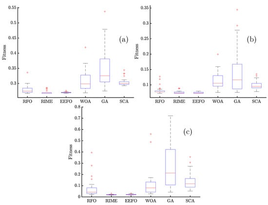
Figure 11. Box plot of different algorithms for (a) Scenario 1, (b) Scenario 2, and (c) Scenario 3 for the IEEE 69-bus systems (the y-axis in Scenario 3 was limited to improve visibility due to an extremely high maximum value in the GA results).

These changes suggest that RFO may struggle with adaptability in more complex situations. Although RFO outperforms GA and SCA in this context, it is surpassed by RIME and EEFO in terms of both consistency and central tendency.

The best fitness values for each run of the RFO, RIME, and EEFO algorithms are illustrated in Figure 12 for the three scenarios. Both RFO and RIME demonstrate stability across all scenarios, with RFO showing remarkably consistent results in Scenario 2. In contrast, EEFO exhibits greater variability in the obtained solutions compared to its performance in the IEEE 33-bus system.

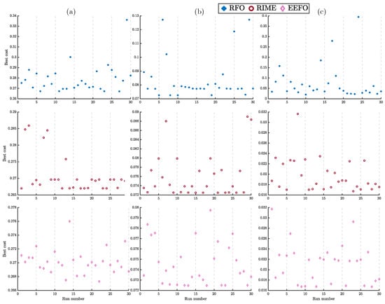
Figure 12. Objective function values obtained from each run of the RFO, RIME, and EEFO for (a) Scenario 1, (b) Scenario 2, and (c) Scenario 3 for the IEEE 69-bus systems.

The best locations and sizes of DGs obtained for the IEEE 69-bus system using six different algorithms across the three scenarios are presented in Table 10. Bus 61 is consistently identified as an optimal location in all scenarios, except in Scenario 3 for the SCA algorithm. In the RFO, RIME, and EEFO algorithms, buses 61 and 11 are frequently selected, except in Scenario 3 for the RFO method. The alternative DG position fluctuates among cases for these three methods, indicating a degree of flexibility in the placement technique. Moreover, the optimal sizes for a given location generally remain stable across each scenario. In contrast, the WOA, GA, and SCA algorithms yield different optimal locations and sizes for each scenario, suggesting less consistency in their solution patterns.

Table 10. The best location and sizes of DGs in (kW/kVAr) obtained for the IEEE 69-bus systems.

		Scenario 01		Scenario 02			Scenario 03
Algo	DG	Loc	${\mathit{P}}_{\mathit{DG}}$	Loc	${\mathit{P}}_{\mathit{DG}}$	${\mathit{Q}}_{\mathit{DG}}$	Loc	${\mathit{P}}_{\mathit{DG}}$	${\mathit{Q}}_{\mathit{DG}}$	${\mathit{PF}}_{\mathit{DG}}$
RFO	1	11	$778.0838$	61	$1925.72$	$632.9536$	61	$1709.631$	$1152.700$	$0.829141$
	2	17	$491.9404$	20	$402.9199$	$132.4334$	23	$318.0294$	$252.7801$	$0.7828382$
	3	61	$1999.216$	11	$644.5698$	$211.8598$	10	$647.0536$	$566.5961$	$0.7523322$
RIME	1	11	$820.2928$	61	$1925.039$	$632.7298$	11	$534.9744$	$387.7978$	$0.8096527$
	2	61	2000	19	$414.1649$	$136.1294$	20	$363.0979$	$232.8988$	$0.8417277$
	3	20	$451.1378$	11	$637.1402$	$209.4179$	61	$1695.329$	$1203.014$	$0.8155349$
EEFO	1	10	$835.1411$	61	$1925.846$	$632.9948$	11	$551.1037$	$387.6327$	$0.8179328$
	2	17	$501.3366$	19	$414.0029$	$136.0762$	20	$356.4008$	$243.4719$	$0.8257187$
	3	61	$1999.551$	11	$632.6230$	$207.9331$	61	$1691.688$	$1200.463$	$0.8155277$
WOA	1	61	$1968.142$	61	$1835.115$	$603.1732$	51	$682.6605$	$384.9721$	$0.8710431$
	2	11	$819.1708$	10	$754.3574$	$247.9453$	17	$441.7812$	$230.8309$	$0.8863079$
	3	23	$435.1521$	22	$390.8014$	$128.4502$	61	$1777.123$	$1200.924$	$0.8285532$
GA	1	61	$1911.158$	12	$536.6214$	$176.3789$	23	$520.9087$	$375.7919$	$0.8109894$
	2	55	$581.5761$	24	$358.0565$	$117.6875$	61	$1647.392$	$1382.400$	$0.7660275$
	3	18	$662.7138$	61	$1913.987$	$629.0970$	5	$736.2712$	$917.9835$	$0.6256710$
SCA	1	14	$997.6741$	61	$1951.024$	$641.2707$	63	$1468.028$	$1375.730$	$0.7296727$
	2	69	$0.1261159$	18	$478.1086$	$157.1467$	21	$486.4054$	$124.5626$	$0.9687389$
	3	61	2000	10	$727.7989$	$239.2159$	8	$485.1967$	$759.3308$	$0.5384434$

The total installed DG power, summarized in Table 11, shows that RFO, RIME, and EEFO achieve higher and closely aligned total active and reactive power outputs across all three scenarios. In contrast, WOA and GA result in slightly lower total active power, while SCA exhibits the lowest total active power in Scenario 1 and Scenario 3, despite showing higher reactive power in some cases.

Table 11. The total installed power of DGs in (kW/kVAr) obtained for the IEEE 69-bus systems.

	Scenario 01	Scenario 02		Scenario 03
Algo	${\mathit{P}}_{{\mathit{DG}}_{\mathit{tot}}}$	${\mathit{P}}_{{\mathit{DG}}_{\mathit{tot}}}$	${\mathit{Q}}_{{\mathit{DG}}_{\mathit{tot}}}$	${\mathit{P}}_{{\mathit{DG}}_{\mathit{tot}}}$	${\mathit{Q}}_{{\mathit{DG}}_{\mathit{tot}}}$
RFO	$3269.24$	$2973.210$	$977.2468$	$2674.714$	$1972.077$
RIME	$3271.431$	$2976.344$	$978.2771$	$2593.401$	$1823.711$
EEFO	$3336.029$	$2972.471$	$977.0041$	$2599.193$	$1831.567$
WOA	$3222.465$	$2980.274$	$979.5687$	$2901.565$	$1816.728$
GA	$3155.448$	$2808.665$	$923.1634$	$2904.572$	$2676.175$
SCA	$2997.800$	$3156.932$	$1037.633$	$2439.630$	$2259.623$

Table 12 presents the total power losses and the corresponding percentage of power reduction after DG installation for the IEEE 69-bus system using different optimization methods. The results obtained using RFO, RIME, and EEFO exhibit the lowest total active and reactive power losses, leading to the highest power loss reduction across all scenarios. In contrast, WOA, GA, and particularly SCA result in higher losses and lower percentages of reduction. These findings demonstrate that RFO, RIME, and EEFO more effectively fulfill the objectives of the optimization problem and outperform WOA, GA, and SCA in minimizing system losses.

Table 12. The power losses after DGs installation for the IEEE 69-bus systems.

	Sc	RFO	RIME	EEFO	WOA	GA	SCA
	1	$75.202$	$75.1811$	$75.7697$	$74.4266$	$75.7035$	$79.5964$
TPL(kW)	2	$20.9292$	$20.9349$	$20.9266$	$21.1958$	$21.185$	$21.8941$
	3	$5.231$	$4.316$	$4.3222$	$6.4484$	$9.3349$	$13.6699$
	1	$37.2906$	$37.2869$	$37.5603$	$36.953$	$37.6537$	$38.5219$
QPL(kVAr)	2	$13.9272$	$13.9285$	$13.9264$	$14.0052$	$14.0619$	$14.2766$
	3	$7.0503$	$6.7591$	$6.7578$	$7.5831$	$8.7856$	$10.876$
	1	$66.571$	$66.5803$	$66.3187$	$66.9157$	$66.3481$	$64.6176$
$P_{red}$ (%)	2	$90.6965$	$90.694$	$90.6977$	$90.578$	$90.5828$	$90.2676$
	3	$97.6747$	$98.0814$	$98.0787$	$97.1335$	$95.8504$	$93.9234$
	1	$63.4932$	$63.4968$	$63.2292$	$63.8237$	$63.1378$	$62.2878$
$Q_{red}$ (%)	2	$86.3656$	$86.3642$	$86.3663$	$86.2892$	$86.2336$	$86.0234$
	3	$93.0979$	$93.3829$	$93.3842$	$92.5763$	$91.3991$	$89.3526$

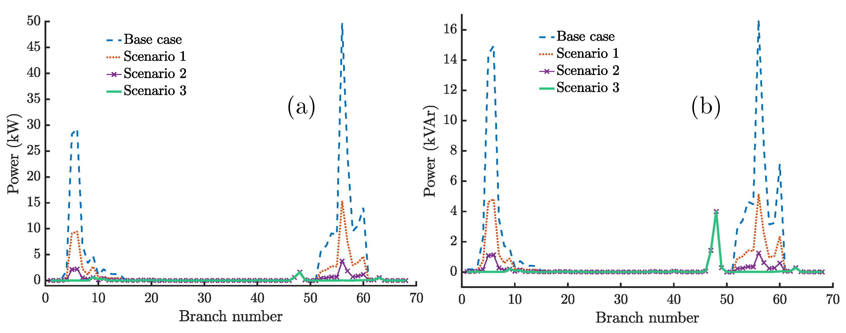
Figure 13 illustrates the branch active and reactive power losses for the IEEE 69-bus system under different scenarios using the RFO algorithm. Compared to the base case, all scenarios achieve significant reductions in loss. Among them, Scenario 3 demonstrates the most effective performance, resulting in the lowest losses across all scenarios. However, scenarios 2 and 3 exhibit peak reactive power losses at branch 48, indicating a localized concentration of reactive losses in these configurations.

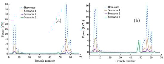
Figure 13. Branch (a) active and (b) reactive power losses for the IEEE 69-bus system under different scenarios using RFO.

Table 13 presents the maximum and minimum bus voltages along with their corresponding bus numbers, as well as the voltage deviation ($V_d$) across three different scenarios using various optimization techniques. The voltage limits are respected in all cases. Notably, the lowest voltage deviation is achieved in Scenario 3 using the RFO, RIME, and EEFO methods, which outperform the other techniques in terms of maintaining voltage profile consistency.

Table 13. The obtained voltages in pu after DGs installation for the IEEE 69-bus systems.

	Sc	RFO	RIME	EEFO	WOA	GA	SCA
	1	$0.9906474$ (65)	$0.9906823$ (65)	$0.9910402$ (65)	$0.9895067$ (65)	$0.9899228$ (65)	$0.9890661$ (65)
$V_{min}$ (at bus)	2	$0.9942436$ (50)	$0.9942437$ (50)	$0.9942436$ (50)	$0.9942438$ (50)	$0.9942390$ (50)	$0.9942488$ (50)
	3	$0.9942769$ (50)	$0.9942701$ (50)	$0.9942705$ (50)	$0.9942746$ (50)	$0.9943069$ (50)	$0.9942838$ (50)
	1	$1.000137$ (17)	1 (1)	$1.000216$ (17)	1 (1)	$1.000341$ (18)	$1.004606$ (14)
$V_{max}$ (at bus)	2	$1.000628$ (20)	$1.000743$ (19)	$1.000680$ (19)	$1.000573x$ (10)	$1.000997$ (24)	$1.003533$ (18)
	3	$1.001770$ (10)	$1.000950$ (61)	$1.000877$ (61)	$1.004669$ (61)	$1.003164$ (23)	$1.000413$ (21)
	1	$0.065612$	$0.065344$	$0.058766$	$0.084152$	$0.091385$	$0.1089x$
$V_d$(%)	2	$0.010818$	$0.010717$	$0.010815$	$0.020142$	$0.019968$	$0.021667$
	3	$0.0099357$	$0.0092931$	$0.0092067$	$0.025911$	$0.044316$	$0.027817$

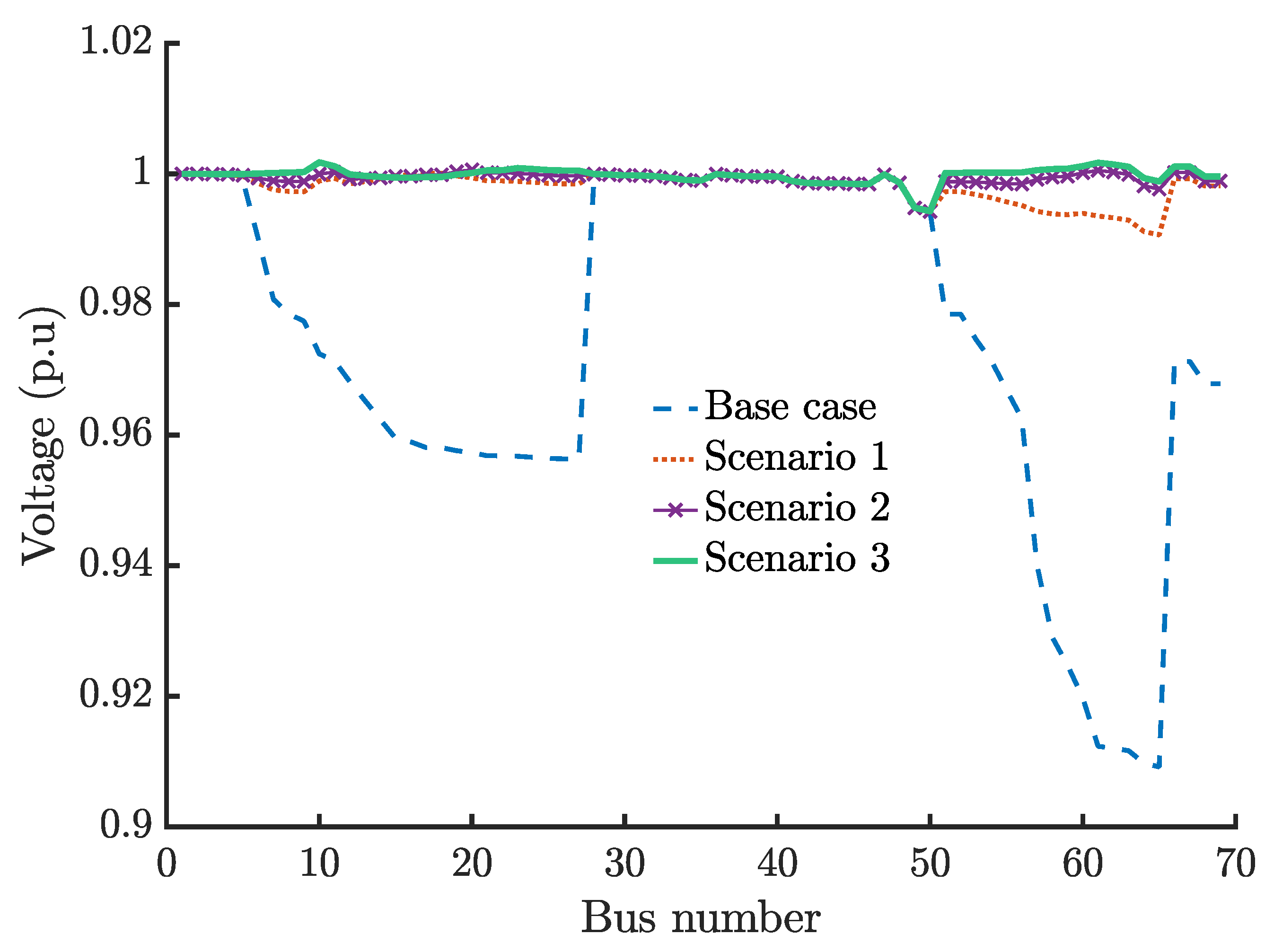
Figure 14 illustrates the bus voltage profiles for the IEEE 69-bus system under different scenarios using RFO. All scenarios significantly improve the voltage profile compared to the base case, with Scenario 3 providing the best overall voltage regulation across the network.

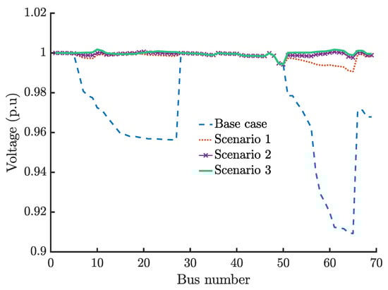
Figure 14. Bus voltage for the IEEE 69-bus system under different scenarios using RFO.

5. Conclusions and Future Work

In this paper, an effective Rüppell’s fox optimizer (RFO), along with five different metaheuristic algorithms, was employed to determine the optimal location, size, and power factor of PVDG and WTDG units in two IEEE distribution networks—one with thirty-three buses and the other with sixty-nine buses. The primary goal was to minimize power losses and enhance the voltage profile. The multi-objective function, composed of total active power loss and voltage deviation, was converted into a single-objective function using the weighted sum method.

The optimization problem was addressed under three different scenarios: the first assuming a unity power factor, the second assuming a power factor of $0.95$, and the third treating the power factor as a decision variable.

The results indicate that the third scenario consistently achieved the highest percentage of real and reactive power loss reduction across nearly all algorithms, along with the lowest maximum voltage deviation. Among the top-performing algorithms (RFO, RIME, and EEFO), the best active power loss reductions were approximately $94\%$ for the IEEE 33-bus system and $98\%$ for the IEEE 69-bus system. Similarly, the best reactive power loss reductions were about $92\%$ and $93\%$, respectively. The voltage deviation was also significantly improved, reaching as low as $0.02\%$ for the 33-bus system and $0.009\%$ for the 69-bus system.

Based on the findings of this study, several directions are proposed for future work to further enhance the optimization process and expand the scope of the analysis:

•

Explore the use of algorithms specifically designed for solving multi-objective optimization problems.

•

Reformulate the objective function to include power quality indices for a more comprehensive evaluation.

•

Extend the benchmarking suite to include a broader range of optimization algorithms, further validating RFO across diverse evolutionary computation frameworks.

•

Apply the proposed RFO approach to real-world or utility-scale distribution networks to enhance its practical applicability.

•

Conduct a sensitivity analysis on both the number and size of DG units to evaluate their impact on voltage profiles, power loss, and system reliability under varying loading and penetration levels.

References

- Akmal, M.; Umeh, O.; Yusuf, A.; Onyenagubom, A. Impact of Distributed Generation and Battery Energy Storage Systems on an Interconnected Power System. In Proceedings of the 2024 7th International Conference on Energy Conservation and Efficiency (ICECE), Lahore, Pakistan, 6–7 March 2024; IEEE: Piscataway, NJ, USA, 2024; pp. 1–6. [Google Scholar] [CrossRef]
- Hsu, W.; Chen, R.; Yang, Z.; Huang, C. Analysis of characteristics in motor failure of power system based on power spectral entropy. In Proceedings of the 2024 6th International Conference on Energy, Power and Grid (ICEPG), Guangzhou, China, 27–29 September 2024; IEEE: Piscataway, NJ, USA, 2024; pp. 1399–1402. [Google Scholar] [CrossRef]
- Kumar, N.; Mohapatra, A.; Bajpai, P. Linear Modified Distribution Power Flow Analysis. In Proceedings of the 2024 IEEE PES Innovative Smart Grid Technologies—Asia (ISGT Asia), Bengaluru, India, 10–13 November 2024; IEEE: Piscataway, NJ, USA, 2024; pp. 1–6. [Google Scholar] [CrossRef]
- Gallegos, J.; Arévalo, P.; Montaleza, C.; Jurado, F. Sustainable Electrification—Advances and Challenges in Electrical-Distribution Networks: A Review. Sustainability 2024, 16, 698. [Google Scholar] [CrossRef]
- Behbahani, M.R.; Jalilian, A.; Bahmanyar, A.; Ernst, D. Comprehensive Review on Static and Dynamic Distribution Network Reconfiguration Methodologies. IEEE Access 2024, 12, 9510–9525. [Google Scholar] [CrossRef]
- Lotfi, H.; Hajiabadi, M.E.; Parsadust, H. Power Distribution Network Reconfiguration Techniques: A Thorough Review. Sustainability 2024, 16, 10307. [Google Scholar] [CrossRef]
- Kahouli, O.; Alsaif, H.; Bouteraa, Y.; Ben Ali, N.; Chaabene, M. Power System Reconfiguration in Distribution Network for Improving Reliability Using Genetic Algorithm and Particle Swarm Optimization. Appl. Sci. 2021, 11, 3092. [Google Scholar] [CrossRef]
- Mahdavian, M.; Kafi, M.H.; Movahedi, A.; Janghorbani, M. Improve performance in electrical power distribution system by optimal capacitor placement using genetic algorithm. In Proceedings of the 2017 14th International Conference on Electrical Engineering/Electronics, Computer, Telecommunications and Information Technology (ECTI-CON), Phuket, Thailand, 27–30 June 2017; IEEE: Piscataway, NJ, USA, 2017; pp. 749–752. [Google Scholar] [CrossRef]
- Ufa, R.; Malkova, Y.; Rudnik, V.; Andreev, M.; Borisov, V. A review on distributed generation impacts on electric power system. Int. J. Hydrogen Energy 2022, 47, 20347–20361. [Google Scholar] [CrossRef]
- Magnusson, S.; Qu, G.; Li, N. Distributed Optimal Voltage Control With Asynchronous and Delayed Communication. IEEE Trans. Smart Grid 2020, 11, 3469–3482. [Google Scholar] [CrossRef]
- Aljendy, R.; Nasyrov, R.R.; Abdelaziz, A.Y.; Diab, A.A.Z. Enhancement of Power Quality with Hybrid Distributed Generation and FACTS Device. IETE J. Res. 2019, 68, 2259–2270. [Google Scholar] [CrossRef]
- Rajakumar, P.; Balasubramaniam, P.M.; Aldulaimi, M.H.; M, A.; Ramesh, S.; Alam, M.M.; Al-Mdallal, Q.M. An integrated approach using active power loss sensitivity index and modified ant lion optimization algorithm for DG placement in radial power distribution network. Sci. Rep. 2025, 15, 10481. [Google Scholar] [CrossRef] [PubMed]
- Mewafy, A.A.; Kaddah, S.S.; Eladawy, M. Multi-Objective Optimal DG Placement Approach Using Analytical Hierarchy Process. Electr. Power Compon. Syst. 2023, 51, 1648–1663. [Google Scholar] [CrossRef]
- Motling, B.; Paul, S.; Nee Dey, S.H. An Analytical Approach for Optimal DG Placement in Distribution Network Contaminated With Harmonics. In Proceedings of the 2022 IEEE Calcutta Conference (CALCON), Kolkata, India, 10–11 December 2022; IEEE: Piscataway, NJ, USA, 2022; pp. 212–217. [Google Scholar] [CrossRef]
- Roy, K.; Bansal, S.K.; Bansal, R.C. Performance enhancement of radial distribution system with optimal DG allocation. Int. J. Model. Simul. 2023, 45, 245–263. [Google Scholar] [CrossRef]
- Salimon, S.; Adepoju, G.; Adebayo, I.; Howlader, H.; Ayanlade, S.; Adewuyi, O. Impact of Distributed Generators Penetration Level on the Power Loss and Voltage Profile of Radial Distribution Networks. Energies 2023, 16, 1943. [Google Scholar] [CrossRef]
- Trivić, B.; Savić, A. Optimal Allocation and Sizing of BESS in a Distribution Network with High PV Production Using NSGA-II and LP Optimization Methods. Energies 2025, 18, 1076. [Google Scholar] [CrossRef]
- Khunkitti, S.; Boonluk, P.; Siritaratiwat, A. Optimal Location and Sizing of BESS for Performance Improvement of Distribution Systems with High DG Penetration. Int. Trans. Electr. Energy Syst. 2022, 2022, 6361243. [Google Scholar] [CrossRef]
- Khalil, M.A.; Elkhodragy, T.M.; Salem, W.A.A. A novel hybrid algorithm based on optimal size and location of photovoltaic with battery energy storage systems for voltage stability enhancement. Electr. Eng. 2024, 107, 1009–1034. [Google Scholar] [CrossRef]
- Ferminus Raj, A.; Gnana Saravanan, A. An optimization approach for optimal location & size of DSTATCOM and DG. Appl. Energy 2023, 336, 120797. [Google Scholar] [CrossRef]
- Dey, I.; Roy, P.K. Renewable DG allocation in radial distribution networks for techno-economic analysis using Chaotic Quasi Oppositional Arithmetic Optimization Algorithm. Measurement 2025, 249, 117012. [Google Scholar] [CrossRef]
- Ebrahimi, A.; Moradlou, M.; Bigdeli, M.; Mashhadi, M.R. Optimal sizing and allocation of PV-DG and DSTATCOM in the distribution network with uncertainty in consumption and generation. Discov. Appl. Sci. 2025, 7, 411. [Google Scholar] [CrossRef]
- Wanjekeche, T.; Ndapuka, A.A.; Mukena, L.N. Strategic Sizing and Placement of Distributed Generation in Radial Distributed Networks Using Multiobjective PSO. J. Energy 2023, 2023, 6678491. [Google Scholar] [CrossRef]
- Nasreddine, B.; Fethi, B.; Yassine, H.; Imane, H.; Riyadh, B. Optimal Sizing and Placement of Distributed Generation with Short-Circuit Analysis Using a Combined Technique Based on Modified PSO and ETAP. In Proceedings of the 2024 2nd International Conference on Electrical Engineering and Automatic Control (ICEEAC), Setif, Algeria, 12–14 May 2024; IEEE: Piscataway, NJ, USA, 2024; pp. 1–6. [Google Scholar] [CrossRef]
- Bendriss, B.; Sayah, S.; Hamouda, A. Efficient multi-objective optimization approach for solving optimal DG placement and sizing problem in distribution systems. J. Eng. Res. 2024. [Google Scholar] [CrossRef]
- Riaz, M.U.; Malik, S.A.; Daraz, A.; Alrajhi, H.; Alahmadi, A.N.M.; Afzal, A.R. Advanced Energy Management in a Sustainable Integrated Hybrid Power Network Using a Computational Intelligence Control Strategy. Energies 2024, 17, 5040. [Google Scholar] [CrossRef]
- Rehman, H.U.; Hussain, A.; Haider, W.; Ali, S.A.; Kazmi, S.A.A.; Huzaifa, M. Optimal Planning of Solar Photovoltaic (PV) and Wind-Based DGs for Achieving Techno-Economic Objectives across Various Load Models. Energies 2023, 16, 2444. [Google Scholar] [CrossRef]
- Al Igeb, B.H.; Al-Kaabi, M.; Oshchepkov, P.P.; Muhssin, M.; Abdulazeez, A.D. Grey Wolf Optimizer Algorithm to Solve Optimal Placement and Sizing of the Distributed Generation Sources in Distribution Radial Networks. In Proceedings of the 2023 International Symposium on Fundamentals of Electrical Engineering (ISFEE), Bucharest, Romania, 16–18 November 2023; IEEE: Piscataway, NJ, USA, 2023; pp. 1–6. [Google Scholar] [CrossRef]
- Alyu, A.B.; Salau, A.O.; Khan, B.; Eneh, J.N. Hybrid GWO-PSO based optimal placement and sizing of multiple PV-DG units for power loss reduction and voltage profile improvement. Sci. Rep. 2023, 13, 6903. [Google Scholar] [CrossRef] [PubMed]
- Chillab, R.K.; Jaber, A.S.; Smida, M.B.; Sakly, A. Optimal DG Location and Sizing to Minimize Losses and Improve Voltage Profile Using Garra Rufa Optimization. Sustainability 2023, 15, 1156. [Google Scholar] [CrossRef]
- Ayanlade, S.O.; Ariyo, F.K.; Jimoh, A.; Akindeji, K.T.; Adetunji, A.O.; Ogunwole, E.I.; Owolabi, D.E. Optimal Allocation of Photovoltaic Distributed Generations in Radial Distribution Networks. Sustainability 2023, 15, 13933. [Google Scholar] [CrossRef]
- Abbas, A.; Mun, T.; Lee, J.; Na, W.; Kim, J. Comparative study for various types of DG allocation for 24 hours load and generation profile. In Proceedings of the 2023 IEEE Energy Conversion Congress and Exposition (ECCE), Nashville, TN, USA, 29 October–2 November 2023; IEEE: Piscataway, NJ, USA, 2023; pp. 376–380. [Google Scholar] [CrossRef]
- Mondal, S.; De, M. Multi-Objective Optimal DG Allocation using Centrality Index and ABC Optimization for Three-phase UDS. In Proceedings of the 2022 2nd International Conference on Emerging Frontiers in Electrical and Electronic Technologies (ICEFEET), Patna, India, 24–25 June 2022; IEEE: Piscataway, NJ, USA, 2022; pp. 1–5. [Google Scholar] [CrossRef]
- Shirishti, S.; Gupta, A.R. Moth flame Optimisation based Allocation of DG and DSTATCOM in Radial Distribution System. In Proceedings of the 2022 2nd International Conference on Emerging Frontiers in Electrical and Electronic Technologies (ICEFEET), Patna, India, 24–25 June 2022; IEEE: Piscataway, NJ, USA, 2022; pp. 1–6. [Google Scholar] [CrossRef]
- Vellingiri, M.; Sivaraju, S. Optimal Placement and Sizing of Multiple DG Units using Improved Metaheuristic Algorithm on Transmission Systems. In Proceedings of the 2021 Third International Conference on Inventive Research in Computing Applications (ICIRCA), Coimbatore, India, 2–4 September 2021; IEEE: Piscataway, NJ, USA, 2021; pp. 251–256. [Google Scholar] [CrossRef]
- Gogula, S.; Vakula, V.S. Multi-objective Harris Hawks optimization algorithm for selecting best location and size of distributed generation in radial distribution system. Int. J. Cogn. Comput. Eng. 2024, 5, 436–452. [Google Scholar] [CrossRef]
- Chakraborty, S.; Verma, S.; Salgotra, A.; Elavarasan, R.M.; Elangovan, D.; Mihet-Popa, L. Solar-Based DG Allocation Using Harris Hawks Optimization While Considering Practical Aspects. Energies 2021, 14, 5206. [Google Scholar] [CrossRef]
- Khasanov, M.; Kamel, S.; Rahmann, C.; Hasanien, H.M.; Al-Durra, A. Optimal distributed generation and battery energy storage units integration in distribution systems considering power generation uncertainty. IET Gener. Transm. Distrib. 2021, 15, 3400–3422. [Google Scholar] [CrossRef]
- Su, H.; Zhao, D.; Heidari, A.A.; Liu, L.; Zhang, X.; Mafarja, M.; Chen, H. RIME: A physics-based optimization. Neurocomputing 2023, 532, 183–214. [Google Scholar] [CrossRef]
- Zhao, W.; Wang, L.; Zhang, Z.; Fan, H.; Zhang, J.; Mirjalili, S.; Khodadadi, N.; Cao, Q. Electric eel foraging optimization: A new bio-inspired optimizer for engineering applications. Expert Syst. Appl. 2024, 238, 122200. [Google Scholar] [CrossRef]
- Mirjalili, S.; Lewis, A. The Whale Optimization Algorithm. Adv. Eng. Softw. 2016, 95, 51–67. [Google Scholar] [CrossRef]
- Lambora, A.; Gupta, K.; Chopra, K. Genetic Algorithm—A Literature Review. In Proceedings of the 2019 International Conference on Machine Learning, Big Data, Cloud and Parallel Computing (COMITCon), Faridabad, India,, 14–16 February 2019; IEEE: Piscataway, NJ, USA, 2019; pp. 380–384. [Google Scholar] [CrossRef]
- Mirjalili, S. SCA: A Sine Cosine Algorithm for solving optimization problems. Knowl.-Based Syst. 2016, 96, 120–133. [Google Scholar] [CrossRef]
- Ghanbari, N.; Mokhtari, H.; Bhattacharya, S. Optimizing Operation Indices Considering Different Types of Distributed Generation in Microgrid Applications. Energies 2018, 11, 894. [Google Scholar] [CrossRef]
- Kayal, P.; Chanda, C. Placement of wind and solar based DGs in distribution system for power loss minimization and voltage stability improvement. Int. J. Electr. Power Energy Syst. 2013, 53, 795–809. [Google Scholar] [CrossRef]
- Bouali, Y.; Imarazene, K.; Berkouk, E.M. Total Harmonic Distortion Optimization of Multilevel Inverters Using Genetic Algorithm: Experimental Test on NPC Topology with Self-Balancing of Capacitors Voltage Using Multilevel DC-DC Converter. Arab. J. Sci. Eng. 2022, 48, 6067–6087. [Google Scholar] [CrossRef]
- Imarazene, K.; Bouali, Y.; Madjid Berkouk, E. Three-Level Space Vector PWM Implementation for Neutral Point Clamped Inverter using a Hardware Description Language. In Proceedings of the 2022 IEEE International Conference on Electrical Sciences and Technologies in Maghreb (CISTEM), Tunis, Tunisia, 26–28 October 2022; IEEE: Piscataway, NJ, USA, 2022; pp. 1–6. [Google Scholar] [CrossRef]
- Imarazene, K.; Bouali, Y.; Amani, M.; Berkouky, E.M. VHDL Implementation of Two-Level Space Vector PWM for FPGAs. In Proceedings of the 2022 2nd International Conference on Advanced Electrical Engineering (ICAEE), Constantine, Algeria, 29–31 October 2022; IEEE: Piscataway, NJ, USA, 2022; pp. 1–6. [Google Scholar] [CrossRef]
- Bouali, Y.; Imarazene, K.; Berkouk, E.M. Digital Control of PD-SPWM Algorithm for Three-Level Inverter Using FPGA Device. In Proceedings of the 2020 6th International Conference on Electric Power and Energy Conversion Systems (EPECS), Istanbul, Turkey, 5–7 October 2020; IEEE: Piscataway, NJ, USA, 2020; pp. 80–84. [Google Scholar] [CrossRef]
- Assouak, A.; Benabid, R. Setting and coordination of distance relays in interconnected power systems using DIgSILENT PowerFactory software. In Proceedings of the 2022 2nd International Conference on Advanced Electrical Engineering (ICAEE), Constantine, Algeria, 29–31 October 2022; IEEE: Piscataway, NJ, USA, 2022; pp. 1–5. [Google Scholar] [CrossRef]
- Braik, M.; Al-Hiary, H. Rüppell’s fox optimizer: A novel meta-heuristic approach for solving global optimization problems. Clust. Comput. 2025, 28, 292. [Google Scholar] [CrossRef]
- Gunantara, N. A review of multi-objective optimization: Methods and its applications. Cogent Eng. 2018, 5, 1502242. [Google Scholar] [CrossRef]
- Thangaraj, Y.; Kuppan, R. Multi-objective simultaneous placement of DG and DSTATCOM using novel lightning search algorithm. J. Appl. Res. Technol. 2017, 15, 477–491. [Google Scholar] [CrossRef]
Disclaimer/Publisher’s Note: The statements, opinions and data contained in all publications are solely those of the individual author(s) and contributor(s) and not of MDPI and/or the editor(s). MDPI and/or the editor(s) disclaim responsibility for any injury to people or property resulting from any ideas, methods, instructions or products referred to in the content. |
© 2025 by the authors. Licensee MDPI, Basel, Switzerland. This article is an open access article distributed under the terms and conditions of the Creative Commons Attribution (CC BY) license (https://creativecommons.org/licenses/by/4.0/).