A First-Order Autoregressive Process with Size-Biased Lindley Marginals: Applications and Forecasting

Abstract

In this paper, a size-biased Lindley (SBL) first-order autoregressive (AR(1)) process is proposed, the so-called SBL-AR(1). Some probabilistic and statistical properties of the proposed process are determined, including the distribution of its innovation process, the Laplace transformation function, multi-step-ahead conditional measures, autocorrelation, and spectral density function. In addition, the unknown parameters of the model are estimated via the conditional least squares and Gaussian estimation methods. The performance and behavior of the estimators are checked through some numerical results by a Monte Carlo simulation study. Additionally, two real-world datasets are utilized to examine the model’s applicability, and goodness-of-fit statistics are used to compare it to several pertinent non-Gaussian AR(1) models. The findings reveal that the proposed SBL-AR(1) model exhibits key theoretical properties, including a closed-form innovation distribution, multi-step conditional measures, and an exponentially decaying autocorrelation structure. Parameter estimation via conditional least squares and Gaussian methods demonstrates consistency and efficiency in simulations. Real-world applications to inflation expectations and water quality data reveal a superior fit over competing non-Gaussian AR(1) models, evidenced by lower values of the AIC and BIC statistics. Forecasting comparisons show that the classical conditional expectation method achieves accuracy comparable to some modern machine learning techniques, underscoring its practical utility for skewed and fat-tailed time series.

1. Introduction

Continuous-valued time series, in which realizations are continuously recorded over time, are useful in many domains, including engineering, economics, finance, and the natural sciences. In particular, they are employed in stock market analysis, scientific research, medical studies, economic forecasting, and weather forecasting. However, traditional time series analysis often assumes Gaussian-distributed marginals, which fail to capture the main features of real-world data, such as skewness, fat-tails, positivity, and size-biased sampling (e.g., environmental, economic, and biomedical data). For instance, Gaussian models cannot well accommodate strictly positive measurements like water turbidity or inflation rates, nor can they represent the high kurtosis observed in phenomena, such as financial volatility. These gaps limit their applicability and forecasting accuracy in non-Gaussian contexts. To address these limitations, several non-Gaussian AR(1) models have been proposed, highlighting some key features, e.g., skewness, fat tails, and positivity; among them are the gamma distribution (Gaver and Lewis [1]), Weibull and gamma (Sim [2]), exponential (Mališić [3]), inverse Gaussian (Abraham and Balakrishna [4]), normal-Laplace (Jose et al. [5]), approximated beta (Popović [6]), Lindley (Bakouch and Popovíc [7]), double Lindley (Nitha and Krishnarani [8]), gamma-Lindley (Mello et al. [9]), logistic (Jilesh and Jayakumar [10]), and exponential-Gaussian (Nitha and Krishnarani [11]).

From the distribution theory perspective, size-biased distributions, a special class of weighted distributions, emerge naturally in scenarios where observations are recorded with probabilities proportional to their inherent size or magnitude, a common feature in ecological surveys (e.g., oversampling large organisms), econometric data (e.g., prioritizing high-value transactions), or biomedical studies (e.g., detecting severe disease cases). These distributions address unequal detection probabilities inherent to real-world data collection, where larger or more prominent units (subjects) are systematically overrepresented. Their theoretical formulation, presented in weighting the original probability density function ($f\left(x\right)$) by the weight function x, called size-biased:

$$f_{SB}\left(x\right)={\displaystyle \frac{xf\left(x\right)}{E\left(X\right)}},x>0,$$

(1)

where the operator $E(.)$ is the expected value of a random variable X, as a normalizing factor, enables accurate modeling of such biased sampling mechanism. Pioneered by Patil and Rao [12], size-biased distributions have been extensively applied across environmental science, forestry, and social science, as demonstrated by Scheaffer [13] in wildlife population studies, Singh and Maddala [14] in econometric inequality analysis, and Drummer and McDonald [15] in ecological sampling. Beyond applied fields, size-biasing plays a pivotal role in statistical estimation, renewal theory, and distributional infinite divisibility. Despite their broad utility, their integration into non-Gaussian time series models remains limited, creating a critical gap in analyzing temporally dependent data subject to size-based sampling biases. This omission compromises parameter estimation and forecasting in fields like epidemiology (e.g., disease case reporting) or hydrology (e.g., extreme event monitoring), where detection probabilities inherently correlate with observation magnitude.

To contribute to this gap, we propose the size-biased Lindley AR(1) (SBL-AR(1)) process by using the size-biased Lindley (SBL) distribution introduced by Ayesha [16]. The SBL distribution enhances the classical Lindley, as non-Gaussian, distribution by incorporating size-biased sampling. Compared to other non-Gaussian distributions commonly used in time series models, such as double Lindley, gamma-Lindley and logistic, the size-biased Lindley distribution offers additional flexibility in capturing skewed and fat-tailed behaviors while inherently addressing size-biased sampling effects. This makes it particularly advantageous in applications. The probability density function (PDF), denoted as $f_{SBL}\left(x\right)$, and the cumulative distribution function (CDF), denoted as $F_{SBL}\left(x\right)$, of the SBL distribution are, respectively, given by

$$f_{SBL}(x;\theta )={\displaystyle \frac{{\theta }^{3}x(1+x)e^{-\theta x}}{2+\theta }},x>0,\theta >0,$$

$$F_{SBL}(x;\theta )=1-{\displaystyle \frac{(2+\theta +\theta x(2+\theta +\theta x))e^{-\theta x}}{2+\theta }},x>0,\theta >0,$$

where $\theta$ is a scale parameter of the SBL distribution.

The first two raw moments and the variance of the SBL distribution are, respectively, expressed as follows:

$$E\left(X\right)={\displaystyle \frac{2(\theta +3)}{\theta (\theta +2)}},$$

$$E\left(X^2\right)={\displaystyle \frac{6(\theta +4)}{{\theta }^2(\theta +2)}},$$

$$var\left(X\right)={\displaystyle \frac{2({\theta }^2+6\theta +6)}{{\theta }^2{(\theta +2)}^2}}.$$

For more details about the SBL distribution, see [16].

The limitations of traditional Gaussian time series models in capturing non-Gaussian features, previously stated, motivate the proposed SBL-AR(1) process, which integrates the SBL marginals to flexibly model positive-valued data with temporal dependence. The SBL-AR(1) addresses critical gaps in non-Gaussian autoregressive models through two key motivations: (1) SBL marginals, which enhance the classical Lindley distribution by weighting observations proportionally to their size, improving fit for data where larger values are oversampled (e.g., economic datasets), and (2) a closed-form innovation mixture combining Dirac delta and generalized gamma-exponential distributions, enabling precise modeling of excess zeros and continuous positive values. Parameter estimation via conditional least squares (CLS) and Gaussian estimation (GE) is validated through simulations demonstrating estimator consistency, while real-world applications, including inflation expectations and water turbidity monitoring, showcase a superior performance over competing models (e.g., Lindley, gamma, and inverse Gaussian AR(1)) via AIC/BIC criteria. By balancing theoretical findings (Laplace transformation function, multi-step-ahead conditional measures, autocorrelation decay, spectral density) with practical utility (accurate forecasting of skewed/fat-tailed data), the SBL-AR(1) establishes a flexible model for analyzing non-Gaussian time series prevalent in environmental and economic domains.

The remainder of this paper is constructed as follows: In Section 2, a first-order autoregressive process with SBL marginals is constructed, and the distribution of the innovation process is derived. Section 3 investigates some structural properties for the proposed SBL-AR(1), including multi-step conditional Laplace transform, conditional variance, conditional mean, autocorrelation function, and spectral density function. In Section 4, we utilize the conditional least squares and the Gaussian estimation techniques to estimate the parameters of the proposed process, and the performance of estimators is assessed via a simulation study. Section 5 discusses the application of the model using two real-life datasets. In addition, Section 6 gives the forecasting of the data for AR model based on the classical statistical method and some machine learning methods for its predictive ability. In Section 7, the paper’s conclusion provides suggestions for future research directions aligned with the proposed framework.

2. SBL-AR(1): Model Construction and Innovation Distribution

In this section, a first-order stationary autoregressive process with SBL marginals, denoted as SBLAR(1), is presented, and then we obtain the distribution of the innovation term.

Suppose that $\{X_t;t=1,2,\dots ,n\}$ is a stochastic process defined as follows:

$$X_t=\rho X_{t-1}+a_t,\rho \in [0,1)$$

(2)

where $\left\{X_t\right\}$ is a stationary process with SBL($\theta$) marginals, $\theta >0$, and $\left\{a_t\right\}$ is a sequence of independent and identically distributed (i.i.d.) random variables independent of $X_{t-s}$ for all $s\ge 1$. The definition of the SBL-AR(1) model indicates that it is a first-order Markovian process.

It is worth, before investigating more features for the SBL-AR(1) model, defining the generalized mixture distributions in the next definition.

Definition 1. 

Let $G\left(t\right)$ be a distribution function. $G\left(t\right)$ is said to be a generalized mixture of the distribution functions $G(t;1)$, $G(t;2),\dots$ if

$$G\left(t\right)=\sum _{i\ge 1}{\omega }_{i}G(t;i),$$

for all t, where ${\omega }_1$, ${\omega }_2,\dots$ are real numbers satisfying ${\sum }_{i\ge 1}{\omega }_i=1$, ${\sum }_{i\ge 1}\left|{\omega }_i\right|<\infty$, and for some indices i, ${\omega }_i<0$.

The following proposition gives the definition of the PDF, $h\left(x\right)$, which will be used later to find the innovation distribution. It is important to note that $h\left(x\right)$ is a properly PDF for all admissible values of the parameters $\rho$ and $\theta$.

Proposition 1. 

If $\theta \ge 1$, $x>0$, and $0<\rho <1$, then the generalized mixture

$$\begin{array}{ccc}\hfill h\left(x\right)& =& -{\displaystyle \frac{8(1-\rho ){\rho }^2}{\left(1-{\rho }^2\right){(\theta (1-\rho )+2)}^3}}\left({\displaystyle \frac{(\theta +2)}{\rho }}{e}^{-{\displaystyle \frac{(\theta +2)x}{\rho }}}\right)\hfill \\ & +& {\displaystyle \frac{2{(1-\rho )}^3}{\left(1-{\rho }^2\right)(\theta (1-\rho )+2)}}\left({\displaystyle \frac{1}{2}}{\theta }^3{x}^2{e}^{-\theta x}\right)\hfill \\ & +& {\displaystyle \frac{{(1-\rho )}^2(\theta (1-\rho )(\theta (1-\rho )+4\rho +2)+12\rho )}{\left(1-{\rho }^2\right){(\theta (1-\rho )+2)}^2}}\left({\theta }^{2}x{e}^{-\theta x}\right)\hfill \\ & +& {\displaystyle \frac{2\rho (1-\rho )\left(\theta (1-\rho )\left(\theta \left(-(1-\theta ){\rho }^2-2(\theta +2)\rho +\theta +5\right)+6(\rho +1)\right)+12\rho \right)}{\left(1-{\rho }^2\right){(\theta (1-\rho )+2)}^3}}\hfill \\ & \times & \left(\theta e^{-\theta x}\right)\hfill \end{array}$$

(3)

is a PDF.

Proof. 

Equation (3) combines exponential and gamma densities, which are non-negative, and represents a mixture of exponential $\left({\displaystyle \frac{\theta +2}{\rho }}\right)$, gamma $(3,\theta )$, gamma $(2,\theta )$, and exponential $\left(\theta \right)$, respectively. Therefore, it can be concluded that

$${\displaystyle {\int }_0^{\infty }}h\left(x\right)dx=1.$$

We still need to verify that $h\left(x\right)\ge 0$ for $x>0$. Equation (3) can be reformulated as follows:

$$h\left(x\right)={\displaystyle \frac{(1-\rho )}{(1-{\rho }^2)(\theta (1-\rho )+2)}}{e}^{-\theta x}{h}^{\ast }\left(x\right),$$

(4)

where

$$\begin{array}{ccc}\hfill h^{\ast }\left(x\right)& =& -{\displaystyle \frac{8{\rho }^2}{{(\theta (1-\rho )+2)}^2}}\left({\displaystyle \frac{(\theta +2)}{\rho }}{e}^{-{\displaystyle \frac{\left(\theta \right(1-\rho )+2)x}{\rho }}}\right)\hfill \\ & +& \left(2{(1-\rho )}^2\right)\left({\displaystyle \frac{1}{2}}{\theta }^3{x}^2\right)\hfill \\ & +& {\displaystyle \frac{(1-\rho )\left(\theta \right(1-\rho \left)\right(\theta (1-\rho )+4\rho +2)+12\rho )}{\left(\theta \right(1-\rho )+2)}}{\theta }^{2}x\hfill \\ & +& {\displaystyle \frac{2\rho \left(\theta (1-\rho )\left(\theta \left(-(1-\theta ){\rho }^2-2(\theta +2)\rho +\theta +5\right)+6(\rho +1)\right)+12\rho \right)}{{(\theta (1-\rho )+2)}^2}}\theta .\hfill \end{array}$$

(5)

As $\theta \ge 1$, we conclude that

$$\begin{array}{c}\hfill h^{\ast }\left(0\right)=2(\theta -1)(2+\theta (1-\rho ))\rho \ge 0.\end{array}$$

(6)

Additionally, we have that

$$\begin{array}{c}\hfill \underset{x\to \infty }{lim}{h}^{\ast }\left(x\right)=\infty ,\end{array}$$

(7)

and for $x>0$,

$$\begin{array}{ccc}\hfill {\left(h^{\ast }\left(x\right)\right)}^{\prime }& =& {\displaystyle \frac{8{\rho }^2}{{(\theta (1-\rho )+2)}^2}}\left({\displaystyle \frac{(\theta +2)}{\rho }}{\displaystyle \frac{\left(\theta \right(1-\rho )+2)}{\rho }}{e}^{-{\displaystyle \frac{\left(\theta \right(1-\rho )+2)x}{\rho }}}\right)\hfill \\ & +& \left(2{(1-\rho )}^2\right){\theta }^{3}x\hfill \\ & +& {\displaystyle \frac{(1-\rho )\left(\theta \right(1-\rho \left)\right(\theta (1-\rho )+4\rho +2)+12\rho )}{\left(\theta \right(1-\rho )+2)}}{\theta }^2>0.\hfill \end{array}$$

(8)

From Equations (6)–(8), $h^{\ast }\left(x\right)$ is a sum of non-negative terms due to $\theta \ge 1$ and derivative ${\left(h^{\ast }\left(x\right)\right)}^{\prime }>0$, ensuring that $h^{\ast }\left(x\right)\ge 0$, hence $h\left(x\right)\ge 0$ for $x>0$, which completes the proof.

That is, $h\left(x\right)$ represents a generalized mixture of the exponential (${\displaystyle \frac{\theta +2}{\rho }}$), gamma (2,$\theta$), gamma (3,$\theta$), and exponential ($\theta$) distributions such that the sum of weights in $h\left(x\right)$ is equal to 1. □

The distribution of the innovation sequence $\left\{a_t\right\}$ plays a crucial role in the practical applications and further studies of this process. One frequently used technique to determine the innovation sequence involves the Laplace transform function. The subsequent theorem presents the distribution of the innovation random variable (rv) $a_t$. Let ${\Phi }_{X_t}$ and ${\Phi }_{a_t}$ represent the Laplace transforms (LTs) of the random variables $X_t$ and $a_t$, respectively. The LT of SBL rv X can be expressed as

$${\Phi }_X\left(s\right)=E\left[e^{-sX}\right]={\displaystyle \frac{{\theta }^3(2+s+\theta )}{(2+\theta ){(s+\theta )}^3}}.$$

(9)

Theorem 1. 

Assume that $SBL\left(\theta \right)$ represents a marginal distribution of the stochastic process given by Equation (2). Consequently, the distribution of the innovation sequence, $\left\{a_t\right\}$, is a mixture of singular and absolutely continuous distributions, expressed as follows:

$$f_a\left(x\right)={\rho }^2\delta \left(x\right)+(1-{\rho }^2)h\left(x\right),$$

where $\delta \left(x\right)$ is the Dirac Delta function defined as

$$\delta \left(x\right)=\left\{\begin{array}{cc}\infty & x=0\\ 0& x\ne 0\end{array}\right.,$$

and $h\left(x\right)$ is given by Equation (3).

Proof. 

As the process $\left\{X_t\right\}$ is a stationary, the LT of Equation (2) can be expressed as

$$\begin{array}{ccc}\hfill {\Phi }_X\left(s\right)& =& {\Phi }_X\left(\rho s\right){\Phi }_a\left(s\right);\hfill \end{array}$$

consequently, the LT of the innovation rv $a_t$ is given by

$${\Phi }_a\left(s\right)={\displaystyle \frac{{\Phi }_X\left(s\right)}{{\Phi }_X\left(\rho s\right)}}.$$

(10)

By utilizing Equation (9), Equation (10) is represented as

$${\Phi }_a={\displaystyle \frac{(2+s+\theta ){(s\rho +\theta )}^3}{{(s+\theta )}^3(2+s\rho +\theta )}}.$$

(11)

By applying partial fraction decomposition, the preceding equation can be expressed as

$${\Phi }_a\left(s\right)={\rho }^2+(1-{\rho }^2)\left[A{\displaystyle \frac{2+\theta }{2+\theta +\rho s}}+B{\displaystyle \frac{{\theta }^3}{{(\theta +s)}^3}}+C{\displaystyle \frac{{\theta }^2}{{(\theta +s)}^2}}+D{\displaystyle \frac{\theta }{\theta +s}}\right],$$

where

$$\begin{array}{ccc}\hfill A& =& -{\displaystyle \frac{8(1-\rho ){\rho }^2}{\left(1-{\rho }^2\right){(\theta (1-\rho )+2)}^3}}=-{\displaystyle \frac{8{\rho }^2}{\left(1+\rho \right){(\theta (1-\rho )+2)}^3}},\hfill \end{array}$$

(12)

$$\begin{array}{ccc}\hfill B& =& {\displaystyle \frac{2{(1-\rho )}^3}{\left(1-{\rho }^2\right)(\theta (1-\rho )+2)}}={\displaystyle \frac{2{(1-\rho )}^2}{\left(1+\rho \right)(\theta (1-\rho )+2)}},\hfill \\ \hfill C& =& {\displaystyle \frac{{(1-\rho )}^2(\theta (1-\rho )(\theta (1-\rho )+4\rho +2)+12\rho )}{\left(1-{\rho }^2\right){(\theta (-\rho )+\theta +2)}^2}}\hfill \end{array}$$

(13)

$$\begin{array}{ccc}& =& {\displaystyle \frac{(1-\rho )\left(\theta \right(1-\rho \left)\right(\theta (1-\rho )+4\rho +2)+12\rho )}{\left(1+\rho \right){(\theta (-\rho )+\theta +2)}^2}},\hfill \end{array}$$

(14)

and

$$\begin{array}{ccc}\hfill D& =& {\displaystyle \frac{2\rho (1-\rho )\left(\theta (1-\rho )\left(\theta \left(-(1-\theta ){\rho }^2-2(\theta +2)\rho +\theta +5\right)+6(\rho +1)\right)+12\rho \right)}{\left(1-{\rho }^2\right){(\theta (1-\rho )+2)}^3}}\hfill \\ & =& {\displaystyle \frac{2\rho \left(\theta (1-\rho )\left(\theta \left(-(1-\theta ){\rho }^2-2(\theta +2)\rho +\theta +5\right)+6(\rho +1)\right)+12\rho \right)}{\left(1+\rho \right){(\theta (1-\rho )+2)}^3}}.\hfill \end{array}$$

(15)

It can be seen that ${\Phi }_a\left(0\right)={\displaystyle \frac{(2+\theta ){\theta }^3}{{\theta }^3(2+\theta )}}=1.$

Based on Equations (12)–(15) and the properties of inverse LTs, we conclude that the distribution of the innovation sequence, $\left\{a_t\right\}$, is composed of a discrete component of 0, with probability ${\rho }^2$, and a generalized mixture of exponential (${\displaystyle \frac{2+\theta }{\rho }}$), gamma (3, $\theta$), gamma (2, $\theta$), and exponential ($\theta$) distributions, with probability $1-{\rho }^2$. □

Figure 1 depicts the distribution of the innovation process through its density curves. From Figure 1a, it is clear that, as $\rho$ increases in the interval (0, 0.5), the values of the innovation probability increase, while in the case where $0.5\le \rho <1$, the values of the innovation probability decrease. Furthermore, plots in Figure 1b,c indicate that smaller $\theta$ values lead to distributions with heavier tails. In summary, the innovation density is both uni-modal and right-skewed.

Figure 1. Density curves for the innovation process $a_t=I_t{\epsilon }_t$: (a) $\theta$ = 1.5, (b) $\rho$ = 0.97, (c) $\rho$ = 0.2.

As a result of the previously mentioned theorem about the distribution of the innovation term, the stationary process $\left\{X_t\right\}$ in Equation (2) can be reformulated as follows.

Definition 2. 

The SBL-AR(1) process $\left\{X_t\right\}$ in Equation (2) is restated as

$$\begin{array}{c}\hfill X_t=\left\{\begin{array}{cc}\rho X_{t-1},& withprobability{\rho }^2\\ \rho X_{t-1}+{\epsilon }_t,& withprobability1-{\rho }^2.\end{array}\right.\end{array}$$

(16)

Or, in other terms,

$$X_t=\rho X_{t-1}+I_t{\epsilon }_t,$$

(17)

where $I_t$ is an indicator variable such that $P(I_t=0)=1-P(I_t=1)={\rho }^2$.

Figure 2 depicts the sample paths from the process in Equation (16) for different values of the parameters $\theta$ and $\rho$. We generated 200 observations from the SBL-AR(1) process by setting $\theta$ = 1.6, 2, and 2.5; and $\rho$ = 0.2, 0.5, and 0.7. Throughout these plots, the SBL-AR(1) behavior is investigated and Figure 2 points out that the simulated series is stationary and has positive values.

Figure 2. The sampling paths of the SBL-AR(1) process for (A) $\theta =1.6$, $\rho =0.2$, (B) $\theta =2$, $\rho =0.2$, (C) $\theta =2.5$, $\rho =0.5$, (D) $\theta =2.5$, $\rho =0.7$.

3. Structural Properties Associated with the SBL-AR(1) Model

This section focuses on the development of the SBL-AR(1) model’s conditional mean and variance, along with the derivation of its multi-step-ahead conditional Laplace transform. The mean and variance are required to establish the SBL-AR(1) prediction equations, while the Laplace transform provides insight into the joint distribution of vectors produced by the process. In this section, we outline some statistical properties of the SBL-AR(1) model and discuss each one in detail. The conditional statistical measures of the SBL-AR(1) process are obtained using the same methodology as outlined by Bakouch and Popović [7].

3.1. Some Statistical Conditional Measures

The one- and multi-step-ahead conditional mean and variance of the SBL-AR process are based on the mean and variance of the random variable ${\epsilon }_t$ and the innovation term $a_t$. Thus, we first compute the mean and variance for ${\epsilon }_t$ and $a_t$, respectively, as follows. According to the definition of the SBL-AR(1) process outlined in Equation (16), the random variable ${\epsilon }_t$ has the following mean and variance, respectively:

$$\begin{array}{ccc}\hfill E\left({\epsilon }_t\right)& =& {\displaystyle \frac{1}{1+\rho }}E\left(X_t\right)={\displaystyle \frac{1}{1+\rho }}{\displaystyle \frac{2(\theta +3)}{\theta (\theta +2)}},\hfill \end{array}$$

(18)

$$\begin{array}{ccc}\hfill Var\left({\epsilon }_t\right)& =& {\displaystyle \frac{2\left[6+12\rho -12{\rho }^2+{\theta }^2(1+2\rho -{\rho }^2)-6\theta (-1-2\rho +{\rho }^2)\right]}{{\theta }^2{(2+\theta )}^2{(1+\rho )}^2}}.\hfill \end{array}$$

(19)

Consequently, the mean and variance of the innovation process $a_t=I_t{\epsilon }_t$ are, respectively, stated as

$$E\left(a_t\right)=(1-\rho ){\displaystyle \frac{2(\theta +3)}{\theta (\theta +2)}},$$

(20)

$$Var\left(a_t\right)=(1-{\rho }^2){\displaystyle \frac{2({\theta }^2+6\theta +6)}{{\theta }^2{(\theta +2)}^2}}.$$

(21)

By utilizing these properties, the one-step ahead conditional mean for the process in Equation (16) can be formulated as

$$E\left(X_t\right|X_{t-1}=x_{t-1})=\rho x_{t-1}+E\left(I_t{\epsilon }_t\right)=\rho x_{t-1}+(1-\rho ){\displaystyle \frac{2(\theta +3)}{\theta (\theta +2)}}.$$

(22)

Consequently, the formula for the ($k+1$)-step ahead conditional mean is expressed as

$$E\left(X_{t+k}\right|X_{t-1}=x_{t-1})={\rho }^{k+1}{x}_{t-1}+(1-{\rho }^{k+1}){\displaystyle \frac{2(\theta +3)}{\theta (\theta +2)}}.$$

(23)

When $k\to \infty ,$ the previously mentioned expression will tend to the unconditional mean of the main process as follows:

$$E\left(X_{t+k}\right|X_{t-1}=x_{t-1})\to {\displaystyle \frac{2(\theta +3)}{\theta (\theta +2)}}.$$

The expressions for one-step and ($k+1$)-step-ahead conditional variance of the proposed model, respectively, are obtained as

$$Var\left(X_t\right|X_{t-1}=x_{t-1})=(1-{\rho }^2){\displaystyle \frac{2({\theta }^2+6\theta +6)}{{\theta }^2{(\theta +2)}^2}},$$

(24)

$$Var\left(X_{t+k}\right|X_{t-1}=x_{t-1})=(1-{\rho }^{2(k+1)}){\displaystyle \frac{2({\theta }^2+6\theta +6)}{{\theta }^2{(\theta +2)}^2}}.$$

(25)

Observe that when $k\to \infty$ in Equation (25), the unconditional variance of the main process is obtained as

$$Var\left(X_{t+k}\right|X_{t-1}=x_{t-1})\to {\displaystyle \frac{2({\theta }^2+6\theta +6)}{{\theta }^2{(\theta +2)}^2}}.$$

The multi-step-ahead conditional LT of the SBL-AR(1) process is obtained as

$$\begin{array}{ccc}\hfill {\Phi }_{X_{t+k}|X_{t-1}=x_{t-1}}\left(s\right)& =& E\left[e^{-s{X}_{t+k}}|X_{t-1}=x_{t-1}\right]\hfill \\ \\ & =& E\left[e^{-s\left({\rho }^{k+1}{X}_{t-1}+{\displaystyle {\sum }_{i=0}^k}{\rho }^{k-i}{a}_{k+i}\right)}|X_{t-1}=x_{t-1}\right]\hfill \\ & =& e^{-s{\rho }^{k+1}{x}_{t-1}}{\displaystyle \prod _{i=0}^k}{\Phi }_a\left({\rho }^{k-i}s\right)\hfill \\ \\ & =& e^{-s{\rho }^{k+1}{x}_{t-1}}{\displaystyle \prod _{i=0}^k}{\displaystyle \frac{(2+\theta +s{\rho }^{k-i}){(s{\rho }^{k+1-i}+\theta )}^3}{{(s{\rho }^{k-i}+\theta )}^3(2+\theta +s{\rho }^{k+1-i})}}\hfill \\ \\ & =& e^{-s{\rho }^{k+1}{x}_{t-1}}{\displaystyle \frac{(2+\theta +s){(s{\rho }^{k+1}+\theta )}^3}{{(s+\theta )}^3(2+\theta +s{\rho }^{k+1})}}.\hfill \end{array}$$

As $k\to \infty$, we obtain

$${\Phi }_{X_{t+k}|X_{t-1}=x_{t-1}}\left(s\right)\to {\displaystyle \frac{{\theta }^3(2+\theta +s)}{(2+\theta ){(s+\theta )}^3}}.$$

(26)

Noting that the final Equation (26) is equivalent to Equation (9), the unconditional LT of the process $\left\{X_t\right\}$.

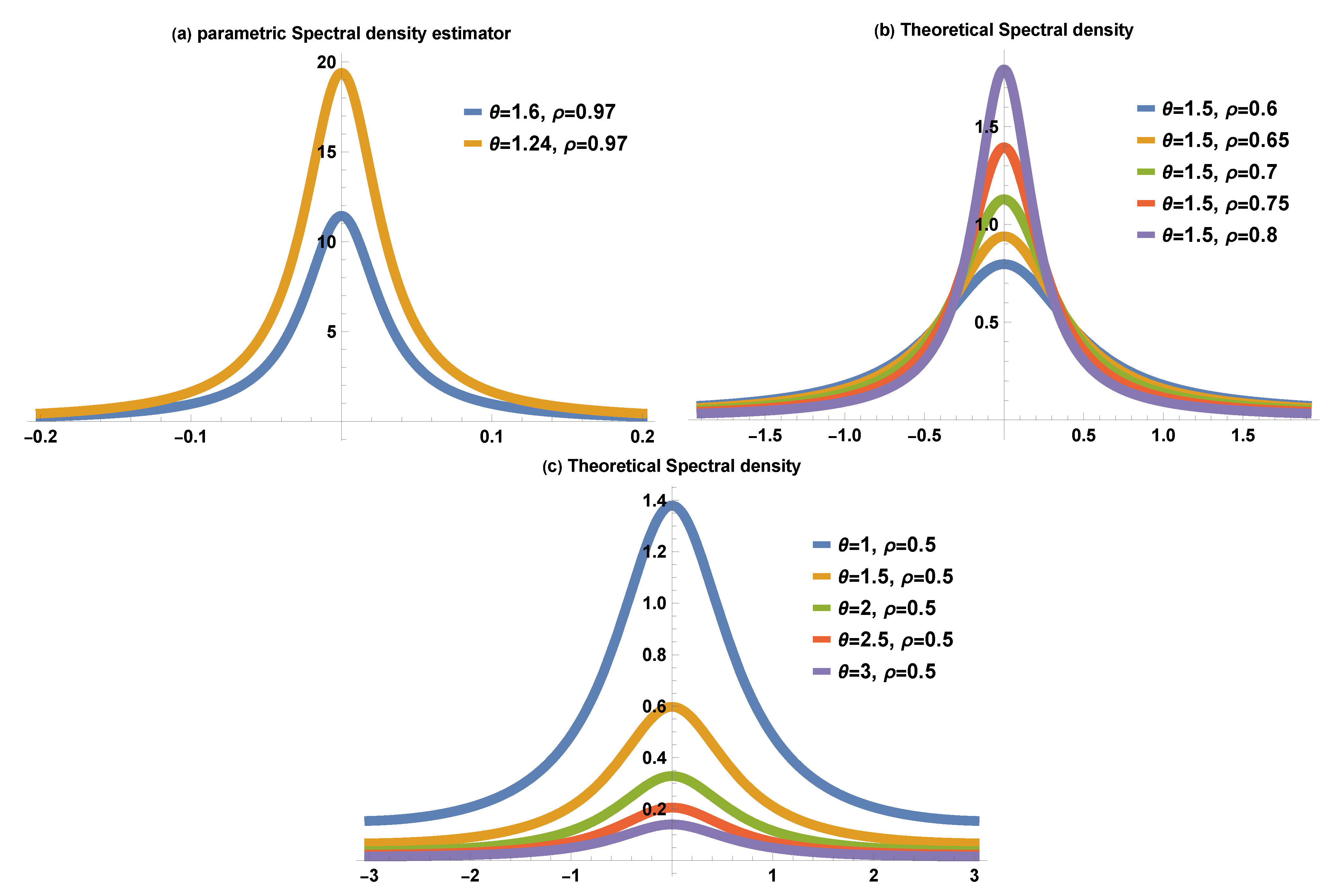
3.2. Joint Distribution, Autocorrelation, and Spectral Density Function

The joint LT of ($X_{t-1},X_t$) is expressed as follows:

$$\begin{array}{ccc}\hfill {\Phi }_{X_{t-1},X_t}(s_1,s_2)& =& E\left[e^{-s_1{X}_{t-1}-s_2{X}_t}\right]\hfill \\ \\ & =& E\left[e^{-s_1{X}_{t-1}-s_2(\rho X_{t-1}+a_t)}\right]\hfill \\ \\ & =& {\Phi }_X(s_1+s_2\rho ){\Phi }_a\left(s_2\right)\hfill \\ \\ & =& {\displaystyle \frac{{\theta }^3(2+\theta +(s_1+s_2\rho ))}{(2+\theta ){((s_1+s_2\rho )+\theta )}^3}}.{\displaystyle \frac{(2+s_2+\theta ){(s_2\rho +\theta )}^3}{{(s_2+\theta )}^3(2+s_2\rho +\theta )}}.\hfill \end{array}$$

The SBL-AR(1) process is not time reversible because the joint LT ${\Phi }_{X_{t-1},X_t}(s_1,s_2)$ is not symmetric in $s_1$ and $s_2$.

Following a few basic calculations, the autocovariance and autocorrelation functions at lag k of the proposed process are, respectively, given by

$$\begin{array}{ccc}\hfill \gamma \left(k\right)& =& {\rho }^{\left|k\right|}var\left(X_t\right)={\rho }^{\left|k\right|}{\displaystyle \frac{2({\theta }^2+6\theta +6)}{{\theta }^2{(\theta +2)}^2}},\hfill \end{array}$$

$$\eta \left(k\right)={\rho }^{\left|k\right|}.$$

The spectral density function of a stationary process is simply defined as the Fourier transform of the absolutely summable autocovariance function. Hence, the spectral density function of the SBL-AR(1) is obtained as follows:

$$f_X\left(w\right)={\displaystyle \frac{1}{2\pi }}{\displaystyle \sum _{z=-\infty }^{\infty }}\gamma \left(z\right)e^{-iwz},w\in [-\pi ,\pi ].$$

Given that ${\displaystyle \sum _{z=-\infty }^{\infty }}\left|\gamma \left(z\right)\right|<\infty$, by substituting $\gamma \left(z\right)$ in the last equation we obtain

$$f_X\left(w\right)={\displaystyle \frac{({\theta }^2+6\theta +6)(1-{\rho }^2)}{\pi {\theta }^2{(\theta +2)}^2(1+{\rho }^2-2\rho cosw)}}.$$

(27)

The parametric spectral density estimator is obtained by replacing the parameters $\theta$ and $\rho$ with their corresponding Gaussian estimators ${\widehat{\theta }}_{GE}$ and ${\widehat{\rho }}_{GE}$, which will be discussed later, in the right hand side of Equation (27).

Figure 3a displays the spectral density function estimator of the SBL-AR(1) process that is given by Equation (27) for ${\widehat{\theta }}_{GE}=1.24,1.6$, and ${\widehat{\rho }}_{GE}=0.97$, where those estimated values will be obtained later in Section 5. Figure 3b depicts the theoretical SBL-AR(1) spectral density function at $\theta =1.5$ and different values for $\rho$. As the value of $\rho$ increases, the spectral density function becomes more leptokurtic. Also, from Figure 3c, it is clear that at $\rho$ = 0.5 and various $\theta$ values, the spectral density function becomes more platykurtic as $\theta$ increases. Further, curves in Figure 3a are very similar to ones in Figure 3b.

Figure 3. Spectral density curves of SBL-AR(1) process: (a) $\rho =0.97$, (b) $\theta =1.5$, and (c) $\rho =0.5$.

4. Parameter Estimation and Simulation Studies

This section is devoted to estimating the parameters involved in the process, specifically $\rho$ and $\theta$. Let $(X_1,X_2,\dots ,X_n)$ represent a realization from the SBL-AR(1) process. The next subsections discuss the conditional least squares and the Gaussian estimation techniques. Additionally, a simulation study will be performed.

4.1. Estimation via Conditional Least Squares Procedure

The conditional least squares (CLS) estimators for $\rho$ and $\theta$, denoted as ${\widehat{\rho }}_{CLS}$ and ${\widehat{\theta }}_{CLS}$, are derived by minimizing the conditional sum of squares function

$$\begin{array}{ccc}\hfill Q_n(\rho ,\theta )& =& {\displaystyle \sum _{t=2}^n}{\left(X_t-E\left(X_t|X_{t-1}\right)\right)}^2.\hfill \end{array}$$

By utilizing Equation (22) for $E\left(X_t|X_{t-1}\right)$, then $Q_n(\rho ,\theta )$ takes the form

$$\begin{array}{ccc}\hfill Q_n(\rho ,\theta )& =& {\displaystyle \sum _{t=2}^n}{\left(X_t-\rho X_{t-1}-(1-\rho ){\displaystyle \frac{2(\theta +3)}{\theta (\theta +2)}}\right)}^2.\hfill \end{array}$$

Consequently, by setting ${\displaystyle \frac{2(\theta +3)}{\theta (\theta +2)}}={\mu }_X$, then the previous equation can rewritten as

$$\begin{array}{ccc}\hfill Q_n(\rho ,\theta )& =& {\displaystyle \sum _{t=2}^n}{\left(X_t-\rho X_{t-1}-(1-\rho ){\mu }_X\right)}^2.\hfill \end{array}$$

(28)

Estimating $\rho$ and ${\mu }_X$ is achieved by solving the normal equations obtained from Equation (28), which are as follows:

$${\widehat{\rho }}_{CLS}={\displaystyle \frac{(n-1){\displaystyle \sum _{t=2}^n}{X}_t{X}_{t-1}-{\displaystyle \sum _{t=2}^n}{X}_t{\displaystyle \sum _{t=2}^n}{X}_{t-1}}{(n-1){\displaystyle \sum _{t=2}^n}{\displaystyle X_{t-1}^2}-{\left({\displaystyle \sum _{t=2}^n}{X}_{t-1}\right)}^2}},$$

(29)

$${\widehat{\mu }}_{X_{CLS}}={\displaystyle \frac{{\displaystyle \sum _{t=2}^n}{X}_t-\widehat{\rho }{\displaystyle \sum _{t=2}^n}{X}_{t-1}}{(n-1)(1-\widehat{\rho })}}.$$

(30)

As ${\mu }_X={\displaystyle \frac{2(\theta +3)}{\theta (\theta +2)}}$, then the estimator for $\theta$ is obtained as

$$\begin{array}{c}\hfill {\widehat{\theta }}_{CLS}={\displaystyle \frac{-({\widehat{\mu }}_{X_{CLS}}-1)+\sqrt{{({\widehat{\mu }}_{X_{CLS}}-1)}^2+6{\widehat{\mu }}_{X_{CLS}}}}{{\widehat{\mu }}_{X_{CLS}}}},\end{array}$$

(31)

where ${\widehat{\mu }}_{X_{CLS}}$ is given by Equation (30).

4.2. Gaussian Estimation Approach

Whittle [17] proposed this approach by utilizing the Gaussian likelihood function as the baseline distribution for estimation. Subsequently, Crowder [18] applied this estimation technique to analyze correlated binomial data. Both Al-Nachawati et al. [19] and Alwasel et al. [20] employed the same estimation technique within the context of a first-order autoregressive process. Despite its approximate nature, this method provides a reliable estimation for the proposed model. The Gaussian estimation (GE) approach is based on the one-step conditional expectation and variance of the model. The conditional maximum likelihood function is expressed as follows:

$$L(\rho ,\theta )=f\left(x_1\right){\displaystyle \prod _{t=2}^n}f\left(x_t\right|x_{t-1}).$$

In this context, $f\left(x_t\right|x_{t-1})$ and $f\left(x_1\right)$ represent the conditional and marginal probability functions of $X_t|X_{t-1}$ and $X_t$, respectively. We assume that both $f\left(x_t\right|x_{t-1})$ and $f\left(x_1\right)$ follow a Gaussian PDF, with the conditional mean and conditional variance serving as their parameters. Thus, the likelihood function can be formulated as follows:

$$L(\rho ,\theta )={\left(2\pi \right)}^{{\displaystyle \frac{-n}{2}}}{\left({\displaystyle {\sigma }_{x_{t-1}}^2}\right)}^{{\displaystyle \frac{-n}{2}}}exp\left[{\displaystyle \sum _{t=2}^n}{\displaystyle \frac{-{\left(x_t-{\mu }_{x_{t-1}}\right)}^2}{2{\displaystyle {\sigma }_{x_{t-1}}^2}}}\right].$$

Consequently, the log-likelihood function is given by

$$\begin{array}{ccc}\hfill l(\rho ,\theta )& =& log\left(L(\rho ,\theta )\right)={\displaystyle \frac{-n}{2}}log\left(2\pi \right)-{\displaystyle \frac{1}{2}}{\displaystyle \sum _{t=2}^n}\left({\displaystyle \frac{{\left(x_t-{\mu }_{x_{t-1}}\right)}^2}{{\displaystyle {\sigma }_{x_{t-1}}^2}}}+log\left({\displaystyle {\sigma }_{x_{t-1}}^2}\right)\right),\hfill \end{array}$$

where ${\mu }_{x_{t-1}}=E\left(X_t\right|X_{t-1}=x_{t-1})$ and ${\displaystyle {\sigma }_{x_{t-1}}^2}=Var\left(X_t\right|X_{t-1}=x_{t-1})$ are the one-step conditional mean and variance defined by Equation (22) and Equation (24), respectively. Hence, the Gaussian log-likelihood function related to the SBL-AR(1) process takes the form   

$$\begin{array}{ccc}\hfill l(\rho ,\theta )& =& {\displaystyle \frac{-n}{2}}log\left(2\pi \right)-{\displaystyle \frac{1}{2}}{\displaystyle \sum _{t=2}^n}\left\{log\left({\displaystyle \frac{(1-{\rho }^2)\left(2({\theta }^2+6\theta +6)\right)}{{\theta }^2{(\theta +2)}^2}}\right)\right.\hfill \\ & +& \left.{\displaystyle \frac{{\theta }^2{(\theta +2)}^2}{(1-{\rho }^2)\left(2({\theta }^2+6\theta +6)\right)}}{\left(x_t-\rho x_{t-1}-(1-\rho ){\displaystyle \frac{2(\theta +3)}{\theta (\theta +2)}}\right)}^2\right\}.\hfill \end{array}$$

(32)

Therefore, the Gaussian estimators, termed ${\widehat{\rho }}_{GE}$ and ${\widehat{\theta }}_{GE}$, can be derived by solving the system of equations ${\displaystyle \frac{\partial l(\rho ,\theta )}{\partial \rho }}=0$ and ${\displaystyle \frac{\partial l(\rho ,\theta )}{\partial \theta }}=0$.

Crowder [18] indicated that when employing the Gaussian method for estimating the parameter $\Omega$, the expression $\sqrt{n}(\widehat{\Omega }-\Omega )$ is asymptotically normally distributed with a mean of zero and an asymptotic variance of ${\left[J(\Omega )\right]}^{-1}$, where $J(\Omega )$ denotes the conditional expected information matrix. An approximation can be achieved using the observed conditional information matrix, as discussed by Bakouch and Popović [7].

Now, we conduct a simulation study in the next subsection to check the performance of the CLS and GE estimation methods.

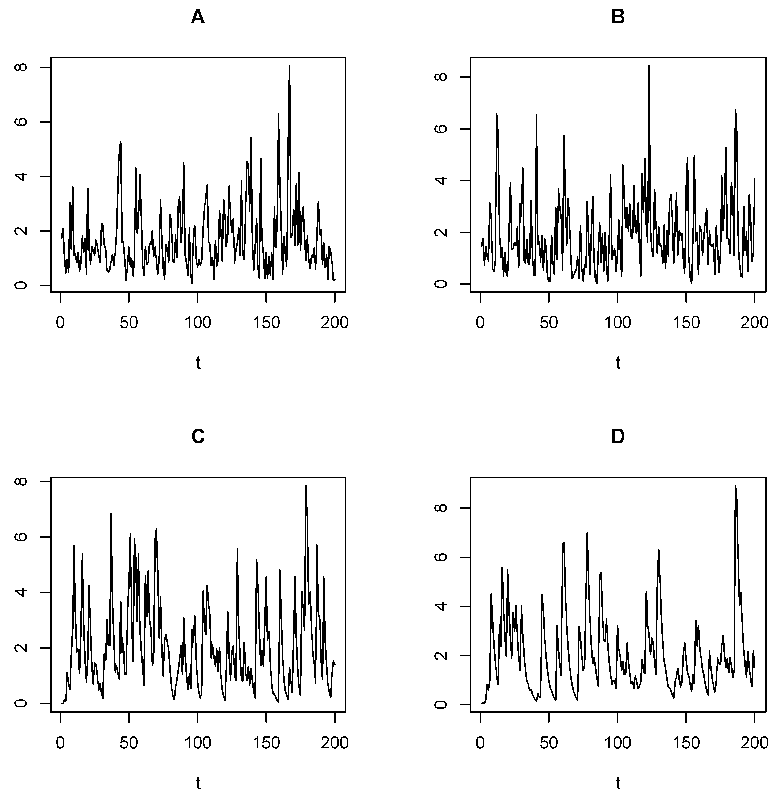
4.3. Monte Carlo Simulation and Experimental Analysis

In this subsection, we perform a simulation study to check the validity of the estimation methods, which are used for the model parameters’ estimation. The consistency and behavior of the CLS and GE techniques of parameter estimation in the SBL-AR(1) process are investigated throughout a Monte Carlo simulation. Over 1000 replications and sample sizes of 50, 100, 500, and 1000 are simulated from the SBL-AR(1) with actual parameter values:

• (a) $\rho =0.97,\theta =1.24,$   (b) $\rho =0.97,\theta =1.6,$
• (c) $\rho =0.5,\theta =1.4,$   (d) $\rho =0.7,\theta =1.4,$
• (e) $\rho =0.1,\theta =1.5,$   (f) $\rho =0.5,\theta =1.5.$

The mean square error (MSE) is used to assess the performance of the estimates and comparison purposes.

A step-by-step simulation algorithm for the SBL-AR(1) process is provided as follows (Algorithm 1):

Algorithm 1: Simulation algorithm for the SBL-AR(1) process

1. Specify the values for the parameters $\rho$, $\theta$, sample size (n) and the number of iterations ($N=1000$). 2. Compute the innovation random variable $a_t(=I_t{\epsilon }_t)$, where $I_t$ follows a Bernoulli distribution with parameter $1-{\rho }^2$, and $I_t{\epsilon }_t$ is a mixture of exponential and gamma distributions, generated using rexp and rgamma functions. 3. Simulate the SBL-AR(1) process using the relation in Equation (17). 4. For each generated sample size, the parameters are estimated using (GE) via the optim function in R, which maximizes the likelihood in Equation (32), along with the CLS approach outlined in Equations (29) and (31). 5. Repeat steps for $n=50,100,500$ and 1000. 6. Compute the average of the estimates, biases, and the MSE.

The values of $\rho$ and $\theta$ used in the simulation study were subject to the constraints $\theta \ge 1$ and $0<\rho <1$. Notably, some of these values correspond to the parameter estimates obtained from the real-world datasets analyzed in this study.

Table 1 and Table 2 display the values for the mean estimates, bias, and MSE. The bias and MSE are provided in the parentheses as (bias, MSE). Generally, both approaches performed well and effectively. In the two methodologies, the bias and MSE for all estimates tended to zero as the sample size increased. Additionally, when the sample size was increased, the values of the estimate became closer to the actual values. In terms of MSE and the values of mean estimates, the GE outperformed the CLS for ($\rho ,\theta$) = (0.1, 1.5), (0.97, 1.24), (0.97, 1.6), (0.5, 1.4), and (0.7, 1.4). However, the CLS showed better performance for ($\rho ,\theta$) = (0.5, 1.5).

Table 1. Average, bias, and MSE (in parentheses) of the estimates for some different values of the parameters $\rho$ and $\theta$.

Scenarios	n	${\widehat{\mathit{\rho }}}_{\mathit{CLS}}$	${\widehat{\mathit{\theta }}}_{\mathit{CLS}}$	${\widehat{\mathit{\rho }}}_{\mathit{GE}}$	${\widehat{\mathit{\theta }}}_{\mathit{GE}}$
(a) ($\rho ,\theta$) = (0.97, 1.24)
	50	0.905966	1.467342	0.976374	1.251286
		(−0.064034, 0.008183)	(0.227342, 0.344839)	(0.007344, 0.000575)	(0.012526, 0.021865)
	100	0.93888	1.446866	0.975805	1.262123
		(−0.03112, 0.002239)	(0.206866, 0.248877)	(0.006775, 0.000366)	(0.023363, 0.019913)
	500	0.963309	1.401944	0.977312	1.2481
		(−0.006691, 0.000184)	(0.161944, 0.062201)	(0.008282, 0.000164)	(0.00934, 0.004442)
	1000	0.966316	1.287918	0.977207	1.249197
		(−0.003684, 0.000082)	(0.047918, 0.010303)	(0.008177, 0.00012)	(0.010437, 0.002362)
(b) ($\rho ,\theta$) = (0.97, 1.6)
	50	0.904868	1.743993	0.973699	1.589438
		(−0.065132, 0.009001)	(0.143993, 0.465764)	(0.004669, 0.000633)	(−0.008962, 0.030876)
	100	0.939137	1.731105	0.975531	1.601991
		(−0.030863, 0.002211)	(0.131105, 0.31464)	(0.006501, 0.000409)	(0.003591, 0.027661)
	500	0.962916	1.695561	0.974227	1.596723
		(−0.007084, 0.000178)	(0.095561, 0.062953)	(0.005197, 0.000148)	(−0.001677, 0.00524)
	1000	0.966588	1.626271	0.974214	1.597994
		(−0.003412, 0.00008)	(0.026271, 0.01708)	(0.005184, 0.000096)	(−0.000406, 0.001813)
(c) ($\rho ,\theta$) = (0.5, 1.4)
	50	0.468009	1.607588	0.465563	1.565282
		(−0.031991, 0.015481)	(0.207588, 0.128041)	(−0.033937, 0.013012)	(0.166682, 0.110757)
	100	0.480446	1.594822	0.468969	1.513646
		(−0.019554, 0.007864)	(0.194822, 0.073287)	(−0.030531, 0.006731)	(0.115046, 0.052598)
	500	0.493206	1.569898	0.479231	1.477341
		(−0.006794, 0.001392)	(0.169898, 0.035519)	(−0.020269, 0.001619)	(0.078741, 0.013248)
	1000	0.498065	1.569096	0.478064	1.474208
		(−0.001935, 0.000822)	(0.169096, 0.031902)	(−0.021436, 0.001079)	(0.075608, 0.009266)

Table 2. Average, bias, and MSE (in parentheses) of the estimates for some different values of the parameters $\rho$ and $\theta$.

Scenarios	n	${\widehat{\mathit{\rho }}}_{\mathit{CLS}}$	${\widehat{\mathit{\theta }}}_{\mathit{CLS}}$	${\widehat{\mathit{\rho }}}_{\mathit{GE}}$	${\widehat{\mathit{\theta }}}_{\mathit{GE}}$
(d) ($\rho ,\theta$) = (0.7, 1.4)
	50	0.654573	1.661771	0.667823	1.606182
		(−0.045427, 0.011906)	(0.261771, 0.225731)	(−0.031477, 0.008301)	(0.207582, 0.184589)
	100	0.67598	1.596147	0.673644	1.549443
		(−0.02402, 0.005558)	(0.196147, 0.107849)	(−0.025656, 0.004115)	(0.150843, 0.088059)
	500	0.69441	1.569192	0.68007	1.483746
		(−0.00559, 0.001021)	(0.169192, 0.041562)	(−0.01923, 0.001081)	(0.085146, 0.019932)
	1000	0.697751	1.56935	0.682625	1.474496
		(−0.002249, 0.000516)	(0.16935, 0.034756)	(−0.016675, 0.000684)	(0.075896, 0.012019)
(e) ($\rho ,\theta$) = (0.1, 1.5)
	50	0.094844	1.661526	0.114486	1.541434
		(−0.005156, 0.019144)	(0.161526, 0.061588)	(0.014486, 0.011496)	(0.041434, 0.046460)
	100	0.095026	1.650353	0.104383	1.520137
		(−0.004974, 0.009954)	(0.150353, 0.040085)	(0.004383, 0.006490)	(0.020137, 0.022047)
	500	0.100031	1.642151	0.099709	1.502587
		(0.000031, 0.002009)	(0.142151, 0.023514)	(−0.000291, 0.001577)	(0.002587, 0.004227)
	1000	0.099556	1.640809	0.099946	1.499580
		(−0.000444, 0.000976)	(0.140809, 0.021493)	(−0.000054, 0.000787)	(−0.00042, 0.002101)
(f) ($\rho ,\theta$) = (0.5, 1.5)
	50	0.470984	1.571149	0.465673	1.509039
		(−0.029016, 0.012418)	(0.071149, 0.065098)	(−0.034327, 0.012710)	(0.009039, 0.075593)
	100	0.483163	1.550975	0.472834	1.471724
		(−0.016837, 0.007294)	(0.050975, 0.036887)	(−0.027166, 0.006639)	(−0.028276, 0.037763)
	500	0.496301	1.532860	0.476945	1.437758
		(−0.003699, 0.001462)	(0.032860, 0.007463)	(−0.023055, 0.001755)	(−0.062242, 0.010739)
	1000	0.498410	1.532106	0.477350	1.434703
		(−0.001590, 0.000741)	(0.032106, 0.004187)	(−0.022650, 0.001148)	(−0.065297, 0.007641)

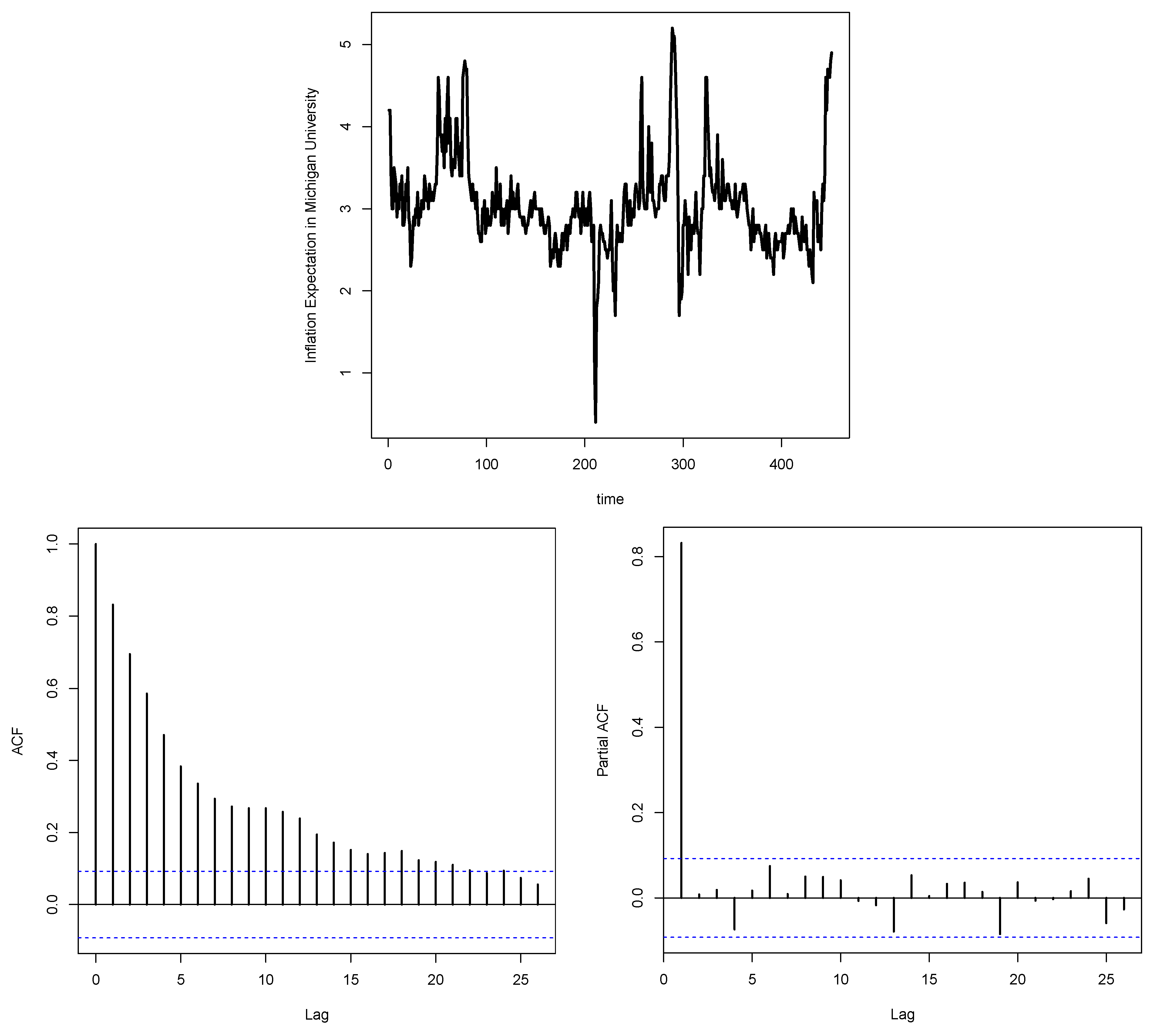
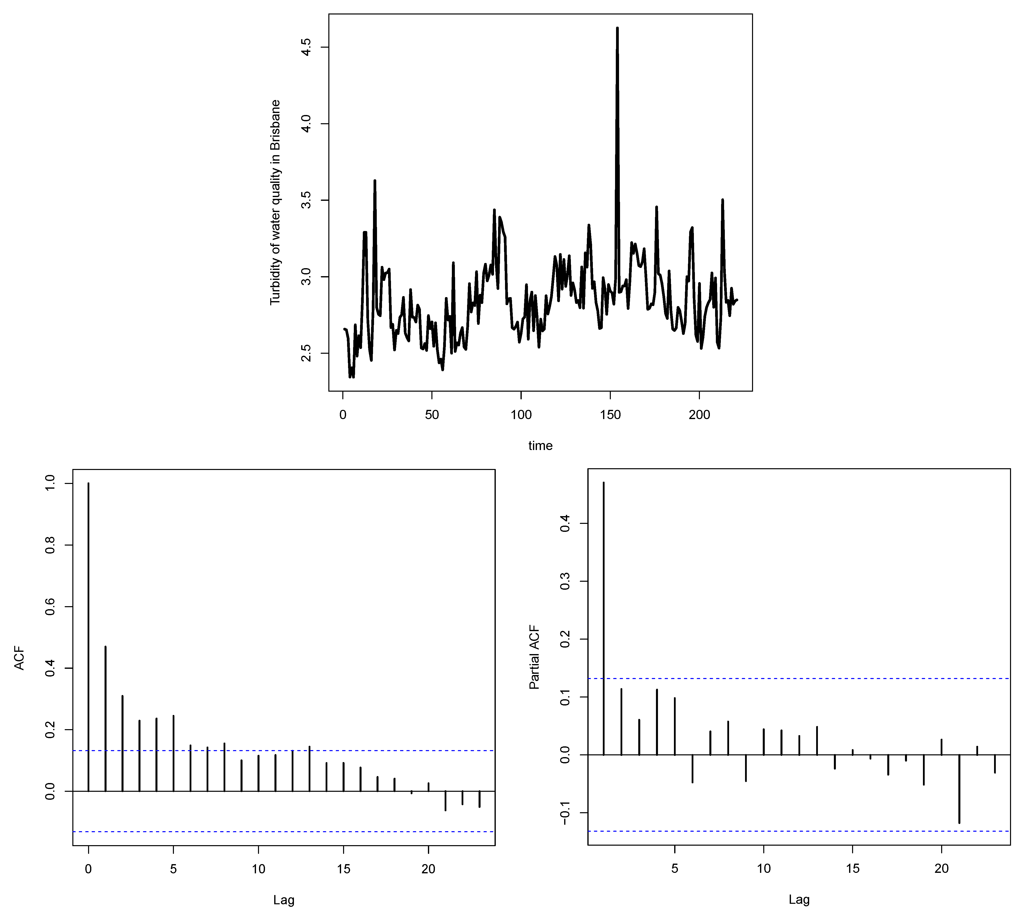
5. Real-Life Data Analysis and Model Selection

In this section, we assess the applicability of the proposed model by utilizing two real-life datasets.

To illustrate and evaluate the performance and competitiveness of the proposed model, we investigated two real-life datasets, outlined as follows:

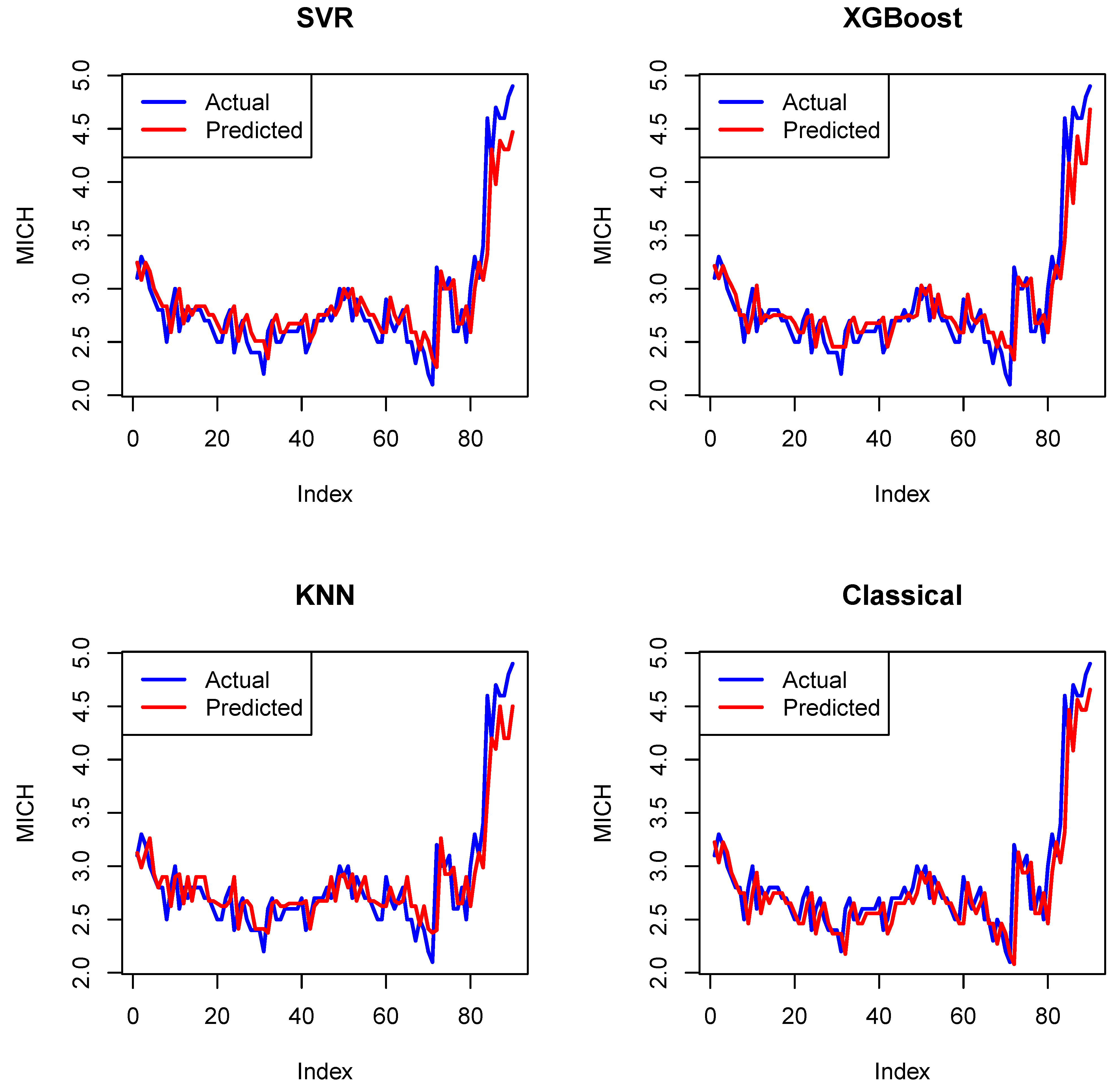
• The first dataset consists of 451 observations, representing the monthly University of Michigan Inflation Expectation (MICH) from 5 January 1984 to 1 November 2021. These data can be found at https://fred.stlouisfed.org/series/MICH (accessed on 12 June 2024).
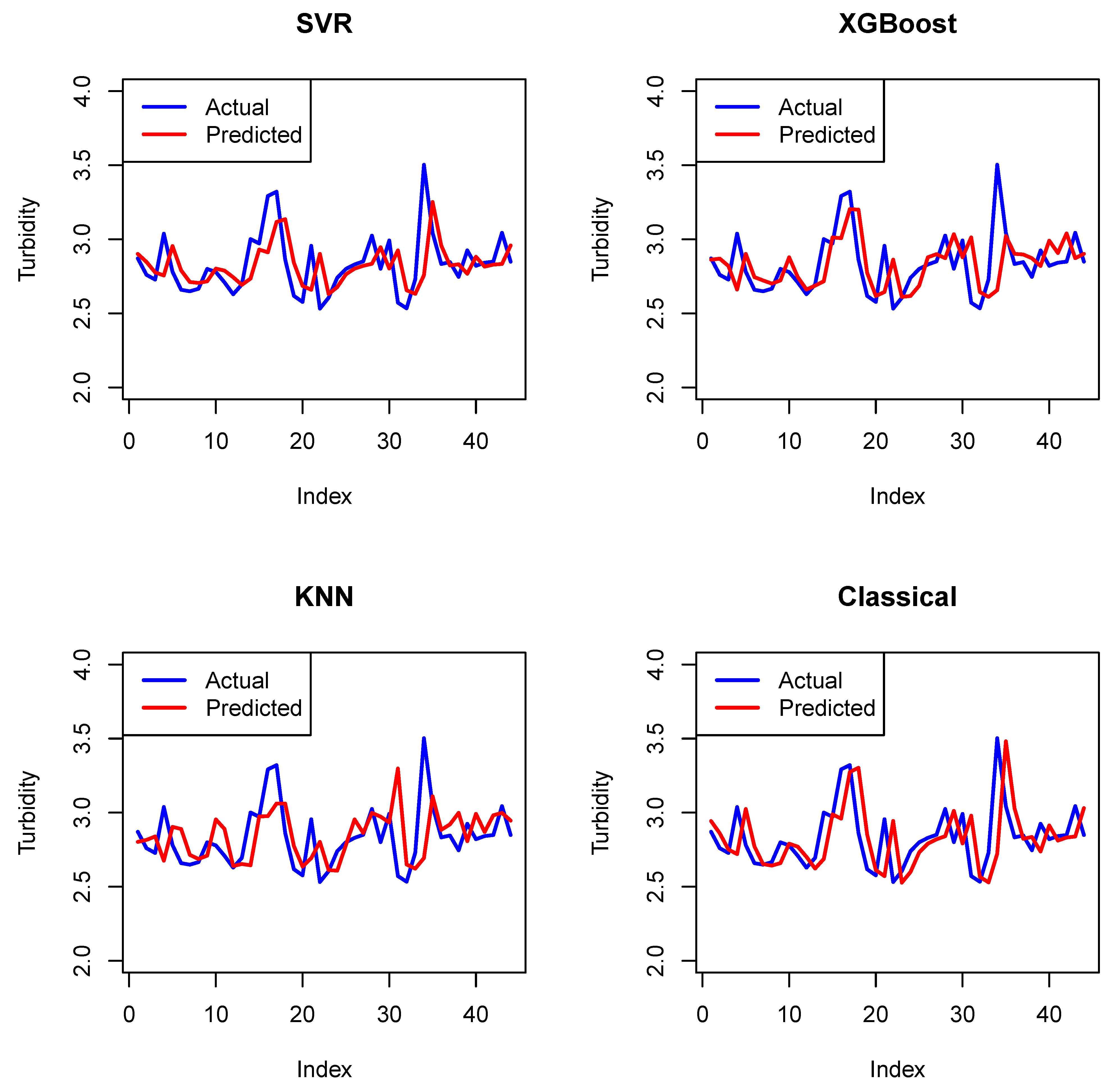
• The second dataset comprises 221 observations that represent the turbidity of water quality in Brisbane, measured every 10 min during the period from 23 June 2024, at 07:10, to 24 June 2024, at 19:30. These data can be obtained from https://www.kaggle.com/datasets/downshift/water-quality-monitoring-dataset (accessed on 3 October 2024).

The time series, autocorrelation (ACF), and partial autocorrelation (PACF) functions for the two datasets are displayed in Figure 4 and Figure 5, respectively. Based on these plots, we can conclude that the PACF cuts off after lag one, indicating that the datasets are appropriate for an AR(1) model. Additionally, the ACF dies down rapidly. These two figures suggest that the two datasets are stationary. We further validate this conclusion through a stationarity test as follows.

Figure 4. The time series, ACF, and PACF plots of monthly University of Michigan Inflation Expectation (MICH).

Figure 5. The time series, ACF, and PACF plots of the turbidity of water quality in Brisbane.

The augmented Dickey–Fuller (ADF) test is a statistical tool used to determine whether a time series is stationary or not. If the p-value from the test is less than the designated significance level (0.05), we reject the null hypothesis of non-stationarity, indicating that the time series is stationary. The ADF test was applied using the adf.test function from the tseries package in R. According to the p-values shown for each dataset in Table 3, we can conclude that the datasets are stationary.

Table 3. Descriptive statistics of University of Michigan Inflation Expectation and Brisbane water quality datasets.

Dataset	n	Min.	${\mathit{Q}}_1$	${\mathit{Q}}_2$	Mean	${\mathit{Q}}_3$	Max.	Var	p-Value (ADF)
MCIH	451	0.400	2.700	3.000	3.044	3.200	5.200	0.3385	0.03571
Turbidity	221	2.344	2.667	2.821	2.843	2.981	4.625	0.0665	0.01031

To compare the proposed process, SBL-AR(1), we will utilize the earlier two datasets alongside the following relevant non-Gaussian AR(1) models associated with their Gaussian log-likelihood functions.

• E-AR(1) with exponential marginals (Gaver and Lewis [1]):

  $$\begin{array}{ccc}\hfill l(\rho ,\lambda ,\beta )& =& {\displaystyle \frac{-n}{2}}log\left(2\pi \right)\hfill \\ & -& {\displaystyle \frac{1}{2}}{\displaystyle \sum _{t=2}^n}\left\{log\left({\displaystyle \frac{1-{\rho }^2}{{\lambda }^2}}\right)+{\displaystyle \frac{{\lambda }^2}{1-{\rho }^2}}{\left(x_t-\rho x_{t-1}-{\displaystyle \frac{1-\rho }{\lambda }}\right)}^2\right\}.\hfill \end{array}$$
• G-AR(1) with gamma marginals (Gaver and Lewis [1]):

  $$\begin{array}{ccc}\hfill l(\rho ,\lambda ,k)& =& {\displaystyle \frac{-n}{2}}log\left(2\pi \right)\hfill \\ & -& {\displaystyle \frac{1}{2}}{\displaystyle \sum _{t=2}^n}\left\{log{\displaystyle \frac{k\left(1-{\rho }^2\right)}{{\lambda }^2}}+{\displaystyle \frac{{\lambda }^2}{k\left(1-{\rho }^2\right)}}{\left(x_t-\rho x_{t-1}-{\displaystyle \frac{k(1-\rho )}{\lambda }}\right)}^2\right\}.\hfill \end{array}$$
• INGAR(1)-I with inverse Gaussian marginals (Abraham and Balakrishna [4]):

  $$\begin{array}{ccc}\hfill l(\rho ,\lambda ,\mu )& =& {\displaystyle \frac{-n}{2}}log\left(2\pi \right)\hfill \\ & -& {\displaystyle \frac{1}{2}}{\displaystyle \sum _{t=2}^n}\left\{log\left(1-{\rho }^2\right)\mu +{\displaystyle \frac{1}{(1-{\rho }^2)\mu }}{(x_t-\rho x_{t-1}-(1-\rho )\mu )}^2\right\}.\hfill \end{array}$$
• INGAR(1)-II with inverse Gaussian marginals (Abraham and Balakrishna [4]):

  $$\begin{array}{ccc}\hfill l(\rho ,\lambda ,\mu )& =& {\displaystyle \frac{-n}{2}}log\left(2\pi \right)\hfill \\ & -& {\displaystyle \frac{1}{2}}{\displaystyle \sum _{t=2}^n}\left\{log\left(1-{\rho }^2\right){\displaystyle \frac{{\mu }^3}{\lambda }}+{\displaystyle \frac{\lambda }{(1-{\rho }^2){\mu }^3}}{(x_t-\rho x_{t-1}-(1-\rho )\mu )}^2\right\}.\hfill \end{array}$$
• L-AR(1) with Lindley marginals (Bakouch and Popovíc [7]):

  $$\begin{array}{ccc}\hfill l(\rho ,\lambda )& =& {\displaystyle \frac{-n}{2}}log\left(2\pi \right)-{\displaystyle \frac{1}{2}}{\displaystyle \sum _{t=2}^n}\left\{log{\displaystyle \frac{(1-{\rho }^2)\left({\lambda }^2+4\lambda +2\right)}{{\lambda }^2{(1+\lambda )}^2}}\right.\hfill \\ & +& \left.{\displaystyle \frac{{\lambda }^2{(1+\lambda )}^2}{(1-{\rho }^2)\left({\lambda }^2+4\lambda +2\right)}}{\left(x_t-\rho x_{t-1}-(1-\rho ){\displaystyle \frac{(\lambda +2)}{\lambda (1+\lambda )}}\right)}^2\right\}.\hfill \end{array}$$
• GaL-AR(1) with gamma Lindley marginals (Mello et al. [9]):

  $$\begin{array}{ccc}\hfill l(\rho ,\lambda ,\beta )& =& {\displaystyle \frac{-n}{2}}log\left(2\pi \right)\hfill \\ & -& {\displaystyle \frac{1}{2}}{\displaystyle \sum _{t=2}^n}\left\{log{\displaystyle \frac{(-{(-2\beta \lambda +\lambda )}^2+2{\beta }^2(1+3\lambda )-2\beta (\beta \lambda -3\beta {\lambda }^2+2{\lambda }^2))(1-{\rho }^2)}{{\lambda }^2{\beta }^2{(1+\lambda )}^2}}\right.\hfill \\ & +& {\displaystyle \frac{{\lambda }^2{\beta }^2{(1+\lambda )}^2}{(-{(-2\beta \lambda +\lambda )}^2+2{\beta }^2(1+3\lambda )-2\beta (\beta \lambda -3\beta {\lambda }^2+2{\lambda }^2))(1-{\rho }^2)}}\hfill \\ & \times & \left.{\left(x_t-\rho x_{t-1}-(1-\rho ){\displaystyle \frac{2\beta (1+\lambda )-\lambda }{\lambda \beta (1+\lambda )}}\right)}^2\right\}.\hfill \end{array}$$
• AR-L(1) with Lindley innovations (Nitha and Krishnarani [21]):

  $$\begin{array}{ccc}\hfill l(\rho ,\lambda )& =& {\displaystyle \frac{-n}{2}}log\left(2\pi \right)-{\displaystyle \frac{1}{2}}{\displaystyle \sum _{t=2}^n}\left\{log{\displaystyle \frac{\left({\lambda }^2+4\lambda +2\right)}{{\lambda }^2{(1+\lambda )}^2(1-{\rho }^2)}}\right.\hfill \\ & +& \left.{\displaystyle \frac{{\lambda }^2{(1+\lambda )}^2(1-{\rho }^2)}{\left({\lambda }^2+4\lambda +2\right)}}{\left(x_t-\rho x_{t-1}-{\displaystyle \frac{(\lambda +2)}{\lambda (1+\lambda )}}\right)}^2\right\}.\hfill \end{array}$$

The GE method was used to estimate the unknown parameters for all the considered models. Numerical methods were applied to determine these parameter values, utilizing the optim function in R along with the conjugate gradients (CG) method for this purpose. For each dataset and model, the Gaussian likelihood estimates, the Akaike information criterion (AIC), Bayesian information criterion (BIC), and Hannan–Quinn information criterion (HQIC) were computed. We evaluated model performance using information criteria statistics. The model that performs best is the one with the smallest values for these statistics. The results of the goodness-of-fit statistics and the GE estimates, including their standard errors (SE), are summarized in Table 4 and Table 5. From these tables, it is evident that the SBL-AR(1) model achieved the smallest values for AIC, BIC, and HQIC. Consequently, we can conclude that the proposed model performed well for both datasets; hence, the SBL-AR(1) model provides the best fit among the AR(1) models considered.

Table 4. Estimated parameters, AIC, BIC, and HQIC for monthly University of Michigan Inflation Expectation dataset.

Model	GE Estimates (SE)	AIC	BIC	HQIC
SBL-AR	$\widehat{\rho }$ = 0.9722689 (0.006470897) $\widehat{\theta }$ = 1.2350076 (0.137368908)	253.3235	261.5464	256.5642
L-AR	$\widehat{\rho }$ = 0.9615126 (0.00501119) $\widehat{\lambda }$ = 1.1524668 (0.06931619)	268.7283	276.9512	271.9689
GaL-AR	$\widehat{\rho }$ = 0.9695075 (0.005533153) $\widehat{\lambda }$ = 1.0218001 (0.108046443) $\widehat{\beta }$ = 0.9895284 (0.293700792)	262.2251	274.5595	267.0861
E-AR	$\widehat{\rho }$ = 0.9597630 (0.00505366) $\widehat{\lambda }$ = 0.8991799 (0.05621214)	274.4090	282.6319	277.6497
G-AR	$\widehat{\rho }$ = 0.9736072 (0.007168259) $\widehat{\lambda }$ = 0.5314403 (0.203203788) $\widehat{k}$ = 0.5480252 (0.297268206)	265.7606	278.0950	270.6216
INGAR-I	$\widehat{\rho }$ = 0.9582729 (0.003857915) $\widehat{\mu }$ = 1.1860471 (0.096928851)	274.3043	282.5272	277.5449
INGAR-II	$\widehat{\rho }$ = 0.9932729 (0.00163749) $\widehat{\mu }$ = 1.9887342 (0.44900524) $\widehat{\lambda }$ = 1.0075656 (0.58975847)	260.5591	272.8935	265.4201
AR-L	$\widehat{\rho }$ = 0.9353976 (0.006316815) $\widehat{\theta }$ = 8.6482145 (0.540094410)	270.5227	278.7457	273.7634

Table 5. Estimated parameters, AIC, BIC, and HQIC for Brisbane water quality dataset.

Model	GE Estimates (SE)	AIC	BIC	HQIC
SBL-AR	$\widehat{\rho }$ = 0.9677021 (0.00751236) $\widehat{\theta }$ = 1.6010980 (0.17560826)	46.89545	53.69178	49.63968
L-AR	$\widehat{\rho }$ = 0.9717271 (0.006628198) $\widehat{\lambda }$ = 1.1756744 (0.127043976)	49.18248	55.97881	51.92672
GaL-AR	$\widehat{\rho }$ = 0.9718353 (0.006936761) $\widehat{\lambda }$ = 1.1164845 (0.175881692) $\widehat{\beta }$ = 0.7821798 (0.246680549)	51.60417	61.79866	55.72052
E-AR	$\widehat{\rho }$ = 0.9633879 (0.006277054) $\widehat{\lambda }$ = 1.0429649 (0.090100243)	56.95756	63.75388	59.70179
G-AR	$\widehat{\rho }$ = 0.9524641 (0.008869184) $\widehat{\lambda }$ = 1.5172295 (0.395848932) $\widehat{k}$ = 1.4776463 (0.495027829)	71.70304	81.89753	75.81939
INGAR-I	$\widehat{\rho }$ = 0.9622654 (0.004742255) $\widehat{\mu }$ = 0.8843855 (0.098468366)	59.35630	66.15262	62.10053
INGAR-II	$\widehat{\rho }$ = 0.9970946 (0.0002890516) $\widehat{\mu }$ = 1.5959593 (0.2560154481) $\widehat{\lambda }$ = 0.3071916 (0.1316577834)	50.63486	60.82935	54.75122
AR-L	$\widehat{\rho }$ = 0.9049345 (0.00977161) $\widehat{\theta }$ = 7.0817431 (0.56402558)	96.52965	103.32598	99.27389

For each dataset, the residuals, $a_t$, were computed from the fitted model, given by Equation (2), using the estimated parameter $\widehat{\rho }$ in Table 4 and Table 5. To assess the presence of autocorrelation in these residuals, both the Box–Pierce and Ljung–Box tests were performed. The results, summarized in Table 6, indicate that for all cases, the p-values exceeded 0.05, indicating no significant autocorrelation in the residuals of the fitted model.

Table 6. Ljung–Box and Box–Pierce test results for residual autocorrelation.

Dataset	p-Value of Ljung-Box Test	p-Value of Box-Pierce Test
MCIH	0.6371	0.6382
Turbidity	0.3715	0.3747

6. Forecasting

Forecasting time series data is essential for predicting future trends in non-Gaussian contexts, where traditional Gaussian models may fail to capture skewed or fat-tailed data distribution. The proposed SBL-AR(1) model utilizes size-biased Lindley marginals and employs both classical conditional expectation method and machine learning techniques, demonstrating a superior accuracy in predicting the considered real-world datasets.

6.1. Classical Conditional Expectation Method

This classical method is one of the most widely used forecasting methods relies on conditional expectations. The forecast ${\widehat{X}}_{t+k}$ is essentially the expected value of $X_{t+k}$ given all the available information up to time t. The one- and k-step-ahead forecasts for $X_{t+1}$ and $X_{t+k}$, respectively, are concluded by Equation (23) as follows:

$$\begin{array}{c}\hfill {\widehat{X}}_{t+1}=E\left(X_{t+1}\right|X_t=x_t)=\rho x_t+(1-\rho ){\displaystyle \frac{2(\theta +3)}{\theta (\theta +2)}},\end{array}$$

and

$$\begin{array}{c}\hfill {\widehat{X}}_{t+k}=E\left(X_{t+k}\right|X_t=x_t)={\rho }^k{x}_t+(1-{\rho }^k){\displaystyle \frac{2(\theta +3)}{\theta (\theta +2)}}.\end{array}$$

The parameters $\rho$ and $\theta$ are replaced with their GE estimates. Then

$$\begin{array}{c}\hfill {\widehat{X}}_{t+1}=E\left(X_{t+1}\right|X_t=x_t)=\widehat{\rho }{x}_t+(1-\widehat{\rho }){\displaystyle \frac{2(\widehat{\theta }+3)}{\widehat{\theta }(\widehat{\theta }+2)}},\end{array}$$

and

$$\begin{array}{c}\hfill {\widehat{X}}_{t+k}=E\left(X_{t+k}\right|X_t=x_t)={\widehat{\rho }}^k{x}_t+(1-{\widehat{\rho }}^k){\displaystyle \frac{2(\widehat{\theta }+3)}{\widehat{\theta }(\widehat{\theta }+2)}}.\end{array}$$

6.2. Machine Learning Forecasting Methods

Unlike classical statistical methods, which rely on predefined theoretical assumptions, machine learning (ML) approaches are non-parametric and data-driven, learning patterns directly from observed data to adapt flexibly to complex structures. These methods typically involve training algorithms on historical data to learn underlying relationships, which can then be used to make predictions about future values. To model the autoregressive behavior of the time series using ML methods, we adopted an AR(1) structure where the current observation $x_t$ is predicted using its immediate lag, $x_{t-1}$. The data were first transformed into a supervised learning format by creating a lag-1 feature. The dataset was then divided into training and testing sets (e.g., 80% and 20%, respectively). In the following subsections, we examine the use of some machine learning (ML) methods, which are support vector regression, k-nearest neighbors, and extreme gradient boosting, to forecast data generated by AR(1) processes.

6.2.1. Support Vector Regression

Support vector regression (SVR) is used to model both linear and nonlinear relationships in time series data, adept in complex scenarios while remaining applicable to simpler linear cases like the autoregressive (AR(1)) process. It finds a function predicting targets accurately within a small error margin ($ϵ$) (Smola and Schölkopf [22]), effective for time series forecasting.

Given a training set $\{(x_1,y_1),...,(x_N,y_N)\}$, where $x_i$ represents the input features (e.g., lagged time series values) and $y_i$ denotes the corresponding target values, the goal is to find a linear function $f\left(x\right)=w^{T}x+b$ that minimizes the cost function:

$$\begin{array}{c}\hfill \underset{w,b,\xi ,{\xi }^{\ast }}{min}\left\{{\displaystyle \frac{1}{2}}{∥w∥}^2+C{\displaystyle \sum _{i=1}^n}\left({\xi }_i+{\displaystyle {\xi }_i^{\ast }}\right)\right\}\\ \hfill \mathrm{subject}\mathrm{to}\left\{\begin{array}{c}{y}_i-(w^T{x}_i+b)\le ϵ+{\xi }_i,\hfill \\ (w^T{x}_i+b)-y_i\le ϵ+{\displaystyle {\xi }_i^{\ast }},\hfill \\ {\xi }_i,{\displaystyle {\xi }_i^{\ast }}\ge 0\hfill \end{array}\right.\end{array}$$

where w is the weight vector, b is the bias term, ${\xi }_i$ and ${\displaystyle {\xi }_i^{\ast }}$ are slack variables allowing deviations beyond $ϵ$, and C controls the trade-off between model complexity and training error.

We employed the svm function from the e1071 package in R (version 4.4.3), specifying a linear kernel and epsilon-insensitive loss (type = “eps-regression”), which aligns with the assumptions of the AR(1) model.

6.2.2. Extreme Gradient Boosting

Extreme gradient boosting (XGBoost) is based on gradient-boosted decision trees, optimized for speed and performance (Chen and Guestrin [23]). XGBoost constructs its model by building decision trees sequentially, where each new tree is trained to correct the errors made by the previous ones. This process is guided by an objective function that balances the accuracy and complexity of the model. The objective function minimized during training combines a loss term measuring prediction errors (e.g., squared error) and a regularization term penalizing complexity to prevent overfitting, expressed as

$$\mathrm{Obj}\left(\theta \right)={\displaystyle \sum _{i=1}^n}{(y_i-{\widehat{y}}_i)}^2+{\displaystyle \sum _{k=1}^K}\Omega \left(f_k\right),$$

where $f_k$ represents each regression tree, and $\Omega \left(f_k\right)$ is a regularization function controlling the complexity of each tree.

The XGBoost algorithm was implemented in R using the xgboost package, with data formatted as a matrix or xgb.DMatrix for optimized performance and trained via xgb.train using the “reg:squarederror” objective function.

6.2.3. K-Nearest Neighbors

The K-nearest neighbors (KNN) algorithm predicts outcomes by measuring distances (e.g., $d(x,x_i)=|x-x_i|$) between a new data point and training samples, selecting the K closest neighbors. The final prediction is the average of these neighbors’ target values:

$$\widehat{y}={\displaystyle \frac{1}{K}}{\displaystyle \sum _{j=1}^K}{y}_{\left(j\right)},$$

where $y_{\left(j\right)}$ denotes the $j^{th}$ neighbor’s value (Kramer, O. [24]).

We used the FNN package in R to apply the KNN method. The knn.reg function was used to make predictions based on the average of the closest points in the data.

6.3. Forecasting Evaluation

To assess the performance of the forecasting model, several commonly used error metrics were employed to quantify the accuracy of the predictions. Below are the most commonly used measures:

• Root Mean Squared Error (RMSE)
  It is the square root of MSE; in the same units as the target variable:

  $$\mathrm{RMSE}=\sqrt{{\displaystyle \frac{1}{n}}{\displaystyle \sum _{t=1}^n}{(y_t-{\widehat{y}}_t)}^2}.$$
• Mean Absolute Error (MAE)
  It measures the average absolute difference between predicted and actual values:

  $$\mathrm{MAE}={\displaystyle \frac{1}{n}}{\displaystyle \sum _{t=1}^n}|y_t-{\widehat{y}}_t|.$$
• Mean Absolute Percentage Error (MAPE)
  It measures error as a percentage of actual values:

  $$\mathrm{MAPE}={\displaystyle \frac{1}{n}}{\displaystyle \sum _{t=1}^n}\left|{\displaystyle \frac{y_t-{\widehat{y}}_t}{y_t}}\right|\times 100\%.$$

• For the considered machine learning methods, hyperparameter tuning was performed via grid search to determine the optimal values for the key parameters that achieve the lowest RMSE of each method.

Table 7 and Table 8 evaluate the one-step-ahead forecasting performance of classical (SBL-AR(1) conditional expectation) and machine learning methods. While XGBoost achieved the lowest errors for the MICH dataset in MAE and MAPE and SVR excelled for the Turbidity dataset, the classical method demonstrated notable competitiveness. For the MICH dataset, the classical method outperformed SVR in all measures and outperformed KNN in MAE (0.1809712 vs. 0.1831944) and MAPE (6.098343 vs. 6.270608); it also closely matched XGBoost. For the Turbidity dataset, although the machine learning methods are superior, the values of the classical method are still close to the KNN method. These results highlight the competitiveness of the classical forecasting method under the SBL-AR(1) model against modern machine learning techniques due to its parametric structure, which effectively captures skewed and fat-tailed data, avoiding overfitting (that is, the predicted values match the true observed values). These results also underscore that while ML methods adapt flexibly to data patterns, the classical approach based on the structure of SBL-AR(1) retains predictive power, particularly in scenarios where parametric assumptions align well with the data’s inherent dynamics.

Table 7. Model performance measures for forecasting MICH dataset values.

Measure	RMSE	MAE	MAPE
SVR	0.2695047	0.1890921	6.447078%
XGBoost	0.2621252	0.1792437	6.073617%
KNN	0.2508839	0.1831944	6.270608%
Classical	0.2679958	0.1809712	6.098343%

Table 8. Model performance measures for forecasting Turbidity dataset values.

Measure	RMSE	MAE	MAPE
SVR	0.1993664	0.1448703	4.984548%
XGBoost	0.2093979	0.1462492	5.040056%
KNN	0.2249225	0.1538455	5.342222%
Classical	0.2300879	0.1660202	5.728669%

Actual and predicted values for each dataset using all of the forecasting methods are shown in Figure 6 and Figure 7. The classical SBL-AR(1) method’s predictions in these figures closely follow the actual data trends, showing smoother alignment compared to the machine learning methods. This strong fit arises because the SBL-AR(1) model is specifically designed for the data’s skewed and positive-valued nature, utilizing its parametric structure. While some ML methods achieved slightly lower errors in Table 7 and Table 8, the figures confirm the classical method’s capability in capturing the data’s inherent patterns without overfitting.

Figure 6. Actual and predicted values of University of Michigan Inflation Expectation.

Figure 7. Actual and predicted values of turbidity of water quality in Brisbane.

7. Conclusions

In this study, we introduced a first-order autoregressive process based on the size-biased Lindley distribution (SBL-AR(1)) model. We explored several theoretical properties of the process, including its innovation distribution, Laplace transform, conditional mean and variance, autocorrelation structure, and spectral density. To estimate the model parameters, we employed both conditional least squares and Gaussian estimation methods.

A comprehensive Monte Carlo simulation was conducted to evaluate the behavior of the estimators, demonstrating their efficiency. Furthermore, the applicability of the SBL-AR(1) model was illustrated using two real-world datasets. In both cases, the model provided a superior fit compared to several alternative non-Gaussian AR(1) processes, as evidenced by goodness-of-fit statistics. In addition, both classical statistical method and machine learning techniques were used for forecasting. The classical method has demonstrated strong competitiveness when compared to machine learning methods.

Future work may consider extending the model to higher-order autoregressive structures.

References

- Gaver, D.P.; Lewis, P.A. First-order autoregressive gamma sequences and point processes. Adv. Appl. Probab. 1980, 12, 727–745. [Google Scholar] [CrossRef]
- Sim, C.H. Simulation of Weibull and gamma autoregressive stationary process. Commun. Stat. Simul. Comput. 1986, 15, 1141–1146. [Google Scholar] [CrossRef]
- Mališić, J.D. Mathematical Statistics and Probability Theory: Volume B; Springer: Berlin/Heidelberg, Germany, 1987. [Google Scholar]
- Abraham, B.; Balakrishna, N. Inverse Gaussian autoregressive models. J. Time Ser. Anal. 1999, 20, 605–618. [Google Scholar] [CrossRef]
- Jose, K.K.; Tomy, L.; Sreekumar, J. Autoregressive processes with normal-Laplace marginals. Stat. Probab. Lett. 2008, 78, 2456–2462. [Google Scholar] [CrossRef]
- Popović, B.V. AR (1) time series with approximated beta marginal. Publ. Inst. Math. 2010, 88, 87–98. [Google Scholar] [CrossRef]
- Bakouch, H.S.; Popović, B.V. Lindley first-order autoregressive model with applications. Commun. Stat. Theory Methods 2016, 45, 4988–5006. [Google Scholar] [CrossRef]
- Nitha, K.U.; Krishnarani, S.D. On a class of time series model with double Lindley distribution as marginals. Statistica 2021, 81, 365–382. [Google Scholar]
- Mello, A.B.; Lima, M.C.; Nascimento, A.D. The title of the cited article. Environmetrics 2022, 33, e2724. [Google Scholar] [CrossRef]
- Jilesh, V.; Jayakumar, K. On first order autoregressive asymmetric logistic process. J. Indian Soc. Probab. Stat. 2023, 24, 93–110. [Google Scholar] [CrossRef]
- Nitha, K.U.; Krishnarani, S.D. Exponential-Gaussian distribution and associated time series models. Revstat Stat. J. 2023, 21, 557–572. [Google Scholar]
- Patil, G.P.; Rao, C.R. Weighted distributions and size-biased sampling with applications to wildlife populations and human families. Biometrics 1978, 34, 179–189. [Google Scholar] [CrossRef]
- Scheaffer, R. Size-biased sampling. Technometrics 1972, 14, 635–644. [Google Scholar] [CrossRef]
- Singh, S.K.; Maddala, G.S. Modeling Income Distributions and Lorenz Curves; Springer: Berlin/Heidelberg, Germany, 2008. [Google Scholar]
- Drummer, T.D.; McDonald, L.L. Size bias in line transect sampling. Biometrics 1987, 43, 13–21. [Google Scholar] [CrossRef]
- Ayesha, A. Size biased Lindley distribution and its properties a special case of weighted distribution. J. Appl. Math. 2017, 8, 808–819. [Google Scholar] [CrossRef]
- Whittle, P. Gaussian estimation in stationary time series. Bull. Int. Stat. Inst. 1961, 39, 105–129. [Google Scholar]
- Crowder, M. Gaussian estimation for correlated binomial data. J. R. Stat. Soc. Ser. B (Stat. Methodol.) 1985, 47, 229–237. [Google Scholar] [CrossRef]
- Al-Nachawati, H.; Alwasel, I.; Alzaid, A.A. Estimating the parameters of the generalized Poisson AR (1) process. J. Stat. Comput. Simul. 1997, 56, 337–352. [Google Scholar] [CrossRef]
- Alwasel, I.; Alzaid, A.; Al-Nachawati, H. Estimating the parameters of the binomial autoregressive process of order one. Appl. Math. Comput. 1998, 95, 193–204. [Google Scholar] [CrossRef]
- Nitha, K.U.; Krishnarani, S.D. On autoregressive processes with Lindley-distributed innovations: Modeling and simulation. Stat. Transit. New Ser. 2024, 25, 31–47. [Google Scholar] [CrossRef]
- Smola, A.J.; Schölkopf, B. A tutorial on support vector regression. Stat. Comput. 2004, 14, 199–222. [Google Scholar] [CrossRef]
- Chen, T.; Guestrin, C. Xgboost: A scalable tree boosting system. In Proceedings of the 22nd ACM SIGKDD International Conference on Knowledge Discovery and Data Mining, San Francisco, CA, USA, 13–17 August 2016; pp. 785–794. [Google Scholar]
- Kramer, O. Dimensionality reduction by unsupervised k-nearest neighbor regression. In Proceedings of the 2011 10th International Conference on Machine Learning and Applications and Workshops, Honolulu, HI, USA, 18–21 December 2011; pp. 275–278. [Google Scholar]
Disclaimer/Publisher’s Note: The statements, opinions and data contained in all publications are solely those of the individual author(s) and contributor(s) and not of MDPI and/or the editor(s). MDPI and/or the editor(s) disclaim responsibility for any injury to people or property resulting from any ideas, methods, instructions or products referred to in the content. |
© 2025 by the authors. Licensee MDPI, Basel, Switzerland. This article is an open access article distributed under the terms and conditions of the Creative Commons Attribution (CC BY) license (https://creativecommons.org/licenses/by/4.0/).