Abstract
Pólya-gamma (PG) augmentation has proven to be highly effective for Bayesian MCMC simulation, particularly for models with binomial likelihoods. This data augmentation strategy offers two key advantages. First, the method circumvents the need for analytic approximations or Metropolis–Hastings algorithms, which leads to simpler and more computationally efficient posterior inference. Second, the approach can be successfully applied to several types of models, including nonlinear mixed-effects models for count data. The effectiveness of PG augmentation has led to its widespread adoption and implementation in statistical software packages, such as version 2.1 of the R package BayesLogit. This success has inspired us to apply this method to the implementation of Section 203 of the Voting Rights Act (VRA), a US law that requires certain jurisdictions to provide non-English voting materials for specific language minority groups (LMGs). In this paper, we show how PG augmentation can be used to fit a Bayesian model that estimates the prevalence of each LMG in each US voting jurisdiction, and that uses a variable selection technique called stochastic search variable selection. We demonstrate that this new model outperforms the previous model used for 2021 VRA data with respect to model diagnostic measures.
Keywords:
small area estimation; Pólya-gamma augmentation; stochastic search variable selection; Bayesian regression; Gibbs sampling; Voting Rights Act MSC:
62F15
1. Introduction
1.1. A Motivating Example
Section 203(b) of the Voting Rights Act (VRA) is an election law that requires some US states or their political subdivisions to make voting materials available in languages other than English. The US Census Bureau determines whether a jurisdiction, e.g., county, is subject to such requirements based on the rates of limited English language proficiency and illiteracy within designated population subgroups, called language minority groups (LMGs), in that jurisdiction. For the purposes of VRA coverage determinations, limited English proficiency (LEP) is defined as speaking a language other than English at home, and speaking English less than “Very Well”. Illiteracy (ILL) is defined as having less than a 5th-grade education. A more detailed discussion of the legal and statistical criteria used to make VRA coverage determinations is available in Slud et al. [1].
To make these determinations, the Census Bureau must estimate the number of voting-age (18 or over) people (VOT), voting-age citizens (CIT), voting-age citizens who have limited English proficiency (LEP), and voting-age citizens with limited English proficiency who are illiterate (ILL) in each of these geographies. The Census Bureau initially used “direct” estimates based on data from the long-form of the Decennial Census (later replaced by the American Community Survey, or ACS) to approximate these quantities. The term “direct” indicates that an estimate does not use any statistical model or auxiliary information beyond the survey weights and observations within that area. However, since 2011, Section 203 determinations have been based on estimates from small-area models. These statistical models were updated in 2014 by Joyce et al. [2], who developed a Bayesian hierarchical model, and Slud et al. [3], who adopted a Dirichlet-multinomial model.
In the VRA 2021 determinations, model-based estimates were obtained using both frequentist and Bayesian methods [1]. The frequentist method used adaptive Gaussian quadrature [4] to fit random effects models for LMGs with a sample in less than 700 jurisdictions (counties and MCDs), or less than 3000 jurisdictions where most citizens did not have severe illiteracy. The Bayesian model was fitted using STAN [5], which only worked well for large LMGs. Models fit with STAN had relatively slow and unstable convergence in smaller LMGs even when using priors recommended for computational efficiency, such as the LKJ prior for the random-effects covariance distribution. In addition, both methods used covariates that were selected based on their performance in a few large LMGs to model all LMGs, rather than performing independent variable selection procedures in the models for smaller groups. More details on the VRA 2021 methods are described in Slud et al. [1].
Table 1 shows a dataset that contains hypothetical examples of jurisdiction-level estimates that VRA models might produce for an LMG. For this LMG, let , , , and represent VOT, CIT, LEP, and ILL, respectively, in jurisdiction j. Then, in Table 1, CITprop, LEPprop, and ILLprop represent the direct estimates of the ratios , , and , respectively. The model-based predictions of these ratios are represented by , , and , respectively.

Table 1.
Hypothetical VRA proportions for an LMG.
Note that the model-based estimates are similar to the direct estimates for jurisdiction 1, which has a large number of voting-age residents. However, these estimates differ in jurisdictions with fewer voting-age persons. This pattern occurs because direct estimates perform well in large samples, but poorly when sample sizes are small. Model-based estimates use vectors of auxiliary covariates, denoted in Table 1 by X, to help improve their low sample performance.
The new model introduced in this article uses Pólya-gamma (PG) augmentation [6] to estimate Bayesian models for all LMGs and jurisdictions. This enables the new model to more easily implement stochastic search variable selection (SSVS) within each LMG to select covariates, which allows our new model to outperform the older models in terms of diagnostic metrics.
1.2. Utility of Pólya-Gamma Augmentation in Bayesian Methods
Pólya-gamma (PG) augmentation, as introduced by Polson et al. [6], is an efficient method for Bayesian inference in models with binomial likelihoods. The application of PG augmentation yields closed-form expressions for full conditionals of posterior distributions in sampling algorithms like Markov chain Monte Carlo (MCMC), which eliminates the need for analytic approximations, numerical integration, or Metropolis–Hastings algorithms. This allows the construction of simple and effective Gibbs samplers for models with binomial likelihoods, particularly logistic regression. The method has been successfully applied to various models, including logistic regression and nonlinear mixed-effects models [6]. In practice, the PG Gibbs sampler for Bayesian logistic regression involves two main steps in each iteration: sampling PG random variables and drawing from a multivariate normal distribution. This approach has been implemented in various statistical software packages, such as Version 2.1 of the R package BayesLogit [7].
The remainder of this paper is organized into the following sections. Section 2 reviews the 2021 VRA model, introduces PG augmentation, and explains a basic application in the context of the VRA data. Section 3 builds on this foundation to introduce the new Bayesian multinomial logit model, and describes a Gibbs sampling algorithm that makes use of PG augmentation to fit it. Section 4 applies the new model to the data used for the 2021 VRA determinations and shows its superior diagnostic results compared with the 2021 model results. Finally, Section 5 discusses the results.
2. The Pólya-Gamma Distribution for Binomial VRA Datasets
2.1. The 2021 VRA Model
The 2021 VRA model was constructed by modeling the counts mentioned in Section 1 using a multinomial distribution. Specifically, for each jurisdiction j where , and is the number of voting-age people in j, we model
where , , , and are - , - , - , and , respectively.
An equivalent formulation of this model treats the M variables in Equation (1) as the composition of three conditionally binomial () models:
The intuition behind the success probabilities in these distributions is as follows. In the multinomial model, represents the marginal probability that a voting-age person is not a citizen. Thus, if we ignore the other categories, can be modeled as a binomial distribution counting the number of voting-age non-citizens against the number of voting-age citizens. Similarly, the marginal probability that a person is a voting-age citizen and is not LEP is in the multinomial model. It can be inferred that is the marginal probability that a voting-age person is a citizen. Thus, the probability of a voting-age person not having limited English proficiency conditional on being a citizen is . By the same logic, the marginal probability that a voting-age person is a citizen and LEP but not ILL is in the multinomial model, and the marginal probability that a voting-age person is a citizen and is LEP is . Thus, the conditional probability of a voting-age person not being ILL given that they are a citizen and have LEP is . is known given , and , and thus does not need to be modeled.
The complements of the “success” probabilities of the binomial distributions for , , and can be interpreted as estimates of the ratios , , and in jurisdiction j. With this notation, the probabilities in Equation (1) can be written for each jurisdiction j as
This means that we can model the multinomial success probabilities in (1) by modeling the binomial success probabilities in (2), and we can model the binomial success probabilities in (2) by modeling the ratios. To model the ratios, we assume that
where
and the u are multivariate normal random variables with a zero mean and variance parameter
This specification is called the “multinomial logit normal” (MLN) model due to the multinomial outcome described in Equation (1), the logistic link function in Equation (3), and the multivariate normal random effects. When these parameters are estimated, we can use them to derive model-based estimates of , , and similar to the hypothetical examples in Table 1. Specifically, for jurisdiction j, we estimate as , as , and as . The difficulty of estimating these parameters stems from the nonlinearity of the logistic link function in Equation (3). The Pólya-gamma augmentation makes the estimation process linear, resulting in closed-form solutions for the posterior distributions of our parameters.
2.2. The Pólya-Gamma (PG) Distribution
A PG random variable is defined as an infinite weighted sum of gamma random variables. Specifically, if , where b > 0 and c∈, then:
where denotes equality in distribution, and are independent gamma random variables. Polson et al. [6] proved the following useful property of the PG variable. Let denote a constant, e.g., a linear combination of covariates X and their coefficients . Then, the following equation holds for an exponential functional form:
where and . The utility of the above equation is that for , we can express the contribution of jurisdiction j to the likelihood as
where Note that if we condition on , the kernel of the posterior distribution for looks similar to a Gaussian density function:
where . Step (8) is justified because conditional on , the expectation in (6) is constant. Step (9) is derived by completing the square. From this, Step (10) can be derived using algebra.
In summary, if our prior on is Gaussian (quadratic in ), then (7) has a closed-form solution. This enables us to construct a Gibbs sampler for , by repeatedly sampling and then sampling .
2.3. A Simplified Application of Pólya-Gamma Augmentation
To illustrate the application of PG augmentation to the 2021 VRA model, consider jurisdiction j, for , where N denotes the total number of jurisdictions. Let denote the number of voting-age citizens, denote the probability that a voting-age citizen is LEP, and denote the number of voting-age citizens with LEP. For simplicity, we do not include random effects in the example for this section. Then, PG augmentation as introduced by Polson et al. [6] can be applied to write the probability of observing out of as
where , , and . Following Polson et al. [6], we let , which allows us to write the posterior distribution as
where , , , , and and a standard normal distribution for the prior. Thus, a simple Gibbs sampling algorithm to fit this model iterates:
This Gibbs sampling algorithm was implemented using the R package BayesLogit [7] and provides closed-form equations for the posterior. This allows users to adopt methods developed for linear regressions, including the Bayesian model selection procedure [8]. Appendix A explains the derivation of the closed-form posterior distribution.
3. New MLN Model with PG Augmentation
3.1. Basic Setup
In this section, we introduce the model specification for our new Bayesian VRA model. This new model is distinguished by our adoption of stochastic search variable selection [8], which is the most important difference between it and previous VRA models. However, the new model retains the multinomial logit normal structure from the 2021 VRA model [1] described in Section 2.1. In particular, we can write this model as a composition of three conditional binomial distributions with success probabilities , , and . Table 2 summarizes the relationships between the multinomial category proportions , , , and and the modeled ratios , , and in this model. It also shows the contribution that each jurisdiction, American Indian Area (AIA), and/or Alaskan Native Regional Corporation (ANRC) makes to the log-likelihood when fitting this statistical model.
Table 2.
Likelihood contributions.
Note that the log-likelihood contribution for compares with for k = 1, 2, 3.
3.2. Model Likelihood and Priors
Regression coefficients , the random effects u, and the covariance matrix are specified with the following likelihood contribution for the jth jurisdiction:
Using this notation, the likelihood for all N jurisdictions multiplied by the prior distributions for the parameters can be expressed as
The Bayesian model in Equation (12) treats the random effects variables u as parameters to be estimated. In contrast, frequentist inference averages out random effects as “missing data” in the optimization process. However, the widely used frequentist adaptive Gaussian quadrature method [4] for fitting random effects models treats the random effects as parameters in the process of averaging them out. Thus, both Bayesian and frequentist inferences estimate random effects parameters from this technical perspective.
3.3. Conditional Posterior Distributions for Regression Coefficients and PG Variables
For each outcome and jurisdiction , the regression coefficients and PG random variables are sampled similarly to what was done in Polson et al. [6]. Recall the key result from Section 2 that, conditionally given , , which indicates a Gaussian normal distribution for with its mean and variance . Using this result it can be shown that, conditional on , the posterior distributions for the coefficients have the following closed-form representations:
- vs. (- vs. )conditional on being drawn from for each j.
- − vs. (− vs. )conditional on being drawn from for each j.
- − vs. ( vs. )conditional on being drawn from for each j.
Here, for each outcome category , we define: , , , , , , , , and b and B are from the normal prior . In general, the conditional posterior for outcome category k is . This posterior distribution is derived in Appendix B.
3.4. Conditional Posterior Distribution for the Variable Selection Parameters
George and McCulloch [8] developed a Bayesian variable selection procedure known as stochastic search variable selection (SSVS) in the context of linear regression. Recall that the regression in Equation (11) assumes the prior distribution . To perform SSVS, we specify the prior distribution for as a mixture of two normal distributions: one with a smaller variance to signify a coefficient close to zero, and the other with a larger variance to signify a coefficient farther away from zero. Specifically, George and McCulloch [8] introduced the latent inclusion variable (1 if included, 0 otherwise) for the normal mixture prior distribution for the ith coefficient ():
The interpretation of this equation is as follows. When is 0, is assumed to have N(0,), and when is 1, is assumed to have N(0,). is set to be small so that if is 1, then will be close to 0. is set to be large ( > 1 always) so that if is 1, then a non-zero estimate of will be included in the model. For specific choices of and , George and McCulloch [8] recommended that users should consider varying the settings to extract more information rather than treat any particular settings as rules that guarantee good results.
To implement the normal mixture prior in Equation (16), the prior covariance matrix B from the prior distribution is specified as , where , R is the prior correlation matrix (an identity matrix), and
with = 1 if = 0 and = if = 1. That is, = {+} and = {+}. Thus, determines the scaling of the prior covariance matrix in such a way that Equation (16) is satisfied.
The conditional posterior distribution of for the ith covariate at the mth MCMC sampling step is
where = (,…,,,…,), and is the coefficients vector for the th MCMC sample with . Notice that the posterior for does not depend on the rest of the parameters, including the outcomes. This yields a substantial simplification that reduces computational requirements and allows for faster convergence of the MCMC subsequence for all . Finally,
where
and
where was chosen to be 0.5, implying equal weights for a and b.
3.5. Conditional Posterior Distribution for Random Effects Covariance
Recall U = () and = (,). was defined in Equation (4). Assuming U has a multivariate normal distribution , the conjugate posterior is
where can be set to be , and can be set to 3, which is the number of rows of . These are typical choices for the inverse Wishart priors. can be chosen to be bigger than 3, but larger values of tend to attenuate the random effect covariance elements because the elements of the posterior mean will get closer to zero as increases. We keep at 3, and set the off-diagonial elements to zero. Slud et al. [1] called the multinomial logit model with this random effects covariance structure “MLN-D”. When the off-diagonal elements were not set to zero, Slud et al. [1] called the model “MLN-F”. Fitting MLN-D is generally more stable than fitting MLN-F, but this does not necessarily mean that one is better than the other in terms of diagnostic results.
3.6. Conditional Posterior Distribution for Random Effects Variables
Consider a Gaussian prior distrubtion on = . Then, the conditional posterior can be shown to be , where , , , -, , and +.
Note that = can be expressed as:
This is computationally helpful because is equal to . Calculating this expression requires taking the inverse of , which may be close to zero. For numerical stability, we offset by multiplying it by and set the mininum value of to .
3.7. Gibbs Sampling Algorithm
The following Gibbs sampling steps are for respective posterior distributions for the aforementioned parameters—, , , , and u—with each step being conditioned on all other sampled parameters from previous steps. The initial values were drawn from either a standard normal distribution or a uniform distribution.
- (see Section 3.3): Draw PG random values for each jurisdiction and outcome category as follows:where is as defined in Section 3.3.
- (see Section 3.3): Draw coefficients for as follows:where and are defined as in Section 3.3, and the prior covariance matrix B for is defined as in Section 3.4.
- (see Section 3.4): For each covariate , drawwhere the matrices and R, as well as the proportions for each i, are as defined in Section 3.4.
- (see Section 3.5): Drawwhere is defined as in Section 3.5, is set to be the identity matrix , and is set to 3, due to the three disjoint outcome categories.
4. 2021 VRA Data Analysis Results
4.1. Data Description
This paper uses the ACS 2015–2019 5-year data, which was used for the most recent 2021 VRA determination. The ACS releases 1-year and 5-year data products. The 5-year products aggregate and re-weight data collected over a 5-year period, allowing increased precision of population estimates. The 5-year data are particularly useful for estimating features of small geographic areas or small domains in which 1-year estimates are too imprecise for release under Census Bureau statistical quality guidelines.
Data for the four disjoint categorical outcomes described in Equation (1) were obtained from the ACS 2015–2019 data, as were the following covariates:
- Logit-transformed fraction of voting-age persons who are citizens;
- Logit-transformed fraction of citizens that are limited English-proficient;
- Proportion of voting-age persons who are non-Hispanic White in each geography;
- Proportion of voting-age persons with no college education in each geography;
- Average number of voting-age people per housing unit in each geography;
- Average age among voting-age persons in any AIAN LMG in each geography;
- Proportion of voting-age persons in poverty in each geography;
- Proportion of voting-age persons speaking a language other than English at home in each jurisdiction;
- Proportion of foreign-born voting-age persons in each jurisdiction;
- Average years in US (as of 2019) of voting-age foreign-born persons in each jurisdiction.
4.2. Model Comparison
This section highlights the improvement in model diagnostic results made by the Bayesian model described in this paper over the diagnostic results for the model used to produce the 2021 VRA determinations. We estimate the new model for 73 Asian, Hispanic, and Native American LMGs in the 7859 jurisdictions with respondents in the 2015–2019 ACS.
Note that direct population estimates from the ACS are reliable when they are made within domains with large sample sizes. Slud et al. [1] evaluate the performance of models by examining the discrepancy between their estimates and direct ACS estimates when aggregated over larger domains. The model is judged to be performing well when the direct and model-based estimates agree in these large sample domains.
We follow Slud et al. [1] in using three metrics for model evaluation: , , and . is the difference between model predictions and the ACS direct estimates . is the percent relative difference . is the standardized relative difference , where is the square root of the “successive difference replication” (SDR) estimate of the variance of the direct estimate described in the Appendix of Slud et al. [1]. This is the standard error estimate generally used by the ACS, and for large domains, the standardized difference is distributed approximately as a standard normal. Because of this, roughly measures the departure from the null hypothesis that the prediction and estimate are the same. However, since model-based predictions are conditioned on the direct estimate, and will be positively correlated, and will be smaller in absolute value than a deviate. We also follow Slud et al. [1] by evaluating these estimates in domains created by aggregating jurisdictions with voting-age sample sizes in the following pre-specified ranges: 1–4, 5–12, 13–25, 26–50, 51–200, and 201– (the release of the statistics in this paper has been approved by the Census Bureau’s Disclosure Review Board (DRB) with the approval number CBDRB-FY25-0130). Priors were chosen such that model-diagnostic results were optimized.
4.2.1. Bangladeshi LMG Results
Table 3 compares the 2021 VRA model results for the Bangladeshi LMG published by Slud et al. [1] to the model results for the same LMG from our new Bayesian MLN model. In Table 3, the first three lines are results from the 2021 VRA model and the next three lines are results from the new model.
Table 3.
Comparing new Bayes model and older results for Bangladeshi LMG.
For the jurisdictions with the number of voting-age persons larger than 4, i.e., [5, 12], [13, 25],…, [201, ], both the new Bayesian MLN model and the 2021 VRA model provided comparable Stdiz values that were less than 1.96, the 97.5th percentile point of the standard normal distribution. The new Bayesian MLN model outperformed the 2021 VRA model for the jurisdictions with smaller number of voting-age persons ranging from 1 to 4; the old model resulted in a StdzDelt of 3.2, while the new model produced 1.2. The enhanced prediction accuracy in small areas can likely be attributed to the impact of the SSVS variable selection procedure in the new model.
4.2.2. Sri Lankan LMG Results
Table 4 shows similar results for the Sri Lankan LMG, which was also used as an example in Slud et al. [1]. Like the Bangladeshi LMG, the new Bayes MLN model resulted in more accurate prediction for jurisdictions with a voting-age sample size ranging from 1 to 4.
Table 4.
Comparing new Bayes model and older results for Sri Lankan LMG.
4.2.3. Overall Results
Table 5 compares the results for the new Bayesian MLN and old 2021 VRA models across all LMGs. The sum of absolute Stdiz values across all 73 LMGs was produced for each sample size bin. The 73 LMGs include 21 Asian LMGs, 51 American Indian and Alaska Native (AIAN) LMGs, and a single Hispanic LMG that includes all racial groups. Overall, the sum of the absolute StdzDelt values across all of these LMGs is smaller for the new model than it was for the 2021 VRA model.
Table 5.
Comparing new Bayes model and older results across all LMGs.
4.2.4. Improvement Rates
For each sample size bin, the first row of Table 6 shows the number of LMGs with absolute Stdiz statistics larger than 1.96 in the 2021 VRA models, and the second shows the number of LMGs with absolute Stdiz statistics larger than 1.96 in the new Bayes model. The third row shows the number of LMGs with absolute Stdiz values greater than 1.96 in at least one of the two models, and the fourth row shows the number of LMGs where both models produce absolute Stdiz values greater than 1.96. The fifth row of Table 6 shows the number of LMGs where |Stdiz| > 1.96 for both the old and new models, but the new model produces better absolute Stdiz values than the old model. Finally, the sixth row shows the same data as the fifth row as a percentage of the number of LMGs where at least one model has |Stdiz| > 1.96.
Table 6.
Comparing new Bayes (denoted by “New”) and older results across all LMGs.
It should be noted that in most LMGs, the (0, 4] sample size bin contains more jurisdictions than the other bins, since many LMGs are sparsely sampled. In the first two rows of this table, we see that the number of LMGs with model estimates that are more than 1.96 SDR SDs away from the direct estimates in the (0, 4] sample size bin decreases by almost half in the new model compared to the old model. These numbers remain the same as the old model in the other sample size bins, except in the (4, 12] bin, for which there is one additional LMG that is “far” from the direct estimates. We also see that the new model performs better than the old model even when the model estimates are far from the direct estimates. In particular, the final row of Table 6 shows that in 85% of LMGs where the model estimates were more than 1.96 SDs away from the direct estimates, the new model performed better than the old model.
4.2.5. Residual Plots
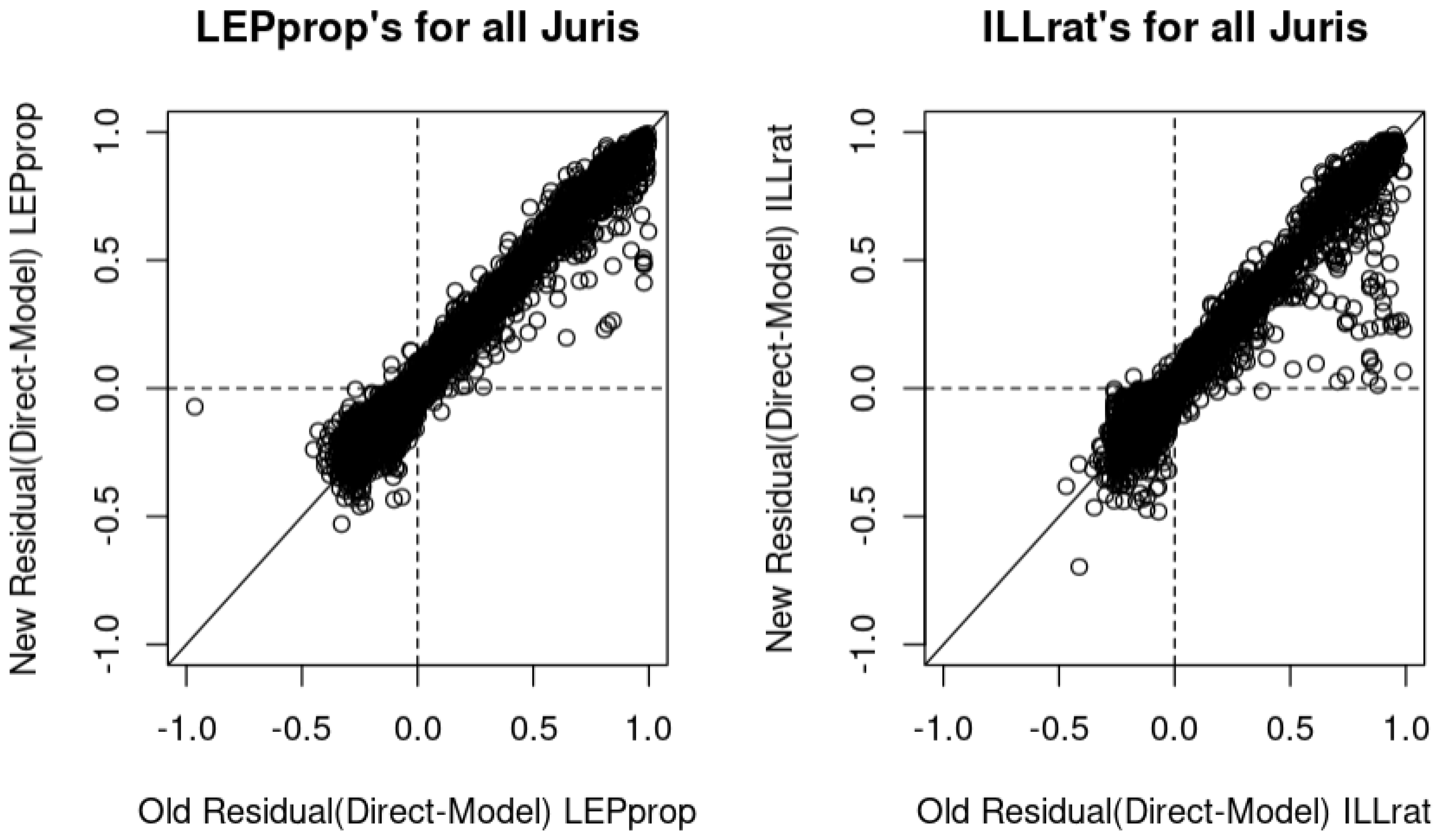
Figure 1 compares the performance of the old and new models. Each point represents a jurisdiction across all 73 LMGs. The residual value here is the difference between “Direct” and "Model" estimates. LEPprop denotes the proportion of voting-age citizens who have limited English proficiency (or LEP / CIT), while ILLrat represents the illiteracy rate among citizens with limited English proficiency (or ILL / LEP). If all the points in this residual plot were on the 45-degree line, that would indicate that there was no difference between the old and new models. The closer the points are to a horizontal line in the center of the plot, the better the new model is performing for those jurisdictions. The fact that both plots show several points below the 45-degree lines and above the horizontal line at the center indicates that the old model has larger residuals than the new model for those jurisdictions. This pattern is consistent through all sample size bins.
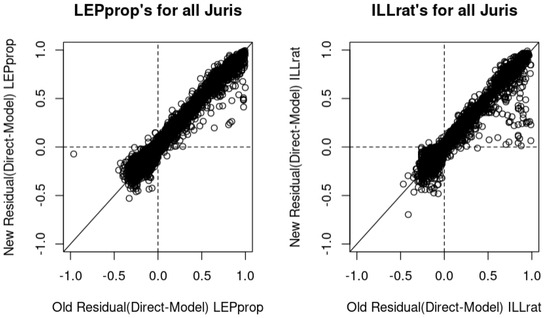
Figure 1.
Residual plots.
5. Discussion
In this paper, a new statistical methodology was proposed for the Bayesian multinomial logit model for US Voting Rights Act Section 203 determinations. Our methodological contribution involved adopting PG augmentation to linearize the nonlinear optimization problem, resulting in closed-form solutions for posterior distributions. This enhanced computational stability in the Gibbs sampling steps, which enabled us to fit one model for all jurisdictions. The former 2021 VRA determinations used different models for different jurisdictions—that is, if one model did not fit, then other models were tried for the same jurisdiction data.
Our method was developed based on the works of George and McCulloch [8] and Polson et al. [6]. George and McCulloch [8] did not suggest formal convergence criteria or diagnostics. Instead, they relied on empirical observations of convergence. Polson et al. [6] implemented the PG sampling algorithm in the R package BayesLogit. Note that while convergence diagnostics such as trace plots can indicate non-convergence, they cannot definitively prove convergence, especially given the substantial number of parameters in our analysis. The ultimate evidence of convergence was the improvement in the new model’s diagnostic measures over the 2021 VRA model.
Using SSVS requires the specification of the prior parameters and . Setting to 0.5 and to 10 produced desirable diagnostic results for all LMGs, as discussed in Section 4. In exchange for the additional effort required to identify suitable SSVS priors, the new PG-based Bayesian model demonstrates improved efficiency compared to the previous STAN-based Bayesian model developed for the 2021 VRA project. For example, the new model produced parameter estimates for the Bangladeshi LMG’s 517 jurisdictions in approximately 8 min. In contrast, the 2021 Bayesian VRA model for this LMG could not be estimated at all using STAN. The use of other Bayesian variable selection procedures, such as Bayesian LASSO [9], is a topic of interest for future research.
The estimates from the new model can be viewed as Bayesian model averages, because the posterior parameters were sampled and averaged over various models that had different sets of selected covariates. The overall results for the 2021 VRA data showed that the new model, which used stochastic search variable selection(SSVS) [8] separately in each LMG, outperformed the previous model, which used the same covariates in every LMG. The diagnostic data presented for the Bangladeshi and Sri Lankan LMGs are examples of how the new model yielded better results than the 2021 VRA models, especially in jurisdictions with small sample sizes of between one and four voting-age persons.
The nonlinearity of the logistic link function of the MLN model and the unseen latent random effects variables were computationally challenging issues. Both the frequentist adaptive Gaussian quadrature procedure and Bayesian inference can handle random effects, as was demonstrated in previous 2021 VRA determinations [1]. The frequentist model was fit by using adaptive Gaussian quadrature to optimize the likelihood function, which required the random effects variable to be averaged out. This approach makes it technically difficult to adopt variable selection procedures, since the entire score function would have to be modified for such an additional procedure. In contrast, Bayesian methods treat the random effects as just another parameter, which can be drawn in Gibbs sampling. STAN was used to sample the random effects and their covariance matrix for the 2021 VRA Bayesian model, but it did not converge for smaller LMGs. Our new Bayesian model used PG augmentation to obtain closed-form solutions for posterior distributions, which made implementing Bayesian stochastic search variable selection computationally feasible in more LMGs. This lead to noticeable improvements in our overall diagnostic results.
Author Contributions
Conceptualization, J.K. and A.C.H.; data curation, A.C.H.; formal analysis, J.K. and A.C.H.; methodology, J.K.; project administration, J.K.; software, J.K. and A.C.H.; supervision, J.K.; validation, J.K.; visualization, J.K.; writing—original draft preparation, J.K.; writing—review and editing, A.C.H. All authors have read and agreed to the published version of the manuscript.
Funding
This research received no external funding.
Data Availability Statement
The datasets presented in this article are not readily available because they are protected by Title 13, U.S.C., in the interests of respondent privacy.
Conflicts of Interest
The authors declare no conflicts of interest.
Appendix A. Derivation of the Posterior [6]
Without loss of generality, we omit the outcome category indicator k from variable notations in this section. This means that will be written as , will be written as U, will be written as , etc. Recall that Z=, denote , and suppose is sampled from . Then, is proportional to
where is + and is +. Note that is because is such that = 0, where = and because is the same as .
Thus, the posterior distribution of |Z,X is
where is + and is + , which is + , where = .
Appendix B. Derivation of the Posterior for the VRA Model
Without loss of generality, we omit the outcome category indicator k from variable notations in this section. This means that will be written as , will be written as U, will be written as , etc. Recall X is the matrix of covariates. Let U denote the matrix of random effects variables, denote a standard normal prior for , and the likelihood function denote . Then, is proportional to
where is + and is + , denotes for a variable A, and y and n denote ,…, and ,…,, respectively, as described in Section 2. Note that is − because is such that = 0, and hence = . Now, is and − . Thus, − = .
Appendix C. Derivation of
Let us assume a Gaussian prior distribution for the random effects variables (=,,) for jurisdiction j. Recall that denoted the counts of persons with language conditions. The conjugate Gaussian posterior for is proportinal to , as shown as follows.
where = + , = , = , = − , = , = , and = , and + . The last two lines of the equations result by the algebra in Appendix E.
Appendix D. Derivation of
Assume a multivariate normal distribution on U, which is
An inverse Wishart for the prior distribution with known scale matrix and the degrees of freedom for a covariance matrix is
The conditional posterior is proportional to
Appendix E. Algebraic Basics: Sum of Quadratic Matrices
Appendix E.1. Sum of Two Quadratic Matrices
Appendix E.2. Sum of N Quadratic Matrices
Consider x to be a vector of the VRA’s three disjoint outcomes. Then,
= and = . Thus, .
References
- Slud, E.V.; Franco, C.; Hall, A.; Kang, J. Statistical Methodology (2021) for Voting Rights Act, Section 203 Determinations. 2022. Available online: https://www.census.gov/library/working-papers/2022/adrm/RRS2022-06.html (accessed on 9 April 2024).
- Joyce, P.M.; Malec, D.; Little, R.J.; Gilary, A.; Navarro, A.; Asiala, M.E. Statistical Modeling Methodology for the Voting Rights Act Section 203 Language Assistance Determinations. J. Am. Stat. Assoc. 2014, 109, 36–47. [Google Scholar] [CrossRef]
- Slud, E.V.; Ashmead, R.; Joyce, P.; Wright, T. Statistical Methodology (2016) for Voting Rights Act, Section 203 Determinations. 2018. Available online: https://www.census.gov/library/working-papers/2018/adrm/RRS2018-12.html (accessed on 9 April 2024).
- Pinheiro, J.C.; Bates, D.M. Approximations to the Log-Likelihood Function in the Nonlinear Mixed-Effects Model. J. Comput. Graph. Stat. 1995, 4, 12–35. [Google Scholar] [CrossRef]
- Carpenter, B.; Gelman, A.; Hoffman, M.D.; Lee, D.; Goodrich, B.; Betancourt, M.; Brubaker, M.; Guo, J.; Li, P.; Riddell, A. Stan: A probabilistic programming language. J. Stat. Softw. 2017, 76, 1–32. [Google Scholar] [CrossRef] [PubMed]
- Polson, N.G.; Scott, J.G.; Windle, J. Bayesian Inference for Logistic Models Using Polya Gamma Latent Variables. J. Am. Stat. Assoc. 2013, 108, 1339–1349. [Google Scholar] [CrossRef]
- Polson, N.G.; Scott, J.G.; Windle, J. Package: BayesLogit 2.1. 2019. Available online: https://cran.r-project.org/web/packages/BayesLogit/index.html (accessed on 9 April 2024).
- George, E.I.; McCulloch, R.E. Variable Selection via Gibbs Sampling. J. Am. Stat. Assoc. 1993, 88, 881–889. [Google Scholar] [CrossRef]
- Park, T.; Casella, G. The Bayesian Lasso. J. Am. Stat. Assoc. 2008, 103, 681–686. [Google Scholar] [CrossRef]
Disclaimer/Publisher’s Note: The statements, opinions and data contained in all publications are solely those of the individual author(s) and contributor(s) and not of MDPI and/or the editor(s). MDPI and/or the editor(s) disclaim responsibility for any injury to people or property resulting from any ideas, methods, instructions or products referred to in the content. |
© 2025 by the authors. Licensee MDPI, Basel, Switzerland. This article is an open access article distributed under the terms and conditions of the Creative Commons Attribution (CC BY) license (https://creativecommons.org/licenses/by/4.0/).