Article

Evaluating the Discrete Generalized Rayleigh Distribution: Statistical Inferences and Applications to Real Data Analysis

by
Hanan Haj Ahmad
1,*,
Dina A. Ramadan
2 and
Ehab M. Almetwally
3,4,*
1
Department of Basic Science, The General Administration of Preparatory Year, King Faisal University, Hofuf 31982, Al Ahsa, Saudi Arabia
2
Department of Mathematics, Faculty of Science, Mansoura University, Mansoura 33516, Egypt
3
Department of Mathematics and Statistics, Faculty of Science, Imam Mohammad Ibn Saud Islamic University (IMSIU), Riyadh 11432, Riyadh, Saudi Arabia
4
Faculty of Business Administration, Delta University of Science and Technology, Gamasa 11152, Egypt
*
Authors to whom correspondence should be addressed.
Mathematics 2024, 12(2), 183; https://doi.org/10.3390/math12020183
Submission received: 10 December 2023 / Revised: 30 December 2023 / Accepted: 3 January 2024 / Published: 5 January 2024
(This article belongs to the Special Issue Application of the Bayesian Method in Statistical Modeling)

Abstract

:
Various discrete lifetime distributions have been observed in real data analysis. Numerous discrete models have been derived from a continuous distribution using the survival discretization method, owing to its simplicity and appealing formulation. This study focuses on the discrete analog of the newly generalized Rayleigh distribution. Both classical and Bayesian statistical inferences are performed to evaluate the efficacy of the new discrete model, particularly in terms of relative bias, mean square error, and coverage probability. Additionally, the study explores different important submodels and limiting behavior for the new discrete distribution. Various statistical functions have been examined, including moments, stress–strength, mean residual lifetime, mean past time, and order statistics. Finally, two real data examples are employed to evaluate the new discrete model. Simulations and numerical analyses play a pivotal role in facilitating statistical estimation and data modeling. The study concludes that the discrete generalized Rayleigh distribution presents a notably appealing alternative to other competing discrete distributions.

1. Introduction

As each day passes, the volume of data in our world increases exponentially, necessitating the development of new statistical distributions to better characterize the features of many phenomena and experiments. While a great deal of lifetime data appear to be continuous, they are originally discrete. This discrepancy ensures the need for more appropriate methods to generate discrete distributions that more accurately represent the data in the experiment. Discrete distributions are frequently employed in statistical modeling for several reasons.
Discrete distributions are used to model data that can only take on a finite or countably infinite number of values, such as counts, proportions, and binary outcomes, for example, the number of customers in a store, the number of heads in a coin flip, or the number of defective items in a production line. Discrete distributions are often easy to understand and interpret as they model data that take on a limited number of values. The probability mass function (pmf) or probability generating function (pgf) of a discrete distribution is a simple function that provides the probability of each possible outcome. Also, many discrete distributions have closed-form expressions for their pmf or pgf, which makes it easy to work with them mathematically. This allows for efficient computation of probabilities and moments without the need for integration. Furthermore, discrete distributions can be used to model a wide variety of real-world phenomena, such as the distribution of species in an ecosystem, the distribution of genetic variations in a population, or the distribution of traffic on a road network.
Recently, many discrete distributions have been considered, particularly in medicine, engineering, reliability, survival analysis, and more. For more descriptions and applications of discrete distributions, refer to [1,2,3,4,5,6,7,8,9]. Hence, many authors have conducted much work to originate and develop discrete models from different aspects.
The characterization of continuous random variables can be performed either by their probability density function, cumulative distribution function, moments, moment-generating function, hazard rate functions, or others. Different discretization methods appeared in the literature to create an appropriate discrete distribution based on the underlying continuous model.
By deriving discrete analogs or counterparts of well-known continuous distributions, statisticians can better tailor their models to the specific nature of the data. Usually, creating a discrete analog from a continuous distribution is based on the principle of preserving one or more characteristic properties of the continuous one. Consequently, different ways to discretize a continuous distribution appear in the literature depending on the property the researcher intends to preserve; for example, Lai [10] used the survival and the hazard rate preservation methods to create discrete distributions from different continuous ones. Haj Ahmad and Almetwally [11] used the survival, hazard rate, and probability distribution function preservation methods to discretize the generalized Pareto distribution.
The benefit of using the survival discretization method is that it can maintain the statistical properties of the original distribution, including median and percentiles, in addition to the overall shape of the distribution. A drawback of this method is that it can be computationally intensive and may require numerical methods for complex distributions.
For the hazard preservation method, the main benefit is that it preserves the hazard function of the continuous distribution. This is important in applications like reliability analysis where the failure rate is a key parameter. On the other hand, mathematical complexity can be viewed using this method, especially for continuous distributions with nonlinear hazard functions. This complexity can increase computational time and resource requirements. Another drawback of the hazard preservation method is that it only preserves the hazard function, but other characteristics of the distribution (like mean, variance, or skewness) may not be as accurately retained. For more details about other discretization methods and their properties, one may refer to [12,13] who provided a review of several discretization methods.
From the previous research work, it is evident that the results look appealing and motivational to continue creating new discrete distributions to model new data.
In the present study, we obtain a discrete analog of the continuous new generalized Rayleigh distribution (NGRD) using the survival discretization method that depends on the survival function. See for example [6,7], in which the survival discretization approach was used to obtain the discrete normal and discrete Rayleigh distributions, respectively. Using the same approach, more discrete distributions have been introduced and studied; see for example [14,15,16,17,18,19,20,21,22,23].
Still, there is an enduring need to create and develop more discrete models and to generate new ones because of modeling and fitting real data, which appear and spread constantly in human life. The efficiency in discretization methods refers to the ability of a method to produce accurate and useful discretized versions of continuous data with minimal loss of information. Also, discrete distributions derived from continuous ones can inherit their flexibility and adaptability. This allows statisticians to model a wider range of data characteristics, such as skewness or kurtosis, which might be difficult with standard discrete distributions. In statistical methodology, continuous distributions may have characteristics that are missing in the discrete space; hence, creating discrete analogs can fill these gaps, providing new tools for data analysis.
The suggested discrete model with three parameters offers an immense degree of fitness to skewed, symmetric, monotone, and inverse J-shape types of data. Therefore, some statistical functions and properties are achieved, in addition to observing the submodels and limiting behavior of the proposed discrete distribution. Examining statistical inference is crucial; therefore, point and interval estimation for the unknown parameters using the maximum likelihood estimator and the Bayesian method is performed.
Simulation analysis via numerical techniques such as Monte Carlo simulation is employed to evaluate the estimators using the maximum likelihood and the Bayesian estimation methods to compare the performance of these two methods. The efficiency is assessed using the relative bias, the mean squared error, and the coverage probability of the confidence intervals. Two real datasets are analyzed to emphasize the empirical validation of the new model, where several goodness-of-fit measures are employed. The first example is related to the industrial field, where several strikes that occurred in coal mining in the UK were recorded over four weeks. Modeling and predicting the number of strikes will save human lives and money. The second example is related to the number of fires that occurred in Greece’s forests in the year 1998 during the summer months. The main purposes of this study are, first, to introduce new discrete analogs of the continuous NGRD and evaluate some of its important statistical functions, second, to perform the inferential statistics related to the new distributions’ parameters and compare the results, and, third, to assess the efficiency of the new discrete distribution by modeling real data examples and comparing the goodness-of-fit measures with other discrete distributions that were studied earlier in the literature.
The originality of this work emanates from the basis of exploring the creation of a new discrete analog from less commonly used continuous distributions and investigating their properties, potential applications, and how they compare to existing distributions. Also, it focuses on specific application areas, such as the industrial, engineering, and reliability fields. To our knowledge, no previous work has studied the discrete new generalized Rayleigh distribution and employed it to model real-life data examples from different scientific fields.
The authors’ contributions to this study can be summarized as follows:
  • Development of a New Discrete Model: Creation of a discrete analog of the continuous new generalized Rayleigh distribution (NGRD) using the survival discretization method.
  • Statistical Functions and Properties: Achievement of various statistical functions and properties of the proposed discrete distribution, including observing its submodels and limiting behavior.
  • Statistical Inference Examination: Conducting point and interval estimation for the unknown parameters using both the maximum likelihood estimator (MLE) and the Bayesian method.
  • Simulation Analysis for Estimator Evaluation: Implementation of numerical techniques such as Monte Carlo simulation to evaluate the estimators derived from MLE and Bayesian estimation methods through relative bias, mean squared error, and coverage probability of confidence intervals
  • Empirical Validation via Real Data Analysis: Analyzing two real datasets to validate the new model empirically, including modeling industrial and environmental phenomena.
  • Comparison with other Distributions: Comparing the goodness of fit of the new model with other discrete distributions previously studied in the literature.
The remaining parts of this work are organized as follows: Section 2 describes the new generalized Rayleigh distribution. The discretization methods are presented in Section 3, along with some statistical functions. In Section 4, the maximum likelihood and the Bayesian inference are presented. In Section 5, simulation analysis and the tabulated results are carried out. Some real data examples are provided in Section 6. Finally, conclusions are remarked on in Section 7.

2. Model Description

The Rayleigh distribution (RD) is a continuous distribution that has much practical importance; hence, many of its statistical characteristics, inference, and reliability analysis have been studied by several authors, and numerous extended forms of the Rayleigh distribution have been proposed. For example, Ref. [24] applied the inverse Rayleigh to the failure times data. Ref. [25] introduced the transmuted Rayleigh and used it to model the amount of nicotine in the blood. In [26], the authors studied the beta-generalized Rayleigh distribution and its application. Ref. [27] obtained the transmuted inverse Rayleigh distribution to lifetime data. Ref. [28] obtained a new modified Rayleigh distribution named the Kumaraswamy generalized Rayleigh distribution with application to real data. For more information, refer to [29,30,31]. In this work, we are interested in studying a new form of the Rayleigh distribution called a new generalized Rayleigh distribution (NGR), which was first introduced by Shen et al. [32]. It has three parameters and it was shown that the NGR is suitable for modeling large data values rather than small data values. However, as a continuous distribution, it is restricted from describing discrete data forms. Discretizing the NGR distribution is our goal; therefore, it yields a subsequent distribution that accommodates the countable data while retaining the influential tail modeling characteristics of the NGR. In this study, we carry out a discrete version of the NGR and use it to model real data.
The probability density function (pdf) and the survival function (S) of the continuous NGR are provided respectively as:
f x ; α , β , θ = 2 α β θ α 1 x e θ x 2 ( 1 e θ x 2 ) β 1 α 1 e θ x 2 β 2 , x > 0 ,
and
S x ; α , β , θ = α [ 1 1 e θ x 2 β ] α 1 e θ x 2 β ,
in which the parameters α > 1 , β > 0 , θ > 0 .
The hazard rate function is
h x ; α , β , θ = 2 β θ α 1 x e θ x 2 ( 1 e θ x 2 ) β 1 1 1 e θ x 2 β α 1 e θ x 2 β 2 .
To identify submodels or special distributions that arise from this general form, we can consider different values or limits of parameters α , β , and θ . Here are some special cases:
  • Standard Rayleigh Distribution: When θ = 1 and β = 1 , the term ( 1 e x 2 ) simplifies to the CDF of the standard Rayleigh distribution. This is observed if the parameter α also approaches infinity, which simplifies the formula to 1 e x 2 , the CDF of the standard Rayleigh distribution.
  • Exponential Distribution: If β approaches infinity, the term Λ = ( 1 e θ x 2 ) β can approach an exponential-like behavior for small values of x, depending on how θ is defined.
  • Modified Rayleigh Distribution: For specific fixed values of α and β , you can obtain various forms of modified Rayleigh distributions, where the behavior is measured by the degree of skewness and kurtosis determined by these parameters.
  • Weibull-like Distribution: By interchanging between θ and β , especially when β is not equal to 1, the distribution can possess Weibull-like properties.
By discretizing the continuous range of x, discrete versions of this distribution can be derived, which may be useful for certain types of count data or integer-valued measurements.
Since our goal in this work is to define a new discrete NGR distribution, we generate a discrete analog based on the survival discretization method, which is denoted by DNGR. The pmf and cumulative distribution function (CDF) are obtained. Furthermore, the moments, stress–strength function, the mean residual, and mean past lifetimes, order statistics, and L-moments are obtained. All these statistical functions are used for studying the features of the DNGR.

3. The Discrete New Generalized Rayleigh Distribution

Roy and Gupta [3,4] defined the probability mass function (pmf) for a discrete distribution using the survival function and it was expressed as follows:
P X = k = S k S k + 1 , k = 0 , 1 , 2 ,
where S x is the survival function provided by Equation (2); hence, the pmf of the discrete analog of NGR distribution, namely DNGR, is written as
P X = k = α [ 1 Λ k ; θ , β ] α Λ k ; θ , β α 1 Λ k + 1 ; θ , β α Λ k + 1 ; θ , β ,
where Λ k ; θ , β = 1 e θ k 2 β .
The CDF of the DNGR distribution can be written as
P X < k = F k + 1 = 1 α 1 Λ k + 1 ; θ , β α Λ k + 1 ; θ , β .
The quantile function with given values of parameters as α , β , and θ of the DNGR distribution is provided by
x i = 1 θ ln 1 α q α + q 1 1 / β 1 ; q = [ 0 , 1 ] , i = 1 , , n .
The hazard rate function (HRF) of the DNGR distribution is provided by
h DNGR 1 k = 1 Λ k ; θ , β α Λ k + 1 ; θ , β α Λ k ; θ , β 1 Λ k + 1 ; θ , β 1 .
We also observe that the reversed hazard rate function for the DNGR of this distribution is provided by
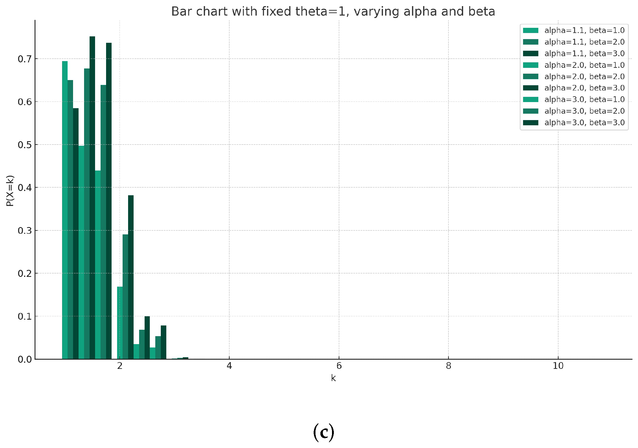
r D N G R k ; α , β , θ = f k ; α , β , θ F k + 1 ; α , β , θ ,
r D N G R k ; α , β , θ = α 1 Λ k ; θ , β α Λ k ; θ , β α 1 Λ k + 1 ; θ , β α Λ k + 1 ; θ , β × α Λ k + 1 ; θ , β α Λ k + 1 ; θ , β α 1 Λ k + 1 ; θ , β
In Figure 1, the bar charts represent each parameter α , θ , and β that has a specific role in the behavior of the pmf, and their effects are observable when we fix one and vary the others. An explanation of the effect of each parameter based on the plots is as follows:
1.
Effect of α when θ and β are changeable:
When α is fixed, the variations in θ and β create different trends in the probability values. Higher values of θ tend to stretch the curve horizontally, meaning, for a given α , as θ increases, the decrease in probability values with increasing k is less steep. Higher values of β tend to amplify the curve vertically, making the probability have fewer values for higher k values. The reaction between θ and β at a fixed α demonstrates that θ affects the spread of the distribution, while β affects the sharpness of the probability decrease.
2.
Effect of θ when α and β are changeable:
With θ fixed, the changes in α and β show distinct patterns. An increase in α generally results in higher probability values across all k. This is because a higher α relative to Λ (k; θ , β ) increases the numerator and decreases the denominator of the function P ( X = k ) , resulting in a larger overall value. The effect of β at a fixed θ is similar to its effect when α is fixed; it controls the sharpness of the decrease in probability values. Higher β values cause a quicker decline in probability as k increases.
3.
Fixing β and varying α and θ , we can see that
As α increases, for a fixed β , the overall probability values increase, similar to when θ is fixed. The role of θ here is nuanced; for lower values of k, the impact of changing θ is minimal, but, as k increases, higher θ values preserve higher probabilities, indicating a wider spread in the distribution. From the above explanations, it is clear that α primarily scales the probability values, β determines the rate at which the probability values decline as k increases (sharpness of the distribution), and θ controls the spread or dispersion of the distribution across k values. The combination of these three parameters can thus shape the function’s distribution in various ways, and each has a distinctive role in the form of the probability curve.
In Figure 2, the plots represent the HRF of the DNGR distribution for various combinations of parameters α , θ , and β . Each subplot corresponds to a different set of these parameters. The values of k range from 1 to 10. The curves are increasing for different values of the parameters; we can realize the effect of increasing the parameter θ while keeping other parameters fixed by going steeply to the left. For the effect of β , assuming other parameters are fixed, it can be figured by increasing in a slower mode when k takes small values. Finally, the effect of increasing the values of α while fixing the remaining parameters is going to the left more steeply.
The limiting behavior of DNGR for different choices in parameter values at the boundary points includes
lim k p k = 0 , lim k 0 p k = 0 ,
lim α 1 p k = 0 , lim α p k = Λ k + 1 ; θ , β Λ k ; θ , β ,
lim θ 0 p k = 0 , lim θ p k = 0 ,
lim β 0 p k = 0 , and lim β p k = 0 .
From the above limiting behavior of the DNGR, some submodels and special cases can be derived, such as
  • Discrete standard Rayleigh Distribution: When θ = 1 and β = 1 , and α approaches infinity, the pmf simplifies to ( 1 e ( x + 1 ) 2 ) ( 1 e x 2 ) , which represents the pmf of the discrete Rayleigh distribution created from applying the survival discretization method.
  • Discrete Exponential-like Distribution: For large values of β and specific values of θ , the DNGR distribution might possess characteristics similar to an exponential distribution for smaller values of k, where the exponential decay behavior is more evident, since the term Λ = ( 1 e θ k 2 ) β has a decaying form and can be considered as exponential-like function.
  • Discrete Uniform Distribution: If the parameters α , β , and θ are chosen such that the pmf becomes constant for all k within a certain range, the DNGR distribution could approximate a discrete uniform distribution.
  • Geometric-like Distribution: By adjusting θ and β , you might be able to create a distribution that behaves like the geometric distribution, especially if the probability of larger k values decays like the geometric series.
These possible submodels and special cases demonstrate the versatility and adaptability of the DNGR distribution. The ability to derive such a variety of distributions from a single distribution highlights the potential utility of the DNGR distribution in modeling a wide range of discrete data scenarios. Each submodel or special case would be suited to different types of data and could provide unique insights depending on the context of the analysis.

3.1. Moments

Assume a non-negative random variable k D N G R α , β , θ . The s t h moment, say ψ s , can be expressed as follows
ψ s = k = 0 k s f k ; α , β , θ ,
and then
ψ s = k = 0 k s α 1 Λ k ; θ , β α Λ k ; θ , β α 1 Λ k + 1 ; θ , β α Λ k + 1 ; θ , β .
It is impossible to write an exact form of the s t h moment; hence, R programming with version (4.3.0) is helpful, and the moment is evaluated numerically. Equation (11) is convergent for α > 1 , β > 0 , and θ > 0 .
Table 1 explores some functions like the minimum, mean, variance, maximum, skewness (SK), and kurtosis (Kt) for different values of α , β , and θ . In addition, the DNGR distribution is appropriate for modeling both over- and under-dispersed data since, in this model, the variance can be smaller than the mean, which is the case with some standard classical discrete distributions, in addition to the positive and negative skewness values, which show that this distribution can be skewed to the right or left. Also, a very small skew value that tends to zero indicates a symmetry possible curve for the pmf. A higher kurtosis means more of the variation is due to infrequent extreme deviations as opposed to frequent modestly sized deviations. By varying θ , α , and β , one can realize the distribution changes. For instance, with θ = 0.8 and α = 0.5, β changing from 0.84 to 2.73 drastically increases the kurtosis, indicating a heavier tail.

3.2. Stress–Strength Analysis

The stress–strength (reliability) analysis is an important tool in mechanical design. The idea relies on the probability of failure that is obtained from the probability of r exceeding r * . Assume that both r and r * are in the positive domain. The expected reliability ( R * ) can be calculated by
R * = P K r K r * = k = 0 f K r k R K r * k ,
in which K r D N G R α 1 , β 1 , θ 1 and K r * D N G R α 2 , β 2 , θ 2 , and then R * can be expressed as follows
R * = k = 0 α 1 1 Λ 1 k ; θ 1 , β 1 α 1 Λ 1 k ; θ 1 , β 1 α 1 1 Λ 1 k + 1 ; θ 1 , β 1 α 1 Λ 1 k + 1 ; θ 1 , β 1 α 2 1 Λ 2 k ; θ 2 , β 2 α 2 Λ 2 k ; θ 2 , β 2 ,
where Λ 1 k ; θ 1 , β 1 = 1 e θ 1 k 2 β 1 and Λ 2 k ; θ 2 , β 2 = 1 e θ 2 k 2 β 2 .
We cannot obtain a closed form for the above equation; consequently, simulation analysis is utilized to obtain a numerical solution. In Section 6, numerical analysis is performed to obtain the value of the stress–strength function under two real data applications.

3.3. The Mean Residual and the Mean Past Lifetimes

In reliability and survival analysis, many lifetime measures have been discussed in the literature. They were defined to study the aging behavior of the experimental units. One of these measures is the mean residual lifetime (MRL), which is a helpful tool in determining burn-in and maintenance policies. For discrete distributions, the MRL is defined as follows:
ζ i = E k i k i k i k i = 1 S i j = i + 1 l S j ; i N ,
where 0 < l < .
If the random variable k follows the DNGR distribution with parameters α , β , and θ , which is denoted by k D N G R α , β , θ , then the MRL is expressed as
ζ i = α Λ i ; θ , β α 1 Λ i ; θ , β j = i + 1 l α 1 Λ j ; θ , β α Λ j ; θ , β .
The mean past lifetime (MPL) is another important measure in reliability analysis. The MPL measures the time elapsed after the failure of K units given that the system has failed sometime earlier to i. In the discrete case, the MPL is defined as follows
ζ * i = E i k | k < i = 1 F i 1 m = 1 i F m 1 ; i N 0 ,
where ζ * 0 = 0 ; see [33].
Then,
ζ * i = 1 α Λ i ; θ , β α 1 Λ i ; θ , β 1 m = 1 i 1 α 1 Λ m 1 ; θ , β α Λ m 1 ; θ , β .

3.4. Order Statistics

Let K 1 , K 2 , , K n be a random sample with the DNGR distribution and K 1 : n , K 2 : n , , K n : n denote the corresponding order statistics. Then, the CDF of i t h order statistics at the value k can be written as follows
F i : n k ; α , β , θ = i = 1 n n m F i k ; α , β , θ m 1 F i k ; α , β , θ n m .
By using the negative binomial theorem, then
F i : n k ; α , β , θ = i = 1 n j = 1 n m n m n m j 1 j F i k ; α , β , θ m + j .
Therefore,
F i : n k ; α , β , θ = i = 1 n j = 1 n m n m n m j 1 j 1 α 1 Λ k ; θ , β α Λ k ; θ , β m + j .
Consequently, the pmf of the i t h order statistic under the DNGR can be derived and expressed as follows
f i : n k ; α , β , θ = i = 1 n j = 1 n m n m n m j 1 j α 1 Λ k ; θ , β α Λ k ; θ , β α 1 Λ k + 1 ; θ , β α Λ k + 1 ; θ , β m + j .
So, the υ t h moments of k i : n can be written as follows
E ( K i : n ν ) = k = 0 i = 1 n j = 1 n m n m n m j 1 j k ν α 1 Λ k ; θ , β α Λ k ; θ , β α 1 Λ k + 1 ; θ , β α Λ k + 1 ; θ , β m + j .

4. Estimation

Two estimation methods are considered in this work: frequentist maximum likelihood estimation (MLE) and the Bayesian estimation method. Simulation analysis and numerical techniques are performed in Section 5 to assess the performance of these estimation methods.

4.1. Maximum Likelihood Estimation

In this section, we use the maximum likelihood estimation MLE method to estimate the unknown parameters of the DNGR distributions. To evaluate the required estimators, numerical techniques are used, such as the well-known Newton–Raphson technique.
Let x 1 , , x n be a random sample following the DNGR, and then, from pmf in Equation (5), the log-likelihood function is written as
α , β , θ = k = 1 n log α α 1 + log Λ x k + 1 ; θ , β Λ x k ; θ , β log α Λ x k ; θ , β log α Λ x k + 1 ; θ , β
The MLEs for α , β , and θ are obtained by finding the partial derivatives of α , β , θ for α , β , and θ , then equating the three equations to zero and solving numerically.
α , β , θ α = k = 1 n 2 α 1 α α 1 1 α Λ x k ; θ , β 1 α Λ x k + 1 ; θ , β = 0 ,
α , β , θ β = k = 1 n Λ β x k + 1 ; θ , β Λ β x k ; θ , β Λ x k + 1 ; θ , β Λ x k ; θ , β + Λ β x k ; θ , β α Λ x k ; θ , β + Λ β x k + 1 ; θ , β α Λ x k + 1 ; θ , β = 0
and
α , β , θ θ = k = 1 n Λ θ x k + 1 ; θ , β Λ θ x k ; θ , β Λ x k + 1 ; θ , β Λ x k ; θ , β + Λ θ x k ; θ , β α Λ x k ; θ , β + Λ θ x k + 1 ; θ , β α Λ x k + 1 ; θ , β = 0 .
Such that Λ β x k ; θ , β = Λ x k ; θ , β β = Λ x k ; θ , β log ( 1 e θ x k 2 ) and Λ θ x k ; θ , β = Λ x k ; θ , β θ = β x k 2 e θ x k 2 Λ x k ; θ , β 1 . To solve the system of nonlinear Equations (21)–(23), only numerical methods are helpful. Many numerical techniques were used in the literature; here, we use the Newton–Raphson method, and all results are illustrated in Section 5.

4.2. Bayesian Inference

The Bayesian estimation method is used in this section to estimate the unknown parameters of the DNGR. The basic assumption of the Bayesian method is that the model parameters are considered random variables that follow a distribution known as the prior distribution. Since prior information is usually only available, we must specify a suitable prior option. We choose the gamma conjugate prior distribution for the parameters α , β , and θ . It is defined by assuming gamma distributions for α , β , and θ .
Therefore, the prior distributions for α , β , and θ can be written as
π 1 ( α ) = b 1 a 1 Γ ( a 1 ) α a 1 1 e b 1 α ,
π 2 ( β ) = b 2 a 2 Γ ( a 2 ) β a 2 1 e b 2 β
and
π 3 ( θ ) = b 3 a 3 Γ ( a 3 ) θ a 3 1 e b 3 θ
where a 1 , a 2 , a 3 , b 1 , b 2 , and b 3 are nonnegative hyper parameters of the assumed distributions.
Hence, the joint prior for α , β , and θ is
π ( α , β , θ ) α a 1 1 β a 2 1 θ a 3 1 e ( b 1 α + b 2 β + b 3 θ ) .
The joint posterior of α , β , and θ given the data is defined as
π * α , β , θ x = 1 k L ( x ̲ α , β , θ ) π ( α , β , θ ) ,
where L ( x ̲ α , β , θ ) is the likelihood function of the DNGRD and K = L ( x ̲ α , β , θ ) π ( α , β , θ ) d α d β d θ .
The DNGRD parameters are estimated using a symmetric squared error (SE) loss function. A simulation study is used to investigate the performance of the estimators using the aforementioned loss function. As criteria for the superiority of the estimation methods, the bias, the mean square error (MSE), the average length (AL) of the confidence intervals, and the coverage probability (CP) are computed.
Under the SE loss function, Bayes estimation for the parameters α , β , and θ is defined as the mean or expected value regarding the joint posterior, provided as
α ^ S E = 1 k α L ( x ̲ α , β , θ ) π ( α , β , θ ) d α d θ
β ^ S E = 1 k β L ( x ̲ α , β , θ ) π ( α , β , θ ) d α d θ
θ ^ S E = 1 k θ L ( x ̲ α , β , θ ) π ( α , β , θ ) d α d θ
To evaluate the expected values and triple integration in Equations (26)–(28), numerical methods are required. We choose to use the Markov chain Monte Carlo (MCMC) technique via the Gibbs sampling method and by developing appropriate R code. The joint posterior density is
π * ( α , β , θ x ̲ ) = 1 K i = 1 n [ 1 Λ i ; θ , β ] α Λ i ; θ , β 1 Λ i + 1 ; θ , β α Λ i + 1 ; θ , β α a 1 β a 2 1 θ a 3 1 e ( b 1 α + b 2 β + b 3 θ )
Bayes estimation for parameters α , β , and θ under SE loss function is performed respectively using Equations (26)–(28) and the posterior density Equation (29).
The estimators are numerically evaluated simulations using R codes under the SE loss function, and their results are summarized and presented in Table 2 and Table 3.

5. Simulation Analysis

In this section, Monte Carlo simulations are performed to assess the effectiveness of the suggested estimators for the parameters α , θ , and β that were established in Section 4.1. We will sum up by providing the simulation scenario. The findings of the simulation are then offered for debate.

5.1. Simulation Scenario

In this subsection, several Monte Carlo simulation studies are carried out to assess the effectiveness of the acquired maximum likelihood estimates and Bayesian estimation of α , θ , and β . Now, we suggest the following steps to gather a sample from the DNGR model:
  • Set α , θ , and β to their actual values as shown:
    In Table 2: α = 1.5 , θ = 0.8 , β = 0.5 , α = 1.5 , θ = 0.8 , β = 2 , α = 1.5 , θ = 1.3 , β = 0.5 , α = 1.5 , θ = 1.3 , β = 2 .
    In Table 3: α = 3 , θ = 1.3 , β = 0.5 , α = 3 , θ = 1.3 , β = 0.9 , α = 3 , θ = 2 , β = 0.5 , α = 3 , θ = 2 , β = 1.1 .
  • Specific values for n (total test units) should be determined as 30, 70, 100, 200.
  • Generate a uniform random variable within the range of 0 to 1. Utilize the quantile function described in Equation (7) to produce a random sample from the DNGR ( α , θ , β ) distribution. Afterwards, round the quantity of samples to the nearest whole number.
  • Compute the MLEs and 100 ( 1 γ ) % via ‘maxLik’ package in R program with version number (4.3.0), with Fisher information matrix (Hessian matrix).
  • Use ‘coda’ package in R program with version number (4.3.0), to obtain the Bayes’ inferences by running the MCMC sampler 12,000 times and 2000 is burn-in.
  • Repeat the above steps 5000 times.
  • The relative bias (RB), mean squared error (MSE), average lower, average upper, and coverage probability (CP) of the parameter are specifically determined for each group (n, or actual value of the parameter). For more details about comparing interval estimates, we discuss using the CP requirement in our evaluations. R 4.2.2 programming language is used to carry out all numerical analyses. In Table 2 and Table 3, respectively, all numerical findings for α , β , and θ are obtained and presented.

5.2. Simulation Conclusion

The performance of the suggested point and interval estimate algorithms is the main topic of this subsection. We can infer the following facts from Table 2 and Table 3:
  • The acquired estimates of the unknown parameters α , θ , and β generally perform well in terms of lowest MSE, RB, and difference between upper and lower values with CP.
  • The MSE, RB, and CI of α , θ , and β tend to decline as n rises. This result supports the associated estimates’ consistency property of DNGR distribution when the necessary sample size is raised.
  • As the true value of β increases, for each setting, the MSE, RB, and CL measures of unknown parameters α and β decrease, while they increase regarding unknown parameter θ .
  • The MSE, RB, and CL measures of all unknown parameters α , θ , and β increase for each set as the true value of θ grows.
  • For CI of Bayesian, the credible interval decreases when the sample size increases.
  • Almost always, and regardless of sample size, Bayesian estimation based on the SE loss function yields the minimal RB and MSE values.

6. Real Data Examples

This section presents the analysis of two applications using different real datasets. The main goals of this section are
  • Examine the usefulness and applicability of the proposed model to real phenomena;
  • Show the applicability of the inferential results to a real practical situation;
  • Evaluate whether the proposed model is a better choice than the other seven models.
Data I: The first dataset includes the number of strikes that occurred in the UK coal mining industry over four consecutive week periods between 1948 and 1959. It was derived from Kendall [34]. An empirical model was used to analyze this example by Ridout and Besbeas [35] and is presented in Table 4.
Data II: The number of fires that occurred in Greece between 1 July and 31 August, 1998. We only take into account fires in forest districts. These data have a sample size of 124. The minimum value is 0, the first quartile is 2, the median value is 4, the mean value is 5.065, the third quartile’s maximum value is 8, and the variance value is 18.256. The data are as follows: 2, 4, 4, 3, 3, 1, 2, 4, 3, 1, 1, 0, 5, 5, 0, 3, 1, 1, 0, 1, 0, 2, 0, 1, 2, 0, 0, 0, 0, 0, 0, 0, 0, 0, 1, 4, 2, 2, 1, 2, 1, 2, 0, 2, 2, 1, 0, 3, 2, 1, 2, 2, 7, 3, 5, 2, 5, 4, 5, 6, 5, 4, 3, 8, 4, 3, 8, 4, 4, 3, 10, 5, 4, 5, 12, 3, 8, 12, 10, 11, 6, 1, 8, 9, 12, 9, 4, 8, 12, 11, 8, 6, 4, 7, 9, 15, 12, 15, 15, 12, 9, 16, 7, 11, 9, 11, 6, 5, 20, 9, 8, 8, 5, 7, 10, 6, 6, 5, 5, 15, 6, 8, 5, 6. These data were discussed by [36].
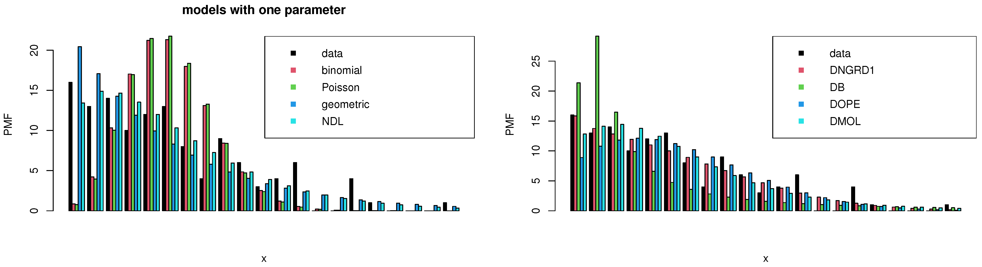
Based on the first and second datasets, the DNGRD probability model is contrasted and compared with the other seven competing models to show the reliability and superiority of the proposed model, including Poisson, binomial, geometric, discrete Burr (DB) by [37], discrete Marshall–Olkin Lomax (DMOL) by [38], new discrete Lindley (NDL) by [39], and discrete odd perks exponential (DOPE) by [40] distributions. To specify the best model, several criteria are used, namely: Akaike ( A I C = 2 p 2 l ^ ) , where p is the length of the model parameter and l ^ is log-likelihood value, consistent Akaike ( C A I C = 2 l ^ + 2 n p n p 1 ) , Bayesian ( B I C = 2 l ^ + p ln ( n ) ) , and Hannan–Quinn ( H Q I C = 2 l ^ + p ln ( ln ( n ) ) information criteria. Along with these, the X 2 s q u a r e statistic and its p-value are taken into account. If a probability model distribution has the highest p-value and the lowest values for all other metrics, it is obvious that it will provide the best fit for a particular collection of data. The maximum likelihood estimates (with their standard errors (St.Es)), as well as the fitted model selection criteria, are shown in Table 5 and Table 6 using the R programming language and the ’bbmle’ package in R program with version number (4.3.0), that was recommended.
To compare the performance and efficiency of the DNGR distribution with other distributions listed in Table 5, using measures of goodness of fit and p-values, we can proceed as follows:
1-DNGR versus DOPE:
DNGR shows a better fit with a lower A I C , C A I C , B I C , and H Q I C . The chi-squared value is lower for DNGR, indicating a better fit. DNGR has a higher p-value, suggesting a better fit to the data than DOPE.
2-DNGR versus Binomial/Poisson:
DNGR has a higher p-value than both binomial and Poisson distributions, indicating a more suitable model for the data. The information criteria (AIC, CAIC, HQIC) for DNGR are lower compared to binomial and Poisson, suggesting a better fit than binomial and Poisson.
3-DNGR versus DMOL:
DNGR and DMOL have comparable p-values, but DNGR shows better performance in terms of information criteria.
4-DNGR versus DB:
DNGR has a higher p-value than DB, indicating that DNGR shows slightly better performance in terms of information criteria.
5-DNGR versus Geometric/NDL:
DNGR outperforms both geometric and NDL distributions in terms of p-value, indicating a significantly better fit. DNGR has lower information criteria values, further suggesting its superiority in model fitting. Overall, DNGR appears to offer a more efficient and suitable fit for Data I compared to the other listed distributions.
Figure 3, Figure 4 and Figure 5 confirm these results for Data I (the black point refer to data; the pink point refer to DNGR distribution). Additionally, it is evident from Data II in Table 6 that the DNGR distribution is the best distribution among all the examined models in terms of the P-value, whereas Figure 6, Figure 7 and Figure 8 confirm these results for Data II. 
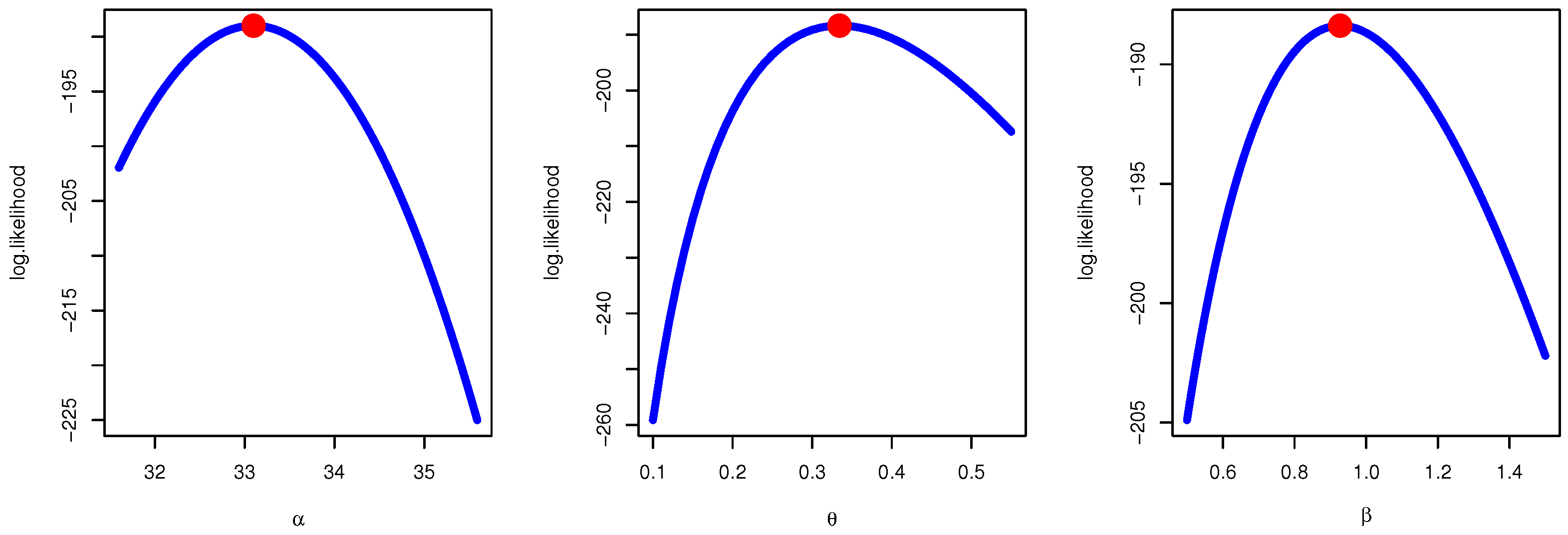
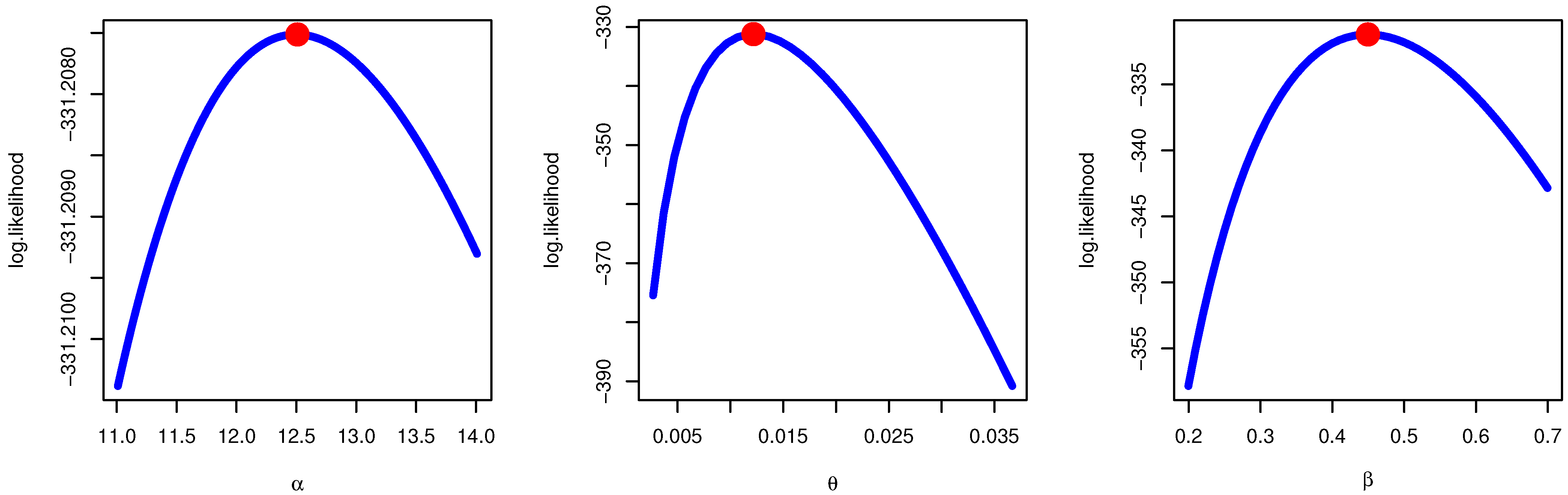
Figure 3 confirms the results of MLE fitting and demonstrates the existence, uniqueness, and maximum point of likelihood value of the likelihood estimates for Data I. 
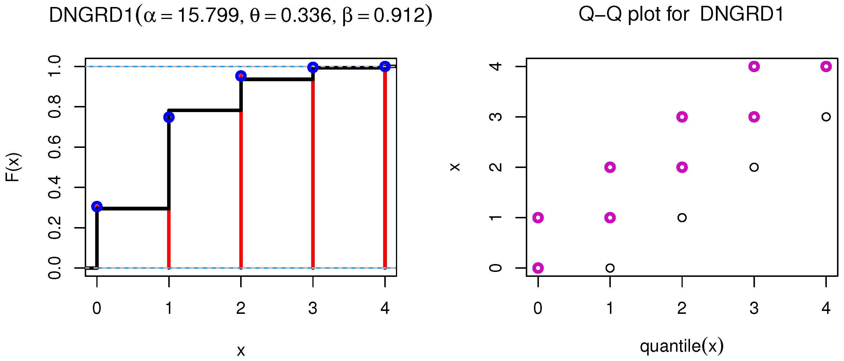
Figure 4 regarding associated empirical CDF and estimated CDF plot illustrates the connection between observed cumulative probability and observation through a visual plot and also Q–Q plot for Data I. Figure 5 highlights estimated frequency by using PMF for each comparative model for Data I. Table 7 indicates survival and hazard rate functions for DNGR distribution with different values of Data I, noting that the survival value decreased when the values of Data I increased, while the hazard rate value increased when the values x of Data I increased.
Figure 6 confirms the results of MLE fitting and demonstrates the existence, uniqueness, and maximum point of likelihood value of the likelihood estimates for Data II. Figure 7 regarding associated empirical CDF and estimated CDF plot illustrates the connection between observed cumulative probability and observation through a visual plot and Q–Q plot for Data II. Figure 8 highlights estimated frequency by using PMF for each comparative model for Data II. Table 8 indicates survival and hazard rate functions for DNGR distribution with different values of Data II, noting that the survival values decreased when the values of Data II increased, while the hazard rate value increased when the values x of Data II increased.

7. Conclusions

In this study, the authors successfully developed a novel discrete analog from the continuous generalized Rayleigh distribution denoted by DNGR through the application of the survival discretization method. Several key attributes of the DNGR model were studied, such as its unimodal probability mass function, which exhibits varying degrees of symmetry and skewness based on parameter selection. Comprehensive statistical measures for DNGR were derived, including moments, stress–strength function, moment-generating function, and mean residual and mean past lifetimes. The potential submodels and special cases derived from the DNGR demonstrate the versatility and adaptability of the DNGR distribution, which can be suitable for modeling different types of data and could provide unique insights depending on the context of the analysis. Furthermore, the practical applicability of the work was enhanced by conducting detailed simulation analyses and presenting the results in tabular form. Point and interval estimation using both the maximum likelihood and the Bayesian methods were obtained, supplementing these with simulation analyses executed using R code. This was complemented by a numerical analysis aimed at evaluating the estimation methods for DNGR’s unknown parameters and assessing the efficiency of these methods. A significant aspect of their contribution is the application of the DNGR model to real-world data. Two real data examples were selected, one from the industrial sector concerning UK coal mining strikes and another focusing on environmental issues related to fires in Greece. Their analysis revealed that the DNGR model outperformed seven competitive discrete distributions in various goodness-of-fit measures, demonstrating its superior ability to model the given datasets effectively. This finding was further illustrated through detailed tables and figures showcasing the properties and efficiency of the new model. As a pathway for future work, the authors suggest exploring alternative discretization methods to assess their performance and applicability to a broader range of real-life data scenarios.

Author Contributions

Conceptualization, H.H.A.; Methodology, H.H.A. and D.A.R.; Software, E.M.A.; Validation, D.A.R.; Formal analysis, H.H.A., E.M.A. and D.A.R.; Investigation, H.H.A. and E.M.A.; Resources, E.M.A.; Data curation, E.M.A.; Writing—original draft, H.H.A., D.A.R. and E.M.A.; Writing—review & editing, D.A.R. and H.H.A.; Funding acquisition, H.H.A. All authors have read and agreed to the published version of the manuscript.

Funding

This work was supported by the Deanship of Scientific Research, Vice Presidency for Graduate Studies and Scientific Research, King Faisal University, Saudi Arabia [GRANT No. 5476].

Data Availability Statement

Data are contained within the article.

Acknowledgments

This work was supported by the Deanship of Scientific Research, Vice Presidency for Graduate Studies and Scientific Research, King Faisal University, Saudi Arabia [GRANT No. 5476].

Conflicts of Interest

The authors declare no conflicts of interest.

References

  1. Xekalaki, E. Hazard function and life distributions in discrete time. Commun. Stat. Theory Methods 1983, 12, 2503–2509. [Google Scholar] [CrossRef]
  2. Hitha, N.; Nair, U.N. Characterization of some discrete models by properties of residual life function. Calcutta Stat. Assoc. Bull. 1989, 38, 219–223. [Google Scholar] [CrossRef]
  3. Roy, D.; Gupta, R.P. Classifications of discrete lives. Microelectron. Reliab. 1992, 32, 459–1473. [Google Scholar] [CrossRef]
  4. Roy, D.; Gupta, R.P. Stochastic modeling through reliability measures in the discrete case. Stat. Probab. Lett. 1999, 43, 197–206. [Google Scholar] [CrossRef]
  5. Roy, D. On classifications of multivariate life distributions in the discrete set-up. Microelectron. Reliab. 1997, 37, 361–366. [Google Scholar] [CrossRef]
  6. Roy, D. The discrete normal distribution, Commun. Stat. Theor. Methods 2003, 32, 1871–1883. [Google Scholar] [CrossRef]
  7. Roy, D. Discrete Rayleigh distribution. IEEE. Trans. Reliab. 2004, 53, 255–260. [Google Scholar] [CrossRef]
  8. Roy, D.; Ghosh, T. A new discretization approach with application in reliability estimation. IEEE. Trans. Reliab. 2009, 58, 456–461. [Google Scholar] [CrossRef]
  9. Lai, C.-D. Constructions and applications of lifetime distributions. Appl. Stoch. Model. Bus. Ind. 2013, 29, 127–140. [Google Scholar] [CrossRef]
  10. Lai, C.D. Issues concerning constructions of discrete lifetime models. Qual. Technol. Quant. Manag. 2013, 10, 251–262. [Google Scholar] [CrossRef]
  11. Ahmad, H.H.; Almetwally, E.M. Generating optimal discrete analogue of the generalized Pareto distribution under Bayesian inference with application. Symmetry 2022, 14, 1457. [Google Scholar] [CrossRef]
  12. Bracquemond, C.; Gaudoin, O. A survey on discrete life time distributions. Int. J. Reliabil. Qual. Saf. Eng. 2003, 10, 69–98. [Google Scholar] [CrossRef]
  13. Chakraborty, S. Generating discrete analogues of continuous probability distributions-A survey of methods and constructions. J. Stat. Distrib. Appl. 2015, 2, 6. [Google Scholar] [CrossRef]
  14. Al-Huniti, A.A.; Al-Dayjan, G.R. Discrete Burr type III distribution. Am. J. Math. Stat. 2012, 2, 145–152. [Google Scholar] [CrossRef]
  15. Bebbington, M.; Lai, C.D.; Wellington, M.; Zitikis, R. The discrete additive Weibull distribution: A bathtub-shaped hazard for discontinuous failure data. Reliab. Eng. Syst. Saf. 2012, 106, 37–44. [Google Scholar] [CrossRef]
  16. Yari, G.; Tondpour, Z. Discrete Burr XII-Gamma Distributions: Properties and Parameter Estimations. Iran J. Sci. Technol. Trans. Sci. 2018, 42, 2237–2249. [Google Scholar] [CrossRef]
  17. Eliwa, M.S.; Altun, E.; El-Dawoody, M.; El-Morshedy, M. A new three-parameter discrete distribution with associated INAR(1) process and applications. IEEE Access 2020, 8, 91150–91162. [Google Scholar] [CrossRef]
  18. Eldeeb, A.; Haq, M.A.U.; Babar, A. A Discrete Analog of Inverted Topp-Leone Distribution: Properties, Estimation and Applications. Int. J. Anal. Appl. 2021, 19, 695–708. [Google Scholar]
  19. Ahmad, H.H.; Almetwally, E. On discrete generalization of the inverse exponential distribution: Properties, characterizations and applications. AIP Conf. Proc. 2023, 2738, 020001. [Google Scholar] [CrossRef]
  20. El-Dawoody, M.; Eliwa, M.S. Bivariate Discrete Burr Lifetime Distribution: A Mathematical and Statistical Framework for Modeling Medical and Engineering Data. Inf. Sci. Lett. 2023, 12, 3199–3214. [Google Scholar]
  21. El-Dawoody, M.; Eliwa, M.S.; El-Morshedy, M. An Extension of the Poisson Distribution: Features and Application for Medical Data Modeling. Processes 2023, 11, 1195. [Google Scholar] [CrossRef]
  22. Al-Bossly, A.; Eliwa, M.S.; Ahsan-Ul-Haq, M.; El-morshedy, M. Discrete Logistic Exponential Distribution with Application. Stat. Optim. Inf. Comput. 2023, 11, 629–639. [Google Scholar] [CrossRef]
  23. Abd EL-Hady, A.E.; Hegazy, M.A.; EL-Helbawy, A.A. Discrete Exponentiated Generalized Family of Distributions. Comput. J. Math. Stat. Sci. 2023, 2, 303–327. [Google Scholar] [CrossRef]
  24. Rosaiah, K.; Kantam, R.R.L. Acceptance sampling based on the inverse Rayleigh distribution. Econ. Qual. Control 2005, 20, 277–286. [Google Scholar] [CrossRef]
  25. Merovci, F. Transmuted rayleigh distribution. Aust. J. Stat. 2013, 42, 21–31. [Google Scholar] [CrossRef]
  26. Cordeiro, G.M.; Cristino, C.T.; Hashimoto, E.M.; Ortega, E.M. The beta generalized Rayleigh distribution with applications to lifetime data. Stat. Pap. 2013, 54, 133–161. [Google Scholar] [CrossRef]
  27. Ahmad, A.; Ahmad, S.P.; Ahmed, A. Transmuted inverse Rayleigh distribution: A generalization of the inverse Rayleigh distribution. Math. Theory Model 2014, 4, 90–98. [Google Scholar]
  28. Gomes, A.E.; da-Silva, C.Q.; Cordeiro, G.M.; Ortega, E.M. A new lifetime model: The Kumaraswamy generalized Rayleigh distribution. J. Stat. Comput. Simul. 2014, 84, 290–309. [Google Scholar] [CrossRef]
  29. Nofal, Z.M.; Abd El Hadi, N.E. Exponentiated transmuted generalized Raleigh distribution: A new four-parameter Rayleigh distribution. Pak. J. Stat. Oper. Res. 2015, 11, 115–134. [Google Scholar]
  30. Iriarte, Y.A.; Vilca, F.; Varela, H.; Gomez, H.W. Slashed generalized Rayleigh distribution. Commun. Stat.-Theory Methods 2017, 46, 4686–4699. [Google Scholar] [CrossRef]
  31. Haj Ahmad, H.; Bdair, O.M.; Naser, M.F.M.; Asgharzadeh, A. The rayleigh lindley distribution: A new generalization of rayleigh distribution with physical applications. Rev. Investig. Oper. 2023, 44, 1–18. [Google Scholar]
  32. Shen, Z.; Alrumayh, A.; Ahmad, Z.; Abu-Shanab, R.; Al-Mutairi, M.; Aldallal, R. A new generalized Rayleigh distribution with analysis to big data of an online community. Alex. Eng. J. 2022, 61, 11523–11535. [Google Scholar] [CrossRef]
  33. Goliforushani, S.; Asadi, M. On the discrete mean past lifetime. Metrika 2008, 68, 209–217. [Google Scholar] [CrossRef]
  34. Kendall, M.G. Natural law in social sciences. J. R. Stat. Soc. Ser. 1961, 124, 1–19. [Google Scholar] [CrossRef]
  35. Ridout, M.S.; Besbeas, P. An empirical model for under dispersed count data. Stat. Model. 2004, 4, 77–89. [Google Scholar] [CrossRef]
  36. Karlis, D.; Xekalaki, E.; Lipitakis, E.A. On some discrete valued time series models based on mixtures and thinning. In Proceedings of the Fifth Hellenic-European Conference on Computer Mathematics and Its Applications, Athens, Greece, 20–22 September 2001; pp. 872–877. [Google Scholar]
  37. Krishna, H.; Pundir, P.S. Discrete Burr and discrete Pareto distributions. Stat. Methodol. 2009, 6, 177–188. [Google Scholar] [CrossRef]
  38. Ibrahim, G.M.; Almetwally, E.M. Discrete marshall–olkin lomax distribution application of COVID-19. Biomed. J. Sci. Tech. Res. 2021, 32, 25381–25390. [Google Scholar]
  39. Al-Babtain, A.A.; Ahmed, A.H.N.; Afify, A.Z. A new discrete analog of the continuous Lindley distribution, with reliability applications. Entropy 2020, 22, 603. [Google Scholar] [CrossRef]
  40. Elbatal, I.; Alotaibi, N.; Almetwally, E.M.; Alyami, S.A.; Elgarhy, M. On odd perks-G class of distributions: Properties, regression model, discretization, Bayesian and non-Bayesian estimation, and applications. Symmetry 2022, 14, 883. [Google Scholar] [CrossRef]
Figure 1. The pmf bar charts for the DNGR, (a) when α = 2 , (b) when β = 2 , and (c) when θ = 1 .
Mathematics 12 00183 g001aMathematics 12 00183 g001b
Figure 2. The HRF of the DNGR distribution.
Mathematics 12 00183 g002
Figure 3. Likelihood profile (blue line) with the maximum likelihood estimation (red dot): Data I.
Mathematics 12 00183 g003
Figure 4. Estimated CDF and Q–Q plot of DNGR by using MLE: Data I.
Mathematics 12 00183 g004
Figure 5. Estimated PMF of each comparative model by using MLE: Data I.
Mathematics 12 00183 g005
Figure 6. Estimated CDF and Q–Q plot of DNGR by using MLE: Data II.
Mathematics 12 00183 g006
Figure 7. Estimated PMF of each comparative model by using MLE: Data II.
Mathematics 12 00183 g007
Figure 8. Likelihood profile (blue line) with the maximum likelihood estimation (red dot): Data II.
Mathematics 12 00183 g008
Table 1. Summary of descriptive statistics for the DNGR distribution.
θ α β MinimumMeanVarianceMaximumSKKt
0.81.050.301.51400.46433−0.07001.2956
1.051.201.97600.33384−0.05631.3066
1.052.502.18900.31764−0.04791.3039
1.05312.24200.31374−0.04611.3030
2.20.300.64800.430530.12451.1141
2.21.201.24700.366430.02291.2125
2.22.501.53300.325230.02031.2296
2.2301.60200.317930.02121.2320
30.300.58100.409830.16291.1205
31.201.18800.357030.03731.2097
32.501.47700.317830.03201.2281
3301.54500.316330.03251.2307
1.51.050.301.08000.27993−0.06991.2957
1.051.201.46000.28273−0.05641.3066
1.052.501.65700.23963−0.04811.3039
1.05301.70200.22143−0.04611.3031
2.20.300.45200.286020.12441.1142
2.21.200.92100.219020.02291.2125
2.22.501.11200.161620.02031.2295
2.2301.15100.162420.02131.2321
30.300.40100.272520.16291.1205
31.200.88000.225820.03741.2096
32.501.08300.150320.03211.2280
3301.12100.148520.03251.2306
31.050.300.82300.15982−0.07001.2956
1.051.200.98900.06892−0.05631.3067
1.052.501.04600.06802−0.04801.3040
1.05301.06100.07342−0.04591.3031
2.20.300.28000.203820.12451.1143
2.21.200.68200.223120.02291.2123
2.22.500.88400.112720.02031.2296
2.2300.92000.085720.02101.2320
30.300.24200.185620.16281.1204
31.200.63600.235720.03741.2097
32.500.85900.129220.03211.2280
3300.90200.098520.03251.2307
Table 2. MLE and Bayes for parameters of DNGR distribution: α = 1.5 .
α = 1.5 MLEBayesian
θ β n RBMSELowerUpperCPRBMSELowerUpper
0.80.530 α 0.35871.52430.27604.836296.4%−0.06370.17961.16981.6971
θ 0.11630.30280.32781.458394.8%−0.09000.10960.56570.8743
β 2.84141.62170.38643.454997.4%0.27620.18460.42480.8864
70 α 0.14901.49330.37164.818696.2%−0.10360.20051.14241.5800
θ 0.01500.18980.44031.183794.0%−0.05720.06510.65860.8455
β 1.44251.58620.82673.615796.0%0.36450.21510.46090.9003
100 α 0.26701.28670.49874.299696.6%−0.07490.14731.20811.5686
θ 0.01410.13230.55271.069894.8%−0.05730.05560.68890.8096
β 0.92871.07450.99393.293596.2%0.29630.16360.51650.7786
200 α 0.25721.03810.59764.074393.4%−0.04330.08031.33031.5184
θ −0.04010.10440.57300.962995.0%−0.04460.04000.72570.7991
β 0.80440.91011.40053.643693.2%0.17730.09550.52220.6549
0.8230 α −0.26300.49480.51941.691796.4%−0.07230.18171.12061.6439
θ 0.19640.25330.56741.346995.0%−0.16270.15040.53600.8156
β 0.18210.61691.38753.341095.4%0.01930.15751.73502.3384
70 α −0.28760.46970.70421.432998.2%−0.06500.17821.14071.6102
θ 0.17810.20570.65141.233695.4%−0.14520.12840.58980.8055
β 0.17830.60751.39073.265897.6%0.02680.14011.80492.2871
100 α −0.23440.45310.84321.481099.8%−0.08670.16181.18621.5461
θ 0.18990.19680.70661.197395.4%−0.13170.11150.61740.7637
β 0.15850.54141.45613.178096.6%0.02430.09451.89412.2078
200 α −0.21440.38220.85231.470399.6%−0.04180.07961.34681.5366
θ 0.16310.15400.76991.091094.8%−0.11280.09310.66380.7529
β 0.14030.54021.37093.019098.4%0.01330.04821.94542.0992
1.30.530 α −0.01611.83750.12895.080695.2%−0.08930.20221.11911.6715
θ 0.24170.55740.71082.517697.0%−0.07700.16710.96491.5162
β 2.99861.96560.14954.493295.4%0.29960.19730.40970.8957
70 α −0.01271.80930.25494.917396.0%−0.12160.22071.13611.5891
θ 0.20730.46500.82612.313096.8%−0.07160.12431.05731.3653
β 1.02031.84240.23294.297096.0%0.40090.22950.47690.9082
100 α −0.01571.27600.29633.514795.8%−0.09730.17431.18481.5360
θ 0.17640.43090.85142.245097.2%−0.06250.10351.09521.3359
β 0.92560.96780.56123.817396.2%0.33400.18210.52920.8175
200 α −0.01420.92940.31713.060496.4%−0.05070.09121.33141.5228
θ 0.08130.31530.82281.988698.0%−0.03780.05941.19151.3146
β 0.56710.63150.62493.081699.2%0.19310.10290.52860.6659
230 α −0.31130.65510.13151.934799.4%−0.10120.21851.09861.6487
θ 0.15340.30041.05851.940393.6%−0.13060.20700.92521.3786
β 0.13340.74660.89863.634998.4%0.02350.15701.74582.3302
70 α −0.31170.65550.13101.933899.4%−0.10270.21851.09861.6487
θ 0.15260.29341.07441.922593.8%−0.12630.20670.92651.3857
β 0.13230.74380.90073.602898.4%0.02160.15291.75482.3035
100 α −0.32070.48111.00571.032193.8%−0.09140.21081.19021.4334
θ 0.19290.27561.31921.7823100.0%−0.11510.16561.01481.2705
β 0.08870.17761.91622.1927100.0%0.01540.07571.93162.1534
200 α −0.31880.47821.00961.034193.3%−0.05380.09461.32351.5159
θ 0.15940.24031.36821.746294.7%−0.07630.10431.14271.2673
β 0.08090.16831.92582.182195.9%0.01400.04961.95822.1127
Table 3. MLE and Bayes for parameters of DNGR distribution: α = 3 .
α = 3 MLEBayesian
θ β RBMSELowerUpperCPRBMSELowerUpper
1.30.530 α 0.19172.01850.22107.371296.2%−0.00380.15582.66893.2541
θ 0.53251.06760.39773.586893.2%−0.06960.16210.94861.4541
β 9.33885.03891.45368.885296.4%0.40230.22770.50100.8988
70 α 0.37361.80151.35376.887892.6%−0.00710.13132.73843.2252
θ 0.35980.63990.91102.624595.2%−0.07840.13001.04461.3579
β 9.75205.40790.78739.964896.4%0.55960.29290.60810.9368
100 α 0.30832.08380.26127.588495.4%−0.00400.08972.80733.1475
θ 0.35100.58471.03902.473596.2%−0.06270.10031.10331.3265
β 9.71695.47980.385710.331293.6%0.41140.21450.57990.8143
200 α 0.81183.56890.317310.553695.8%−0.00210.04522.90923.0800
θ 0.32230.47851.26552.172595.8%−0.03670.05851.17951.3146
β 9.65845.07712.25488.403696.0%0.23810.12410.55480.6959
0.930 α −0.15031.63600.53645.634995.6%−0.00380.16182.69923.3379
θ 0.37520.83570.45653.119197.8%−0.11040.19340.91101.3977
β 6.16476.25020.80195.094597.0%0.14880.18880.78051.3184
70 α −0.15841.08980.60064.449297.6%−0.01340.13952.70343.2184
θ 0.18300.44430.80172.274093.0%−0.11190.16940.97171.2952
β 5.35075.06492.63694.794497.8%0.12220.17220.89921.2938
100 α 0.13172.03700.65254.315694.2%−0.00310.08832.82463.1589
θ 0.21200.43310.92002.231192.0%−0.09010.13131.06291.2857
β 6.42286.03943.24864.112496.4%0.16330.16530.89641.1761
200 α 0.17011.69290.34363.677294.2%−0.00310.04612.89613.0742
θ 0.15680.26951.15781.849895.0%−0.04850.07041.18001.3009
β 6.76956.34413.52243.846397.2%0.08360.08480.90101.0514
20.530 α −0.18810.69571.63753.233895.6%−0.00470.15512.67213.2679
θ −0.04110.50580.93862.896990.0%−0.05530.19591.57652.2175
β 4.51802.51990.56834.949796.8%0.29920.19830.39970.9025
70 α −0.21160.82531.33053.3996100.0%−0.00670.13552.69833.2384
θ −0.06490.66390.59293.147597.2%−0.07260.18691.64642.0764
β 4.16152.39450.25584.9057100.0%0.46750.25630.51290.9282
100 α −0.21050.88251.15883.5784100.0%−0.00390.09292.82183.1785
θ −0.08370.65760.58493.0803100.0%−0.05650.13821.73562.0397
β 3.85752.23780.20234.6552100.0%0.31670.17230.53490.7985
200 α −0.07470.36072.22143.330392.6%−0.00210.04502.91623.0799
θ −0.21740.57740.81992.310595.2%−0.02750.06951.85802.0248
β 3.08231.76030.37253.709895.4%0.18030.09750.50840.6579
1.130 α −0.40951.46780.19573.347099.6%−0.00730.16202.68153.2895
θ −0.01050.68700.63193.3262100.0%−0.09110.23971.51402.1195
β 2.59313.52940.12578.030699.6%0.10340.18810.92281.5108
70 α −0.32891.18190.73683.2901100.0%−0.01270.14242.68253.1929
θ −0.10040.67820.52833.0700100.0%−0.09410.22111.57551.9901
β 2.37662.79791.75845.670197.8%0.16440.21401.05521.4943
100 α −0.27760.97881.15783.176992.8%−0.00750.08922.82123.1590
θ −0.17420.66670.53622.767193.0%−0.06550.15491.70242.0002
β 2.35822.79761.63835.749798.2%0.11110.14511.04701.3534
200 α −0.24450.82341.53203.001393.8%−0.00410.04532.89663.0706
θ −0.24360.56530.95042.075097.4%−0.03670.08441.85202.0008
β 2.24352.54272.36634.769496.6%0.05690.07531.08501.2456
Table 4. Data I: The number of strikes and their frequency that occurred in the UK coal mining industry.
data01234 or more
Freq46762491
Table 5. MLE estimates and different measures of fit for Data I.
EstimatorsSEAICCAICBICHQIC X 2 p-Value
DNGR α 33.099613.6357382.7571382.9150391.9067386.47333.67210.4522
θ 0.33430.0434
β 0.92760.1425
DOPE α 39.35843.5957387.5354387.6933396.6850391.25165.23730.2638
θ 0.27570.0264
β 3.13070.5099
Binomial θ 0.99370.1315386.1302386.1562389.1801387.368910.10780.0387
Poision θ 0.99360.0798386.1302386.1562389.1801387.36899.89860.0422
DB α 4.65240.6986388.4190388.4974394.5187390.89645.40760.2480
β 0.59400.0448
DMOL α 21.19607.5845386.4288386.5867395.5784390.14503.97710.4091
θ 1.88920.3088
β 0.00280.0009
Geometric θ 0.50170.0284433.1343433.1603436.1842434.373150.79840.0000
NDL θ 0.50170.0284433.1343433.1603436.1842434.373150.79840.0000
Table 6. MLE estimates and different measures for Data II.
EstimatorsSEAICCAICBICHQIC X 2 p-Value
DNGRD α 12.50912.5308668.4150668.6150676.8759671.852022.80250.2986
θ 0.01220.0027
β 0.44950.1299
DOPE α 44.21119.3605685.1374685.3374693.5983688.574432.63300.0370
θ 0.01340.0017
β 0.72910.0844
Binomial θ 0.96080.2622821.7835821.8163824.6038822.929212776.33870.0000
Poision θ 5.06450.2021821.7835821.8163824.6038822.929226469.54650.0000
DB α 2.53850.4910748.2257748.3249753.8663750.517091.35360.0000
β 0.76110.0425
DMOL α 4.63491.8610674.2602674.4602682.7210677.697225.00950.2011
θ 13.01803.2683
β 0.00310.0018
Geometric θ 0.16490.0135675.3352675.3679678.1554676.480827.51520.1214
NDL θ 0.16490.0135675.3352675.3679678.1554676.480827.51520.1214
Table 7. Survival and hazard rate functions for DNGR distribution with different values of Data I.
x S x ; 33.0994 , 0.3343 , 0.9275 h x ; 33.0994 , 0.3343 , 0.9275
00.69520.4383
10.25181.7607
20.04724.3343
30.00459.3889
40.000219.2691
Table 8. Survival and hazard rate functions for DNGR distribution with different values of Data II.
x S x ; 12.5091 , 0.0122 , 0.4495 h x ; 12.5091 , 0.0122 , 0.4495
00.87210.1466
20.65770.1572
40.47250.1879
50.39190.2059
80.20230.2686
200.00230.6490
Disclaimer/Publisher’s Note: The statements, opinions and data contained in all publications are solely those of the individual author(s) and contributor(s) and not of MDPI and/or the editor(s). MDPI and/or the editor(s) disclaim responsibility for any injury to people or property resulting from any ideas, methods, instructions or products referred to in the content.

