Abstract
Alzheimer’s disease (AD) affects about a tenth of the population aged over 65 and nearly half of those over 85, and the number of AD patients continues to grow. Several studies have shown that the variant of the apolipoprotein E () gene is potentially associated with an increased risk of AD. In this study, we aimed to investigate the causal effect of - on Alzheimer’s disease under the potential outcome framework and evaluate the individualized risk of disease onset for - carriers. A total of 1705 Hispanic individuals from the Washington Heights-Inwood Columbia Aging Project (WHICAP) were included in this study, comprising 453 - carriers and 1252 non-carriers. Among them, 265 subjects had developed AD (23.2%). The non-parametric Bayesian additive regression trees (BART) approach was applied to model the individualized causal effects of - on disease onset in the presence of right-censored outcomes. The heterogeneous risk of - on AD was examined through the individualized posterior survival probability and posterior causal effects. The results showed that, on average, patients carrying - were years younger at onset than those with non-carrying status, and the disease risk associated with - carrying status was higher than that for non-carrying status; however, it should be noted that neither result was statistically significant. The posterior causal effects of - for individualized subjects indicate that 14.41% of carriers presented strong evidence of AD risk and approximately 38.65% presented mild evidence, while around 13.71% of non-carriers presented strong evidence of AD risk and 40.89% presented mild evidence. Furthermore, 79.26% of carriers exhibited a posterior probability of disease risk greater than 0.5. In conclusion, no significant causal effect of the - gene on AD was observed at the population level, but strong evidence of AD risk was identified in a sub-group of - carriers.
MSC:
62P10
1. Introduction
Alzheimer’s disease (AD) is a devastating neurological disease that affects millions of people around the world. About one in ten people over 65 and almost half of people over 85 suffer from AD [1], and the number of afflicted individuals continues to grow annually. It has been revealed that the apolipoprotein E locus () gene is associated with an increased risk of AD onset, in both sporadic and familial forms [2,3]. Particularly, among three alleles, the epsilon 4 (E4 or ) variant of has been found to be an important factor in the etiology of more than half of all AD [2,4]. Thus, determining how to quantify the risk of - on AD is critical. In previous studies, a research team from Duke University concluded that - was associated with AD as a major risk factor using the Mantel–Haenszel correlation statistic and Cox proportional hazard model [2]. Another study using logistic regression has also revealed that - was associated with a higher AD risk [4]. A meta-analysis showed that - was a major risk factor across ethnic groups, ages, and gender [5]. In addition, a twin study suggested that multiple susceptibility genes along with - contributed to around 80% of AD cases [6]. However, the above studies on the effects of the gene on AD were all based on statistical association analysis. So far, to the best of our knowledge, there have been very limited studies evaluating the risk of - on AD in terms of causal effect at individualized level [2,5,6]. Assessing the AD risk using the causal effect of - at the individual level could help to target patients who may be susceptible to - [7,8].
Treatment effects (or risk) of specific treatments or interventions are usually evaluated at population level in randomized controlled trial (RCT) studies. However, in practice, clinical decisions are often made at the individual level. Real-world observations include large amounts of clinical information about patients, hence offering us an opportunity to infer the treatment effects for heterogeneous patients, even from a causal perspective. It is well known that the causal effect of treatment can be inferred under the potential outcome framework by Rubin [9], which usually requires strong assumptions before performing causal inference. An advantage of the potential outcome framework is that it can be employed to infer the individualized treatment effect [10], for which the causal effect of a specific treatment can be identified under the assumption that treatment is independent of potential outcome of treatment and control, given the pre-treatment covariates. The individualized treatment effect (ITE) is an important measure that has been widely investigated in the field of personalized medicine [11], which helps to quantify individualized responses to specific treatments for heterogeneous individuals by calculating the difference of outcomes between treatment and control for any patient. A major challenge in the models of the ITE method is to handle the non-linear relationship between the covariates and survival outcomes, especially in the presence of complex censoring.
Bayesian additive regression trees (BART) is an ensemble learning method by which the value of any unknown function can be approximated through the summation of a series of Bayesian regression trees. In particular, BART is flexible, powerful, and can handle the complex non-linear relationships and interactions among covariates [12,13]. More importantly, the Bayesian framework allows for the construction of 95% credible intervals for statistical inference. In practice, BART applies to both continuous and binary outcomes; hence, it has a wide range of applications. It has also recently been generalized to survival analysis [14,15] and can handle right-censored data [16], even interval-censored data [17]. Furthermore, BART is suitable for observational studies [12]. Therefore, the BART method can also be used to estimate the ITE and conduct causal inference. Finally, BART can easily be extended to various settings, and a generalized BART model that unifies extensions is called general BART [18]. Generalized BART is commonly used for non-parametric or semi-parametric problems, correlated outcomes, survey matching problems, and models with weaker distributional assumption. The flexible extensibility of BART is a particular advantage in practical applications.
In this article, we aim to assess the causal risk of - on AD in the presence of right-censored observations under the potential outcome framework and examine the individualized risk of disease onset for - carriers. To the best of our knowledge, the data analysis in existing studies focused on AD has concluded merely in terms of the correlation, instead of the causal association between AD and -. The novelty of this article lies in the investigation of causal associations between - and AD using BART, a hybrid Bayesian and machine learning method, which enables us to estimate and infer the causal effect of interest at both the population and individual level. In particular, the key contributions of this paper are as follows:
- We apply the BART method to a non-parametric AFT model for right-censored data;
- We infer the causal effect of - on AD at both population and individual levels under the potential outcome framework;
- We explore heterogeneous evidence of the causal effect and identify important variables associated with the causal effect.
The remainder of this article is organized as follows. The data, notation, and statistical models are described in Section 2. In Section 3, we present the results regarding the estimated gene effect of - on AD with respect to age at onset and onset risk for each patient. We conclude with a brief discussion in Section 4.
2. Model and Methods
2.1. Notation
Suppose there are n patients in the study. For the patient, let denote the true AD onset time and denote the censoring time. Denote the observed AD onset time as and the censoring indicator as . Let be an indicator of carrying the - gene, such that indicates assignment to the treatment group and indicates assignment to the control group. Let denote a vector of baseline covariates. Therefore, the observed data can be denoted as . We make some regular assumptions for identifying the causal effect. First, the treatment assignment is strongly ignorable. Denote and as the potential outcomes under the treatment and the control , respectively. We assume that the treatment is independent of the potential outcome and , given . Furthermore, the treatment probabilities for the patients are bounded away from 0 and 1; that is, .
2.2. Non-parametric Accelerated Failure Time BART Model
To explore the causal effect of - on Alzheimer’s disease using a general and flexible model, we consider a non-parametric AFT model, defined as follows
where is modeled using a non-linear function and the residual term satisfies . In the following, we name (1) as the AFT-BART model.
For the model regression, we use Bayesian additive regression trees to approximate the unknown non-linear function . Let T denote a binary tree that consists of the tree structure and the interior node decision rules leading to subsequent nodes; in particular, all of the interior nodes of T have decision rules. Rules decide a pair to either the left or right node. Let be the parameter values (mean response of the subgroup of observations) associated with the b leaf nodes of the tree T. Given the tree model and a pair , we can define the value obtained at the leaf node and report the value associated with that leaf node. BART consists of two parts: A sum-of-trees model and a regularization prior. We denote the single tree model function as . The regression function m is represented in BART as a sum of the individual tree contributions
where each denotes a single tree model. Let be the set of all trees except for , and define similarly. The sum-of-tree model begins taking the fit from the first weak-learning tree, . After the fitting process, the model subtracts the first fit from the observed response and forms residuals. Then, the model fits the next tree to the residuals. The above procedure is performed m times in total. In the spirit of boosting, the number of trees in the model can be large, allowing each tree to contribute only a small part to the total fit. Over-fitting can be avoided through the use of a regularization prior, which limits the fit of each tree. The second piece of BART is the prior. In our analysis, we used the prior settings recommended for the AFT-BART model [14]. When using BART, the AFT model is fully non-parametric, and both the regression function and error distribution are modeled non-parametrically. The random error term follows a flexible location mixture of normal densities.
In essence, Algorithm 1 is an algorithm for the non-parametric AFT model in the presence of right-censored data, which is an extension of the BART model. In particular, it assumed to be a DP mixture model for the residual distribution. Under the non-parametric AFT framework, it deals with right censoring using a data augmentation technique with truncated normal distribution.
| Algorithm 1 Bayesian algorithm for the AFT-BART model. |
Input: Data , , initial values for , , , the on the residual, , and other parameters variables .
Output: New values of , , , and , . |
In AFT-BART, on f and on are treated as parameters in a formal statistical model. We used the prior settings recommended for AFT-BART [1]. After setting the prior on the parameters, the posterior can be computed using a Markov chain Monte Carlo (MCMC) technique; in particular, a Gibbs sampler was extended for computation of the posterior. After updating the trees and the terminal leaf node parameters, the parameters of the residual distribution can then be updated. The part of the residual distribution J can be expressed as
Here, the mixing distribution G is truncated to have a large, finite number of components H. for . We summarize the algorithm for this model as Algorithm 1. In the analysis, we set 5000 as the number of MCMC iterations to be treated as burn-in and 1000 as the number of iterations for posterior drawing. Furthermore, we set the number of trees as 200.
Base on the above models, we can estimate the individualized treatment effect (ITE), which can be expressed as the difference in expected log disease-onset time in the treatment group versus that in the control group. The ITE for a subject with covariate x can be calculated as
In this scenario, the ITE represents the difference in age at onset of AD for patients.
2.3. Onset Probability Analysis
Let the binary outcome of AD be Y, where denotes the onset endpoint of the participant and denotes the unobserved endpoint of the participant. It is straightforward to adapt or extend BART to the probit model. Define
where
and is the cumulative distribution function of standard normal distribution, denotes the binary regression tree, and denotes the associated terminal node parameters of tree j. Each probability is obtained as a function of . This idea differs from traditional aggregate classifier approaches, which often use a majority or average vote based on an ensemble of weak learners. For posterior calculation, the latent variables are introduced into the model [19], with if and if . Here, means independent and identically distributed. Finally, we obtain and . We summarize the BART method [12,20] in Algorithm 2.
| Algorithm 2 Bayesian back-fitting algorithm for updating BART |
Input: Data , , initial values for , , , and other parameters/variables .
Output: New values of , , . |
In the binary case, the ITE for a patient with covariate vector x can be defined as
In this scenario, the ITE represents the risk of onset of AD for a patient.
2.4. Posterior Inference Statistics
To predict the outcome Y for a particular x, we take the empirical average of the after burn-in sample , as follows:
The individual-level causal effects can be estimated as
Given the conditions on the X values in the sample, the conditional average treatment effect can be estimated as follows
We utilize the posterior probabilities of the differential treatment effect to detect the presence of heterogeneous treatment effects
along with the closely related quantity
Here, denotes the posterior probability that measures whether is greater than or equal to 0. For patient i, there exists a strong evidence of a differential treatment effect if ; that is, or . Mild evidence of a differential treatment effect exists if ; that is, or .
Another research line involves quantifying the heterogeneous treatment effects using the proportion of individuals who benefit from treatment. The proportion of benefit measure provides an interpretation and a useful quantity for determining the presence of cross-over or qualitative interactions among variables. The treatment effect in some cases may have the opposite sign, in comparison to the overall average treatment effect. A low proportion of patients benefiting in a situation where an overall treatment benefit has been determined may indicate the existence of cross-over interactions. With the treatment differences , we define the benefit proportion as
Here, Q is the posterior mean, which is the average of the posterior probabilities of treatment benefit . Treatment assignment for a patient can be decided according to the posterior probabilities of treatment benefit with or .
Based on the above, we summarize the methods for determining the continuous survival outcome and binary outcome in Algorithm 3. The corresponding R codes and a brief intrduction of the implementation are presented in Appendix A.
| Algorithm 3 Effect Estimation of - on AD |
Input: Two data sets in total, n training samples in each. , ; , .
Output: and CI of age at onset, and CI of onset risk, evidence for heterogeneity of treatment effect . |
3. Application
WHICAP is an ongoing community-based study of aging and dementia among elderly subjects residing in Northern Manhattan [21]. Proband participants were identified from Medicare records aged 65 years or older and recruited in 1992 and 1999. The prevalence of AD and dementia in proband participants was carefully monitored during the study. Dense genome-wide genotypes were collected in probands with more than two million SNPs. We focused on Hispanics, as they are one of the largest and fastest-growing ethnic groups in the United States [22]. They are generally under-studied, and the incidence of AD has been shown to increase by twofold in Hispanic elderly individuals, compared to white individuals [23]. Although WHICAP provides pedigree information and familial observations of probands, parents, and siblings, we only considered the probands in this study, as the genotypes in relatives of the proband were unobservable.
For this study, we enrolled 1705 probands of Alzheimer’s disease with observed AD onset time, where 453 (27%) were - carriers while 1252 (73%) were non-carriers. The characteristics of probands with AD onset time are summarized in Table 1. Furthermore, there were 1720 probands whose disease status (i.e., AD or not) was observable, where 458 participants were - carriers and 1262 were non-carriers. We also included three baseline covariates in the model: sex, educational attainment level, and race. The survival endpoint that we examined was the age at onset of patients (reported in years). We divided educational attainment into three levels (“<−0.9”, “−0.9∼0.5”, and “0.5 ∼ 2.0”). For the binary response model, we only included sex and educational attainment.

Table 1.
Characteristics of probands with Alzheimer’s disease for continuous age at onset.
3.1. Overall Causal Effect of Patients at Onset
We estimated the causal effect of - on Alzheimer’s disease using BART [24] and a BART-based accelerated failure time model. We also compared the AFT-BART method with other existing methods under the potential outcome framework. The first method involved the application of the AFT interaction model [17]. For our application, the ITE was calculated by subtracting the estimate under control assignment from the estimate under treatment assignment. Another related method used two separate AFT models: one for the treatment group and another one for the control group. The other method was based on a survival Causal Tree and Causal Forests. We built each survival Causal Tree using the function CausalTree in the R package SurvivalCausalTree [25].
The causal effects of - on Alzheimer’s disease, according to the models, are presented in Table 2. The analysis causal effect using AFT-BART indicated that the conditional average effect of the - gene on Alzheimer’s disease was in log years difference; that is, patients with the - gene presented 0.032 log years earlier age at onset than patients without -, on average. From the results using AFT-BART and BART to analyze the non-censored data, the age at onset was 0.001 and 0.003 log years earlier than those without -, respectively.
Table 2.
The causal effects of - on Alzheimer’s disease according to BART and BART-based accelerated failure time models (unit: log years).
The survival time posteriors for patients with and without - are presented in Figure 1. The red line is the posterior survival time of patients with -, while the black line is the posterior survival time of patients without -. It can be seen that the two lines do not overlap completely, which directly indicates that patients with - tend to present an earlier onset of Alzheimer’s disease, compared to those without -.
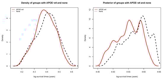
Figure 1.
(left) Density of survival time for groups with and without -; and (right) posterior of survival time for groups with and without -.
Table 3 presents the difference in AD onset risk associated to -. The results show that patients with the - gene have an onset risk of AD of 0.166, while those without - gene have an onset risk of AD of 0.127. Thus, the - gene increases the mean onset risk by 0.039 for patients with -, compared with those without it.
Table 3.
The estimated treatment effects of - on AD by BART for onset risk with 95% credible interval.
3.2. Distribution of Causal Effect for Patients
To characterize the variation in the causal effect of - on AD, we plotted the histogram and distribution of causal effect for patients, as presented in Figure 2. Smooth posterior estimates provide the causal effect distribution of - on Alzheimer’s disease for all patients. The histogram was constructed using all point estimates from both patients with and without the - gene. The blue part indicates the total treatment effect for patients with -, while the red part indicates the treatment effect for patients without -. Three peaks can be observed in the histogram, both for all patients and for the individual groups. The major patients with - presented an earlier age at onset than those without -: about 0.06 and 0.01 log years earlier at onset. However, a minority of patients presented opposite results. Among these patients, the patients with - had about 0.03 log years earlier time of AD onset than patients without -. It seems that these patients presented Alzheimer’s disease onset at a later age, or were affected by the existence of cross-over interactions. Overall, the majority of patients showed an earlier age of onset associated to -.
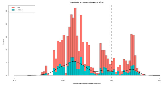
Figure 2.
Distribution of causal effect on -.
3.3. Individualized Treatment Effect
Figure 3 presents the individualized treatment effect estimates for the 1705 patients, clearly indicating an overall earlier age at onset associated to - for patients. The estimates consist of posterior means of treatment effect with corresponding credible intervals for all patients. There are two obvious groups of patients, according to the difference in onset time. The patients whose treatment effect was less than 0 had an earlier age at onset due to the - gene. It is clear that some patients had the treatment effect and credible intervals below zero. The causal effect of - on Alzheimer’s disease in these patients presented significant statistical significance. The variation in the treatment effects suggests substantial heterogeneity in response to -, which may be due to some individualized characteristics.
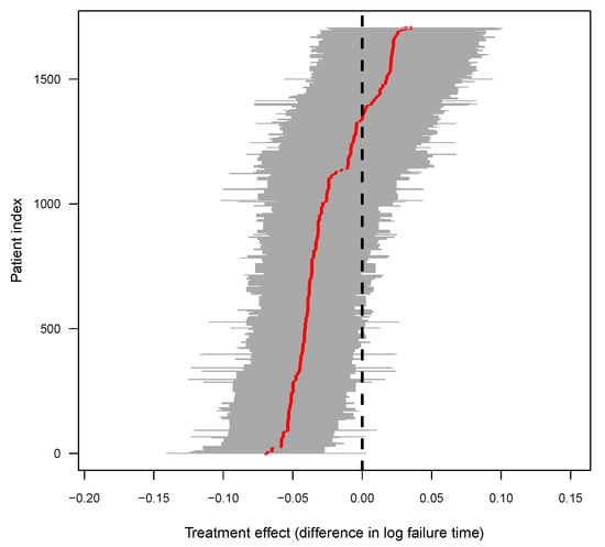
Figure 3.
Posterior of causal effect for individual patients, where the red line shows the posterior mean treatment effect for all of the patients, and the gray area show the 95% credible interval of each individualized - gene effect on AD.
The patients which presented a significant causal effect caused by - were extracted, for 515 patients in total. Table 4 presents the patients with and without significant ITE, grouped by sex, race, and education level. In particular, 171 patients were male and 344 were female; in terms of the education level of patients, 116 patients received education of low level, 259 patients received education of middle level, and 140 patients received high level education; as for race, the number of patients characterized by the four races were 138, 176, 191, and 10, respectively.
Table 4.
Patients with and without significant ITE, grouped by sex, race, and education level.
3.4. Covariate-Specific Treatment Effects
We constructed partial dependence plots for survival time (in years) of patients, along with the posterior distributions of treatment effect in male and female groups, each of the four races, and sub-groups defined according to educational attainment level. For the male and female groups, the posterior of survival time for male and female patients and difference in survival time between male and female patients are presented in Figure 4. The posterior of onset distribution and treatment effect in the male group were not distinct from those in the female group.
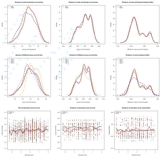
Figure 4.
(top-left) Density of survival time by sex; (top-middle) Posterior of survival time by sex; (top-right) Difference in survival time by sex; (mid-left) Density of survival time by race; (mid-middle) Posterior of survival time by race; (mid-right) Difference in survival time by race; (bottom-left) Density of survival time by education level; (bottom-middle) Posterior of survival time by education level; and (bottom-right) Difference in survival time by education level.
Next, we examined the four race groups of patients, and the posterior survival time and difference in survival time for the four groups are presented in Figure 4. The onset distributions and treatment effects in the first three race groups were highly similar, but distinct from those for the fourth race group. The possible explanation is that the sample size of fourth race group was very small (28 patients), and only accounted for .
Figure 4 presents the posterior of the survival time and difference in survival time for patients grouped by educational attainment level. The partial dependence plots clearly show differences between patients with and without - in the posterior distribution, except for a crossover point, where the sample size may have not been large enough. In the posterior of treatment effect, the median curves for both patients with and without - were below zero, clearly indicating the earlier age at onset caused by the - gene.
3.5. Individual Survival Curves
Figure 5 displays the individual posterior survival curves; in particular, there were 1705 individual survival curves associated to patients. The gray and black lines indicate the survival curves for patients with and without -, respectively. Although the survival curves of the two groups overlap to some extent, the patients without - had a higher survival proportion than those with -, overall. At the same age, the patients with - presented higher onset probability than those without -. The red and green lines are the posterior mean survival curves for patients with and without -, respectively; it can be seen that the red line lies above the green line. This indicates that patients with - are more likely to have an earlier onset of AD than those without -.
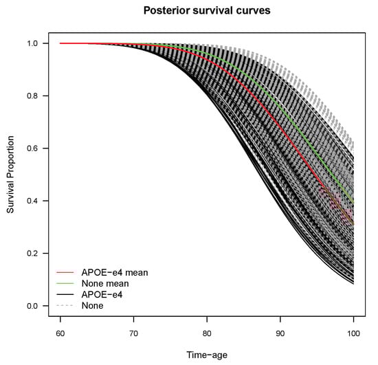
Figure 5.
Individual posterior survival curves for patients.
3.6. Evidence for Heterogeneous Treatment Effects
The posterior probabilities of treatment benefit are provided in Table 5. Table 5 shows that, among patients with -, 29.80% of patients presented strong evidence of a differential treatment effect, while approximately 54.97% of patients presented mild evidence. Among patients without -, approximately 30.35% of patients presented strong evidence of a differential treatment effect, while 56.39% presented mild evidence. For the proportion of patients who benefited from treatment, 77.93% of patients with - and 78.83% of patients exhibited a posterior probability of benefit greater than 0.5. These patients are more likely to have an earlier age at onset caused by the - gene.
Table 5.
Posterior probabilities of - carrier benefit and differential treatment effect among subjects with and without -.
Table 5 also shows that the probability of difference of onset among patients with and without -. Among patients with -, 14.41% of patients presented strong evidence of Alzheimer’s disease onset risk, while approximately 38.65% presented mild evidence. Among patients without -, approximately 13.71% of patients presented strong evidence of Alzheimer’s disease onset risk, while 40.89% presented mild evidence. Furthermore, posterior probabilities of treatment benefit can be used for treatment assignment for patients with or when estimating onset risk. It was found that 79.26% of patients with - and 82.57% of patients exhibited a posterior probability of benefit greater than 0.5. These patients are more likely to have higher onset risk caused by the - gene.
3.7. Important Factors
To explore important factors or features driving the differences in treatment effect, we proposed the use of BART to select important variables through identifying the most frequently used variables in the model. In this way, we may identify those predictors which have the most significant influence on the response. The number of trees was set as 50, and the frequencies of variables used are presented in Figure 6. The median used frequency of the sex variable was 20 and the 95% interval was [13,26]. The median used frequency of the education level variable was 24 and the 95% interval was [16,34]. Therefore, the education level variable is a more important predictor than the sex variable.
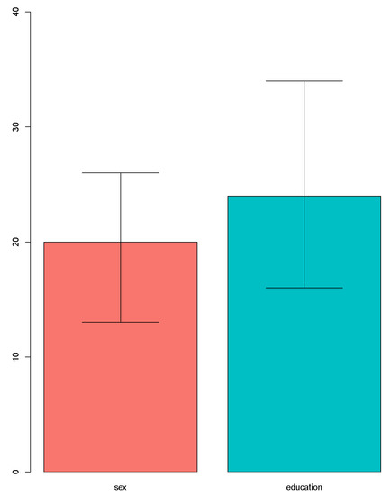
Figure 6.
The importance of variables using BART.
4. Discussion
In this study, we estimated the effect of the - gene on onset risk of AD at the individual level. The individualized effects were qualified by constructing a credible interval for every patient. In particular, in this way, the individualized effects for any patient and their credible interval can be inferred, instead of those at the population level. This may help to better target those patients who are more significantly affected by -. Furthermore, we can estimate the effects of - at the population level, based on the individualized effects. We inferred the effect of - on AD using causal inference. As such, assumptions for observational data were necessary, such as strong ignorability, which may induce treatment selection bias in the observational data. Further, in order to perform causal inference on observational data, the assumptions of overlap and no hidden confounders had to be made.
According to the causal effects for all patients, the causal effect of - on AD was not statistically significant at the population level. However, we observed a sub-population of patients presenting significant causal effects. Compared with the patients without significant causal effects, this sub-population had a higher proportion of female patients. Patients with low educational attainment level tended to present significant causal effects. In terms of the race of patients, patients of race 2 and race 3 in the sub-population accounted for higher proportions than in those without significant causal effects.
In the data analysis, we used BART to estimate the causal effects of - on AD for patients at the individual level. BART has been shown to be efficient and flexible, and has better or comparable performance to non-Bayesian competitors such as Boosting, LASSO, neural networks, and random forests [13]. BART has been shown to have good prediction performance and performs well for causal inference in various scenarios. Furthermore, it is necessary to quantify the outcome, especially in clinical research. In this context, Bayesian methods can provide natural credible intervals for outcomes. Although it is based on the potential outcome framework, our method may contribute to the identification of potential factors associated to the outcome at the causal level, which may help to determine the front node and directed path in the construction of the Bayesian network.
There are several metrics used for evaluation in this work. First, the prediction accuracy and the quantified uncertainty of prediction results are the most important metrics in clinical applications. In this line, we provided the estimate bias of the causal effect of - on AD and the 95% credible interval. As we handled right-censored data in this work, the effect of the censoring rate on the accuracy and efficiency of inference can be evaluated using Monte Carlo simulation techniques.
There were some limitations to our study; for example, there were no more than three baseline variables. We only included three variables and two variables for time-to-event data and binary outcome data, respectively. The inference for causal effects was limited by the few variables, as they only provided limited information. When analyzing data employing BART, as an MCMC technique, it can be computationally demanding; as such, the method was computationally expensive and required a significant amount of time for execution.
Author Contributions
Conceptualization, B.L.; methodology, Y.X. and B.L.; software, Y.X.; validation, Y.X. and B.L.; formal analysis, Y.X. and B.L.; investigation, B.L.; resources, B.L.; data curation, B.L.; writing—original draft preparation, Y.X.; writing—review and editing, B.L.; visualization, B.L.; supervision, B.L.; project administration, B.L.; funding acquisition, B.L. All authors have read and agreed to the published version of the manuscript.
Funding
This research was supported by the National Natural Science Foundation of China [11901013], Beijing Natural Science Foundation [1204031], Scientific Research and Development Funds of Peking University People’s Hospital [RDX2021-05], and the project 2020BD029 supported by PKU-Baidu Fund.
Informed Consent Statement
Not applicable, as this research uses a publicly available data set.
Data Availability Statement
The data presented in this study are available upon request from the corresponding author.
Conflicts of Interest
The authors declare no conflict of interest.
Appendix A. Implementation
The AFT-BART Model is a non-parametric Bayesian AFT model which combines a sum-of-trees model for the regression function and a DP mixture model for the residual distribution. This method was implemented based on the AFTrees package of the R software (version R-4.3.1).
To install and use the AFTrees package in R software, the development version of the package can be obtained from the GitHub website.The package can be installed directly from github, or downloaded and installed from the local files. For remote installation, the following commands should be run:
- install.packages("devtools")
- library(devtools)
- install_github("nchenderson/AFTrees")
First, we processed the data set and constructed the data frame for the model. The data consisted of n independent measurements . We split the data set into three folds and analyzed the data three times. Each time, two folds were used as the training set and the remaining fold was used as the testing set.
- library(caret)
- library(AFTrees)
- source("SurvivalProb-AD.R")
- # loading data ...
- set.seed(1)
- data <- read.csv(’AD_Data.csv’)
- censor_data <- data
- n <- nrow(censor_data)
- d <- 3
- X <- cbind(censor_data$X.1, censor_data$X.2, censor_data$X.3)
- # treatment indicators
- W <- censor_data$G_i
- Y <- censor_data$Y
- status <- censor_data$delta
- # prepare data
- colnames(X) <- colnames(X, do.NULL = FALSE, prefix = "x")
- AD_data <- data.frame(X, W = W, Y = Y, status = status)
- n <- nrow(AD_data)
- # data split
- set.seed(10)
- fold_idx <- createFolds(y = AD_data$W, k=3)
We split the data into training and testing sets, and used the Bayesian non-parametric AFT Model to estimate the conditional average treatment effect by employing BART. In BART, the number of trees was set as 200. In the MCMC iterations, we set 5000 iterations to be treated as burn-in and 1000 as the number for posterior drawing. The implementation details are as follows:
- for(i in 1:3){
- cat("\n NO.", i, "fold analysis ...\n")
- train_data <- AD_data[-fold_idx[[i]], ]
- est_data <- AD_data[fold_idx[[i]], ]
- # IndivAFT ...
- bart.tot <- IndivAFT(x.train = as.matrix(xtrain),
- y.train = train_data$Y,
- status = train_data$status,
- Trt = xtrain$W,
- x.test = as.matrix(xtest),
- ntree = 200,
- ndpost = 1000,
- nskip = 5000)
- ite <- colMeans(bart.tot$Theta.test)
- }
The posterior of individual treatment effects could then be obtained. The result was a matrix with posterior drawn times rows and test case size columns. In order to obtain the ITE posterior means, we averaged the output values in a column-wise manner.
References
- Evans, D.A.; Funkenstein, H.H.; Albert, M.S.; Scherr, P.A.; Cook, N.R.; Chown, M.J.; Hebert, L.E.; Hennekens, C.H.; Taylor, J.O. Prevalence of Alzheimer’s disease in a community population of older persons: Higher than previously reported. JAMA 1989, 262, 2551–2556. [Google Scholar] [CrossRef]
- Corder, E.H.; Saunders, A.M.; Strittmatter, W.J.; Schmechel, D.E.; Gaskell, P.C.; Small, G.W.; Roses, A.D.; Haines, J.L.; Pericak-Vance, M.A. Gene dose of apolipoprotein e type 4 allele and the risk of alzheimer’s disease in late onset families. Science 1993, 261, 921–923. [Google Scholar] [CrossRef] [PubMed]
- Ortega-Rojas, J.; Arboleda-Bustos, C.E.; Guerrero, E.; Neira, J.; Arboleda, H. Genetic Variants and Haplotypes of TOMM40, APOE, and APOC1 are Related to the Age of Onset of Late-onset Alzheimer Disease in a Colombian Population. Alzheimer Dis. Assoc. Disord. 2022, 36, 29–35. [Google Scholar] [CrossRef] [PubMed]
- Corder, E.H.; Saunders, A.M.; Risch, N.J.; Strittmatter, W.J.; Schmechel, D.E.; Gaskell, P.C., Jr.; Rimmler, J.B.; Locke, P.A.; Conneally, P.M.; Schmader, K.E.; et al. Protective effect of apolipoprotein E type 2 allele for late onset Alzheimer’ disease. Nat. Genet. 1994, 7, 180–184. [Google Scholar] [CrossRef] [PubMed]
- Farrer, L.A.; Cupples, L.A.; Haines, J.L.; Hyman, B.; Kukull, W.A.; Mayeux, R.; Myers, R.H.; Pericak-Vance, M.A.; Risch, N.; van Duijn, C.M. Effects of age, sex and ethnicity on the association between apolipoprotein E genotype and Alzheimer’ disease. A meta analysis. APOE and Alzheimer’ disease Meta Analysis Consortium. JAMA 1997, 278, 1349–1356. [Google Scholar] [CrossRef] [PubMed]
- Gatz, M.; Reynolds, C.A.; Fratiglioni, L.; Johansson, B.; Mortimer, J.A.; Berg, S.; Fiske, A.; Pedersen, N.L. Role of genes and environments for explaining Alzheimer’ disease. Arch. Gen. Psychiatry 2006, 63, 168–174. [Google Scholar] [CrossRef] [PubMed]
- Robins, C.; Wingo, A.P.; Meigs, J.; Duong, D.; Cutler, D.J.; De Jager, P.L.; Lah, J.J.; Bennett, D.A.; Seyfried, N.T.; Wingo, T.S.; et al. Identifying novel causal genes and proteins in Alzheimer’s disease. Alzheimer’s Dement. 2020, 16, e043523. [Google Scholar] [CrossRef]
- Zhang, W.; Jiao, B.; Xiao, T.; Liu, X.; Liao, X.; Xiao, X.; Guo, L.; Yuan, Z.; Yan, X.; Tang, B.; et al. Association of rare variants in neurodegenerative genes with familial Alzheimer’s disease. Ann. Clin. Transl. Neurol. 2020, 7, 1985–1995. [Google Scholar] [CrossRef]
- Rubin, D.B. Estimating causal effects of treatments in randomized and nonrandomized studies. J. Educ. Psychol. 1974, 66, 688–701. [Google Scholar] [CrossRef]
- Nguyen, T.L.; Collins, G.S.; Landais, P.; Manach, Y.L. Counterfactual clinical prediction models could help to infer individualized treatment effects in randomized controlled trials - An illustration with the International Stroke Trial. J. Clin. Epidemiol. 2020, 125, 47–56. [Google Scholar] [CrossRef]
- Dorresteijn, J.A.N.; Visseren, F.L.J.; Ridker, P.M.; Wassink, A.M.J.; Paynter, N.P.; Steyerberg, E.W.; van der Graaf, Y.; Cook, N.R. Estimating treatment effects for individual patients based on the results of randomised clinical trials. BMJ 2011, 343, d5888. [Google Scholar] [CrossRef] [PubMed]
- Jennifer, L.H. Bayesian nonparametric modeling for causal inference. J. Comput. Graph. Stat. 2011, 20, 217–240. [Google Scholar] [CrossRef]
- Chipman, H.A.; George, E.I.; Mcculloch, R.E. BART: Bayesian additive regression trees. Ann. Appl. Stat. 2010, 4, 266–298. [Google Scholar] [CrossRef]
- Henderson, N.C.; Louis, T.A.; Rosner, G.L.; Varadhan, R. Individualized treatment effects with censored data via fully nonparametric Bayesian accelerated failure time models. Biostatistics 2018, 21, 5–68. [Google Scholar] [CrossRef]
- Bonato, V.; Baladandayuthapani, V.; Broom, B.M.; Sulman, E.P.; Aldape, K.D.; Do, K.A. Bayesian ensemble methods for survival prediction in gene expression data. Bioinformatics 2011, 27, 359–367. [Google Scholar] [CrossRef]
- Sparapani, R.A.; Logan, B.R.; Mcculloch, R.E.; Laud, P.W. Nonparametric survival analysis using bayesian additive regression trees (BART). Stat. Med. 2016, 35, 2741–2753. [Google Scholar] [CrossRef]
- Basak, P.; Linero, A.; Sinha, D.; Lipsitz, S. Semiparametric analysis of clustered interval-censored survival data using soft Bayesian additive regression trees (SBART). Biometrics 2022, 78, 880–893. [Google Scholar] [CrossRef]
- Tan, Y.V.; Roy, J. Bayesian additive regression trees and the General BART model. Stat. Med. 2019, 38, 5048–5069. [Google Scholar] [CrossRef]
- Albert, J.H.; Chib, S. Bayesian analysis of binary and polychotomous response data. Publ. Am. Stat. Assoc. 1993, 88, 669–679. [Google Scholar] [CrossRef]
- Hill, J.; Linero, A.; Murray, J. Bayesian Additive Regression Trees: A Review and Look Forward. Annu. Rev. Stat. Its Appl. 2021, 7, 251–278. [Google Scholar] [CrossRef]
- Mayeux, R.; Reitz, C.; Brickman, A.M.; Haan, M.N.; Manly, J.J.; Glymour, M.M.; Weiss, C.C.; Yaffe, K.; Middleton, L.; Hendrie, H.C.; et al. Operationalizing diagnostic criteria for Alzheimer’s disease and other age-related cognitive impairment—Part 1. Alzheimers Dement. 2011, 7, 15–34. [Google Scholar] [CrossRef] [PubMed]
- González Burchard, E.; Borrell, L.N.; Choudhry, S.; Naqvi, M.; Tsai, H.J.; Rodriguez-Santana, J.R.; Chapela, R.; Rogers, S.D.; Mei, R.; Rodriguez-Cintron, W.; et al. Latino populations: A unique opportunity for the study of race, genetics, and social environment in epidemiological research. Am. J. Public Health 2005, 95, 2161–2168. [Google Scholar]
- Tang, M.X.; Stern, Y.; Marder, K.; Bell, K.; Gurl, B.; Lantigua, R.; Andrews, H.; Feng, L.; Tycko, B.; Mayeux, R. The APOE-e4 allele and the risk of Alzheimer disease among African Americans, whites, and Hispanics. JAMA 1998, 279, 751–755. [Google Scholar] [CrossRef]
- Sparapani, R.; Spanbauer, C.; McCulloch, R. Nonparametric machine learning and efficient computation with Bayesian additive regression trees: The BART R Package. J. Stat. Softw. 2021, 97, 1–66. [Google Scholar] [CrossRef]
- Zhang, W.; Le, T.D.; Liu, L.; Zhou, Z.; Li, J. Mining heterogeneous causal effects for personalized cancer treatment. Bioinformatics 2017, 33, 2372–2378. [Google Scholar] [CrossRef] [PubMed]
Disclaimer/Publisher’s Note: The statements, opinions and data contained in all publications are solely those of the individual author(s) and contributor(s) and not of MDPI and/or the editor(s). MDPI and/or the editor(s) disclaim responsibility for any injury to people or property resulting from any ideas, methods, instructions or products referred to in the content. |
© 2023 by the authors. Licensee MDPI, Basel, Switzerland. This article is an open access article distributed under the terms and conditions of the Creative Commons Attribution (CC BY) license (https://creativecommons.org/licenses/by/4.0/).