Article

Identifying Hidden Factors Associated with Household Emergency Fund Holdings: A Machine Learning Application

1
Division of Consumer Science, White Lodging-J.W. Marriot Jr. School of Hospitability & Tourism Management, Purdue University, West Lafayette, IN 47907, USA
2
College of Business Administration, Seoul National University, Seoul 08826, Republic of Korea
3
Department of Accounting and Finance, University of Wisconsin-Green Bay, Green Bay, WI 54311, USA
4
Department of Financial Planning, Housing, and Consumer Economics, University of Georgia, Athens, GA 30602, USA
*
Author to whom correspondence should be addressed.
Mathematics 2024, 12(2), 182; https://doi.org/10.3390/math12020182
Submission received: 24 November 2023 / Revised: 29 December 2023 / Accepted: 3 January 2024 / Published: 5 January 2024

Abstract

:
This paper describes the results from a study designed to illustrate the use of machine learning analytical techniques from a household consumer perspective. The outcome of interest in this study is a household’s degree of financial preparedness as indicated by the presence of an emergency fund. In this study, six machine learning algorithms were evaluated and then compared to predictions made using a conventional regression technique. The selected ML algorithms showed better prediction performance. Among the six ML algorithms, Gradient Boosting, kNN, and SVM were found to provide the most robust degree of prediction and classification. This paper contributes to the methodological literature in consumer studies as it relates to household financial behavior by showing that when prediction is the main purpose of a study, machine learning techniques provide detailed yet nuanced insights into behavior beyond traditional analytic methods.

1. Introduction

As is the case with nearly all fields of study that fall under the area of the social sciences, much of the body of knowledge in the field of consumer studies is based on statistical results from conventional data methodological approaches, with regression procedures dominating the way researchers attempt to describe variable relationships and explain phenomena. Traditional regression techniques are designed to identify the marginal effects of specified and pre-selected factors based on theory and the existing literature. Conventional analytical techniques have been refined over the past half-century to increase explanatory power; however, even with advancements, conventional approaches remain limited in their explanatory power. Factors that might be possibly related to an outcome of interest, but have not been reported in the literature or thought to be theoretically relevant, are generally excluded from subsequent analyses. This means that the amount of explained variance across a wide number and variety of consumer studies outcomes is inevitably limited.
Big data analytical techniques, which tend to be atheoretical, have increasingly gained traction across the social sciences to acquire a deeper understanding of human attitudes and behaviors. Machine learning (ML)—a type of artificial intelligence application—is both a field of study and an umbrella term that describes algorithms that are built in such a way that hidden layers of information can be identified through a learning process based on training data and computational proofs. ML approaches are intended to supplement the role of researchers by showing that variables that might have once been discarded in previous studies or not included at all in an empirical analysis can add insight into describing and explaining outcomes.
The purpose of this study is to illustrate the use of ML from a consumer studies perspective to improve data descriptions when compared to a conventional regression approach. The outcome of interest in this study is a household’s degree of financial preparedness as indicated by the presence of an emergency fund (i.e., a measure based on household liquidity). As will be discussed later in this paper, numerous researchers have examined factors associated with holding an emergency fund, explaining the components of emergency savings, and predicting which households are most likely to meet liquidity ratio guidelines. A unique feature of much of the existing literature is that regardless of the research purpose, analysts tend to use similar variables when describing and predicting household emergency funds. These variables have come to represent the basis of many consumer-focused financial recommendations. A cursory review of this literature suggests, however, that other variables or relationships among variables is needed to gain a more comprehensive understanding of consumer financial preparedness to improve prediction rates.
When asked, financial service professionals, financial counselors, and financial educators tend to agree that managing household emergency funds involves the ongoing management of interacting variables. This is one reason why ecological systemic theory is prominently mentioned as a key explanatory model when emergency fund analyses are conducted at the household level [1,2]. As previously mentioned, much of the existing research has primarily sought to understand emergency funds within the confines of economic or financial theories using a delimited number of factors such as financial status or sociodemographic variables (e.g., [3,4]). While such studies have contributed positively to the literature by reinforcing existing theories and research findings, they may overlook the potential relevance of variables highly pertinent to how households manage emergency funds in practice. Methodologically, this signifies the need for an approach centered on pattern recognition and classification, as opposed to the identification of linear relationships upon which conventional studies have been based (e.g., [3,4,5]). Consequently, the combination of ecological systemic theory, pattern recognition, and classification underscores the necessity to consider complex system science models [6,7]. Furthermore, in the context of the social sciences and economics, where complex system science models are gaining acceptance, there is a need for research in personal finance utilizing ML techniques [6,8].
This study adds to the existing literature in several important ways. First, it employs ML in the context of a consumer studies topic. While some prior attempts within the field have been made (e.g., [9,10,11,12,13,14,15]), these efforts have been limited in their ability to compare various ML methods comprehensively. Another limitation is that some prior studies have relied on macro, rather than micro or household, data, which produce outcomes that are disconnected from a household’s actual financial management activities. Consequently, this study is one of the few initial attempts to explain emergency fund management by integrating various ML techniques at the household level.
Second, previous studies have been limited to the assessment of a few central variables, including financial factors and sociodemographic factors, when studying emergency funds (e.g., [3,4]); this study is more expansive. Specifically, the analyses conducted in this study relied on a diverse set of variables that align with the research objectives. For instance, in addition to financial and sociodemographic factors, this study introduces a broad array of variables, including financial education, psychological factors, COVID-19-related factors, distance to financial service providers, and types of loans. This approach aligns well with the strengths of ML, which are designed to enhance predictive capabilities by combining numerous variables when classifying and describing relationships [16]. This study carries the potential to discover meaningful variables that have been previously unnoticed in existing research by supplementing ML predictions with additional variables potentially related to the management of emergency funds at the household level.
Third, as mentioned earlier, previous studies have typically assumed that variable relationships are linear, even when this assumption may not be practically relevant. Rather than rely on a linear assumption, this study is premised on pattern recognition and classification, distinct from models based on linear assumptions. Specifically, this study utilizes six ML algorithms as complex systems science models. While the six ML methods in this study have been widely used in empirical studies, their application in comparison to traditional linear assumption-based analytical methods is limited, particularly in relation to personal finance and consumer studies topics.
In summary, this paper contributes to the methodological literature in consumer studies by showing that when prediction is the main purpose of analysis (i.e., for use when making policy, creating education interventions, and advice giving), conventional analytical techniques may not always be the best solution. ML incorporating a larger set of variables that accounts for interactions between and among factors can offer a more robust and powerful way to increase predictive validity. In this regard, the research questions associated with this study are (a) What is the optimal ML algorithm to predict the presence of an emergency fund? (b) How do ML predictions perform when compared to a conventional logistic regression analysis? and (c) What are the most important factors associated with holding an emergency fund when viewed with an ML algorithm lens?
This study consists of sub-sections to arrive at the answer to these questions and deliver contributory points. Section 2 includes a background discussion about emergency funds and the methodological background of ML. Section 3 introduces the empirical model based on the background and methodological review. Section 4 describes the data and measurements utilized in the ML and logistic models. Section 5 illustrates the findings from each ML and the logistic model. Section 6 discusses the results. This paper concludes by describing this study’s implications in Section 7.

2. Background

2.1. Household Emergency Funds

The ability of households to pay for unexpected emergencies and situations associated with unanticipated unemployment is a topic of interest to those who study and research consumer issues [17]. Household financial ratio analysis originates in consumer studies research that began in earnest in the last two decades of the 20th century. Johnson and Widdows [18] are generally given credit for being the first to adapt traditional business valuation ratios for use with households [19]. The liquidity ratio, also known as the emergency fund ratio, appears prominently in the early literature as a marker of household financial preparedness. Prather and Hanna [20] were among the first to publish standards and norms associated with the liquidity ratio, which is defined as the number of months a household can viably meet expenses in an emergency. The most commonly applied liquidity ratio formula is: Liquid Assets/(Minimum Monthly Fixed + Monthly Variable Expenses). The ratio indicates the number of months a household can weather an emergency. According to Lytton et al. [19], a household’s goal should be to maintain an emergency fund equal to three months of living expenses (see also [21]). Based on this guideline, it has been estimated that less than one-third of U.S. households can adequately meet a financial emergency [22].
Gaining a unified understanding of the factors associated with holding an emergency fund that meets the liquidity ratio guideline can be complicated. Hanna et al. [23] noted that savings can be influenced directly by a household’s stage in the lifecycle, which implies that the role of certain variables in describing savings patterns may differ across the lifecycle. Lifecycle theory suggests that households that expect higher income uncertainty should allocate more assets to precautionary saving [24]. Beyond anticipatory behavior, the literature also indicates that a number of personal and household characteristics are associated with an adequately funded emergency account. Bi and Montalto [22] reviewed the literature and they found age, education, income, race/ethnicity, spending behavior, risk tolerance, a willingness to borrow, holding negative economic expectations, motivation, diversification of household income, the presence of other savings (e.g., retirement accounts), home equity, and available lines of credit provide needed information when attempting to describe who does or does not hold an emergency fund. In their study, Bi and Montalto concluded that the ability to save was more important than documenting a need to save when explaining emergency fund holdings. Others have identified factors such as financial confidence and financial knowledge as important when explaining emergency fund saving behavior.

2.2. An Introduction to Machine Learning

As the previous discussion highlights, the literature describing the characteristics associated with household emergency fund holdings has a long and robust history. Almost all previous studies that have been undertaken to describe the characteristics associated with holding emergency funds have been conducted using conventional linear-based modeling techniques. What has emerged from this literature is a common set of factors that are thought to be associated with the decision to build and maintain emergency fund assets (see [22]). An important caveat when evaluating the existing literature is the general lack of a description of the effect sizes of significant variable associations and very little discussion regarding the degree of model-explained variance. A careful examination of existing studies shows that while all the models described in the literature are statistically significant, the amount of explained variance rarely exceeds 40%. This means that other variables (or variable relationships) that have yet to be identified or used in models contribute significant explanatory power. What these variables are or how these variables interact is yet unknown.
Researchers are increasingly using ML techniques because it is now known that artificial intelligence algorithms can provide a deeper insight into the mechanisms underlying human attitudes and behaviors. ML algorithms can be used to identify what are sometimes referred to as hidden layers within data. Within these hidden layers are functions that may not be linearly related to the outcome of interest but are, nonetheless, important when viewed holistically in combination with other variables in a network [6]. A now ubiquitous example illustrates how hidden layers and networks perform in practice. In this example, assume a researcher wants to understand how people identify faces when viewed as an image. When the researcher shows study participants extracts of a subject’s face (e.g., one eye, a tooth, nose), the researcher finds that these independent factors fail to reach statistical significance and thus do not provide enough information to describe a face accurately. In this example, the researcher wrongly concludes that people fail to use some visual cues when creating descriptions. What a person actually does is compile, through hidden layers of analyses, all relevant snippets of information to derive an identification. A single viewpoint cannot provide enough information to build a valid description, nor can eliminating some pieces of information improve validity. Similarly, researchers relying solely on conventional linear statistical techniques may inadvertently dismiss variables as irrelevant or unimportant when describing or predicting a social science outcome. Some researchers may dismiss potential explanatory variables altogether. Like limited pictorial extracts used when describing a face, traditional analytical techniques rarely provide more than a rough outline of an outcome or phenomenon.
This is where ML adds explanatory power beyond what can be obtained from most conventional data analysis methodologies. Kudyba and Kwaitinetz [25] and Thompson [26] described ML as improving classification by identifying patterns within large datasets. ML is generally used when a project aims to improve predictions. As with any statistical approach, the reliability of ML protocols depends on the data source and how variables are coded [27]. Numerous ML algorithms and models have been proposed and tested over the past two decades. Examples of early ML approaches include Naïve Bayes, Linear Discriminant Analysis, logistic regression, k-Nearest Neighbors, decision trees, Supportive Vector Machine, adaptive boosting, and Gradient Boosting methodologies. It is important to note that ML approaches do not always outperform conventional approaches. When an outcome is measured continuously, linear, polynomial, lasso, and ridge regressions sometimes provide a more robust level of prediction compared to more complex ML techniques. According to Abiodun et al. [28], however, the sophistication of ML approaches has increased exponentially over the past decade, resulting in increasingly higher levels of reliability and robust prediction levels.
In this study, six ML algorithms are introduced and tested using the Orange package with Python [29] and then compared to predictions made using a conventional regression technique. The algorithms evaluated in this study included (a) k-Nearest Neighbor (kNN), (b) Gradient Boosting, (c) Naïve Bayes, (d) Support Vector Machine (SVM), (e) Stochastic Gradient Descent (SGD), and (f) Neural Networks (NN) (for more information about these techniques, see [28,30,31,32]). By comparing these six ML techniques, this study adds to the consumer studies methodology literature by illustrating how hidden connections can bring new and interesting variable associations that describe and predict consumer attitudes and behaviors to light.

2.3. Methodological Background: Machine Learning (ML) Algorithms and Their Applications in Financial and Consumer Research

As noted above, six ML algorithms were tested in this study. More than one algorithm was chosen because the literature shows that each offers unique advantages and disadvantages. A particular ML algorithm may perform well when the outcome is financial distress or bankruptcy but perform less well when applied to a credit scoring situation. The following discussion reviews the six ML algorithms tested in this study.

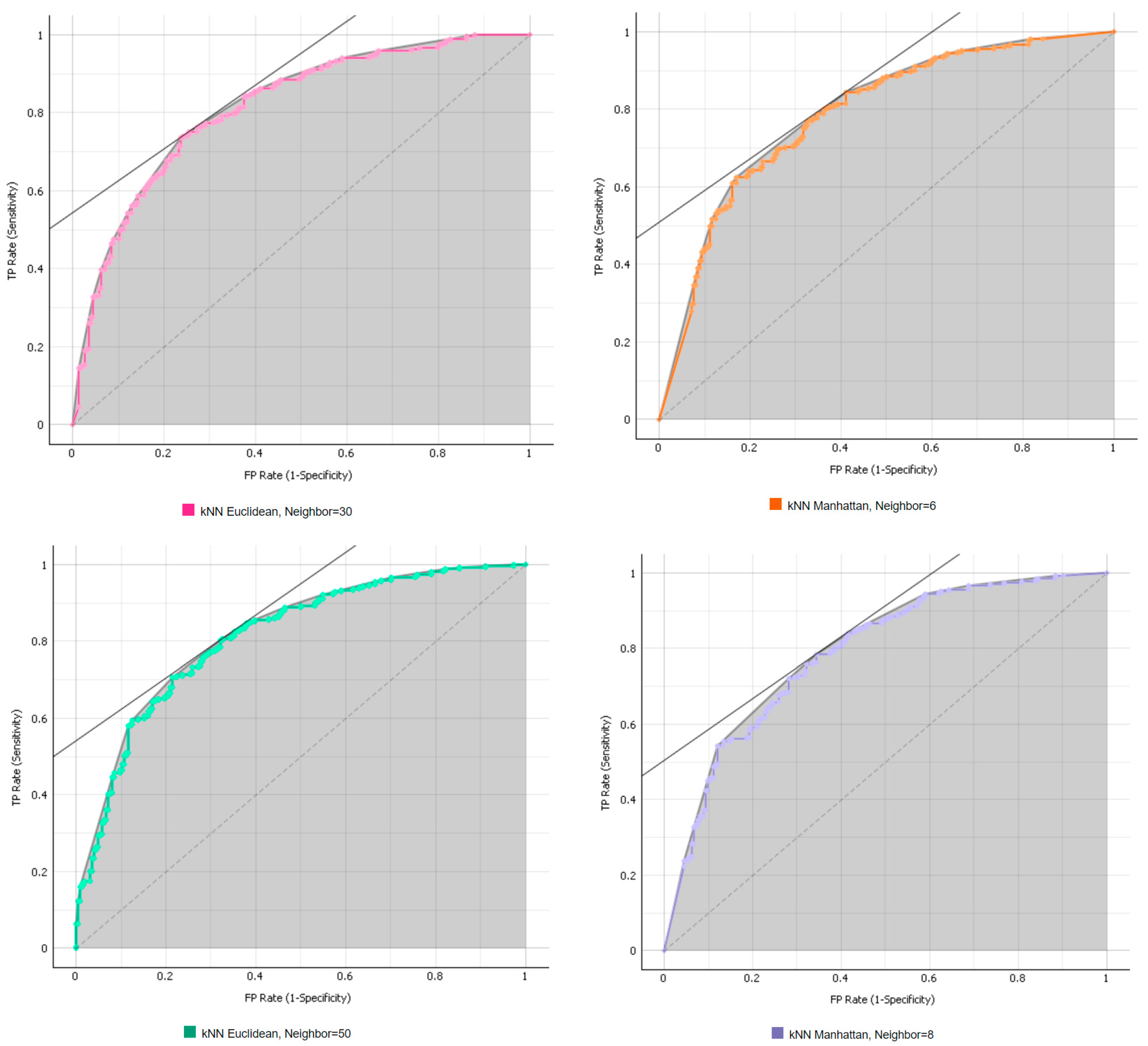
2.3.1. k-Nearest Neighbor (kNN)

As the name implies, kNN utilizes instance-based learning as a classification tool [33,34]. Instance-based learning means that the algorithm utilizes the vector space (i.e., space between objects) model, which makes kNN different from other classification algorithms. Because it relies on the vector space model, kNN can be utilized with cross-sectional data [35]. Various approaches can be used when assessing vector space [36]. When the outcome variable is categorical, Hamming distance can be utilized as shown in Equation (1):
H a m m i n g   d i s t a n c e = i = 1 I I n t ( x i y i )
where i indicates each observation; I is a set of observations i; x i and y i are the predictor and the outcome value with ith observation. When the outcome variable is a continuous variable, Euclidean distance, using the root of squared differences among observed samples, can be applied [37], or the Manhattan distance, using the absolute value of differences, can also be utilized as shown in Equations (2) and (3).
E u c l i d e a n   d i s t a n c e = i = 1 I ( x i y i ) 2
M a n h a t t a n   d i s t a n c e = i = 1 I | x i y i |
The combination of predictors and the outcome can be shown as ( x i , y i ) where i means the ith observation from the data (i = 1, 2, 3, … I). By using ascending order of distance, the observations can be allocated on a matrix as d x 1 ,   y 1   d x i ,   y i , where d is the distance from Equations (1), (2), or (3). When the outcome variable is categorical, the most frequent occurrence indicates the highest probability of belonging to the category shown in Equation (4). By using the probability, the expected category of the outcome is the maximum value from Function (4), as indicated in Equation (5):
p k ^ = i = 1 I ( y i = k ) i ~
y ^ = a r g m a x p k ^
where a predictor is a categorical variable from 1 to K, k means the kth category; p k ^ is the probability to be founded; and i is observed as the optimal observation ( i th). In the case that the outcome variable is a continuous variable, a certain number of observations are selected (n = i) from d x 1 ,   y 1   d x I ,   y I . The selected observations are utilized to calculate the inverse distance weighted average, which produces the predicted value of an outcome from Equation (6):
y ^ = i = 1 I 1 d ( x i , x ) y i i
As a classification algorithm, kNN is widely used for forecasting underweighted regression conditions. When kNN is combined with fuzzy vectoring, Östermark [38] suggested that kNN can be a useful tool for detecting data outliers, specifically when forecasting using finance and economic datasets. Because of the usability of kNN when making forecasts, this classification method has been adopted in various financial studies [39]. For instance, Meng et al. [33] adopted kNN to predict internet financial risk. They found an optimal number of categories for internet financial institutions. Phongmekin and Jarumaneeroj [40] utilized various algorithms (i.e., logistic regression, decision trees, Linear Discriminant Analysis, and kNN) to forecast stock exchange returns in Thailand. They found that kNN offers the best performance when predicting stock returns.

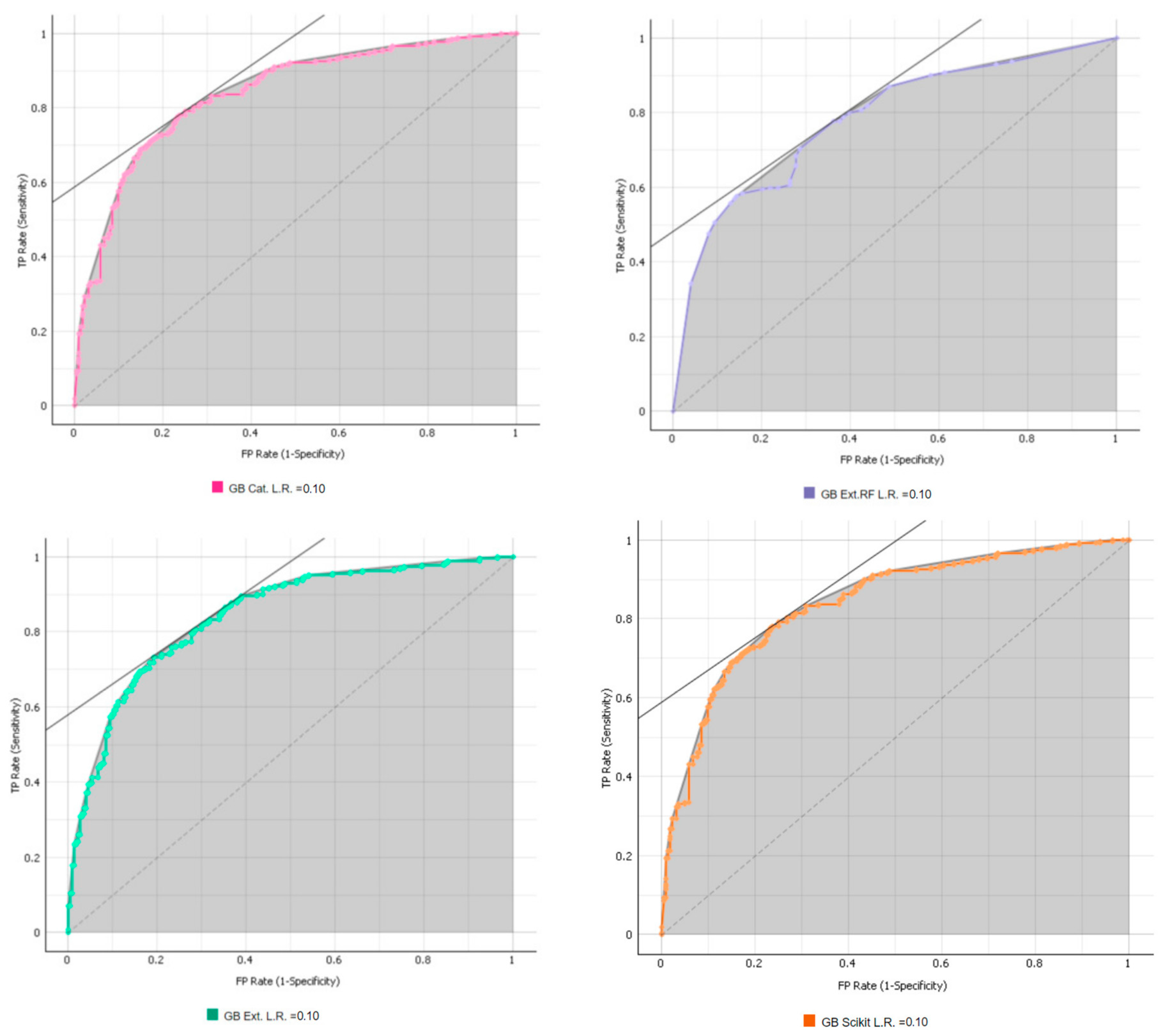
2.3.2. Gradient Boosting
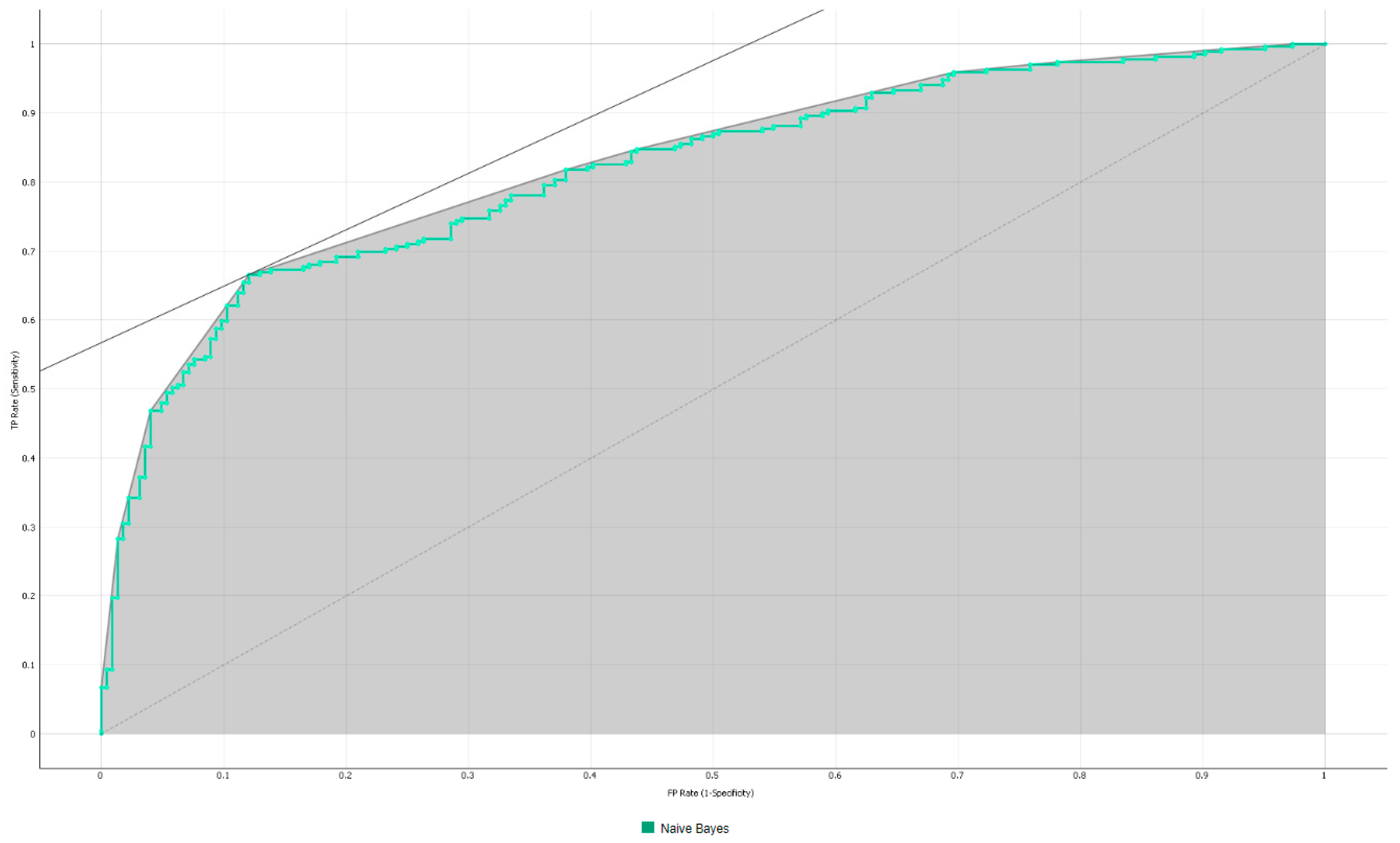
Gradient Boosting was introduced by Breiman [41], which was then merged with a regression algorithm developed by Friedman [42]. Gradient boosting is an ensemble modeling technique that combines classification and regression methods [42,43]. As the term ‘boosting’ implies, weak patterns from a dataset can be strengthened through a learning process when the goal is to find the highest probability of prediction [38]. ‘Gradient’ means an error from each strengthened stage gradually decreases until the lowest error level is reached [44]. The basic learning process begins by measuring the error (i.e., residuals) between a predicted value and an observed value [45], as shown in Equation (7), which is called a loss function:
l y i , f x i = 1 2 ( y i f ( x i ) ) 2
where i is the ith observation. The negative gradient format of Equation (7) produces residuals like those in Equation (8), which is a derivative of l y i ,   f x i :
δ y i , f x i δ f x i = y i f x i
As shown in Equation (8), the negative gradient produces a function similar to that of a regression residual (i.e., the difference between the predicted outcome and the actual outcome), which is how the name Gradient Boosting originated. Until the residuals are minimized, Gradient Boosting is iterated to make weak learners be combined, as shown in Equation (9):
y ^ = f x = k = 1 K L k + e
where k indicates each predictor; K is the optimal number to minimize the residual; and L k is each different weak learner. Usually, the weak learner is a tree model developed using a predictor.
In practice, there are multiple types of Gradient Boosting, including categorical Gradient Boosting, scikit-learn Gradient Boosting, Extreme Gradient Boosting, and Extreme Gradient Boosting with random forest. Categorical Gradient Boosting utilizes features as categories [46]. Scikit-learn gradient boosting is a type of Gradient Boosting algorithm offered in Python (https://scikit-learn.org/stable/ accessed on 1 November 2023), whereas Extreme Gradient Boosting is the most recent version of Gradient Boosting [9,47]. Each method was evaluated in this study.
The use of Gradient Boosting fits well with the research of interest in this study. Gradient Boosting is an ensemble model, which makes it particularly useful when conducting finance and business analyses [10,15]. Consider the work of Zhang and Haghni [15]. They utilized Gradient Boosting to improve travel time prediction in the transportation business. Specifically, they compared autoregressive integrated moving averages, random forest, and Gradient Boosting and concluded that Gradient Boosting showed better performance prediction. Guelman [10] investigated loss costs from Canadian insurers by comparing Gradient Boosting and a generalized linear model. Gradient Boosting was found to offer better performance in terms of prediction. Gradient Boosting has also been utilized in credit analyses. For instance, Chang et al. [44] compared various ML algorithms (i.e., group method of data handling, logistic, SVM, and Extreme Gradient Boosting). They observed Extreme Gradient Boosting to have outstanding performance when predicting credit risk. The approach has also been used to predict financial distress. Liu et al. [45] compared logistic, random forest, NN, SVM, and Gradient Boosting and noted that Gradient Boosting outperformed financial distress predictions. Carmona et al. [9] found the most impactful factors associated with bank failures using Gradient Boosting. Specifically, they compared bank failure prediction performance across logistic, random forest, and Extreme Gradient Boosting. They noted that Gradient Boosting provided the most meaningful insight when understanding bank failures.

2.3.3. Naïve Bayes

As the name implies, Naïve Bayes relies on Bayes’ theorem; sometimes researchers refer to the approach as Bayes or independent Bayes [48]. In practical applications, Naïve Bayes is useful for clustering and classification purposes [49]. All variables or features in a prediction model are assumed to be independent [50]. Naïve Bayes utilizes conditional probability modeling by combining various predictors ( X k   x 1 ,   x 2 ,   ,   x k ) with a set of probabilities ( p ( C m | X k ) ), where k is the number of predictors and m means the number of probabilities found. Because Naïve Bayes assumes the independence of all predictors, the maximized probability of having a certain value (or category) can be found using Equations (10) and (11):
p C m X i = 1 Z p ( C m ) k = 1 K p ( x k | C m )
y ^ = a r g m a x m 1 , , M p ( C m ) k = 1 K p ( x k | C m )
Some researchers have criticized the approach because the independent assumption is unnatural and unrealistic [51]. This is the reason that the approach is termed naïve. However, because of the assumption of independence, Naïve Bayes offers a mathematical transformation advantage, making the dataset analysis more predictable [51].
Naïve Bayes has been utilized in various financial studies as a classification algorithm. Jadhav et al. [12] compared the efficacy of SVM, kNN, and Naïve Bayes as algorithms to predict credit ratings. After comparing the algorithms, they concluded that Naïve Bayes performed best. Deng [52] utilized Naïve Bayes to detect fraudulent financial statements in auditing. Deng noted that Naïve Bayes can provide unique insights. Similarly, Viaene et al. [14] utilized Naïve Bayes to detect financial fraud (i.e., consumers’ faulty insurance claims). They concluded that the approach can improve prediction rates. Naïve Bayes has also been utilized in text classifications, such as when conducting a financial news analysis. Shihavuddin et al. [53] collected news articles about the Financial Times Stock Exchange 100 (FTSE100). Using Naïve Bayes, they concluded that not only does Naïve Bayes improve classification, but the approach can also be used to predict stock prices.

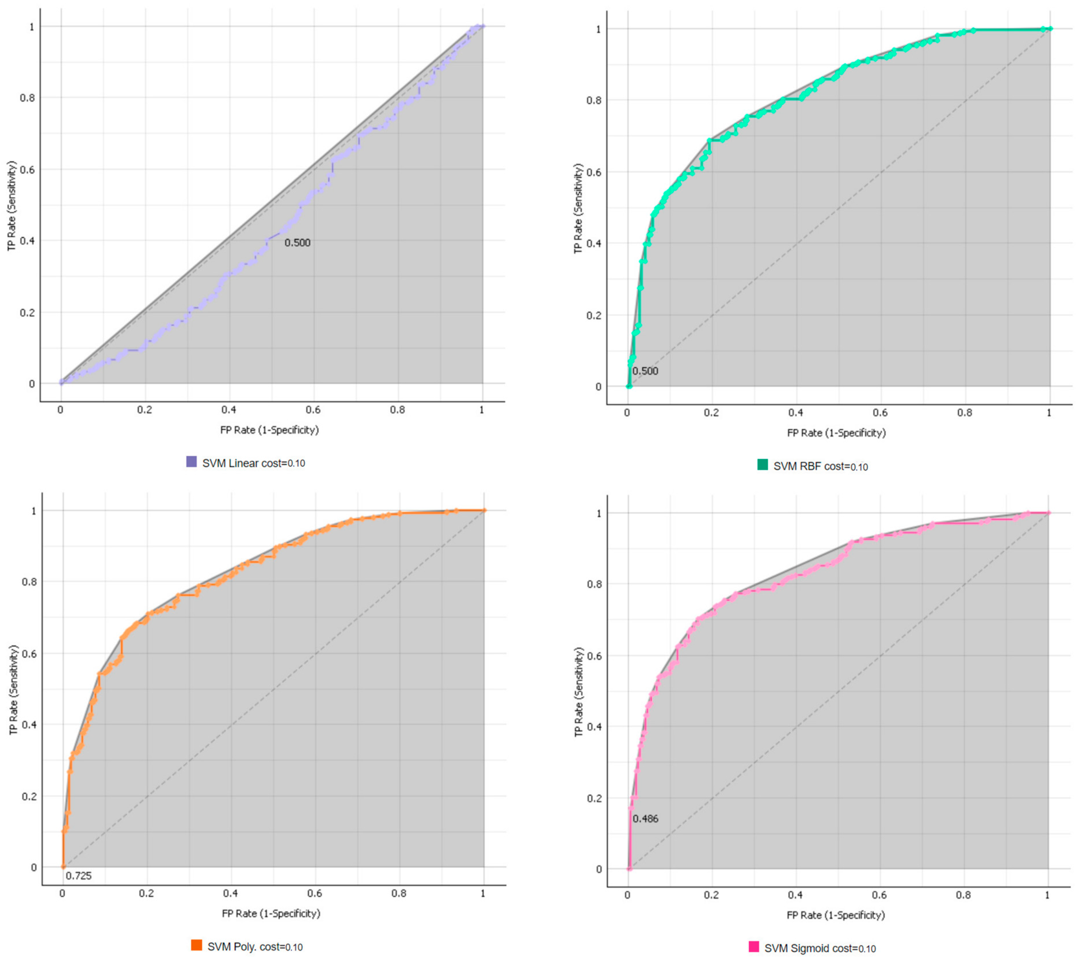
2.3.4. Support Vector Machine (SVM)

SVM classification is based on the concept of a hyperplane, which combines two separate classes [30]. The easiest way to understand classification by SVM is that a hyperplane is drawn among total samples. By drawing the hyperplane, two separate groups can be identified (e.g., upper and lower hyperplanes) as shown in Equations (12) and (13):
y = 1 ,   w h e n   [ B x k + a ] > 0
y = 1 ,   w h e n   [ B x k + a ] < 0
where k means each predictor and a is the constant in each hyperplane. Because of the complexities built into most datasets, the hyperplane is generally not well specified. Therefore, SVM sets the hyperplane by considering the maximum margin, the nearest vector from the potential hyperplane [54]. To draw a hyperplane when the maximum margin is found (Max M), SVM secures the optimal prediction performance. The function is shown in Equation (14), where B and a are assumed to be 1.00:
M a x   M ,   w h e r e   y k B x k + a M
In addition to a hyperplane and maximum margin in SVM, kernel functioning is often used to help classify samples when the dataset and vectors are highly dimensional [54]. Because one straight hyperplane cannot easily be optimally identified when the dataset is highly dimensional, different types of hyperplanes can be utilized, including linear (i.e., straight), polynomial, radial basis function (RBF), and sigmoid. These types function in the hyperplane, called a kernel [30]. In the current study, four types of kernels were utilized.
SVM has been utilized widely in credit risk studies [55]. For example, the approach has been employed to predict credit scores [56,57]. Baesens et al. [58] compared various algorithms (i.e., SVM, logistic, discriminant analysis, kNN, Neural Networks (NN), and decision trees) to predict credit scores. They found that SVM and NN showed the best prediction performance compared to the other algorithms. Yang [59] introduced an adaptive credit-scoring system using a kernel-based SVM. Yang noted that the non-linear feature of datasets can be managed through kernel transformation. Kim and Ahn [60] utilized various ML algorithms (i.e., multiple discriminant analysis, multinomial logistic analysis, case-based reasoning, and an artificial neural network) to examine corporate credit rates. They found that SVM outperformed in detecting multiclass classification of corporate credit ratings. Similar findings have been reported by Chaudhuri and De [61], Chen and Hsiao [62], and Hsieh et al. [63] when making bankruptcy and financial distress predictions.

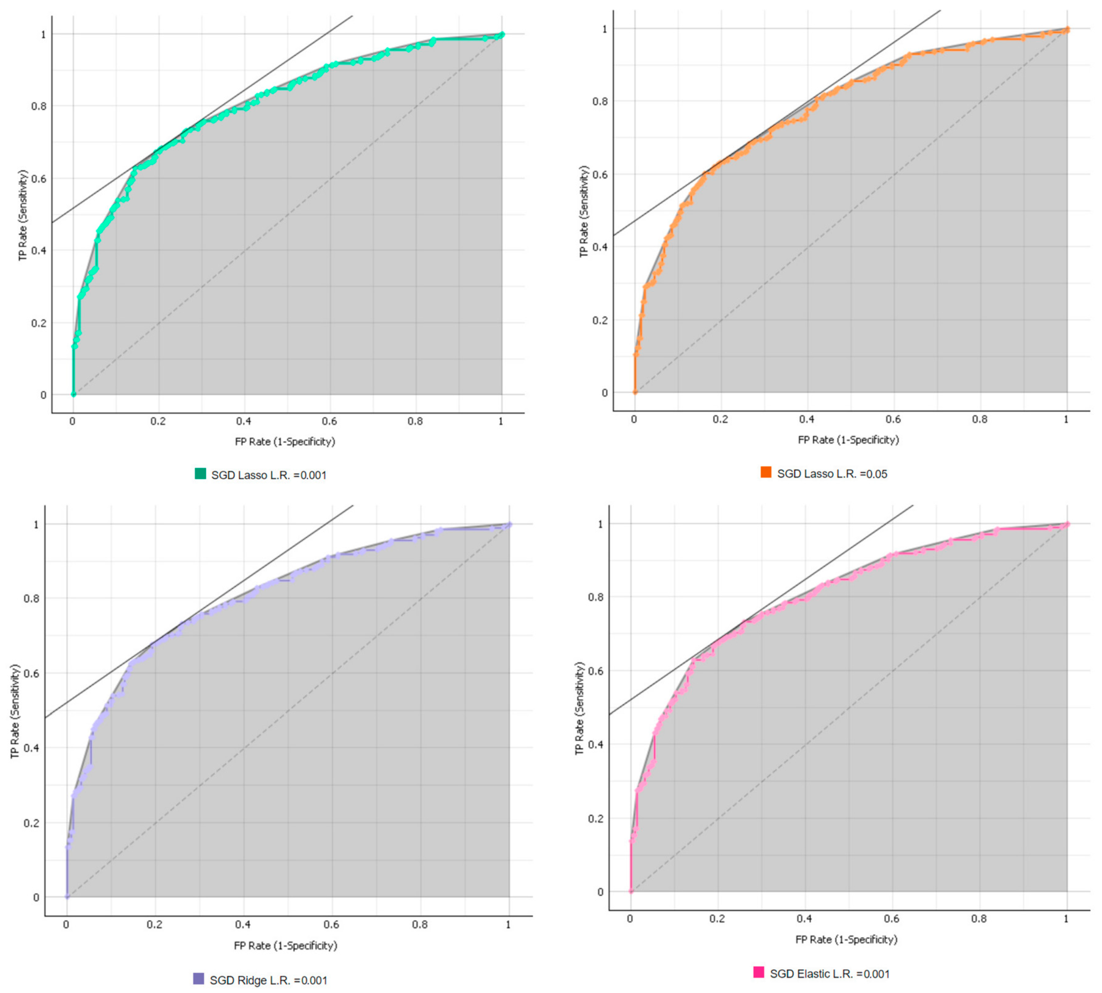
2.3.5. Stochastic Gradient Descent (SGD)

SGD emerged as an extension of previous theories, including the theory of adaptive pattern classifiers [64,65]. SGD is primarily used to help with data classifications. SGD begins by minimizing the errors (i.e., residuals) between predicted and observed values [66]. Specifically, SGD employs multiple iterations to minimize the errors in each gradient step [67] using Equation (15):
ϴ = ϴ η ϴ J ( ϴ )
where ϴ is the parameters of all networks from predictors; J ( ϴ ) is the loss function by using ϴ ; and η is the size of the learning rate. By repeating Equation (15), the parameters to minimize the value of the loss function can be estimated. SGD is popular because it is mathematically tractable and scalable [67]. Researchers like SGD because it helps solve optimization issues through stochastic approximation [68]. Because SGD relies on minimizing errors, regularization needs to be considered. Ridge and lasso are popular regularizations [69]. Elastic regularization can also be utilized [70]. The SGD approach can be employed when pre-selection or the transformation of explanatory variables is required and in situations where predictive machine learning scenarios are needed. The technique showcases robustness against outliers, as the steepest gradient algorithm emphasizes the correct classification of data points closely aligned with their true labels. As such, SGD extends beyond a mere method for optimizing objective functions with appropriate smoothness properties. SGD applies to a diverse set of machine learning prediction methods (e.g., [71,72]).
Similar to the other ML algorithms, SGD has been used in various consumer and finance studies. Deepa et al. [69] utilized SGD to predict the early onset of diabetes. Compared to logistic models, SGD showed a better prediction outcome. Using SGD algorithms, they noted that SGD can be used to enhance prediction rates.

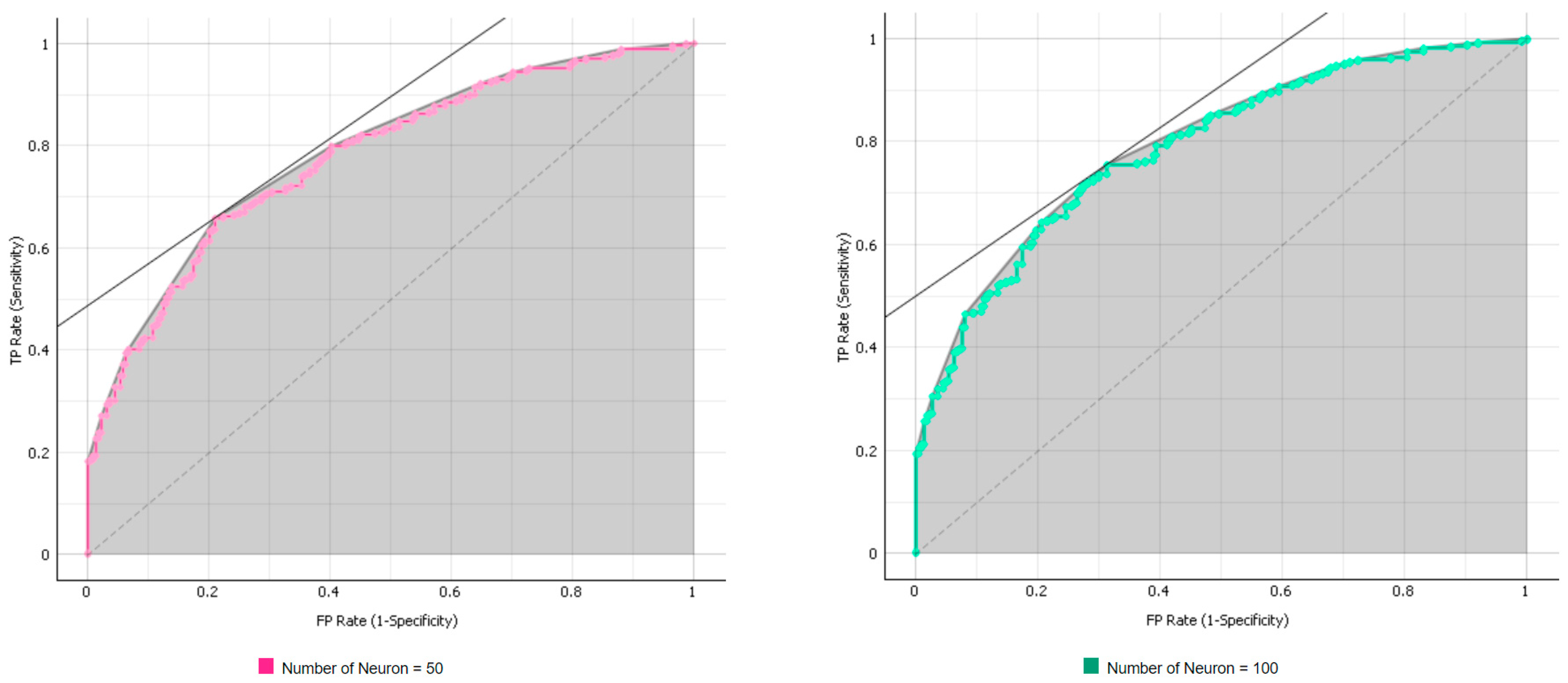
2.3.6. Neural Networks (NN)

NN is unquestionably the most mature of all algorithms within the ML area. NN offers flexibility when attempting to make classifications and when the goal of a project is to engage in future pattern recognition [25,26]. The uniqueness of NN is the approach’s use of neurons as hidden layers. Neurons resemble the human brain architecture [73]. Because of the unique architecture, all inputs (i.e., features or variables) are assumed to be connected to all neurons. All neurons are also assumed to be connected to all expected outcomes [6]. The basic function of NN is shown in Equation (16):
y = a ( k = 1 K w k x k + e )
where k denotes the predictors; w k is each predictor’s weight; and a is e bias like the error terms. Because of the complex connectivity through neurons between inputs and outcomes, NN can be expected to improve the prediction rate of outcomes. For instance, if five variables are used as inputs to predict two outcomes, employing four neurons, then there are 20 connections between the five variables and four neurons and an additional eight connections between the four neurons and two outcomes. This interconnectedness means 160 possible pathways from the five variables to the two outcomes through the four neurons. As this example illustrates, neurons make all connectivity from inputs to outcomes so that the prediction of outcomes can be improved.
The first step when conducting an NN analysis is to define the optimal number of neurons. Because NN can employ any possible number of neurons, the number of neurons should be tested first to find the best performing model [74]. In this study, the number of neurons was first tested, and then the optimal number of neurons was employed in the final model.
As noted above, NN is a very popular ML technique. NN has been utilized to predict credit scores and other consumer behaviors. Baesens et al. [58] compared various algorithms, including SVM, logistic, discriminant analysis, kNN, NN, and decision trees, to conclude that SVM and NN show the best prediction performance compared to the other algorithms. Some researchers have utilized NN to detect financial fraud (e.g., fraud reporting, fraudulent use of credit cards, fraudulent financial statements, fraud claims) (e.g., [74,75,76]), whereas others have utilized NN for the prediction of bankruptcy and financial distress [57,77,78]. Heo et al. [11] applied NN to predict the savings-to-income and debt-to-asset ratios among U.S. households. They compared the prediction accuracy between NN and conventional regression models and found that NN provides a deeper and more meaningful insight into the savings-to-income ratio and the debt-to-asset ratio.

2.3.7. Comparison Analysis

As alluded to in the preceding discussion, it is common for researchers to check whether ML algorithms enhance predictions by comparing outcomes to the results generated from a conventional analytic tool. When the outcome variable is binary, a logistic regression model [79] is most often the comparison. A logistic regression model can be estimated from Equation (17):
ln p x 1 p x = a + k = 1 K x k
where k denotes the predictors. This approach was taken in this study. Specifically, the ML algorithms’ predictions were compared to those predictions made using a maximum likelihood logistic regression.

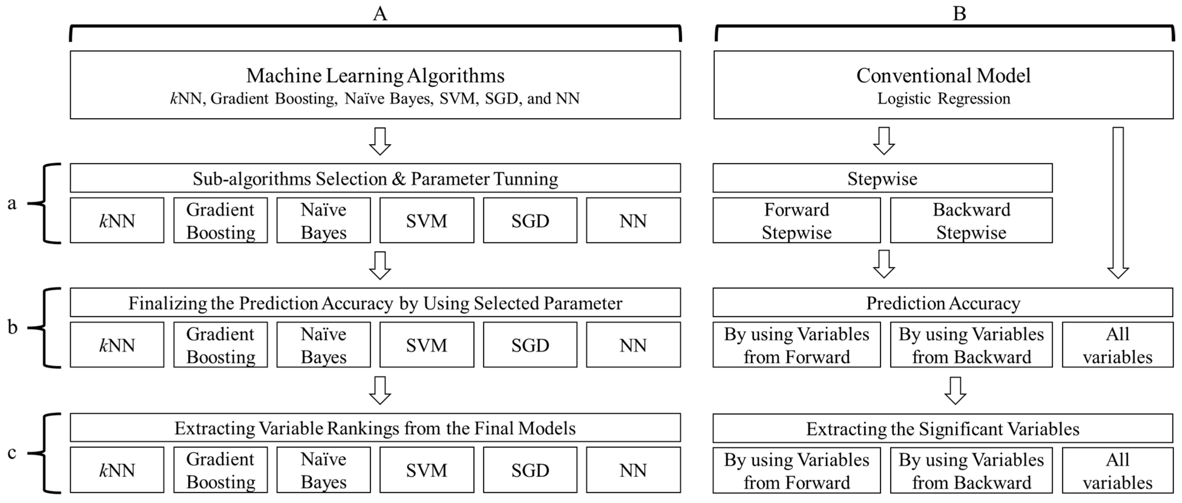
3. Empirical Model Flow

3.1. Research Purpose and Analysis Structure

The overarching purpose of this study was to determine which modeling technique offers the best prediction rate when describing the presence of an emergency fund. As noted above, this study employed and compared various ML algorithms. A four-step analytical process was used, and the steps are described below.
Step 1: Find the best parameters across the various ML algorithms
Multiple sub-algorithms exist within nearly all ML algorithms (Naïve Baynes is an exception). For instance, in terms of kNN, the Euclidean method and the Manhattan method can be used to measure distance. For Gradient Boosting, four sub-algorithms are widely used: categorical, Extreme, Extreme with random forest, and scikit-learn. In the case of SVM, the kernel can be assumed to be linear, polynomial, RBF, or sigmoid. Three sub-algorithms exist for SGD (i.e., elastic, lasso, and ridge). At this step of the analytical process, each sub-algorithm was tested. For the conventional analysis (i.e., logistic regression), three types of feature selection were utilized (i.e., all variables, forward stepwise selection, and backward stepwise selection).
In addition to sub-algorithms, each ML algorithm can be affected by internal settings (i.e., parameter settings). Based on the parameter setting, the same algorithm may exhibit different degrees of performance robustness [80]. To account for this possibility, this study tested different parameters for each algorithm. For kNN, normally, the number of neighbors can affect classification performance. Therefore, different numbers of neighbors (i.e., from 1 to 100) were employed and compared to find the best tuning for the kNN algorithm. Regarding Gradient Boosting, the learning rate may affect the algorithm’s performance. As such, various learning rate settings (i.e., 0.10, 0.15, 0.20, 0.25, and 0.30) were employed and compared to find the best application. For SVM, cost values are known to affect classification performance. To account for this, different cost values (i.e., 0.10, 1.00, 5.00, 10.00, 50.00, and 100.00) were employed and compared. It is also known that in terms of SGD, the learning rate may affect the algorithm’s performance. To deal with this possibility, various learning rate settings (i.e., 0.001, 0.005, 0.010, 0.050, and 1.000) were employed and compared. For NN, the number of neurons can change the algorithm’s performance. Therefore, different settings of neurons (i.e., 1, 5, 10, 15, 20, 25, 30, 35, 40, 45, 50, 55, 60, 65, 70, 75, 80, 85, 90, 95, and 100) were utilized and compared to find the best performance outcome. As shown in Figure 1 (Part A and Part B and Line a), the first step in the analysis involved selecting the best performing sub-algorithms and the best tuning for each algorithm.
Step 2: Find the best ML prediction algorithm among the various ML algorithms
It is important to note that assuming that one specific ML algorithm will ever show a dominant performance across predictions and classifications is unrealistic. Rather, by the topical issue type and the predictive dataset’s nature, diverse ML algorithms can be expected to show better/worse prediction and classification performance [27]. Given the binary feature of the dependent variable in this study, various classification algorithms were selected, as explained above. As shown in part A with line b in Figure 1, the second step in the analytical process involved finding the optimal ML algorithm from the selected six ML algorithms. The best prediction performance was selected as the most appropriate for use within the dataset.
Step 3: Check whether ML accuracies are higher than those offered by a conventional analysis
Even if a selected ML algorithm shows excellent performance across tested ML algorithms, the prediction function may actually offer a lower level of prediction when compared to a conventional analytical technique like logistic regression. Therefore, the third step involves comparing the prediction performance of the selected ML algorithm and the conventional analysis (see parts A and B with line b, Figure 1).
Step 4: Determine which factors are associated with holding an emergency fund
Assuming the selected ML algorithm performs better than the conventional analysis, the influencing rank of input factors can be found by evaluating algorithm outcomes. The influencing rank can be viewed similarly to the significant variable list from a regression model, or the rank can differ. By checking the similarity or differences between the rank of influencing factors (ML algorithm) and the significant factors (logistic regression), it is possible to establish variable importance and possible linkages across variables that can then be examined at a later date. This step in the analytical process is crucial because some variables that emerge from an ML algorithm may not be significant in a traditional sense. Therefore, as shown in Figure 1 (line c for both parts A and B), the final step involves checking the variable list generated from the ML algorithms and the logistic analysis.

3.2. Analytic ML and the Conventional Analysis Process

Each ML algorithm test was conducted by dividing the sample into a training dataset and a test dataset. As shown in Figure 2, using the training dataset, each ML algorithm was used to identify the best prediction model. Data were split into training and testing datasets using a 50:50 random split ratio. As noted by Joseph [81], the split ratio varies by study and typically ranges from 80:20 division, 70:30, 60:40, and 50:50. The literature shows a conspicuous absence of definitive guidelines delineating the optimal or preferred data split ratio for a given dataset. As such, based on the comparatively small size of the dataset used in this study, the research team concluded that a 50:50 ratio was appropriate (see also [82,83]). Moreover, this ratio split allowed for robust validation of the data (i.e., k-fold validation). After a model was identified, the test dataset was utilized to validate the results from the test. If the model still showed a robust prediction outcome, the model was defined as optimal. The Python with Orange 3 visualization tool was used for all the tests. The conventional analysis utilized a similar procedure. A logistic regression model was estimated utilizing the training dataset. Results were validated using the test dataset. Stata 17.0 was used to estimate the models.

3.3. The Accuracy Estimation Method

To measure prediction accuracy, a receiver operator characteristics curve (ROC curve) and the area under the ROC curve (AUC) methodological approaches were utilized. An ROC curve is produced using two inputs: a true positive (TP) rate and a false positive (FP) rate [84]. The TP rate is calculated as the ratio between positive (i.e., correct) classifications and total positives. The FP rate is calculated using the ratio between negative (i.e., incorrect) classifications and total negatives. This indicates a more precise estimate when the TP rate is close to 1.00. The approach is also more precise when the FP rate is close to zero. An ROC curve shows the TP rate on the vertical axis and the FP rate on the horizontal axis. When an ROC curve shows a convex shape upward to the left, the accuracy is considered to be more precise. Additionally, the area under the curve is called the AUC, which indicates the power of the ROC (i.e., measured as 0.00 to 1.00) [44]. If the ROC curve has a vertical axis with a TP rate (i.e., zero to 1.00) and a horizontal axis with a FP rate (i.e., zero to 1.00), the area can be calculated from zero (zero times zero) to 1.00 (one times one).

3.4. The Factor Ranking Method

In Step 4, the rank of variables, in terms of prediction, is represented numerically (i.e., RReliefF). Whereas predictors in a logistic analysis can be evaluated using significance/insignificance estimates and marginal effects (i.e., coefficients), identifying high-ranking predictors using ML algorithms is more complex. For example, in the case of NN, all input variables connect to the outcome variable through neurons. Multiple weights are connected between a particular input variable and the outcome variable. There is not a specific number. As such, the evaluation of ML algorithms tends to focus on the complex combinations of input factors and the effects of variables on an outcome variable instead of the unique association between an input variable and the outcome variable.
For this study, variable ranks were identified using RReliefF. RReliefF is an advanced version of Relief [85] and ReliefF [86], which are generally accepted attribute estimators. Relief is the baseline of RReliefF. Robnik-Šikonja and Kononenko [87] introduced RReliefF, which was developed from Relief. The diff function, as shown below, can be used to better understand the baseline of RReliefF. The diff function is used to measure the distance among instances, which can be used to identify the nearest neighbors [87]. Equation (18) is used for categorical attributes, and Equation (19) is for continuous attributes:
d i f f A ,   I 1 ,   I 2 = 0 ; v a l u e   A ,   I 1 = v a l u e   ( A , I 2 )   1 ;   o t h e r w i s e
d i f f A ,   I 1 ,   I 2 = | v a l u e   A ,   I 1 v a l u e   A , I 2 | max A m i n ( A )
These equations are used when investigating a dataset that comprises multiple examples, denoted as I1, I2, ..., In, situated within an instance space. Each example is characterized by a set of attributes, represented as Ai, where attributes are associated with each example. By using the diff function, the weight (W) of attribute A can be estimated as Relief by following Equation (20) [86]:
W A = P d i f f .   v a l u e   o f   A     n e a r e s t     i n s t a n c e   f r o m   d i f f .   c l a s s ) P d i f f .   v a l u e   o f   A     n e a r e s t     i n s t a n c e   f r o m   s a m e   c l a s s )
Based on the fundamental Relief framework, regressional ReliefF was introduced using Equation (21):
W A = P d i f f . r e s p o n s e     d i f f .   v a l u e   o f   A   a n d   n e a r e s t   i n t a n c e s ) P d i f f .   v a l u e   o f   A     n e a r e s t   i n s t a n c e s ) P d i f f .   r e s p o n s e     n e a r e s t   i n s t a n c e s ) ( 1 P d i f f . r e s p o n s e     d i f f .   v a l u e   o f   A   a n d   n e a r e s t   i n t a n c e s ) ) P d i f f .   v a l u e   o f   A     n e a r e s t   i n s t a n c e s ) 1 P d i f f .   r e s p o n s e     n e a r e s t   i n s t a n c e s )
Compared to other attribute estimators (e.g., the root mean of squared error and mean absolute error), the RReliefF estimator uses a factor measured by considering interactions with other factors. RReliefF measures a factor’s estimator contextually. A higher RReliefF number for a specific variable indicates that the factor is expected to predict the outcome with better (optimized) performance. Therefore, in this study, RReliefF was used to check the factors’ ranking.

4. Data and Measurement

4.1. Data

Data were collected in 2021 using an online survey distributed in the United States. A survey agency invited 5900 consumer households to participate in this study; 1000 respondents answered all the questions; however, 13 respondents provided inaccurate information (e.g., reporting two years old for their age), which resulted in a useable sample of 987. Descriptive information for the sample is shown in Appendix A Table A1.

4.2. Measurement

The outcome variable was whether a respondent held an emergency fund or not. The variable was coded dichotomously (Have = 1; Not have = 0) based on an answer to the following question, “Have you set aside emergency or rainy day funds that would cover your expenses for three months, in case of sickness, job loss, economic downturn, or other emergencies?”.
The input variables (i.e., predictors) were split into the following five categories in alignment with [88] and [89]: (a) financial statements and resources, (b) financial literacy and education, (c) psychological factors, (d) demographic factors, and (e) COVID-associated factors (used to account for the period of data collection).
The following binary-coded variables comprised the financial statements and resources category: (a) have auto loan or not; (b) have student loan or not; (c) have farm loan or not; (d) have equity loan or not; (e) have mortgage loan or not; (f) own house or not; (g) have saving account or not; (h) have checking account or not; (i) own term life insurance or not; (j) own whole life insurance or not; (k) ever use payday loan; and (l) have health insurance or not. In addition, a categorical variable was included to account for the possibility of receiving financial advice for making financial decisions (i.e., 1 = have; 2 = do not know; 3 = no). Finally, a respondent’s physical distance from their closest financial professional was asked and coded as follows: 1 = less than 5 miles; 2 = 5 to 10 miles; 3 = 10 to 20 miles; 4 = 20 to 50 miles; 5 = over 50 miles; and 6 = n/a or do not know.
Three variables comprised the financial literacy and education category: (a) had financial courses in high school (1 = Yes; 0 = otherwise); (b) had financial courses in college (1 = Yes; 0 = otherwise); and (c) objective financial literacy. The objective financial literacy variable was based on answers to three true/false questions [90], resulting in scores that could range from 0 (no correct answers) to 3 (all correct answers).
The psychological factors category was comprised of the following variables: (a) financial risk tolerance; (b) financial satisfaction; (c) financial stress; (d) financial self-efficacy; (e) locus of control; (f) life satisfaction; (g) the Rosenberg self-esteem scale; and (h) job insecurity. Financial risk tolerance was assessed using the Grable and Lytton’s risk-taking propensity scale [91]. Scores ranged from 13 to 42. Financial satisfaction was measured using seven items on a five-point scale (min = 7; max = 35) (see [92]). Financial stress was measured using 24 items on a five-point scale (min = 24; max = 120) (see [88]). Financial self-efficacy was measured using six items, also on a five-point scale (min = 6; max = 30) (see [93]). Locus of control was measured using seven items on a five-point scale (min = 7; max = 35) (see [94]). Higher scores were representative of an external locus of control. Life satisfaction was measured using seven items on a seven-point scale (min = 5; max = 35) (see [95]). Self-esteem was measured with Rosenberg’s 10-item scale that was assessed using a four-point scale (see [96]). Finally, job insecurity was measured using seven items on a five-point scale (min = 7; max = 35) (see [97]).
Demographic factors included (a) a variable representing the region of the country where a respondent lived, (b) work status, (c) agricultural working status, (d) education level, (e) marital status, (f) gender, (g) age, (h) whether a respondent lived in an urban area, (i) ethnicity, (j) income level, (k) number of children in a respondent’s household, and (l) perceived health status. The region represented a respondent’s state of residence. Work status was coded categorically as 1 = Full-Time; 2 = Part-Time; 3 = Self-Employed; 4 = Homemaker; 5 = Full-Time Student; and 6 = Not Working. Agriculture working status was coded as a categorical variable (1 = farm; 2 = ranch; 3 = agri-business; and 4 = not working in agriculture). Education level was coded categorically as 1 = high school or lower; 2 = some college; 3 = college; and 4 = postgraduate. Gender was coded as female or otherwise. Marital status was coded as a binary variable (i.e., single or otherwise). Age was measured in years. Living in an urban area was coded categorically as follows: 1 = urbanized area of 50,000 or more people; 2 = suburban area, near urbanized area with at least 2500 and less than 50,000 people; and 3 = rural area, all population, housing, and territory not included within any urban areas). Ethnicity was coded as a categorical variable, where 1 = White or Caucasian; 2 = Hispanic or Latino/a; 3 = Black or African American; 4 = Asian; 5 = Pacific Islander/Native American or Alaskan Native; and 6 = Other. Income level was coded categorically as 1 = Less than USD 15,000; 2 = USD 15,000 to USD 25,000; 3 = USD 25,000 to USD 35,000; 4 = USD 35,000 to USD 50,000; 5 = USD 50,000 to USD 75,000; 6 = USD 75,000 to USD 100,000; 7 = USD 100,000 to USD 150,000; and 8 = Over USD 150,000. The number of children living in a respondent’s household was measured as a reported number. Finally, the perceived health status of a respondent was measured as a categorical variable (i.e., 1 = Excellent; 2 = Good; 3 = Fair; and 4 = Poor).
Finally, COVID factors were measured with items that asked how a respondent was affected by the COVID-19 virus and pandemic, how long a respondent expected the COVID-19 pandemic to last, and the receipt and timing of a stimulus check. The following items were used to evaluate perceptions of the COVID-19 pandemic: (a) how a respondent’s financial situation was affected by COVID-19; (b) how a respondent’s health condition was affected by COVID-19; (c) how a respondent’s general well-being was affected by COVID-19; and (d) how a respondent’s work–life balance was affected by COVID-19. Answers were coded as 1 = almost no impact to 4 = serious impact. Perceptions about the duration of the pandemic were assessed by asking if (a) my financial situation will get better, get worse, or stay the same in three months; (b) my financial situation will get better, get worse, or stay the same in six months; or (c) my financial situation will get better, get worse, or stay same in one year. Answers were coded as 1 = get better; 2 = get worse; or 3 = stay the same. The timing of receiving a stimulus check was measured nominally as 1 = get stimulus check in April; 2 = get stimulus check in May; 3 = get stimulus check in June; 4 = get stimulus check in July; 5 = get stimulus check after July; 6 = do not know; 7 = do not want to answer; 8 = had not received stimulus check yet; and 9 = not eligible for a stimulus check.

5. Results

5.1. Identify the Best Parameters among the Various ML Algorithms

The first step in the ML analyses began by finding the best parameters and tuning the algorithms. Across the six ML algorithms, various parameters were tested and tuned. The tuning procedure is shown in Appendix B.

5.2. Results for Step 2: Find the Best ML Prediction Method among the Various ML Algorithms

It was determined that kNN and NN overfit the data somewhat. For example, the prediction accuracy (AUC) of both algorithms were strong when the models were built; however, the prediction accuracy was weakened when tested. Gradient Boosting offered the best performance with categorical consideration and a learning rate of 0.10 (see Table 1). However, kNN and SVM were still robust. Figure 3 shows the selected algorithms’ ROC curves from the six ML algorithms.

5.3. Results for Step 3: Check Whether the Accuracy of the ML Algorithms Is Higher Than the Accuracy Offered by a Logistic Regression

Table 2 shows the results from the logistic regression. As shown in Table 2, none of the variables had a significant effect in describing whether a respondent held an emergency fund. However, when the variables were added using a stepwise variable selection approach, several variables (i.e., savings account, mortgage loan, whole life insurance, no access to financial advisor, financial course in high school, financial satisfaction, financial self-efficacy, life satisfaction, number of children, and financial situation during the COVID-19 pandemic) were observed to be statistically significant.
Based on a sample size of 477, ROC graphs and AUCs (i.e., predictions made from the test dataset) are shown in Figure 4. The predictions resembled convex curves. The upper left ROC was made when all variables were included in the prediction; the lower left ROC was estimated when backward stepwise was utilized; the right upper ROC was made when forward stepwise was utilized.
As shown in Table 3, AUC was under 0.800, which was lower than the ML AUC predictions. Even the worst performing ML exhibited a better AUC (i.e., 0.793 when ML was NN) compared to results from the logistic regression models (i.e., 0.754 when the variable list was determined via backward stepwise variable selection). This means that conventional analysis is proper when the research goal involves identifying significant variables; however, when the research goal involves maximizing prediction performance, ML algorithms provide a more robust insight into behavior (i.e., prediction accuracy can be maximized using ML techniques).
Table 3 indicates that machine learning (ML) offers more (i.e., efficient) predictive performance than a logistic regression methodology. However, this does not necessarily mean that ML provides a better explanation. As previously explained, ML has the advantage of making better predictions by including more variables, as it incorporates the covariances inherent in each variable into a prediction. This means that some important features with higher prediction weights are selected based on the covariance with other features. On the other hand, generalized linear models like logistic regression exclude covariances other than the unique covariance between an outcome and input variables. Traditional regression techniques focus on finding precise explanations for individual variables. This ultimately leads to an increase in explanatory power but a decrease in predictive power. Therefore, the results shown in Table 3 signify an improvement in the predictive power of ML but do not necessarily mean that the explanatory power of individual variables has improved.
For example, when looking at Table 2 (i.e., results from the logistic regression), variables that have a significant relationship with holding an emergency fund are easily identified. Most of these variables, including a household’s financial situation, number of children, and holding a savings account, match with what has been reported in the previous literature. The explanatory power of these variables remains valid. However, Table 4 shows how different variables influenced these predictive performances. When comparing Table 2 and Table 4, it becomes apparent that variables that were significant in Table 2 do not always have high predictive weights in Table 4. This indicates that in the case of the important variables shown in Table 4, various variables, as assumed by complex system science models and ecological system theory, contribute to better predictions. Therefore, the high predictive power in Table 3 and the variable rankings in Table 4 can play a role in identifying variables that conventional analyses, such as logistic regression, may overlook conceptually or theoretically. While ML may provide high predictive power, variables that were not statistically significant in the logistic regression (e.g., region, education level, financial self-efficacy, having a financial advisor, and farm loan) should be reconsidered as potentially important variables based on their high predictive weights, despite being overlooked in previous studies.

5.4. Results for Step 4: Determine Which Factors Are Associated with Holding an Emergency Fund

Table 4 shows the ranking importance of the best fitting ML algorithm (i.e., Gradient Boosting) across the variables evaluated in this study (i.e., RReliefF). Education level and having completed a financial course while in college ranked highly. This implies that educational attainment is important in helping someone gauge the need for an emergency fund. In addition, this indicates that promoting financial education, both in formal academic settings and through specialized courses, can be an effective strategy when encouraging individuals to (a) recognize the importance of emergency funds and (b) take proactive steps to establish emergency savings. Policy makers and educators should consider expanding financial education programs to enhance financial preparedness.
In addition, some financial-related psychological factors (i.e., financial satisfaction, financial self-efficacy, and financial stress) were found to be important. This implies that these factors are associated with holding an emergency fund. Financial institutions, financial service providers, and financial educators should incorporate psychological aspects into their financial literacy and counseling programs. Fostering financial satisfaction and self-efficacy while addressing financial stress is likely to help individuals develop positive emergency fund attitudes and behaviors.
Interestingly, COVID-19-related factors were not particularly important predictors in the model. This suggests that households are unlikely to change their emergency fund saving behavior even in the context of situational influences like a challenging economic situation.
Although Gradient Boosting was deemed to be the best model, the other ML algorithms produced comparable results. For instance, owning whole life insurance was an important variable when describing who holds an emergency fund across the model. This indicates that those who own whole life insurance are more concerned about their future self and the financial welfare of other household members (i.e., individuals who own life insurance generally exhibit a heightened awareness of their long-term financial security and the financial well-being of their family). Financial service providers can use this insight to emphasize the importance of comprehensive financial planning, including both insurance and emergency fund considerations. Similarly, educational factors (i.e., education level, completing a financial course in high school, or a financial course while in college) were found to be important predictors across the ML algorithms.
The ML results differed in significant ways from the logistic regression estimates. Compared to the Gradient Boosting model, taking a financial course in college and financial stress were unimportant in the logistic regression. Even so, there were some similarities. For instance, owning whole life insurance, taking a financial course in high school, and financial satisfaction ranked highly across the models. This indicates theoretical connections between these variables and holding an emergency fund. This study illustrates that combining insights from different analytical approaches can lead to a more comprehensive understanding and effective promotion of emergency fund savings.

6. Discussion

ML and big data analytical techniques have, over the past decade, garnered increasing attention among researchers, educators, and policy makers as a way to obtain deeper insight into social science phenomena. This study adds to the growing consumer studies methodological literature by illustrating how ML techniques can be applied to assessing household consumer attitudes and behaviors and how ML methods can improve prediction rates.
The outcome variable in this study was whether a household held an emergency fund, which was used to indicate a household’s degree of financial preparedness. The existing financial ratio literature is relatively consistent in reporting that those who hold emergency savings share a common demographic profile [3,4]. They tend to have high income, are more educated, and have greater wealth. It is important to note, however, that nearly all profiles reported in the literature were constructed using traditional methodologies, primarily regression techniques. At the outset of this paper, it was hypothesized that while existing profiles may remain valid, other variables might also be influential in describing who does and does not hold emergency savings. Traditional regression modeling techniques do not account for hidden layers between and among variables. While it is possible to create moderation and mediation models, to do so with large data is nearly impossible when the constraints associated with regression modeling are applied. This study’s methodological approach dealt with this issue by showing that when prediction or profiling is the main purpose of a study, ML algorithms can provide a more nuanced insight into consumer behavior compared to more commonly used statistical analysis techniques [7,16].
This study compared and tested several ML algorithms to determine which offers the most robust prediction rate. The ML algorithm outputs were compared to estimates derived from logistic regression models. Several takeaways emerged from these analyses. First, those using ML techniques must know that parameter tuning is not optional. Incorrect parameter tuning results in lowered prediction and classification rates. Those who adopt ML algorithms in consumer studies should consider this point and compare tuning performance when conceptualizing studies. Second, sub-algorithms should be considered. Using an incorrect sub-algorithm will almost always lower prediction and classification validity. Third, when evaluating ML algorithm outputs, it is important to remember that ML algorithms do not show marginal effects. Instead, ML algorithms provide a ranked ordering of predictors. As such, the interpretation of an ML analysis should not be considered deterministic. Instead, the interpretation of an ML output needs to be conceptualized as more in line with an explorative introduction.
In this study, Gradient Boosting, kNN, and SVM were found to provide the most robust degrees of prediction and classification. Gradient Boosting offered the best prediction rate, which aligns with what others have reported in the literature (e.g., [9,10,15,44]). Gradient boosting is an ensemble modeling technique that integrates classification and regression methods [42,43]. The ensemble of classification and regression estimation works well when optimizing prediction accuracy [31] and minimizing error levels [44]. What is particularly interesting in this study is that income and wealth—factors generally considered the most descriptive of financial preparedness—were not highly ranked in the Gradient Boosting algorithm, nor with kNN or SVM. This insight differs from what is generally shown using regression techniques [3]. However, educational factors and the existence of financial obligations were more important. It appears that a consumer must possess the financial literacy to anticipate the need for emergency savings, formulate a plan to build an emergency fund, and implement the plan. The consumer must also have an objective reason to hold emergency fund assets. The existence of loans is one reason a consumer may opt to hold assets in an emergency fund. Likewise, a consumer needs to hold an attitudinal disposition that values one’s future self or the well-being of household members. The consistently high ranking of life insurance in the ML algorithms suggests that the ability to plan for the future is an important characteristic among those holding emergency fund assets. The region variable in the kNN model is worthy of future research. The variable represents the state where a respondent resided at the time of the survey. It appears that some consumers are more likely than others to take financial preparedness steps. Specifically, those living in rural areas who also hold existing debt, are predicted to be more likely to hold an emergency fund.
This study represents a noteworthy advancement in consumer studies literature, particularly in the domains of personal finance and financial planning. This paper illustrates the value of ML techniques when predicting behavior. While numerous researchers have utilized ML methodologies with social science datasets (e.g., [9,10,11,12,13,14,15]), these efforts have sometimes suffered from limitations, such as their inability to comprehensively compare diverse ML methods or their focus on non-household factors. This means that the practical relevance of findings about household financial management has notable limitations. This paper is one of the few studies to comprehensively analyze the nuances associated with holding an emergency fund at the household level.
Another significant contribution of this paper is the expanded scope of variables that were used to predict holding an emergency fund. Rather than rely on a limited set of preexisting variables as described in the literature (i.e., primarily financial factors and sociodemographic attributes) (e.g., [3,4]), this study introduced a broader range of variables, including financial education, psychological aspects, COVID-19-related factors, distance to financial service providers, and holding various types of loans. This approach aligns well with ML’s capacity to leverage multiple variables [16], potentially unveiling overlooked variables that could significantly contribute to understanding the dynamics of emergency fund management.
Moreover, this study departs from the prevailing practice of assuming linear relationships between and among variables. The ML technique uses a pattern recognition and classification approach, making it possible to move beyond traditional linear assumptions. To achieve this, six distinct ML algorithms were employed as complex systems science models. The application of these algorithms allowed for a comprehensive investigation of the potential contributions of ML to the field of consumer studies. Notably, each ML algorithm underwent meticulous parameter tuning and calibration, extending beyond algorithmic utilization to demonstrate the application of ML techniques to address complex questions. The comprehensive approach in this study underscores the commitment to advancing the understanding of emergency fund management dynamics and enhancing the practical applicability of ML in consumer studies.
In summary, the results from this study advance the methodological body of literature for those working in the consumer studies field. This study shows that ML algorithms can be used to improve predictions and classifications of consumer attitudes and behaviors. Future research should align the results from this study with existing models and profiles of those who hold emergency savings. Information from such studies can be used by financial educators, consumer advocates, and policy makers when helping households achieve greater levels of financial preparedness.

7. Conclusions

This study is noteworthy in making significant theoretical, practical, and methodological contributions to consumer studies. The theoretical contribution lies in its application of ML techniques to the study of household financial decision making. Unlike traditional linear models, this study used a pattern recognition and classification methodology, shedding light on the intricate complexities underlying emergency fund management. The findings from this study challenge conventional beliefs by highlighting the importance of financial literacy, financial obligations, and a positive attitude towards future financial well-being as key factors in predicting who is more likely to hold emergency savings, with income and wealth taking a secondary role.
On a practical level, findings from this study underscore the critical importance of parameter tuning and sub-algorithm selection when employing ML techniques in consumer studies. This paper offers valuable insights into the use of ML algorithms when predicting and classifying consumer attitudes and behaviors, which can have direct applications for financial service providers, financial educators, consumer advocates, and policy makers. Moreover, this study expands the spectrum of variables considered, incorporating financial education, psychological factors, COVID-19-related variables, and others, thereby enhancing the predictive capacity of models to understand the dynamics of emergency fund management.
Even in the context of these significant contributions, limitations need to be acknowledged. ML techniques, while improving prediction rates, do not readily provide straightforward marginal effects. Thus, some researchers use ML algorithms as a starting point in identifying key variables for use in secondary models. While this study evaluated six robust ML algorithms, including Gradient Boosting, kNN, and SVM, further research is needed to determine when one particular approach should be used to address a specific research question. Further advanced ML algorithms, such as Generative Adversarial Network, Recurrent Neural Network, or Convolutional Neural Network, should be evaluated in future studies. In the context of this study, additional research is needed to decipher regional variations in holding an emergency fund. Future studies should also aim to integrate the findings with existing models and profiles of emergency savings holders. Doing so will contribute to a better understanding of the financial preparedness of households. In addition, the current ML algorithms are all well-known algorithms. Even in the context of these limitations and opportunities for future work, this study advances the consumer studies methodological landscape by showcasing how ML techniques can enrich the field’s comprehension of consumer attitudes and behaviors, particularly within the context of holding an emergency fund.

Author Contributions

Conceptualization, W.H. and E.K.; methodology, W.H. and E.K.; software, W.H. and E.K.; validation, W.H., E.K., E.J.K. and J.E.G.; formal analysis, W.H.; investigation, E.K.; data curation, E.J.K.; writing—original draft preparation, W.H., E.K., E.J.K. and J.E.G.; writing—review and editing, W.H., E.K., E.J.K. and J.E.G.; supervision, W.H. and J.E.G.; funding acquisition, W.H. All authors have read and agreed to the published version of the manuscript.

Funding

This work is supported by the USDA National Institute of Food and Agriculture, Hatch project 1017028 and Multistates project 1019968.

Data Availability Statement

The research dataset can be obtained upon a proper request.

Conflicts of Interest

The authors declare no conflict of interest.

Appendix A

Table A1. Descriptive Table (N = 987).
CategoryVariableFrequencyPercentageMeanSD
OutcomeEm. Fund (=Have)53854.51%
Financial FactorsAuto loan (=Have)35535.97%
Student loan (=Have)30731.10%
Farm loan (=Have)15615.81%
Equity loan (=Have)18118.34%
Mortgage loan (=Have)32032.42%
Own house48749.34%
Saving acct.65065.86%
Checking acct.80781.76%
Term L.I.41842.35%
Whole L.I.28929.28%
FA have33033.43%
FA do not know14314.19%
FA no51452.08%
Payday loan27427.76%
Health insurance77678.62%
FP Dist. 5 miles21621.88%
FP Dist. 10 miles22922.29%
FP Dist. 20 miles14014.18%
FP Dist. 50 miles676.79%
FP Dist. Over 50444.46%
FP Dist. na30030.40%
Financial Education Fin course in H.S. (=Have)36336.78%
Fin course in Col. (=Have)29629.99%
Obj. Fin Knw. 1.561.00
Psych. FactorsFin R.T. 22.704.71
Fin Satisfaction 22.547.31
Fin Stress 66.9527.71
Fin Self-efficacy 15.595.22
L.O.C. 18.576.27
S.W.L.S. 21.568.73
Self-esteem 28.385.05
Job insecurity 19.694.55
Demo. FactorsWS Full-time39640.12%
WS Part-time939.42%
WS Self-empl.808.11%
WS Homemaker 595.98%
WS Full stud.787.90%
WS Not working28128.47%
Agri. Farm11311.45%
Agri. Ranch212.13%
Agri. R.Busi666.69%
Agri. No78779.74%
Ed High27928.27%
Ed AA26927.25%
Ed BA26927.25%
Ed Grad.17017.22%
Single50350.96%
Female50150.76%
Age 38.8615.29
Urban41942.45%
Suburban39640.12%
Rural17217.43%
Ethn. White35736.17%
Ethn. Hispanic13513.68%
Ethn. Black25025.33%
Ethn. Asian14915.10%
Ethn. Pacific383.85%
Ethn. Others585.88%
Inc. < 15 k17517.73%
Inc. 15 k to 25 k11811.96%
Inc. 25 k to 35 k13813.98%
Inc. 35 k to 50 k12712.87%
Inc. 50 k to 75 k14814.99%
Inc. 75 k to 100 k989.93%
Inc. 100 k to 150 k11011.14%
Inc. > 150 k737.40%
No. of Child 0.741.08
Hth. Excellent28028.37%
Hth. Good46847.42%
Hth. Fair19019.25%
Hth. Poor494.96%
Region--
C-19 FactorsFin Situation 2.331.08
H.Situation 2.001.05
WB.Situation 2.291.07
Work. Situation 2.271.09
3 months expect 2.060.90
6 months expect 1.910.89
1 year expect 1.720.88
Stim. Apr.16416.62%
Stim. May.10110.23%
Stim. Jun.787.90%
Stim. Jul.616.18%
Stim. Aft. Jul.15916.11%
Stim. Dk13313.48%
Stim. Na393.95%
Stim. No get12913.07%
Stim. Not elig.12312.46%
Abbreviation: Em. Fund, emergency fund; acct., account; L.I., life insurance; FA have, ever have financial advice; FA do not know, not knowing whether have financial advice; FA no, never have financial advice; FP Dist. 5 miles, financial professionals are accessible within 5 miles; FP Dist. 10 miles, financial professionals are accessible within 10 miles; FP Dist. 20 miles, financial professionals are accessible within 20 miles; FP Dist. 50 miles, financial professionals are accessible within 50 miles; FP Dist. Over 50, financial professionals are accessible over 50 miles; FP Dist. na, the accessibility of financial professionals is not known; Fin course in H.S., financial course from high school; Fin course in Col., financial course from college; Obj. Fin Knw., objective financial knowledge; Psych. Factors, psychological factors; Fin R.T., financial risk tolerance; Fin Satisfaction, financial satisfaction; Fin Stress, financial stress; Fin Self-efficacy, financial self-efficacy; L.O.C., locus of control; S.W.L.S., satisfaction with life scale; Demo., demographic; WS Full-time, working status as full-time worker; WS Part-time, working status as part-time worker; WS Self-empl., working status as self-employed; WS Homemaker, working status as homemaker; WS Full stud., working status as full- time student; WS Not working, working status as not working; Agri. Farm, working in agriculture as farm worker; Agri. Ranch, working in agriculture as ranch worker; Agri. R.Busi., working in agriculture as rural business; Agri. No., not working in agriculture; Ed High, education level as high school or lower; Ed AA, some college with associate degree; Ed BA, college with Bachelors’ degree; Ed Grad., education level as graduate or higher degree; Ethn. White, ethnic group as White or Caucasian; Ethn. Hispanic, ethnic group as Hispanic or Latino(a); Ethn. Black, ethnic group as black or African American; Ethn. Asian, ethnic group as Asian; Ethn. Pacific, ethnic group as Pacific Islander, Native American, or Alaskan Native; Ethn. Others, ethnic group as others; Inc. < 15 k, income level as lower than USD 15,000; Inc. 15 k to 25 k, income level between USD 15,000 and USD 25,000; Inc. 25 k to 35 k, income level between USD 25,000 and USD 35,000; Inc. 35 k to 50 k, income level between USD 35,000 and USD 50,000; Inc. 50 k to 75 k, income level between USD 50,000 and USD 75,000; Inc. 75 k to 100 k, income level between USD 75,000 and USD 100,000; Inc. 100 k to 150 k, income level between USD 100,000 and USD 150,000; Inc. > 150 k, income level over USD 150,000; # Child, number of children in a household; Hth Excellent, health status as excellent health status; Hth Good, health status as good health status; Hth Fair, health status as fair health status; Hth Poor, health status as poor health status; C-19 Factors, COVID-19 factors; Fin Situation, the financial situation affected by COVID-19; H.Situation, the health situation affected by COVID-19; WB.Situation, general well-being affected by COVID-19; Work. Situation, work-balance affected by COVID-19; 3 months expect, the expected financial situation in 3 months; 6 months expect, the expected financial situation in 6 months; 1 year expect, the expected financial situation in 1 year; Stim. Apr., getting stimulus check in April; Stim. May., getting stimulus check in May; Stim. Jun., getting stimulus check in June; Stim. Jul., getting stimulus check in July; Stim. Aft. Jul., getting stimulus check after July; Stim. Dk, do not know whether get stimulus check or not; Stim. Na, do not want to answer; Stim. No get, the respondent did not get stimulus check; Stim. Not elig., the respondent is not eligible to get stimulus check.

Appendix B

ML Tuning: Identify the Best Parameters among the Various ML Algorithms
Table A2, Table A3, Table A4, Table A5, Table A6 and Table A7 and Figure A1, Figure A2, Figure A3, Figure A4, Figure A5 and Figure A6 show each ML algorithm’s accuracy given the constraints of each algorithm’s settings. In the case of kNN, both the Euclidean and Manhattan models showed robust predictions in the training dataset. However, when the models were checked using the test dataset, the Manhattan distance algorithm exhibited a better prediction rate. Regarding parameter tuning, the Manhattan model showed the best performance when there were three to eight neighbors. It was determined that the best parameter distance was six (6).
Table A2. Algorithm and Parameter Selection—kNN.
TrainingTest
Number of EuclideanManhattanEuclideanManhattan
NeighborsAUCAUCAUCAUC
11.0001.0000.6860.835
21.0001.0000.7420.834
31.0001.0000.7540.840
41.0001.0000.7750.840
51.0001.0000.7790.840
61.0001.0000.7850.844
71.0001.0000.7860.838
81.0001.0000.7860.842
91.0001.0000.7860.838
101.0001.0000.7940.836
201.0001.0000.8090.828
301.0001.0000.8100.825
401.0001.0000.8070.818
501.0001.0000.8110.809
601.0001.0000.8020.806
701.0001.0000.8030.799
801.0001.0000.8010.776
901.0001.0000.7990.708
1001.0001.0000.7950.834
Note. AUC represents the prediction accuracy of the model. AUC ranges in value from 0.00 to 1.00, and the higher the AUC, the better the model predicts. Abbreviation: AUC, area under the curve.
Figure A1 shows the representative ROC curves for kNN. The upper left graph is the ROC graph for the Euclidean model with 30 neighbors; the left lower graph is the ROC graph for the Euclidean model with 50 neighbors; the right upper graph is the ROC graph for Manhattan model with six neighbors; the lower right graph is the ROC graph for Manhattan model with eight neighbors. The dark section under the curve is the area used to calculate AUC. As shown in Figure A1, the ROC curves were convex, indicating that kNN performed well in prediction. The AUC was maximized when kNN was performed using the Manhattan model with six neighbors.
Figure A1. ROC Curves for Algorithm and Parameter Selection—kNN.
Mathematics 12 00182 g0a1
In the case of Gradient Boosting, the four sub-algorithms exhibited prediction robustness with the training dataset. However, when the algorithms were checked using the test dataset, categorical Gradient Boosting showed better prediction. Regarding parameter tuning, categorical Gradient Boosting showed the best performance when the learning rate was 0.10, as shown in Table A3.
Table A3. Algorithm and Parameter Selection—Gradient Boosting.
TrainingTest
Cat.Ext.Ext. RFScikitCat.Ext.Ext. RFScikit
L.R.AUCAUCAUCAUCAUCAUCAUCAUC
0.100.9881.0001.0000.9680.8490.8420.8420.836
0.151.0001.0001.0000.9810.8350.8400.8400.838
0.200.9981.0001.0000.9850.8270.8400.8400.842
0.251.0001.0001.0000.9910.8380.8340.8340.833
0.300.9991.0001.0000.9940.8330.8380.8380.829
Abbreviation: Cat., Categorical Gradient Boosting; Ext., Extreme Gradient Boosting; Ext. RF, Extreme Gradient Boosting with random forest; L.R., learning rate; Scikit, Scikit version of Gradient Boosting.
Figure A2 shows the representative ROC curves for the Gradient Boosting algorithms. The upper left graph is the ROC illustration for Categorical Gradient Boosting with a learning rate of 0.10; the left lower graph is the ROC graph for Extreme Gradient Boosting with a learning rate of 0.10; the right upper graph is the ROC graph for Extreme Gradient Boosting with random forest with a learning rate of 0.10; the lower right graph is the ROC graph for Scikit Gradient Boosting with a learning rate of 0.10. AUC was calculated using the dark area under the curve. As shown in Figure A2, the ROC curves were convex, suggesting that prediction was robust with Gradient Boosting. The AUC was the largest when Categorical Gradient Boosting was performed with a learning rate of 0.10.
Figure A2. ROC Curve for Algorithm and Parameter Selection—Gradient Boosting.
Mathematics 12 00182 g0a2
There are no comparable sub-algorithms and parameter tuning estimates in the case of Naïve Bayes. Table A4 and Figure A3 show the Naïve Bayes’ AUC and ROC curves. The dark area under the curve is the area used to estimate AUC.
Table A4. Algorithm and Parameter Selection—Naïve Bayes.
TrainingTest
AUCAUC
0.8710.818
Figure A3. ROC Curve for Algorithm and Parameter Selection—Naïve Bayes.
Mathematics 12 00182 g0a3
Table A5 shows the Support Vector Machine (SVM) algorithm accuracy. In the case of SVM, the Radial Basis Function (RBF) kernel model exhibited the best prediction with the training dataset. As an optimal parameter setting, the cost was set between 5 and 100. However, when the algorithm was checked using the test dataset, optimal performance by RBF was overfit (i.e., better performance in training but worse performance when tested). It was determined that the sigmoid model was better in terms of prediction (i.e., the outcomes were similar between the training (0.836) and the test (0.826) datasets). The sigmoid kernel model with cost = 0.10 showed stable prediction (i.e., no overfitting issue) and optimal performance.
Table A5. Algorithm and Parameter Selection—SVM.
TrainingTest
LinearPoly.RBFSigmoidLinearPoly.RBFSigmoid
cAUCAUCAUCAUCAUCAUCAUCAUC
0.100.5840.9440.9010.8360.4420.8220.8120.826
1.000.7540.9820.9690.7740.7190.7780.8250.773
5.000.7540.9770.9970.7690.7200.7620.7840.747
10.000.7540.9770.9960.7650.7200.7620.8030.738
50.000.7540.9770.9960.7590.7200.7620.8030.733
100.000.7540.9770.9960.7540.2800.7620.8030.729
Abbreviation: c, cost; Linear, SVM with linear kernel; Poly., SVM with polynomial kernel; RBF, SVM with radial based function kernel; Sigmoid, SVM with sigmoid kernel.
Figure A4 shows the representative ROC curves for SVM. The upper left graph is the ROC graph for the linear SVM with a cost of 0.10; the left lower graph is the ROC graph for the polynomial SVM with a cost of 0.10; the right upper graph is the ROC graph for the RBF SVM with a cost of 0.10; the lower right graph is the ROC graph for the sigmoid SVM with a cost of 0.10. The dark area under the curve was used to calculate AUC. As shown in Figure A4, the ROC curves were convex, indicating that three of the SVMs performed well in prediction. When SVM was performed using a linear assumption, the prediction was suboptimal, as indicated by the concave graph. The AUC was optimized when SVM was performed with sigmoid with a cost of 0.10.
Figure A4. ROC Curve for Algorithm and Parameter Selection—SVM.
Mathematics 12 00182 g0a4
In the Stochastic Gradient Descent (SGD) shown in Table A6, reasonably good prediction rates were observed under three assumptions in the training dataset with learning rates of 0.001 and 0.005. However, when the algorithms were checked, the learning rate of 0.001 showed the best level of prediction. The type of assumption used when modeling did not lead to significant differences between the models as long as the learning rate remained at 0.001.
Table A6. Algorithm and Parameter Selection—SGD.
TrainingTest
ElasticLassoRidgeElasticLassoRidge
L.R.AUCAUCAUCAUCAUCAUC
0.0010.9190.9190.9190.8010.8020.802
0.0050.9240.9240.9240.7900.7860.785
0.0100.9230.9220.9220.7780.7800.787
0.0500.8960.8960.8950.7130.7590.770
0.1000.8700.8900.8770.7590.7740.659
Abbreviation: L.R., learning rate.
Figure A5 shows the representative ROC curves for SGD. The upper left graph is the ROC graph for lasso SGD with a learning rate of 0.001; the left lower graph is the ROC graph for ridge SGD with a learning rate of 0.001; the right upper graph is the ROC graph for lasso SGD with a learning rate of 0.05; the lower right graph is the ROC graph for elastic SGD with a learning rate of 0.001. As with the other analyses, the dark area under the curve was used to calculate AUC. As shown in Figure A5, the ROC curves were convex, indicating that each SGD performed well in prediction. The AUC was the largest when SGD was performed, with lasso/ridge with a learning rate of 0.001.
Figure A5. ROC Curve for Algorithm and Parameter Selection—SGD.
Mathematics 12 00182 g0a5
The best NN algorithm was identified in the training dataset when the number of neurons was over 15. However, in the test dataset, NN showed the best performance when the number of neurons was 30, 35, 55, and 60. The optimal number of neurons, as shown in Table A7, was 30.
Table A7. Algorithm and Parameter Selection—NN.
Number of
Neuron
TrainingTest
AUCAUC
10.8430.720
50.9580.791
100.9940.781
151.0000.790
201.0000.779
251.0000.779
301.0000.799
351.0000.786
401.0000.783
451.0000.776
501.0000.776
551.0000.793
601.0000.781
651.0000.787
701.0000.780
751.0000.768
801.0000.785
851.0000.783
901.0000.780
951.0000.790
1001.0000.787
Figure A6 shows the representative ROC curves for NN. The upper left graph is the ROC graph for NN with one neuron; the left lower graph is the ROC graph for NN with 50 neurons; the right upper graph is the ROC graph for NN with 30 neurons; the lower right graph is the ROC graph for NN with 100 neurons. AUC was estimated by examining the dark area under the curve. As shown in Figure A6, the ROC curves were convex, indicating that the NN algorithms performed well in prediction. The AUC was the largest when NN was performed with 30 neurons.
Figure A6. ROC Curve for Algorithm and Parameter Selection—NN.
Mathematics 12 00182 g0a6aMathematics 12 00182 g0a6b

References

  1. Bronfenbrenner, U. Toward an experimental ecology of human development. Am. Psychol. 1977, 32, 513–531. [Google Scholar] [CrossRef]
  2. Salignac, F.; Hamilton, M.; Noone, J.; Marjolin, A.; Muir, K. Conceptualizing financial wellbeing: An ecological life-course approach. J. Happiness Stud. 2020, 21, 1581–1602. [Google Scholar] [CrossRef]
  3. Despard, M.R.; Friedline, T.; Martin-West, S. Why do households lack emergency savings? The role of financial capability. J. Fam. Econ. Issues 2020, 41, 542–557. [Google Scholar] [CrossRef]
  4. Gjertson, L. Emergency Saving and Household Hardship. J. Fam. Econ. Issues 2016, 37, 1–17. [Google Scholar] [CrossRef]
  5. Wang, W.; Cui, Z.; Chen, R.; Wang, Y.; Zhao, X. Regression Analysis of Clustered Panel Count Data with Additive Mean Models. Statistical Papers. Advanced Online Publication. 2023. Available online: https://link.springer.com/article/10.1007/s00362-023-01511-3#citeas (accessed on 1 November 2023).
  6. Heo, W. The Demand for Life Insurance: Dynamic Ecological Systemic Theory Using Machine Learning Techniques; Springer: Berlin/Heidelberg, Germany, 2020. [Google Scholar]
  7. Luo, C.; Shen, L.; Xu, A. Modelling and estimation of system reliability under dynamic operating environments and lifetime ordering constraints. Reliab. Eng. Syst. Saf. 2022, 218 Pt A, 108136. [Google Scholar] [CrossRef]
  8. Jordan, M.I.; Mitchell, T.M. Machine learning: Trends, perspectives, and prospects. Science 2015, 349, 255–260. [Google Scholar] [CrossRef]
  9. Carmona, P.; Climent, F.; Momparler, A. Predicting failure in the U.S. banking sector: An extreme gradient boosting approach. Int. Rev. Econ. Financ. 2019, 61, 304–323. [Google Scholar] [CrossRef]
  10. Guelman, L. Gradient boosting trees for auto insurance loss cost modeling and prediction. Experts Syst. Appl. 2012, 39, 3659–3667. [Google Scholar] [CrossRef]
  11. Heo, W.; Lee, J.M.; Park, N.; Grable, J.E. Using artificial neural network techniques to improve the description and prediction of household financial ratios. J. Behav. Exp. Financ. 2020, 25, 100273. [Google Scholar] [CrossRef]
  12. Jadhav, S.; He, H.; Jenkins, K. Information gain directed genetic algorithm wrapper feature selection for credit rating. Appl. Soft Comput. 2018, 69, 541–553. [Google Scholar] [CrossRef]
  13. Kalai, R.; Ramesh, R.; Sundararajan, K. Machine Learning Models for Predictive Analytics in Personal Finance. In Modeling, Simulation and Optimization; Das, B., Patgiri, R., Bandyopadhyay, S., Balas, V.E., Eds.; Smart Innovation, Systems and Technologies; Springer: Singapore, 2022; Volume 292. [Google Scholar]
  14. Viaene, S.; Derrig, R.A.; Dedene, G. A case study of applying boosting Naïve Bayes to claim fraud diagnosis. IEEE Trans. Knowl. Data Eng. 2004, 16, 612–620. [Google Scholar] [CrossRef]
  15. Zhang, Y.; Haghni, A. A gradient boosting method to improve travel time predictions. Transp. Res. Part C-Emerg. Technol. 2015, 58 Pt B, 308–324. [Google Scholar] [CrossRef]
  16. Zhou, L.; Pan, S.; Wang, J.; Vasilakos, A.V. Machine learning on big data: Opportunities and challenges. Neurocomputing 2017, 237, 350–361. [Google Scholar] [CrossRef]
  17. Harness, N.; Diosdado, L. Household financial ratios. In De Gruyter Handbook of Personal Finance; Grable, J.E., Chatterjee, S., Eds.; De Gruyter: Berlin, Germany, 2022; pp. 171–188. [Google Scholar]
  18. Johnson, D.P.; Widdows, R. Emergency fund levels of households. In Proceedings of the 31st Annual Conference of the American Council on Consumer Interests, Fort Worth, TX, USA, 27–30 March 1985; pp. 235–241. [Google Scholar]
  19. Lytton, R.H.; Garman, E.T.; Porter, N. How to use financial ratios when advising clients. J. Financ. Couns. Plan. 1991, 2, 3–23. [Google Scholar]
  20. Prather, C.G.; Hanna, S. Ratio analysis of personal financial statements: Household norms. In Proceedings of the Association for Financial Counseling and Planning Education; Edmondsson, M.E., Perch, K.L., Eds.; AFCPE: Westerville, OH, USA, 1987; pp. 80–88. [Google Scholar]
  21. Greninger, S.A.; Hampton, V.L.; Kim, K.A.; Achacoso, J.A. Ratios and benchmarks for measuring the financial well-being of families and individuals. Financ. Serv. Rev. 1996, 5, 57–70. [Google Scholar] [CrossRef]
  22. Bi, L.; Montalto, C.P. Emergency funds and alternative forms of saving. Financ. Serv. Rev. 2004, 13, 93–109. [Google Scholar]
  23. Hanna, S.; Fan, J.X.; Change, Y.R. Optimal life cycle savings. J. Financ. Couns. Plan. 1995, 6, 1–16. [Google Scholar]
  24. Cagetti, M. Wealth accumulation over the life cycle and precautionary saving? Rev. Econ. Stat. 2003, 80, 410–419. [Google Scholar] [CrossRef]
  25. Kudyba, S.; Kwatinetz, M. Introduction to the big data era. In Big Data, Mining, and Analytics; Kudyba, S., Ed.; CRC Press and Taylor and Francis: Boca Raton, FL, USA, 2014; pp. 1–15. [Google Scholar]
  26. Thompson, W. Data mining methods and the rise of big data. In Big Data, Mining, and Analytics; Kudyba, S., Ed.; CRC Press and Taylor and Francis: Boca Raton, FL, USA, 2014; pp. 71–101. [Google Scholar]
  27. Sarker, I.H. Machine learning: Algorithms, real-World applications and research directions. SN Comput. Sci. 2021, 2, 160. [Google Scholar] [CrossRef]
  28. Abiodun, O.I.; Jantan, A.; Omolara, A.E.; Dada, K.V.; Mohamed, N.A.; Arshard, H. State-of-the-art in artificial neural network applications: A survey. Heliyon 2018, 4, e00938. [Google Scholar] [CrossRef]
  29. Demsar, J.; Curk, T.; Erjavec, A.; Gorup, C.; Hočevar, T.; Milutinovič, M.; Možina, M.; Polajnar, M.; Toplak, M.; Starič, A.; et al. Orange: Data mining toolbox in Python. J. Mach. Learn. Res. 2013, 14, 2349–2353. [Google Scholar]
  30. Pisner, D.A.; Schnyer, D.M. Chapter 6—Support vector machine. In Machine Learning; Mechelli, A., Vieira, S., Eds.; Academic Press: Cambridge, MA, USA, 2020; pp. 101–121. [Google Scholar]
  31. Rudin, C.; Daubechies, I.; Schapire, R. Fin The dynamics of AdaBoost: Cyclic behavior and convergence of margins. J. Mach. Learn. Res. 2004, 5, 1557–1595. [Google Scholar]
  32. Suthaharan, S. Support Vector Machine. In Machine Learning Models and Algorithms for Big Data Classification: Thinking with Examples for Effective Learning; Suthaharan, S., Ed.; Springer: New York, NY, USA, 2016; pp. 207–235. [Google Scholar]
  33. Meng, Y.; Li, X.; Zheng, X.; Wu, F.; Sun, X.; Zhang, T.; Li, J. Fast Nearest Neighbor Machine Translation. arXiv 2021, arXiv:2105.14528. [Google Scholar]
  34. Wu, X.; Kumar, V.; Quinlan, J.R.; Ghosh, J.; Yang, Q.; Motoda, H.; McLachlan, G.J.; Ng, A.; Liu, B.; Philip, S.Y.; et al. Top 10 algorithms in data mining. Knowl. Inf. Syst. 2008, 14, 1–37. [Google Scholar] [CrossRef]
  35. Triguero, I.; Garcia-Gil, D.; Maillo, J.; Luengo, J.; Garcia, S.; Herrera, F. Transforming big data into smart data: An insight on the use of the k-nearest neighbor algorithms to obtain quality data. WIREs Data Min. Knowl. Discov. 2018, 9, e1289. [Google Scholar] [CrossRef]
  36. Fix, E.; Hodges, J.L. Discriminatory analysis. Nonparametric discrimination: Consistency properties. Int. Stat. Rev. Rev. Int. De Stat. 1989, 57, 238–247. [Google Scholar] [CrossRef]
  37. Singh, A.; Yadav, A.; Rana, A. K-means with three different distance metrics. Int. J. Comput. Appl. 2013, 67, 13–17. [Google Scholar] [CrossRef]
  38. Östermark, R. A fuzzy vector valued KNN-algorithm for automatic outlier detection. Appl. Soft Comput. 2009, 9, 1263–1272. [Google Scholar] [CrossRef]
  39. Maede, N. A comparison of the accuracy of short-term foreign exchange forecasting methods. Int. J. Forecast. 2002, 18, 67–83. [Google Scholar] [CrossRef]
  40. Phongmekin, A.; Jarumaneeroj, P. Classification Models for Stock’s Performance Prediction: A Case Study of Finance Sector in the Stock Exchange of Thailand. In Proceedings of the 2018 International Conference on Engineering, Applied Sciences, and Technology (ICEAST), Phuket, Thailand, 4–7 July 2018; pp. 1–4. [Google Scholar]
  41. Breiman, L. Arcing the Edge; Technical Report 486; Statistics Department, University of California at Berkeley: Berkeley, CA, USA, 1997. [Google Scholar]
  42. Friedman, J.H. Greedy function approximation: A Gradient Boosting machine. Ann. Stat. 2001, 29, 1189–1232. [Google Scholar] [CrossRef]
  43. Sagi, O.; Rokach, L. Ensemble learning: Survey. WIREs Data Min. Knowl. Discov. 2017, 8, e1249. [Google Scholar] [CrossRef]
  44. Chang, Y.; Chang, K.; Wu, G. Application of eXtreme gradient boosting trees in the construction of credit risk assessment models for financial institutions. Appl. Soft Comput. 2018, 73, 914–920. [Google Scholar] [CrossRef]
  45. Liu, J.; Wu, C.; Li, Y. Improving financial distress prediction using financial network-based information and GA-based Gradient Boosting model. Comput. Econ. 2017, 53, 851–872. [Google Scholar] [CrossRef]
  46. Dorogush, A.V.; Ershov, V.; Gulin, A. CatBoost: Gradient Boosting with Categorical Features Support. arXiv 2018, arXiv:1810.11363v1. [Google Scholar] [CrossRef]
  47. Chen, T.; Guestrin, C. Xgboost: A scalable tree boosting system. In Proceedings of the 22Nd ACM SIGKDD International Conference on Knowledge Discovery and Data Mining, San Francisco, CA, USA, 13–17 August 2016; pp. 785–794. [Google Scholar]
  48. Hand, D.J.; Yu, K. Idiot’s Bayes—Not so stupid after all? Int. Stat. Rev. 2001, 69, 385–398. [Google Scholar]
  49. Lowd, D.; Domingos, P. Naïve Bayes models for probability estimation. In Proceedings of the ICML ‘05: Proceedings of the 22nd International Conference on Machine Learning, Bonn, Germany, 7–11 August 2005; pp. 529–536. [Google Scholar]
  50. Zhang, H. Exploring conditions for the optimality of Naïve Bayes. Int. J. Pattern Recognit. Artif. Intell. 2005, 19, 183–198. [Google Scholar] [CrossRef]
  51. Yang, F. An implementation of Naïve Bayes classifier. In Proceedings of the 2018 International Conference on Computational Science and Computational Intelligence (CSCI), Las Vegas, NV, USA, 12–14 December 2018; pp. 301–306. [Google Scholar]
  52. Deng, Q. Detection of fraudulent financial statements based on Naïve Bayes classifier. In Proceedings of the 2010 5th International Conference on Computer Science and Education, Hefei, China, 24–27 August 2010; pp. 1032–1035. [Google Scholar]
  53. Shihavuddin, A.S.M.; Ambia, M.N.; Arefin, M.M.N.; Hossain, M.; Anwar, A. Prediction of stock price analyzing the online financial news using Naïve Bayes classifier and local economic trends. In Proceedings of the 2010 3rd International Conference on Advanced Computer Theory and Engineering (ICACTE), Chengdu, China, 20–22 August 2010; pp. V4-22–V4-26. [Google Scholar]
  54. Noble, W.S. What is a support vector machine? Nat. Biotechnol. 2006, 24, 1565–1567. [Google Scholar] [CrossRef]
  55. Yu, L.; Yao, X.; Wang, S.; Lai, K.K. Credit risk evaluation using a weighted least squares SVM classifier with design of experiment for parameter selection. Expert Syst. Appl. 2011, 38, 15392–15399. [Google Scholar] [CrossRef]
  56. Chen, F.; Li, F. Combination of feature selection approaches with SVM in credit scoring. Expert Syst. Appl. 2010, 37, 4902–4909. [Google Scholar] [CrossRef]
  57. Chen, W.; Du, Y. Using neural networks and data mining techniques for the financial distress prediction model. Expert Syst. Appl. 2009, 36, 4075–4086. [Google Scholar] [CrossRef]
  58. Baesens, B.; Van Gestel, T.; Viaene, S.; Stepanova, M.; Suykens, J.; Vanthienen, J. Benchmarking state-of-the-art classification algorithms for credit scoring. J. Oper. Res. Soc. 2003, 54, 627–635. [Google Scholar] [CrossRef]
  59. Yang, Y. Adaptive credit scoring with kernel learning methods. Eur. J. Oper. Res. 2007, 183, 1521–1536. [Google Scholar] [CrossRef]
  60. Kim, K.; Ahn, H. A corporate credit rating model using multi-class support vector machines with an ordinal pairwise partitioning approach. Comput. Oper. Res. 2012, 39, 1800–1811. [Google Scholar] [CrossRef]
  61. Chaudhuri, A.; De, K. Fuzzy support vector machine for bankruptcy prediction. Appl. Soft Comput. 2011, 11, 2472–2486. [Google Scholar] [CrossRef]
  62. Chen, L.; Hsiao, H. Feature selection to diagnose a business crisis by using a real Ga-based support vector machine: An empirical study. Expert Syst. Appl. 2008, 35, 1145–1155. [Google Scholar] [CrossRef]
  63. Hsieh, T.; Hsiao, H.; Yeh, W. Mining financial distress trend data using penalty guided support vector machines based on hybrid of particle swarm optimization and artificial bee colony algorithms. Neurocomputing 2012, 82, 196–206. [Google Scholar] [CrossRef]
  64. Amari, S. A theory of adaptive pattern classifiers. IEEE Trans. Electron. Comput. 1967, EC-16, 299–307. [Google Scholar] [CrossRef]
  65. Amari, S. Backpropagation and stochastic gradient descent method. Neurocomputing 1993, 5, 185–196. [Google Scholar] [CrossRef]
  66. Ketkar, N. Stochastic Gradient Descent. In Deep Learning with Python; Apress: Berkeley, CA, USA, 2017. [Google Scholar]
  67. Song, S.; Chaudhuri, K.; Sarwate, A.D. Stochastic gradient descent with differentially private updates. In Proceedings of the 2013 IEEE Global Conference on Signal and Information Processing, Austin, TX, USA, 3–5 December 2013; pp. 245–248. [Google Scholar]
  68. Newton, D.; Pasupathy, R.; Yousefian, F. Recent trends in stochastic gradient decent for machine learning and big data. In Proceedings of the 2018 Winter Simulation Conference (WSC), Gothenburg, Sweden, 9–12 December 2018; pp. 366–380. [Google Scholar]
  69. Deepa, N.; Prabadevi, B.; Maddikunta, P.K.; Gadekallu, T.R.; Baker, T.; Khan, M.A.; Tariq, U. An AI-based intelligent system for healthcare analysis using Ridge-Adaline Stochastic Gradient Descent Classifier. J. Supercomput. 2020, 77, 1998–2017. [Google Scholar] [CrossRef]
  70. Zou, H.; Hastie, T. Regularization and variable selection via the elastic net. J. R. Stat. Soc. Ser. B 2005, 67, 301–320. [Google Scholar] [CrossRef]
  71. Matías, J.M.; Vaamonde, A.; Taboada, J.; González-Manteiga, W. Support vector machines and gradient boosting for graphical estimation of a slate deposit. Stoch. Environ. Res. Risk Assess. 2004, 18, 309–323. [Google Scholar] [CrossRef]
  72. Moisen, G.G.; Freeman, E.A.; Blackard, J.A.; Frescino, T.S.; Zimmermann, N.E.; Edward, T.C., Jr. Predicting tree species presence and basal area in Utah: A comparison of stochastic gradient boosting, generalized additive models, and tree-based methods. Ecol. Model. 2006, 199, 176–187. [Google Scholar] [CrossRef]
  73. Baum, E.B. Neural nets for economics. In The Economy as an Evolving Complex System, Proceedings of the Evolutionary Paths of the Global Economy Workshop, Sante Fe, NM, USA, 8–18 September 1987; Anderson, P., Arrow, K., Pindes, D., Eds.; Addison-Wesley: Reading, MA, USA, 1988; pp. 33–48. [Google Scholar]
  74. Kirkos, E.; Spathis, C.; Manolopoulos, Y. Data mining techniques for the detection of fraudulent financial statement. Expert Syst. Appl. 2007, 32, 995–1003. [Google Scholar] [CrossRef]
  75. Cerullo, M.J.; Cerullo, V. Using neural networks to predict financial reporting fraud: Part 1. Comput. Fraud. Secur. 1999, 5, 14–17. [Google Scholar]
  76. Dorronsoro, J.R.; Ginel Fin Sgnchez, C.; Cruz, C.S. Neural fraud detection in credit card operations. IEEE Trans. Neural Netw. 1997, 8, 827–834. [Google Scholar] [CrossRef]
  77. Chauhan, N.; Ravi, V.; Chandra, D.K. Differential evolution trained wavelet neural networks: Application to bankruptcy prediction in banks. Expert Syst. Appl. 2009, 36, 7659–7665. [Google Scholar] [CrossRef]
  78. Iturriaga, F.J.L.; Sanz, I.P. Bankruptcy visualization and prediction using neural networks: A study of U.S. commercial banks. Expert Syst. Appl. 2015, 42, 2857–2869. [Google Scholar] [CrossRef]
  79. Menard, S. Applied Logistic Regression Analysis, 2nd ed.; Sage Publications: Thousand Oaks, CA, USA, 2002. [Google Scholar]
  80. Arcuri, A.; Fraser, G. Parameter tuning or default values? An empirical investigation in search-based software engineering. Empir. Softw. Eng. 2013, 18, 594–623. [Google Scholar] [CrossRef]
  81. Joseph, V.R. Optimal ratio for data splitting. Stat. Anal. Data Min. 2022, 15, 531–538. [Google Scholar] [CrossRef]
  82. Afendras, G.; Markatou, M. Optimality of training/test size and resampling effectiveness in cross-validation. J. Stat. Plan. Inference 2019, 199, 286–301. [Google Scholar] [CrossRef]
  83. Picard, R.R.; Berk, K.N. Data Splitting. Am. Stat. 1990, 44, 140–147. [Google Scholar]
  84. Fawcett, T. An introduction to ROC analysis. Pattern Recognit. Lett. 2006, 27, 861–874. [Google Scholar] [CrossRef]
  85. Kira, K.; Rendell, L.A. A practical approach to feature selection. In Machine Learning: Proceedings of International Conference (ICML’92); Sleeman, D., Edwards, P., Eds.; Morgan Kaufmann: Burlington, MA, USA, 1992; pp. 249–256. [Google Scholar]
  86. Kononenko, I. Estimating attributes: Analysis and extensions of Relief. In Machine Learning: ECML-94; De Raedt, L., Bergadano, F., Eds.; Springer: Berlin/Heidelberg, Germany, 1994; pp. 171–182. [Google Scholar]
  87. Robnik-Šikonja, M.; Kononenko, I. Theoretical and empirical analysis of ReliefF and RReliefF. Mach. Learn. 2003, 53, 23–69. [Google Scholar] [CrossRef]
  88. Heo, W.; Cho, S.; Lee, P. APR Financial Stress Scale: Development and Validation of a Multidimensional Measurement. J. Financ. Ther. 2020, 11, 2. [Google Scholar] [CrossRef]
  89. Xiao, J.J.; Ahn, S.Y.; Serido, J.; Shim, S. Earlier financial literacy and later financial behavior of college students. Int. J. Consum. Stud. 2014, 38, 593–601. [Google Scholar] [CrossRef]
  90. Lusardi, A. Financial literacy and the need for financial education: Evidence and implications. Swiss J. Econ. Stat. 2019, 155, 1. [Google Scholar] [CrossRef]
  91. Grable, J.E.; Lytton, R.H. Financial risk tolerance revisited: The development of a risk assessment instrument. Financ. Serv. Rev. 1999, 8, 163–191. [Google Scholar] [CrossRef]
  92. Loibl, C.; Hira, T.K. Self-directed financial learning and financial satisfaction. J. Financ. Couns. Plan. 2005, 16, 11–22. [Google Scholar]
  93. Lown, J.M. Development and validation of a financial self-efficacy scale. J. Financ. Couns. Plan. 2011, 22, 54–63. [Google Scholar]
  94. Perry, V.G.; Morris, M.D. Who is in control? The role of self-perception, knowledge, and income in explaining consumer financial Behavior. J. Consum. Aff. 2005, 39, 299–313. [Google Scholar] [CrossRef]
  95. Diener, E.; Emmons, R.A.; Larsen, R.J.; Griffin, S. The satisfaction with life scale. J. Personal. Assess. 1985, 49, 71–75. [Google Scholar] [CrossRef] [PubMed]
  96. Rosenberg, M. Society and the Adolescent Self-Image; Princeton University Press: Princeton, NJ, USA, 1965. [Google Scholar]
  97. Hellgren, J.; Sverke, M.; Isaksson, K. A two-dimensional approach to job insecurity: Consequences for employee attitudes and well-being. Eur. J. Work. Organ. Psychol. 1999, 8, 179–195. [Google Scholar] [CrossRef]
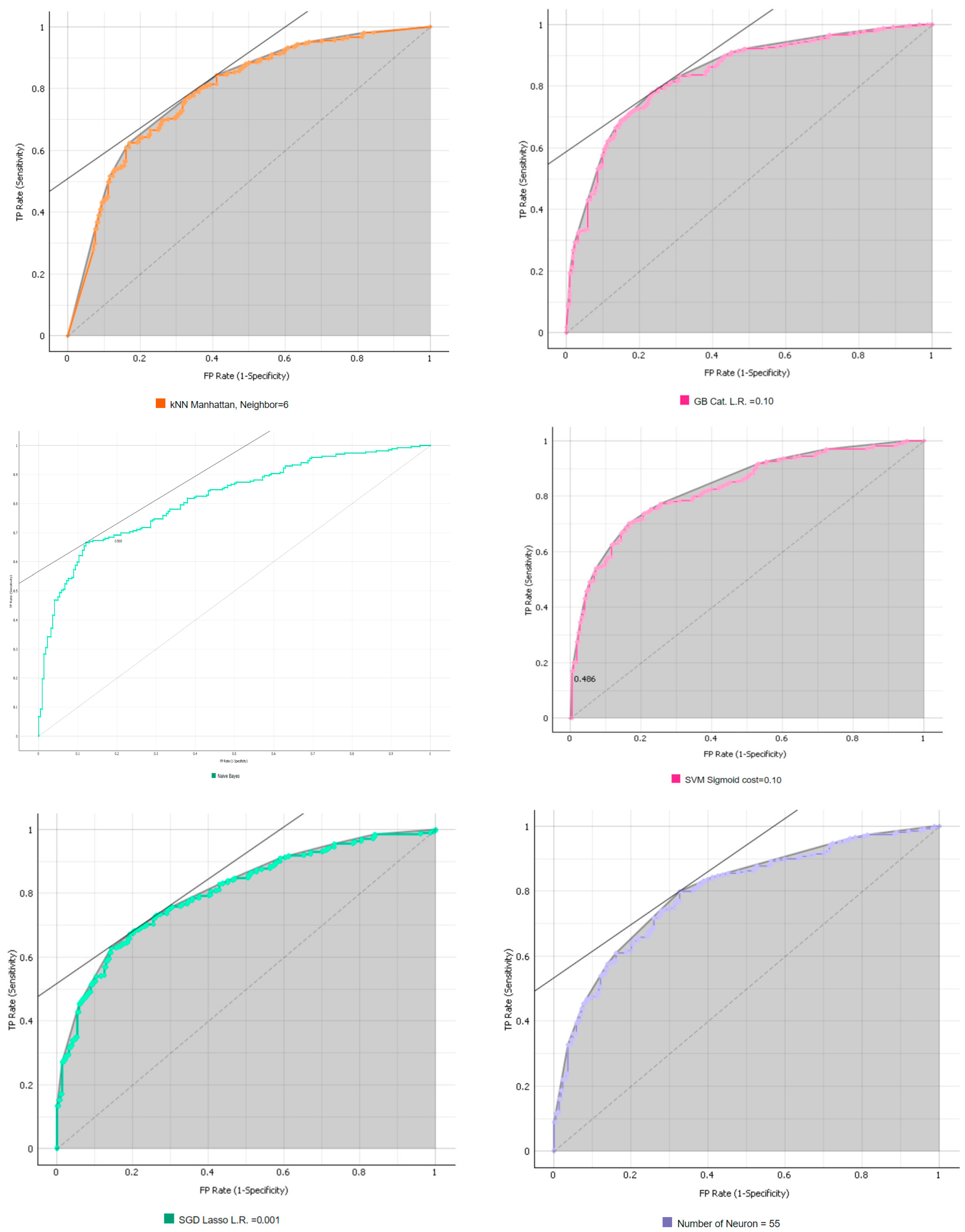
Figure 1. Analytic Structure for the Research (Abbreviations: kNN, k-Nearest Neighbor; NN, Neural Networks; SGD, Stochastic Gradient Descent; SVM, Support Vector Machine).
Mathematics 12 00182 g001
Figure 2. Analytic Process with ML Algorithms and Logistic Regression.
Mathematics 12 00182 g002
Figure 3. ROC Curves from the Best Predictions from Six ML Algorithms.
Mathematics 12 00182 g003
Figure 4. ROC Curves Based on Logistic Regression Modeling.
Mathematics 12 00182 g004
Table 1. Prediction Accuracy Comparison across ML Algorithms.
MLSelected
Algorithm
Selected
Parameter
TrainingTest
kNN Neighbor = 61.0000.844
Gradient BoostingCategorical L.R. = 0.100.9880.849
Naïve Bayes 0.8710.818
SVMSigmoidcost = 0.100.8360.826
SGDLasso/RidgeL.R. = 0.0010.9190.802
NN Neuron = 301.0000.793
Abbreviation: L.R., learning rate.
Table 2. Logistic Regression Results (n = 475, 50% Random Splitting).
VariablesLogistic Regression with
All Variables
Logistic Regression with
Forward Stepwise
Logistic Regression with Backward Stepwise
CoefficientSECoefficientSECoefficientSE
Auto loan0.400.46
Student loan−0.610.47
Farm loan−0.040.80
Equity loan0.220.66
Mortgage loan−1.480.51 −0.69 *0.31
Own house0.500.51
Saving acct.−1.860.51−1.40 ***0.29−1.28 ***0.30
Checking acct.−0.330.57
Term L.I.−0.080.41
Whole L.I.−1.020.51−0.90 **0.33−0.81 *0.34
FA do not know−1.270.64
FA no−1.820.53−1.12 ***0.28−1.14 ***0.28
Payday loan−0.660.56
Health insurance0.610.52
FP Dist. 10 miles0.490.56
FP Dist. 20 miles1.060.61
FP Dist. 50 miles1.080.91
FP Dist. Over 501.401.19
FP Dist. na−0.210.57−0.70 *0.29−0.80 **0.30
Fin course in H.S.−0.810.45−1.01 **0.29−0.95 **0.30
Fin course in Col.−0.470.53
Obj. Fin Knw.−0.080.21
Fin R.T.0.040.05
Fin Satisfaction0.090.040.07 **0.020.06 *0.03
Fin Stress0.020.01
Fin Self-efficacy−0.190.06 −0.08 *0.03
L.O.C.−0.050.05
S.W.L.S.0.080.030.08 ***0.020.08 ***0.02
Self-esteem0.010.05
Job insecurity0.050.04
WS Part-time0.200.71
WS Self-empl.1.310.70
WS Homemaker −1.361.00
WS Full stud.0.280.82
WS Not working0.110.58
Agri. Work0.921.67
Agri. R.Busi.−0.771.02
Agri. No.−0.030.90
Ed AA0.440.50
Ed BA0.930.55
Ed Grad.0.660.74
Single0.220.45
Female0.120.41
Age0.020.02
Suburban0.420.44
Rural0.950.59
Ethn. Hispanic0.160.59
Ethn. Black−0.220.52
Ethn. Asian0.420.55
Ethn. Pacific−0.131.07
Ethn. Others−0.980.87
Inc. 15 k to 25 k−0.710.68
Inc. 25 k to 35 k−1.120.70
Inc. 35 k to 50 k−1.090.73
Inc. 50 k to 75 k−0.270.72
Inc. 75 k to 100 k−0.950.86
Inc. 100 k to 150 k−1.270.85
Inc. > 150 k1.261.27
No. of Child−0.660.20−0.26 *0.12−0.27 *0.12
Hth. Good−0.240.49
Hth. Fair−1.170.68
Hth. Poor0.361.23
Fin Situation−0.480.23−0.32 *0.13
H.Situation−0.100.26
WB.Situation0.030.28
Work. Situation0.320.26
3 months expect−0.310.29
6 months expect0.140.27
1 year expect0.310.25
Stim. May0.580.77
Stim. Jun.−1.240.91
Stim. Jul.0.940.99
Stim. Aft. Jul.−0.740.66
Stim. Dk−0.720.72
Stim. Na−0.621.06
Stim. No get−1.100.74
Stim. No elig.−0.440.81
Constant8.473.903.93 ***1.065.28 ***1.25
R20.54 0.41 0.41
F352.60 264.57 *** 268.99 ***
Note. Reference group for auto loan, student loan, farm loan, equity loan, mortgage loan, own house, saving account, checking account, term life insurance, whole life insurance, financial course from high school, financial course from college are those who do not have them; male is the reference group for gender; ever had financial advice before is the reference group for experience of financial advice; distance to the accessible financial profession within 5 miles is the reference group for accessibility of financial professionals; full-time working status is the reference group for working status; working on a farm is the reference group for agriculture working status; high school or lower degree is the reference group for education level; living in urban area is the reference group for urban/suburban/rural living; lower than USD 15,000 is the reference group for income level; excellent health status is the reference group for health status; reference group for stimulus check is receiving stimulus check in April; the results for region (i.e., states) were omitted because the number of states and territories is too large to report while the sample size per location is too small. Significance level: * p < 0.1, ** p < 0.05, *** p < 0.01.
Table 3. AUC Comparison between ML Algorithms and Logistic Predictions.
MLAUC from TestLogistic RegressionAUC from Test
kNN0.844With all variables0.703
Gradient Boosting0.849Forward stepwise0.741
Naïve Bayes0.818Backward stepwise0.754
SVM0.826
SGD0.802
NN0.793
Table 4. Variable Rankings from Six ML Algorithms.
kNNRFGBRFNaïve BayesRFSVMRFSGDRFNNRF
Accuracy Rank = 2Accuracy Rank = 1Accuracy Rank = 4Accuracy Rank = 3Accuracy Rank = 5Accuracy Rank = 6
1Region0.090Education level0.110Fin Self-efficacy0.075Fin Course in Col.0.176Ever FA0.128Fin Course in Col.0.136
2Equity loan0.080Fin Course in Col.0.104Farm loan0.070Education level0.158Fin Course in Col.0.108Farm loan0.134
3Farm loan0.076Whole L.I.0.102Ever FA0.069Whole L.I.0.158Fin Course in H.S.0.080Ever FA0.117
4Fin Course in Col.0.072Region0.089Checking acct.0.062Farm loan0.144Single0.078Equity loan0.102
5Fin Course in H.S.0.070Ever FA0.079Fin Satisfaction0.057S.W.L.S.0.115Fin Satisfaction0.074Whole L.I.0.088
6Single0.064Farm loan0.062Region0.054Fin Satisfaction0.112Own house0.072Student loan0.086
7Ever FA.0.061Fin Satisfaction0.061Saving acct.0.046Ever FA0.109Gender0.070Payday loan0.082
8Education level0.060Gender0.056S.W.L.S.0.044Fin Stress0.101Farm loan0.068Education level0.080
9S.W.L.S.0.054Single0.054Payday loan0.042Fin Course in H.S.0.092Fin Self-efficacy0.061Fin Satisfaction0.072
10Payday loan0.048Fin Self-efficacy0.053Income level0.040Payday loan0.088S.W.L.S.0.058Term L.I.0.064
11Term L.I.0.040Income level0.051Age0.035Single0.088Fin Stress0.057S.W.L.S.0.055
12Fin Satisfaction0.036Mortgage loan0.0481 year expect0.033Agri. Work. Type0.087Dist. To. FP0.046Agri. Work. Type0.051
13Mortgage loan0.034Fin Stress0.044Fin Stress0.028Fin Self-efficacy0.081Obj. Fin Knw.0.045Auto loan0.048
14Health status0.032Own house0.042Education level0.028Term L.I.0.076Mortgage loan0.044Fin Self-efficacy0.047
15Fin Situation0.031Saving acct.0.040Stimulus0.027Checking acct.0.070Student loan0.040Fin Stress0.046
16Gender0.028Dist. To. FP0.039Fin Course in H.S.0.026Own house0.070Term L.I.0.040Saving acct.0.044
17Auto loan0.028Obj. Fin Knw.0.035WB.Situation0.023Fin Situation0.067Payday loan0.034Single0.038
18Income level0.025Equity loan0.034Equity loan0.022Health status0.066Agri. Work. Type0.033Ethnic0.032
19Fin Self-efficacy0.0236 months expect0.032Dist. To. FP0.021Work status0.065Region0.033WB.Situation0.032
20H.Situation0.023S.W.L.S.0.031Work status0.019Equity loan0.064Job insecurity0.032Fin Course in H.S.0.032
21Student loan0.022Job insecurity0.031Agri. Work. Type0.019H.Situation0.059Equity loan0.032Income0.031
221 year expect0.021Term L.I.0.030L.O.C.0.019WB.Situation0.059Saving acct.0.032Checking acct.0.030
23Urban type0.020Agri. Work. Type0.028Auto loan0.0163 months expect0.055L.O.C.0.031Self-esteem0.028
24Agri. Work. Type0.019Fin Course in H.S.0.0246 months expect0.016L.O.C.0.047Education level0.030Work. Situation0.026
25Self-esteem0.017Ethnic0.024Health status0.015Obj. Fin Knw.0.043Age0.030Region0.026
26Fin Stress0.014Health status0.022Term L.I.0.014Work. Situation0.041WB.Situation0.029Fin Situation0.023
27Saving acct.0.014Payday loan0.022Fin R.T.0.012Stimulus0.040Income level0.026L.O.C.0.023
28Job insecurity0.013Auto loan0.022Obj. Fin Knw.0.011Income level0.040Self-esteem0.025Job insecurity0.021
296 months expect0.013H.Situation0.020Single0.010Health insurance0.040Work status0.024Gender0.020
30Obj. Fin Knw.0.012L.O.C.0.018Urban0.0106 months expect0.039Health status0.023Mortgage loan0.016
31Work status0.010Age0.016H.Situation0.010Job insecurity0.037Urban type0.021Work status0.013
32Age0.0091 year expect0.014Self-esteem0.007Age0.034Health insurance0.016Age0.010
33Ethnic0.008Self-esteem0.012Fin Situation0.007Mortgage loan0.0341 year expect0.015Health status0.009
34Own house0.006No. of Child0.005Own house0.006Self-esteem0.032H.Situation0.014Fin R.T.0.008
35Health insurance0.006Fin R.T.0.005Job insecurity0.003Region0.031Fin Situation0.011H.Situation0.008
36L.O.C.0.005Checking acct.0.004Work. Situation0.003Student loan0.030Checking acct.0.0103 months expect0.007
37Stimulus0.005Fin Situation0.003Student loan0.000Saving acct.0.028Fin R.T.0.009Dist. To. FP0.007
38No. of Child0.003Work. Situation0.000No. of Child−0.001Auto loan0.026Auto loan0.0081 year expect0.001
39Whole L.I.0.000WB.Situation−0.004Ethnic−0.009Dist. To. FP0.010Work. Situation0.008No. of Child0.000
40Fin R.T.−0.0023 months expect−0.0053 months expect−0.010No. of Child0.009Stimulus0.005Own house0.000
41WB. Situation−0.003Health insurance−0.006Gender−0.0121 year expect0.0076 months expect0.004Obj. Fin Knw.−0.002
42Checking acct.−0.012Student loan−0.010Health insurance−0.014Gender0.004Whole L.I.0.004Urban type−0.004
433 months expect−0.025Work status−0.021Mortgage loan−0.018Ethnic−0.002No. of Child−0.004Stimulus−0.005
44Work. Situation−0.029Urban type−0.021Whole L.I.−0.024Fin R.T.−0.004Ethnic−0.013Health insurance−0.014
45Dist. To FP.−0.034Stimulus−0.030Fin Course in Col.−0.024Urban type−0.0193 months expect−0.0206 months expect−0.017
Abbreviations: Agri. Work. Type, agricultural working status; Dist. To. FP, distance to the financial professionals; Ever FA, ever have financial advice; GB, Gradient Boosting; RF, RReliefF; other abbreviations are same as shown in Table 2.
Disclaimer/Publisher’s Note: The statements, opinions and data contained in all publications are solely those of the individual author(s) and contributor(s) and not of MDPI and/or the editor(s). MDPI and/or the editor(s) disclaim responsibility for any injury to people or property resulting from any ideas, methods, instructions or products referred to in the content.

