Figure 1.
Demonstration of the classical RBF. (a) Gaussian RBF; (b) Markoff RBF; (c) Inverse MQ RBF.
Figure 1.
Demonstration of the classical RBF. (a) Gaussian RBF; (b) Markoff RBF; (c) Inverse MQ RBF.
Figure 2.
The results processed by the RBF-assisted part. (a) The coordinates of the center point are . (b) The coordinates of the center point are . (c) The coordinates of the center point are . (d) The coordinates of the center point are .
Figure 2.
The results processed by the RBF-assisted part. (a) The coordinates of the center point are . (b) The coordinates of the center point are . (c) The coordinates of the center point are . (d) The coordinates of the center point are .
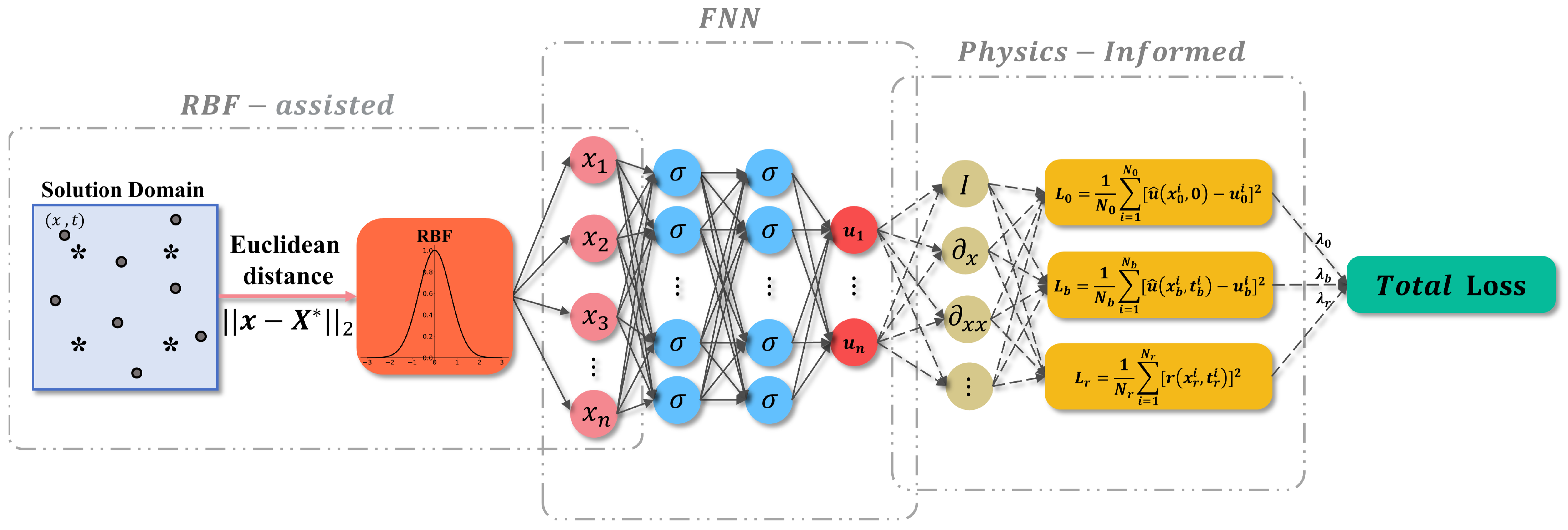
Figure 3.
The architecture of RBF-assisted NN. In the RBF-assisted part, ● denotes the collocation points; * denotes the center points; denotes the coordinate vector of the collocation points; denotes the coordinate vector of the center points.
Figure 3.
The architecture of RBF-assisted NN. In the RBF-assisted part, ● denotes the collocation points; * denotes the center points; denotes the coordinate vector of the collocation points; denotes the coordinate vector of the center points.
Figure 4.
Results of 1D Burgers equation. (a) The predicted solution by PINNs. (b) The absolute error of PINNs. (c) The predicted solution by RBF-assisted NN. (d) The absolute error of RBF-assisted NN.
Figure 4.
Results of 1D Burgers equation. (a) The predicted solution by PINNs. (b) The absolute error of PINNs. (c) The predicted solution by RBF-assisted NN. (d) The absolute error of RBF-assisted NN.
Figure 5.
Comparison of predicted and exact solutions of the 1D Burgers equation for different time snapshots by PINNs. (a) s; (b) s; (c) s; (d) s.
Figure 5.
Comparison of predicted and exact solutions of the 1D Burgers equation for different time snapshots by PINNs. (a) s; (b) s; (c) s; (d) s.
Figure 6.
Comparison of predicted and exact solutions of the 1D Burgers equation for different time snapshots by RBF-assisted NN. (a) s; (b) s; (c) s; (d) s.
Figure 6.
Comparison of predicted and exact solutions of the 1D Burgers equation for different time snapshots by RBF-assisted NN. (a) s; (b) s; (c) s; (d) s.
Figure 7.
Comparison of loss functions between PINNs and RBF-assisted NN with different for the 1D Burgers equation.
Figure 7.
Comparison of loss functions between PINNs and RBF-assisted NN with different for the 1D Burgers equation.
Figure 8.
Results of the 1D Schrodinger equation. (a) The predicted solution by PINNs. (b) The absolute error of PINNs. (c) The predicted solution by RBF-assisted NN. (d) The absolute error of RBF-assisted NN.
Figure 8.
Results of the 1D Schrodinger equation. (a) The predicted solution by PINNs. (b) The absolute error of PINNs. (c) The predicted solution by RBF-assisted NN. (d) The absolute error of RBF-assisted NN.
Figure 9.
Comparison of predicted and exact solutions of the 1D Schrodinger equation for different time snapshots by PINNs. (a) s; (b) s; (c) s; (d) s.
Figure 9.
Comparison of predicted and exact solutions of the 1D Schrodinger equation for different time snapshots by PINNs. (a) s; (b) s; (c) s; (d) s.
Figure 10.
Comparison of predicted and exact solutions of the 1D Schrodinger equation for different time snapshots by RBF-assisted NN. (a) s; (b) s; (c) s; (d) s.
Figure 10.
Comparison of predicted and exact solutions of the 1D Schrodinger equation for different time snapshots by RBF-assisted NN. (a) s; (b) s; (c) s; (d) s.
Figure 11.
Comparison of loss functions between PINNs and RBF-assisted NN with different for the 1D Schrodinger equation.
Figure 11.
Comparison of loss functions between PINNs and RBF-assisted NN with different for the 1D Schrodinger equation.
Figure 12.
Results of the 2D Helmholtz equation. (a) The predicted solution by PINNs. (b) The absolute error of PINNs. (c) The predicted solution by RBF-assisted NN. (d) The absolute error of RBF-assisted NN.
Figure 12.
Results of the 2D Helmholtz equation. (a) The predicted solution by PINNs. (b) The absolute error of PINNs. (c) The predicted solution by RBF-assisted NN. (d) The absolute error of RBF-assisted NN.
Figure 13.
Comparison of predicted and exact solutions of the 2D Helmholtz equation at different space locations by PINNs. (a) ; (b) ; (c) ; (d) .
Figure 13.
Comparison of predicted and exact solutions of the 2D Helmholtz equation at different space locations by PINNs. (a) ; (b) ; (c) ; (d) .
Figure 14.
Comparison of predicted and exact solutions of the 2D Helmholtz equation at different space locations by RBF-assisted NN. (a) ; (b) ; (c) ; (d) .
Figure 14.
Comparison of predicted and exact solutions of the 2D Helmholtz equation at different space locations by RBF-assisted NN. (a) ; (b) ; (c) ; (d) .
Figure 15.
Comparison of loss functions between PINNs and RBF-assisted NN with different for the 2D Helmholtz equation.
Figure 15.
Comparison of loss functions between PINNs and RBF-assisted NN with different for the 2D Helmholtz equation.
Figure 16.
Results of the N–S equation. (a) The predicted solution by PINNs. (b) The absolute error of PINNs. (c) The predicted solution by RBF-assisted NN. (d) The absolute error of RBF-assisted NN.
Figure 16.
Results of the N–S equation. (a) The predicted solution by PINNs. (b) The absolute error of PINNs. (c) The predicted solution by RBF-assisted NN. (d) The absolute error of RBF-assisted NN.
Figure 17.
Comparison of loss functions between PINNs and RBF-assisted NN with different for the N–S equation.
Figure 17.
Comparison of loss functions between PINNs and RBF-assisted NN with different for the N–S equation.
Figure 18.
Results of the N–S equation. (a) The predicted solution by RBF-assisted NN. (b) The solution by the COMSOL.
Figure 18.
Results of the N–S equation. (a) The predicted solution by RBF-assisted NN. (b) The solution by the COMSOL.
Figure 19.
Results of thee Helmholtz equation with a large range solution domain. (a) The predicted solution by PINNs. (b) The predicted solution by RBF-assisted NN (Guassian RBF). (c) The predicted solution by RBF-assisted NN (Maekoff RBF). (d) The predicted solution by RBF-assisted NN (IMQ RBF).
Figure 19.
Results of thee Helmholtz equation with a large range solution domain. (a) The predicted solution by PINNs. (b) The predicted solution by RBF-assisted NN (Guassian RBF). (c) The predicted solution by RBF-assisted NN (Maekoff RBF). (d) The predicted solution by RBF-assisted NN (IMQ RBF).
Figure 20.
Comparison of loss functions between PINNs and RBF-assisted NN with different RBF and different for the Helmholtz equation. (a) Gaussian RBF. (b) Markoff RBF. (c) Inverse MQ RBF.
Figure 20.
Comparison of loss functions between PINNs and RBF-assisted NN with different RBF and different for the Helmholtz equation. (a) Gaussian RBF. (b) Markoff RBF. (c) Inverse MQ RBF.
Table 1.
Three classical radial basis functions.
Table 1.
Three classical radial basis functions.
| RBFs | |
|---|
| Gaussian | |
| Markoff | |
| Inverse MQ (IMQ) | |
Table 2.
Comparison of relative errors and errors between PINNs and RBF-assisted NN with different for the 1D Burgers equation.
Table 2.
Comparison of relative errors and errors between PINNs and RBF-assisted NN with different for the 1D Burgers equation.
| NN Type | | Error | Error |
|---|
| RBF-assisted NN | | | |
| | |
| | |
| | |
| | |
| | |
| PINNs | \ | | 1.050 |
Table 3.
Comparison of relative errors and errors between PINNs and RBF-assisted NN with different for the 1D Schrodinger equation.
Table 3.
Comparison of relative errors and errors between PINNs and RBF-assisted NN with different for the 1D Schrodinger equation.
| NN Type | | Error | Error |
|---|
| RBF-assisted NN | | | |
| | |
| | |
| | |
| | |
| | |
| PINNs | \ | | |
Table 4.
Comparison of relative errors and errors between PINNs and RBF-assisted NN with different for the 2D Helmholtz equation.
Table 4.
Comparison of relative errors and errors between PINNs and RBF-assisted NN with different for the 2D Helmholtz equation.
| NN Type | | Error | Error |
|---|
| RBF-assisted NN | | | |
| | |
| | |
| | |
| | |
| | |
| PINNs | \ | | |
Table 5.
Comparison of relative errors and errors between PINNs and RBF-assisted NN with different RBF shape parameters c for the 2D Helmholtz equation.
Table 5.
Comparison of relative errors and errors between PINNs and RBF-assisted NN with different RBF shape parameters c for the 2D Helmholtz equation.
| Error Type | PINNs | RBF-Assisted NN (c = 0.5) | RBF-Assisted NN (c = 1.0) | RBF-Assisted NN (c = 2.0) |
|---|
| Error | | | | |
| Error | | | | |
Table 6.
Comparison of relative errors and errors between PINNs and RBF-assisted NN with different for the N–S equation.
Table 6.
Comparison of relative errors and errors between PINNs and RBF-assisted NN with different for the N–S equation.
| NN Type | | Error | Error |
|---|
| RBF-assisted NN | | | |
| | |
| | |
| | |
| | |
| | |
| PINNs | \ | | |
Table 7.
Comparison of relative errors and errors between PINNs and RBF-assisted NN with different RBF for the Helmholtz equation.
Table 7.
Comparison of relative errors and errors between PINNs and RBF-assisted NN with different RBF for the Helmholtz equation.
| Error Type | PINNs | RBF-Assisted NN (Gaussian) | RBF-Assisted NN (Markoff) | RBF-Assisted NN (IMQ) |
|---|
| Error | 3.299 | | | |
| Error | 4.516 | | | |
Table 8.
Comparison of relative errors and errors between PINNs and RBF-assisted NN with different RBF and different for the Helmholtz equation.
Table 8.
Comparison of relative errors and errors between PINNs and RBF-assisted NN with different RBF and different for the Helmholtz equation.
| NN Type | | Error | Error |
|---|
| RBF-assisted NN (Gaussian) | | | |
| | |
| | |
| RBF-assisted NN (Markoff) | | | |
| | |
| | |
| RBF-assisted NN (IMQ) | | | |
| | |
| | |
| PINNs | \ | | |


