Abstract
In scientific computing, neural networks have been widely used to solve partial differential equations (PDEs). In this paper, we propose a novel RBF-assisted hybrid neural network for approximating solutions to PDEs. Inspired by the tendency of physics-informed neural networks (PINNs) to become local approximations after training, the proposed method utilizes a radial basis function (RBF) to provide the normalization and localization properties to the input data. The objective of this strategy is to assist the network in solving PDEs more effectively. During the RBF-assisted processing part, the method selects the center points and collocation points separately to effectively manage data size and computational complexity. Subsequently, the RBF processed data are put into the network for predicting the solutions to PDEs. Finally, a series of experiments are conducted to evaluate the novel method. The numerical results confirm that the proposed method can accelerate the convergence speed of the loss function and improve predictive accuracy.
Keywords:
partial differential equations; radial basis function; physics-informed neural networks; numerical solution MSC:
65M99
1. Introduction
Partial differential equations (PDEs) [1,2] are a fundamental tool in scientific research for describing the laws governing the objective physical world. However, analytical solutions of most PDEs may be difficult to obtain. Therefore, it is imperative to explore obtaining approximate numerical solutions. Currently, the primary methods for solving numerical solutions of PDEs include finite volume methods (FVM) [3], finite difference methods (FDM) [4] and finite element methods (FEM) [5]. While these methods are powerful and rigorous, it is important to note that mesh subdivision greatly affects the accuracy of solving PDEs. In addition, the refinement of the grids often results in increased computational complexity and storage costs. These factors limit the practical application of the above methods.
Over the past several years, deep learning has made significant progress in image recognition [6], natural language processing [7], speech recognition [8] and indoor positioning [9]. This progress can be attributed to the rapid growth of high-performance computing resources, algorithmic advancements and improved data accessibility. At the same time, deep learning is famous for its powerful approximation representation and capability of handling nonlinear systems. Therefore, deep learning has been extensively used in scientific computing [10,11,12], especially for solving PDEs. The physics-informed neural networks (PINNs) proposed by Raissi et al. [13] are a significant method in this field. The method transforms the solution of PDEs into the optimization of neural network parameters. This method accurately estimates a physical model from finite data, providing more accurate results for both forward and inverse problems. Owing to their exceptional prediction accuracy and robustness, PINNs have become the benchmark in this field. A series of models have been developed based on their extensions, such as PPINN [14], nPINNs [15], AMAW-PINN [16] and others.
Although PINNs have exhibited remarkable performance in solving PDEs, similar to many deep learning models, they can suffer from training failures or slow convergence. Therefore, further refinements and targeted enhancements [17] are necessary to improve their adaptability, accuracy, computational efficiency and generalization for specific problems. Jagtap et al. [18,19] introduced learnable parameters in the activation function to adaptively control the learning rate of PINNs. This method not only accelerates the convergence of neural networks, but also improves the robustness and accuracy of the neural network approximation. Wang et al. [20] proposed an adaptive hyper-parameter selection algorithm that accelerates the convergence speed of PINNs and improves their prediction accuracy. Furthermore, Sivalingam et al. [21,22] introduced TFC (Theory of Functional Connection) to construct constrained expressions to solve the problem of PINNs failing to satisfy the initial conditions analytically. At the same time, scholars have explored the combination of PINNs with various network structures, such as Long Short-term Memory Networks (LSTM), Convolutional Neural Networks (CNN), Generative Adversarial Networks (GAN) and Bayesian networks, to solve different equations. Several studies have been conducted in this area, including PI-GAN [23], B-PINN [24], Resnet-PINN [25] and TgAE-PINN [26].
Although traditional numerical methods have some drawbacks, their stability and interpretability have attracted many scholars to combine them with neural networks for solving PDEs. Ramuhalli et al. [27] and Mitusch et al. [28] proposed the FENN model and the FEM-NN model based on finite element methods, respectively. Shi et al. [29] proposed a neural network named FD-Net, which employs finite difference methods to learn partial derivatives and learns the governing PDEs from trajectory data. Praditia et al. [30] proposed the FINN by combining deep learning with finite volume methods. The method can accurately handle various types of numerical boundary conditions by effectively managing the fluxes between control volumes. Furthermore, Li et al. [31] proposed the DWNN, which combines wavelet transform with neural networks. The method utilized wavelets to obtain a detailed description of the features, which improves the prediction accuracy of the equations. Ramabathiran et al. [32] combined a meshless method with neural networks and proposed a sparse deep neural network called SPINN. This method enhances the interpretability of neural networks for solving PDEs. Additionally, the neural tangent kernel [33] (NTK) has been introduced into the study of PINNs. Bai et al. [34] analyzed the training dynamics of PINNs with the help of NTK theory and observed that PINNs tend to be local approximators after training.
Motivated by the above studies, we propose an RBF-assisted hybrid neural network (RBF-assisted NN) that combines neural networks with a radial basis function (RBF) to approximate solutions of PDEs. As PINNs tend to become a local approximator [34] after training, the proposed method utilizes RBF to provide the normalization and localization properties to the input data. By providing the normalization property to the input data, the proposed method is able to directly solve the large range solution domain problems. At the same time, by providing the localization property for the input data, the proposed method can make the network model become a local approximator more quickly. In the RBF-assisted processing part, we adopted the method proposed by Chen et al. [35] to select the center points and collocation points separately. This method can help the RBF-assisted NN to effectively manage data size and computational complexity. Subsequently, the RBF processed data are put into the network for predicting the solutions to PDEs. Finally, the effectiveness of the method is evaluated by several numerical experiments to verify its performance in solving PDEs.
The paper is structured as follows: Section 2 provides a brief overview of PINNs, followed by a detailed introduction to the RBF-assisted part. Subsequently, the structure of the network is described, and a procedure for using the network to solve PDEs is provided. Section 3 validates the effectiveness of the novel method through several numerical experiments. Finally, Section 4 and Section 5 present the discussion and conclusions of the paper.
2. Methodology
2.1. Overview of PINNs
In this section, we will give a brief overview of PINNs [13]. Before that, we consider a PDE of the general form in a bounded domain :
where u is the solution of the Equation (1), and is the differential operator; denotes the initial condition, and denotes the Neumann, Dirichlet or mixed boundary conditions. The objective of the equation is to obtain the solution u under the given initial and boundary conditions.
In PINNs, fully connected neural networks are commonly used to approximate the solution of the PDEs. The neural network architecture usually consists of an input layer, hidden layers and an output layer. The neural network takes the input of space and time coordinates and outputs an approximation of the solution to the PDEs. Assuming that the output vector of the ith hidden layer is , the neural network can be represented as:
where denotes the input layer, denotes the output vector of the hidden layers and denotes the approximation u of the equation. denotes the nonlinear activation function. and denote the weight matrix and bias vector of the ith hidden layer, which are the parameters that need to be optimized during model training.
PINNs use deep neural networks to approximate the solutions of the equations. The residuals of the governing equations are defined as:
The essence of PINNs is to add equations (i.e., residuals) to the training of the network as the physical constraints. Therefore, the loss function is in a general form:
where denotes the loss of the governing equations; denotes the loss of the initial conditions; denotes the loss of the boundary conditions. denotes the parameters of the neural network. During the training process, PINNs optimize the parameters and using gradient descent to minimize the loss function. This enables the network to learn the solution that best matches the known physical information.
2.2. RBF-Assisted Part
In this section, we initially give a brief explanation to the properties of the RBF and then describe the computation process of the RBF-assisted part.
Unlike classical basis functions, the radial basis function [36] (RBF) is a function of the distance between data points, i.e., , where represents the RBF. Table 1 presents three classical radial basis functions [37].

Table 1.
Three classical radial basis functions.
To illustrate the properties of different RBFs, we have plotted the function of the RBF described in Table 1. The results are shown in Figure 1.
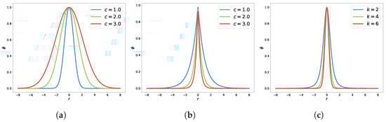
Figure 1.
Demonstration of the classical RBF. (a) Gaussian RBF; (b) Markoff RBF; (c) Inverse MQ RBF.
By examining the function plot of the RBF, two properties can be summarized:
- (1)
- The RBF values are between , which indicates that the data have been normalized after RBF processing. In this paper, we refer to this feature as the normalization property.
- (2)
- The RBF values have a large function value only when the distance r between the data points is small. As the distance r increases, the RBF values tend to decrease monotonically. In this paper, we refer to this feature as the localization property.
Building on the properties of RBF above, we use RBF to process the input data (i.e., the coordinate values of data points) for the neural network. This processing ensures that the data put into the neural network exhibits the normalization and localization properties.
Traditionally, the RBF methods take the center point and collocation point to be the same [38,39,40], resulting in a relatively large size of distance matrix. Therefore, we adopt the method proposed by Chen et al. [35], in which the center points and collocation points are selected separately in the solution domain. Not only can this method effectively control the size of the function values after RBF processing, but it can also save the use of computational resources.
Subsequently, we will use a two-dimensional space to illustrate how the RBF-assisted part works. First of all, M collocation points and N center points are selected within the solution domain . Then, the distance matrix between the collocation points and the center points is computed using the following formula:
By taking the distance matrix into the RBF , we obtain the data processed by the RBF-assisted part. In order to visually demonstrate the properties of the processed data, we selected four center points in the region and plotted the results of the collocation points after processing through the RBF-assisted part. Figure 2 shows that the function values range between , with larger values concentrated around the center points. As the distance from the center points increases, the function values gradually approach zero.
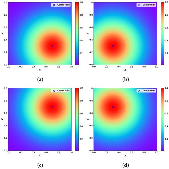
Figure 2.
The results processed by the RBF-assisted part. (a) The coordinates of the center point are . (b) The coordinates of the center point are . (c) The coordinates of the center point are . (d) The coordinates of the center point are .
2.3. Architecture of RBF-Assisted NN
In this section, we propose an RBF-assisted hybrid neural network (RBF-assisted NN) for approximating solutions to PDEs. The proposed model is an extension of the PINNs. It utilizes RBF to assist in processing the input data, providing the normalization and localization properties to the input data. The architecture of the model is shown in Figure 3.
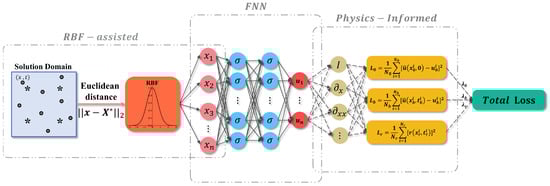
Figure 3.
The architecture of RBF-assisted NN. In the RBF-assisted part, ● denotes the collocation points; * denotes the center points; denotes the coordinate vector of the collocation points; denotes the coordinate vector of the center points.
As shown in Figure 3, the proposed model consists of two parts: an RBF-assisted part and a fully connected neural network (FNN) part. In the RBF-assisted part, there are m collocation points and n center points in the solution domain . The distance matrix between the collocation points and the center points can be calculated by Equation (9). Subsequently, the distance matrix is processed using RBF to obtain the input data of the FNN. Therefore, the number of neurons in the input layer of the FNN should be set to match the number of center points.
In the FNN part, we define the approximation obtained by the network as . At the same time, the residual term of the governing equation is defined as , and its specific expression is given below:
The above residual terms can be obtained by using the AD module in the Pytorch [41] framework. Thus, the loss function expression for the FNN is as follows:
where , and are the weight values for the loss functions (in this paper, these are set to 1.0); denotes the residuals loss term; denotes the initial conditions loss term; denotes the boundary conditions loss term. The specific definitions of the above loss terms are as follows:
Here, denotes the residual points, denotes the initial points and denotes the boundary points. and denote the reference values corresponding to the initial points and the boundary points. denotes the number of residual points, denotes the number of initial points and denotes the number of boundary points. It should be noted that the collocation points consist of residual points, initial points and boundary points combined. After preparing the training data, the neural network is optimized using gradient descent methods to minimize the loss function. In Algorithm 1, the specific steps for the implementation of the proposed method are presented.
| Algorithm 1 RBF-Assisted Hybrid Neural Network for Solving Partial Differential Equations |
| Require: Number of initial points ; Number of boundary points ; Number of residual points ; Center points ; Ensure: Neural network predicted solution .
|
3. Numerical Experiments
In this section, we demonstrate the validity and robustness of the proposed method by several experiments: the 1D Burgers equation, the 1D Schrodinger equation, the 2D Helmholtz equation and the flow in a lid-driven cavity. Subsequently, we also compared the effects of different RBF on the RBF-assisted NN. Throughout the experimental stage, we use the relative error and error to evaluate the accuracy of the numerical solution. Concurrently, the NVIDIA RTX A5000 GPU with 24 GB of memory was utilized to complete all experiments. The results indicate that the proposed method accelerates the convergence of the loss function and enhances the predictive accuracy.
3.1. 1D Burgers Equation
In 1915, Bateman proposed the Burgers equation [42] for the study of fluid motion. The model has played a significant role in different fields, including fluid dynamics, quantum field theory and communication technology. Therefore, it is important to explore the numerical solution of the Burgers equation. In this section, we consider the 1D Burgers equation under the Dirichlet BCs. The specific expression of the equation is as follows:
where u denotes the solution of the equation; t denotes time and x denotes spatial coordinates. denotes the initial condition; and denote the boundary conditions. is set to in this paper.
For this PDE, the residual term is set as follows:
Correspondingly, the loss function of the Burgers equation is expressed as:
where
In the RBF-assisted part, a Gaussian RBF with a shape parameter of was chosen as the basis function. And a total of points were uniformly selected from the solution domain to form the center points . The neural network in the experiment consists of five hidden layers, with each layer containing twenty neurons. The activation function of the network is the Tanh function. The training data for the network consist of the residual points, the initial points and the boundary points, which, together, form the collocation points . During the training process, the number of residual points is set to , the number of initial points is set to and the number of boundary points is set to . The training process employs both the Adam optimizer and the L-BFGS optimizer to jointly optimize the loss function. The Adam optimizer learning rate is set to . The experimental results were obtained after 100 iterations of Adam training and 20,000 iterations of L-BFGS training. Concurrently, as a comparative methodology, the parameter configurations of PINNs are consistent with the aforementioned parameters.
Figure 4 illustrates the predicted solutions and the absolute errors for the Burgers equation. Although both methods can successfully solve the Burgers equation, the RBF-assisted NN has a smaller absolute error compared to the PINNs. In order to better compare the predicted solutions of the two methods, we have plotted their results at four different times (t = 0.3 s, t = 0.5 s, t = 0.7 s and t = 0.9 s). Figure 5 illustrates the results for PINNs, while Figure 6 illustrates the results for RBF-assisted NN. The exact solution of the Burgers equation is represented by the black solid line, while the predicted solution of the network model is represented by the magenta dashed line. The results show that the predicted solutions of RBF-assisted NN are closer to exact solutions than PINNs at two times: t = 0.7 s and t = 0.9 s.
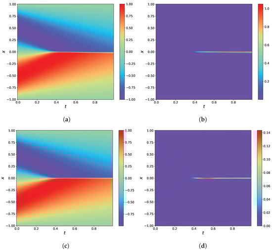
Figure 4.
Results of 1D Burgers equation. (a) The predicted solution by PINNs. (b) The absolute error of PINNs. (c) The predicted solution by RBF-assisted NN. (d) The absolute error of RBF-assisted NN.
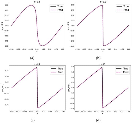
Figure 5.
Comparison of predicted and exact solutions of the 1D Burgers equation for different time snapshots by PINNs. (a) s; (b) s; (c) s; (d) s.
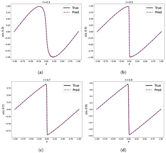
Figure 6.
Comparison of predicted and exact solutions of the 1D Burgers equation for different time snapshots by RBF-assisted NN. (a) s; (b) s; (c) s; (d) s.
In order to compare the effect of a different number of center points (i.e., ) on the results, we uniformly selected different numbers of center points within the solution domain. The experimental results are summarized in Table 2. Comparing the data presented in Table 2, it can be seen that the RBF-assisted NN has the highest solution accuracy when the number of center points is set to 25. Meanwhile, the experimental results of RBF-assisted NN compared to PINNs are better in all cases, regardless of the number of center points used. Figure 7 illustrates the difference in loss function between PINNs and RBF-assisted NN for different numbers of center points. The loss function evolution in Figure 7 indicates that RBF-assisted NN converge faster than PINNs.
Table 2.
Comparison of relative errors and errors between PINNs and RBF-assisted NN with different for the 1D Burgers equation.
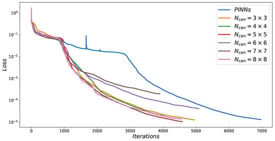
Figure 7.
Comparison of loss functions between PINNs and RBF-assisted NN with different for the 1D Burgers equation.
3.2. 1D Schrodinger Equation
The Schrodinger equation [43] is one of the most important equations of quantum mechanics, which exposes the fundamental laws of the microphysical world. In this section, we consider the 1D Schrodinger equation under the Dirichlet and Neumann mixed BCs. The specific expression of the equation is as follows:
where t denotes time and x denotes spatial coordinates. denotes the initial condition; , , and denote the boundary conditions. denotes the solution of the equation, which consists of a real part u and imaginary part v. Therefore, the solution can be written as . And Equation (21) is reformulated as:
For this PDE, the residual term is set as follows:
Correspondingly, the loss function of the Schrodinger equation is expressed as:
where
In the RBF-assisted part, an Inverse MQ RBF with a shape parameter of was chosen as the basis function. And a total of points were uniformly selected from the solution domain to form the center points . The neural network in the experiment consists of three hidden layers, with each layer containing twelve neurons. The activation function of the network is the Tanh function. The training data for the network consist of the residual points, the initial points and the boundary points, which, together, form the collocation points . During the training process, the number of residual points is set to , the number of initial points is set to and the number of boundary points is set to . The training process employs both the Adam optimizer and the L-BFGS optimizer to jointly optimize the loss function. The Adam optimizer learning rate is set to . The experimental results were obtained after 100 iterations of Adam training and 20,000 iterations of L-BFGS training. Concurrently, as a comparative methodology, the parameter configurations of PINNs are consistent with the aforementioned parameters.
Figure 8 illustrates the predicted solutions and the absolute errors for the Schrodinger equation. While both methods successfully solve the Schrodinger equation, the RBF-assisted NN exhibits a smaller absolute error compared to PINNs. In order to better compare the predicted solutions of the two methods, we have plotted the results at four different times ( s, s, s and s). Figure 9 illustrates the results for PINNs, while Figure 10 illustrates the results for RBF-assisted NN. The exact solution of the Schrodinger equation is represented by the black solid line, while the predicted solution of the network model is represented by the magenta dashed line. Comparing the function plots at the four specified times, it is clear that the predicted RBF-assisted NN solutions are much closer to the exact solutions than PINNs.
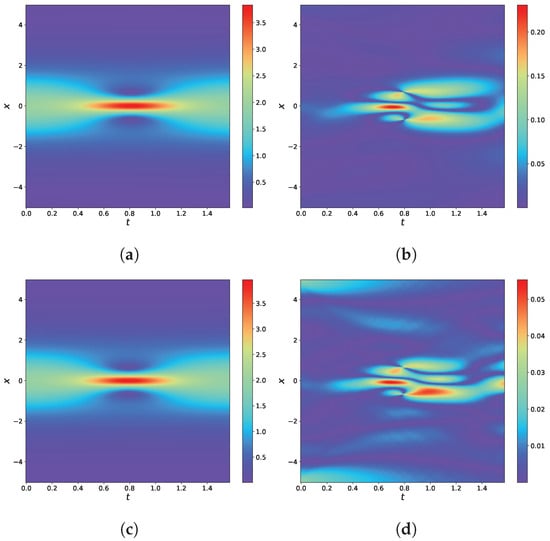
Figure 8.
Results of the 1D Schrodinger equation. (a) The predicted solution by PINNs. (b) The absolute error of PINNs. (c) The predicted solution by RBF-assisted NN. (d) The absolute error of RBF-assisted NN.
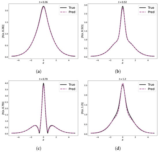
Figure 9.
Comparison of predicted and exact solutions of the 1D Schrodinger equation for different time snapshots by PINNs. (a) s; (b) s; (c) s; (d) s.
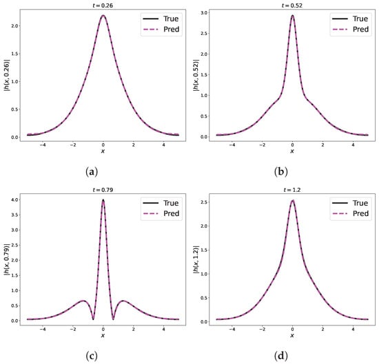
Figure 10.
Comparison of predicted and exact solutions of the 1D Schrodinger equation for different time snapshots by RBF-assisted NN. (a) s; (b) s; (c) s; (d) s.
Similar to the previous experiment, in order to compare the effect of a different number of center points (i.e., ) on the results, we also chose different numbers of center points uniformly within the solution domain. The experimental results are summarized in Table 3. Comparing the data presented in Table 3, it can be seen that the RBF-assisted NN has the highest solution accuracy when the number of center points is set to 36. Meanwhile, regardless of the number of center points used, the experimental results of RBF-assisted NN are slightly better than PINNs in all cases. Similarly, Figure 11 illustrates the difference in loss function between PINNs and RBF-assisted NN for different numbers of center points. The loss function evolution in Figure 11 indicates that RBF-assisted NN converge slightly faster than PINNs.
Table 3.
Comparison of relative errors and errors between PINNs and RBF-assisted NN with different for the 1D Schrodinger equation.
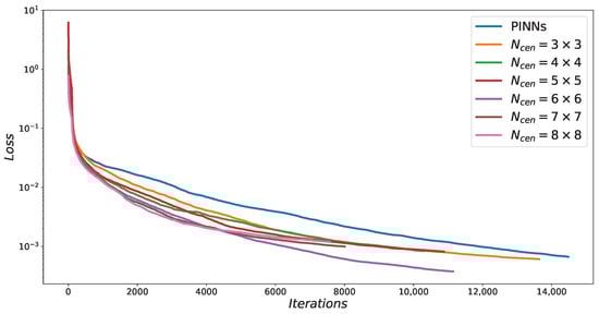
Figure 11.
Comparison of loss functions between PINNs and RBF-assisted NN with different for the 1D Schrodinger equation.
3.3. 2D Helmholtz Equation
The Helmholtz equation is an important class of physical equations that describes various wave phenomena in the real world. The equation is commonly used in a number of fields, including: electromagnetism [44], acoustics [45], geophysics [46] and other sciences. In this section, we consider the 2D Helmholtz equation under the Dirichlet BCs. The specific expression of the equation is as follows:
where u denotes the solution of the equation; x and y denote spatial coordinates; k is a constant value (k is set to 1.0 in this paper). denotes the source term, and denotes the boundary conditions.
For this equation, the source term is given by:
where and are equation parameters ( and are set to 2 in this paper), so the corresponding exact solution expression is as follows:
For this PDE, the residual term is set as follows:
Correspondingly, the loss function of the Helmholtz equation is expressed as:
where
In the RBF-assisted part, a Gaussian RBF with a shape parameter of was chosen as the basis function. And a total of points were uniformly selected from the solution domain to form the center points . The neural network in the experiment consists of five hidden layers, with each layer containing twenty neurons. The activation function of the network is the Tanh function. The training data for the network consist of the residual points and the boundary points, which, together, form the collocation points . During the training process, the number of residual points is set to = 10,000 and the number of boundary points is set to . The training process employs both the Adam optimizer and the L-BFGS optimizer to jointly optimize the loss function. The Adam optimizer learning rate is set to . The experimental results were obtained after 200 iterations of Adam training and 20,000 iterations of L-BFGS training. Concurrently, as a comparative methodology, the parameter configurations of PINNs are consistent with the aforementioned parameters.
Figure 12 illustrates the predicted solutions and the absolute errors for the Helmholtz equation. Although both methods can successfully solve the Helmholtz equation, the RBF-assisted NN exhibits a smaller absolute error compared to the PINNs. In order to better compare the predicted solutions of the two methods, we have plotted their results at four different locations (, , and ). Figure 13 illustrates the results for PINNs, while Figure 14 illustrates the results for RBF-assisted NN. The exact solution of the Helmholtz equation is represented by the black solid line, while the predicted solution of the network model is represented by the magenta dashed line. By examining the function plots at different positions, it is evident that both the PINNs and the RBF-assisted NN are very close to the exact solutions. It can be a challenge to distinguish between the two methods.
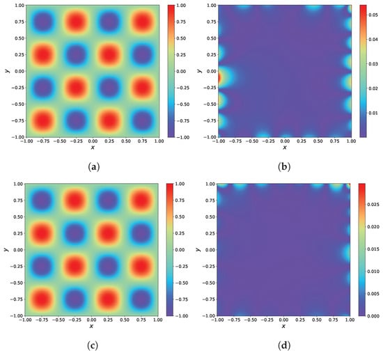
Figure 12.
Results of the 2D Helmholtz equation. (a) The predicted solution by PINNs. (b) The absolute error of PINNs. (c) The predicted solution by RBF-assisted NN. (d) The absolute error of RBF-assisted NN.
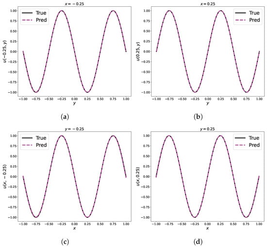
Figure 13.
Comparison of predicted and exact solutions of the 2D Helmholtz equation at different space locations by PINNs. (a) ; (b) ; (c) ; (d) .
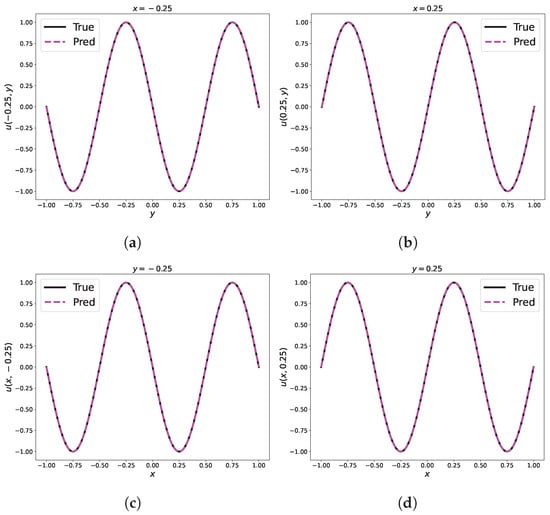
Figure 14.
Comparison of predicted and exact solutions of the 2D Helmholtz equation at different space locations by RBF-assisted NN. (a) ; (b) ; (c) ; (d) .
Similar to the previous experiment, in order to compare the effect of a different number of center points (i.e., ) on the results, we also chose different numbers of center points uniformly within the solution domain. The experimental results are summarized in Table 4. Comparing the data presented in Table 4, it can be seen that the RBF-assisted NN has the highest solution accuracy when the number of center points is set to 25. Meanwhile, regardless of the number of center points used, the experimental results of RBF-assisted NN are significantly better than PINNs in all cases. Similarly, Figure 15 illustrates the difference in loss function between PINNs and RBF-assisted NN for different numbers of center points. The loss function evolution in Figure 15 indicates that RBF-assisted NN converge faster than PINNs.
Table 4.
Comparison of relative errors and errors between PINNs and RBF-assisted NN with different for the 2D Helmholtz equation.
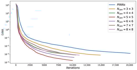
Figure 15.
Comparison of loss functions between PINNs and RBF-assisted NN with different for the 2D Helmholtz equation.
Finally, in order to compare the influence of the shape parameter c on the results, we conducted an experiment with different values of c. In this experiment, the shape parameter c was set to 0.5, 1.0 and 2.0, and the experimental results are summarized in Table 5. The data in Table 5 show that RBF-assisted NN with different shape parameters c are able to improve the accuracy of solving the equations compared to PINNs.
Table 5.
Comparison of relative errors and errors between PINNs and RBF-assisted NN with different RBF shape parameters c for the 2D Helmholtz equation.
3.4. Flow in a Lid-Driven Cavity
In this section, we consider a typical flow problem in fluid dynamics: the flow in a lid-driven cavity. In this problem, the top lid moves at a constant velocity in a closed square container, while the other three boundaries are solid walls. The motion of the top lid drives the fluid motion inside the square cavity, forming a complex vortex. The system is governed by the incompressible Navier–Stokes equations; the specific expression for the the flow in a lid-driven cavity [47] is as follows:
where x and y denote spatial coordinates; denotes the Reynolds number ( is set to 100 in this paper). denotes the solution domain ( is set to in this paper). denotes the top boundary, and denotes the other three boundaries. All four boundaries are subject to the Dirichlet BCs. p denotes the pressure, and denotes the solution of the equation, which consists of the velocity component in the x-direction and the velocity component in the y-direction . Therefore, the solution can be written as . And Equation (36) is reformulated as:
For this PDE, the residual term is set as follows:
Correspondingly, the loss function of the N–S equation is expressed as:
where
In the RBF-assisted part, a Gaussian RBF with a shape parameter of was chosen as the basis function. And a total of points were uniformly selected from the solution domain to form the center points . The neural network in the experiment consists of four hidden layers, with each layer containing twenty neurons. The activation function of the network is the Tanh function. The training data for the network consist of the residual points and the boundary points, which, together, form the collocation points . During the training process, the number of residual points is set to and the number of boundary points is set to . The training process employs both the Adam optimizer and the L-BFGS optimizer to jointly optimize the loss function. The Adam optimizer learning rate is set to . The experimental results were obtained after 1000 iterations of Adam training and 20,000 iterations of L-BFGS training. Concurrently, as a comparative methodology, the parameter configurations of PINNs are consistent with the aforementioned parameters.
Figure 16 illustrates the predicted solutions and the absolute errors for the N–S equation. As shown in Figure 16, RBF-assisted NN can solve the flow in a lid-driven cavity problem more efficiently than PINNs.
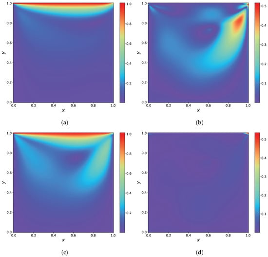
Figure 16.
Results of the N–S equation. (a) The predicted solution by PINNs. (b) The absolute error of PINNs. (c) The predicted solution by RBF-assisted NN. (d) The absolute error of RBF-assisted NN.
Similar to the previous experiment, in order to compare the effect of a different number of center points (i.e., ) on the results, we also chose different numbers of center points uniformly within the solution domain. The experimental results are summarized in Table 6. Comparing the data presented in Table 6, it can be seen that the RBF-assisted NN has the highest solution accuracy when the number of center points is set to 64. Meanwhile, regardless of the number of center points used, the experimental results of RBF-assisted NN are also significantly better than PINNs in all cases. Similarly, Figure 17 illustrates the difference in loss function between PINNs and RBF-assisted NN for different numbers of center points. The evolution of the loss function depicted in Figure 17 indicates that the RBF-assisted NN converges slightly faster than the PINNs and achieves lower loss values.
Table 6.
Comparison of relative errors and errors between PINNs and RBF-assisted NN with different for the N–S equation.
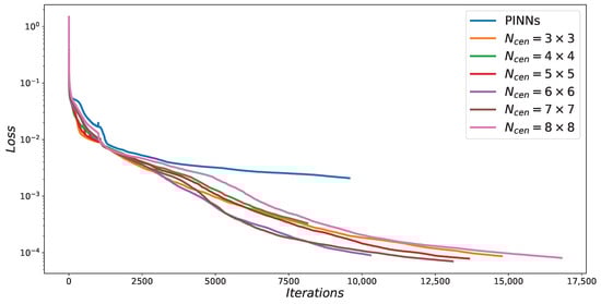
Figure 17.
Comparison of loss functions between PINNs and RBF-assisted NN with different for the N–S equation.
Finally, the flow in a lid-driven cavity problem is simulated using the COMSOL 5.6 software (a finite element analysis software), and the experimental results are shown in Figure 18. By comparing the results, we find that the result of RBF-assisted NN is basically consistent with the result of the COMSOL. This further validates the effectiveness of the RBF-assisted NN in solving the flow in a lid-driven cavity problem.
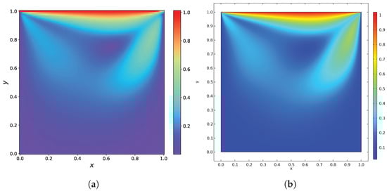
Figure 18.
Results of the N–S equation. (a) The predicted solution by RBF-assisted NN. (b) The solution by the COMSOL.
3.5. Comparative Analysis of RBF-Assisted NN Using Different RBF
In this section, we utilize the 2D Helmholtz equation to verify the normalization property of RBF and to assess the effect of different RBF on the RBF-assisted NN.
Firstly, the normalization property of the RBF is verified by extending the solution domain of Equation (29) from to . The residual points are set to 40,000, the boundary points are set to 800 and the number of center points is set to 64, while the rest of the settings are kept the same as in Section 3.3. Figure 19 shows the results of the experiments. As shown in Figure 19, the PINNs are unable to solve the large range solution domain efficiently, while the RBF-assisted NN can solve it successfully. These results demonstrate that the RBF can provide the normalization property to the data, so the input data to the RBF-assisted NN do not require prior normalization. Subsequently, the errors of PINNs and RBF-assisted NN are compared by using three different RBF to solve the 2D Helmholtz equation. And the results are shown in Table 7.
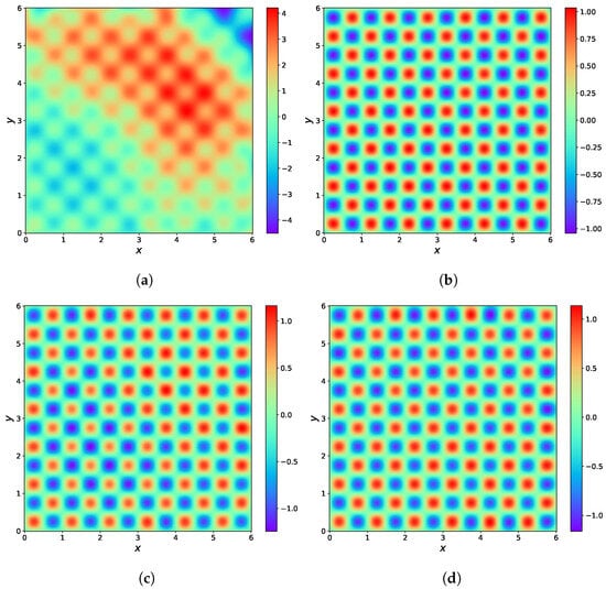
Figure 19.
Results of thee Helmholtz equation with a large range solution domain. (a) The predicted solution by PINNs. (b) The predicted solution by RBF-assisted NN (Guassian RBF). (c) The predicted solution by RBF-assisted NN (Maekoff RBF). (d) The predicted solution by RBF-assisted NN (IMQ RBF).
Table 7.
Comparison of relative errors and errors between PINNs and RBF-assisted NN with different RBF for the Helmholtz equation.
Finally, we compared the effects of different RBF on the RBF-assisted NN. For this experiment, we only modified the RBF used in the RBF-assisted NN. The other settings remained the same as in Section 3.3. The experimental results are shown in Figure 20 and Table 8. A comparison of the experimental results indicates that employing different RBF can improve predictive accuracy. Furthermore, except for the Markoff RBF, utilizing the remaining two RBF can speed up the convergence of the loss function.
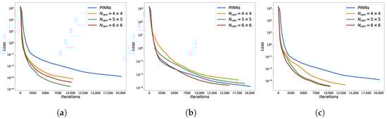
Figure 20.
Comparison of loss functions between PINNs and RBF-assisted NN with different RBF and different for the Helmholtz equation. (a) Gaussian RBF. (b) Markoff RBF. (c) Inverse MQ RBF.
Table 8.
Comparison of relative errors and errors between PINNs and RBF-assisted NN with different RBF and different for the Helmholtz equation.
4. Discussion
In this work, we proposed an RBF-assisted hybrid neural network for approximating solutions to PDEs. The proposed method utilizes RBF to provide the normalization and localization properties to the input data. The experimental results show that the proposed method can accelerate the convergence of the loss function and enhances the predictive accuracy. However, it should be noted that the method has one limitation: the parameters of RBF must be manually selected prior to training. In the future, we intend to set the parameters of the RBF as learnable parameters so that the network model can automatically select more suitable parameters.
5. Conclusions
In this paper, a novel RBF-assisted hybrid neural network is proposed for the approximation of solutions to PDEs. Motivated by the tendency of PINNs to become a local approximator after training, the proposed method utilizes RBF to provide the normalization and localization properties to the input data. By providing the normalization property to the input data, the proposed method is able to directly solve large range solution domain problems. At the same time, by providing the localization property for the input data, the proposed method can make the network model become a local approximator more quickly. During the RBF-assisted processing part, the method selects the center points and collocation points separately to effectively manage data size and computational complexity. Subsequently, the RBF processed data are put into the network for predicting the solutions to PDEs. In order to validate the effectiveness of the proposed method, we analyze its performance through a series of experiments. Subsequently, we also compared the effects of different RBF on the RBF-assisted NN. The results indicate that the proposed method accelerates the convergence of the loss function and enhances the predictive accuracy.
Author Contributions
Conceptualization, Y.L. and S.Y.; methodology, Y.L. and W.G.; software, W.G.; writing—original draft preparation, W.G.; writing—review and editing, Y.L. and S.Y.; visualization, W.G.; supervision, Y.L. and S.Y.; funding acquisition, Y.L. and S.Y. All authors have read and agreed to the published version of the manuscript.
Funding
This research was funded by the National Key Research and Development Program of China (No. 2021YFA1003004 and No. 2023YFC2507500).
Data Availability Statement
The data will be made available by the authors on request.
Conflicts of Interest
The authors declare no conflicts of interest.
Abbreviations
The following abbreviations are used in this manuscript:
| PDEs | Partial Differential Equations |
| FVM | Finite Volume Method |
| FDM | Finite Difference Method |
| FEM | Finite Element Method |
| PINNs | Physics-Informed Neural Networks |
| LSTM | Long Short-Term Memory |
| CNN | Convolutional Neural Network |
| GAN | Generative Adversial Network |
| RBF | Radial Basis Function |
| NTK | Neural Tangent Kernel |
| DWNN | Deep Wavelet Neural Network |
References
- Renardy, M.; Rogers, R.C. An Introduction to Partial Differential Equations; Springer Science & Business Media: Berlin/Heidelberg, Germany, 2006; Volume 13. [Google Scholar]
- Olver, P.J. Introduction to Partial Differential Equations; Springer: Berlin/Heidelberg, Germany, 2014; Volume 1. [Google Scholar]
- Eymard, R.; Gallouët, T.; Herbin, R. Finite volume methods. Handb. Numer. Anal. 2000, 7, 713–1018. [Google Scholar] [CrossRef]
- Thomas, J.W. Numerical Partial Differential Equations: Finite Difference Methods; Springer Science & Business Media: Berlin/Heidelberg, Germany, 2013; Volume 22. [Google Scholar]
- Taylor, C.A.; Hughes, T.J.; Zarins, C.K. Finite element modeling of blood flow in arteries. Comput. Methods Appl. Mech. Eng. 1998, 158, 155–196. [Google Scholar] [CrossRef]
- Traore, B.B.; Kamsu-Foguem, B.; Tangara, F. Deep convolution neural network for image recognition. Ecol. Inform. 2018, 48, 257–268. [Google Scholar] [CrossRef]
- Goldberg, Y. Neural Network Methods for Natural Language Processing; Springer: Berlin/Heidelberg, Germany, 2022. [Google Scholar]
- Abdel-Hamid, O.; Mohamed, A.R.; Jiang, H.; Deng, L.; Penn, G.; Yu, D. Convolutional neural networks for speech recognition. IEEE/ACM Trans. Audio Speech Lang. Process. 2014, 22, 1533–1545. [Google Scholar] [CrossRef]
- Fei, R.; Guo, Y.; Li, J.; Hu, B.; Yang, L. An improved BPNN method based on probability density for indoor location. IEICE Trans. Inf. Syst. 2023, 106, 773–785. [Google Scholar] [CrossRef]
- Az-Zo’bi, E.A.; Shah, R.; Alyousef, H.A.; Tiofack, C.; El-Tantawy, S. On the feed-forward neural network for analyzing pantograph equations. AIP Adv. 2024, 14, 025042. [Google Scholar] [CrossRef]
- Zheng, Y.; Wang, Y.; Liu, J. Research on structure optimization and motion characteristics of wearable medical robotics based on improved particle swarm optimization algorithm. Future Gener. Comput. Syst. 2022, 129, 187–198. [Google Scholar] [CrossRef]
- Ruttanaprommarin, N.; Sabir, Z.; Núñez, R.A.S.; Az-Zobi, E.; Weera, W.; Botmart, T.; Zamart, C. A stochastic framework for solving the prey-predator delay differential model of holling type-III. CMC Comput. Mater. Cont. 2023, 74, 5915–5930. [Google Scholar] [CrossRef]
- Raissi, M.; Perdikaris, P.; Karniadakis, G.E. Physics-informed neural networks: A deep learning framework for solving forward and inverse problems involving nonlinear partial differential equations. J. Comput. Phys. 2019, 378, 686–707. [Google Scholar] [CrossRef]
- Meng, X.; Li, Z.; Zhang, D.; Karniadakis, G.E. PPINN: Parareal physics-informed neural network for time-dependent PDEs. Comput. Methods Appl. Mech. Eng. 2020, 370, 113250. [Google Scholar] [CrossRef]
- Pang, G.; D’Elia, M.; Parks, M.; Karniadakis, G.E. nPINNs: Nonlocal Physics-Informed Neural Networks for a parametrized nonlocal universal Laplacian operator. Algorithms and Applications. J. Comput. Phys. 2020, 422, 109760. [Google Scholar] [CrossRef]
- Hou, J.; Li, Y.; Ying, S. Enhancing PINNs for solving PDEs via adaptive collocation point movement and adaptive loss weighting. Nonlinear Dyn. 2023, 111, 15233–15261. [Google Scholar] [CrossRef]
- Karniadakis, G.E.; Kevrekidis, I.G.; Lu, L.; Perdikaris, P.; Wang, S.; Yang, L. Physics-informed machine learning. Nat. Rev. Phys. 2021, 3, 422–440. [Google Scholar] [CrossRef]
- Jagtap, A.D.; Kawaguchi, K.; Karniadakis, G.E. Adaptive activation functions accelerate convergence in deep and physics-informed neural networks. J. Comput. Phys. 2020, 404, 109136. [Google Scholar] [CrossRef]
- Jagtap, A.D.; Kawaguchi, K.; Em Karniadakis, G. Locally adaptive activation functions with slope recovery for deep and physics-informed neural networks. Proc. R. Soc. A 2020, 476, 20200334. [Google Scholar] [CrossRef]
- Wang, S.; Yu, X.; Perdikaris, P. When and why PINNs fail to train: A neural tangent kernel perspective. J. Comput. Phys. 2022, 449, 110768. [Google Scholar] [CrossRef]
- Sivalingam, S.M.; Kumar, P.; Govindaraj, V. A novel optimization-based physics-informed neural network scheme for solving fractional differential equations. Eng. Comput. 2024, 40, 855–865. [Google Scholar] [CrossRef]
- Sivalingam, S.; Govindaraj, V. A novel numerical approach for time-varying impulsive fractional differential equations using theory of functional connections and neural network. Expert Syst. Appl. 2024, 238, 121750. [Google Scholar] [CrossRef]
- Yang, Y.; Perdikaris, P. Adversarial uncertainty quantification in physics-informed neural networks. J. Comput. Phys. 2019, 394, 136–152. [Google Scholar] [CrossRef]
- Yang, L.; Meng, X.; Karniadakis, G.E. B-PINNs: Bayesian physics-informed neural networks for forward and inverse PDE problems with noisy data. J. Comput. Phys. 2021, 425, 109913. [Google Scholar] [CrossRef]
- Cheng, C.; Zhang, G.T. Deep learning method based on physics informed neural network with resnet block for solving fluid flow problems. Water 2021, 13, 423. [Google Scholar] [CrossRef]
- Wang, N.; Chang, H.; Zhang, D. Theory-guided auto-encoder for surrogate construction and inverse modeling. Comput. Methods Appl. Mech. Eng. 2021, 385, 114037. [Google Scholar] [CrossRef]
- Ramuhalli, P.; Udpa, L.; Udpa, S.S. Finite-element neural networks for solving differential equations. IEEE Trans. Neural Netw. 2005, 16, 1381–1392. [Google Scholar] [CrossRef] [PubMed]
- Mitusch, S.K.; Funke, S.W.; Kuchta, M. Hybrid FEM-NN models: Combining artificial neural networks with the finite element method. J. Comput. Phys. 2021, 446, 110651. [Google Scholar] [CrossRef]
- Shi, Z.; Gulgec, N.S.; Berahas, A.S.; Pakzad, S.N.; Takáč, M. Finite Difference Neural Networks: Fast Prediction of Partial Differential Equations. In Proceedings of the 2020 19th IEEE International Conference on Machine Learning and Applications (ICMLA), Miami, FL, USA, 14–17 December 2020; pp. 130–135. [Google Scholar] [CrossRef]
- Praditia, T.; Karlbauer, M.; Otte, S.; Oladyshkin, S.; Butz, M.V.; Nowak, W. Finite volume neural network: Modeling subsurface contaminant transport. arXiv 2021, arXiv:2104.06010. [Google Scholar] [CrossRef]
- Li, Y.; Xu, L.; Ying, S. DWNN: Deep wavelet neural network for solving partial differential equations. Mathematics 2022, 10, 1976. [Google Scholar] [CrossRef]
- Ramabathiran, A.A.; Ramachandran, P. SPINN: Sparse, physics-based, and partially interpretable neural networks for PDEs. J. Comput. Phys. 2021, 445, 110600. [Google Scholar] [CrossRef]
- Jacot, A.; Gabriel, F.; Hongler, C. Neural tangent kernel: Convergence and generalization in neural networks. Adv. Neural Inf. Process. Syst. 2018, 31, 8571–8580. [Google Scholar]
- Bai, J.; Liu, G.R.; Gupta, A.; Alzubaidi, L.; Feng, X.Q.; Gu, Y. Physics-informed radial basis network (PIRBN): A local approximating neural network for solving nonlinear partial differential equations. Comput. Methods Appl. Mech. Eng. 2023, 415, 116290. [Google Scholar] [CrossRef]
- Chen, C.; Karageorghis, A.; Dou, F. A novel RBF collocation method using fictitious centres. Appl. Math. Lett. 2020, 101, 106069. [Google Scholar] [CrossRef]
- Buhmann, M.D. Radial basis functions. Acta Numer. 2000, 9, 1–38. [Google Scholar] [CrossRef]
- Larsson, E.; Fornberg, B. A numerical study of some radial basis function based solution methods for elliptic PDEs. Comput. Math. Appl. 2003, 46, 891–902. [Google Scholar] [CrossRef]
- Kansa, E. Multiquadrics—A scattered data approximation scheme with applications to computational fluid-dynamics—II solutions to parabolic, hyperbolic and elliptic partial differential equations. Comput. Math. Appl. 1990, 19, 147–161. [Google Scholar] [CrossRef]
- Wertz, J.; Kansa, E.J.; Ling, L. The role of the multiquadric shape parameters in solving elliptic partial differential equations. Comput. Math. Appl. 2006, 51, 1335–1348. [Google Scholar] [CrossRef]
- Sarra, S.A. A local radial basis function method for advection–diffusion–reaction equations on complexly shaped domains. Appl. Math. Comput. 2012, 218, 9853–9865. [Google Scholar] [CrossRef]
- Paszke, A.; Gross, S.; Massa, F.; Lerer, A.; Bradbury, J.; Chanan, G.; Killeen, T.; Lin, Z.; Gimelshein, N.; Antiga, L.; et al. Pytorch: An imperative style, high-performance deep learning library. Adv. Neural Inf. Process. Syst. 2019, 32, 8024–8035. [Google Scholar]
- Bateman, H. Some recent researches on the motion of fluids. Mon. Weather Rev. 1915, 43, 163–170. [Google Scholar] [CrossRef]
- Schrödinger, E. An undulatory theory of the mechanics of atoms and molecules. Phys. Rev. 1926, 28, 1049. [Google Scholar] [CrossRef]
- Berenger, J.P. A perfectly matched layer for the absorption of electromagnetic waves. J. Comput. Phys. 1994, 114, 185–200. [Google Scholar] [CrossRef]
- Tezaur, R.; Macedo, A.; Farhat, C.; Djellouli, R. Three-dimensional finite element calculations in acoustic scattering using arbitrarily shaped convex artificial boundaries. Int. J. Numer. Methods Eng. 2002, 53, 1461–1476. [Google Scholar] [CrossRef]
- Jo, C.H.; Shin, C.; Suh, J.H. An optimal 9-point, finite-difference, frequency-space, 2-D scalar wave extrapolator. Geophysics 1996, 61, 529–537. [Google Scholar] [CrossRef]
- Wang, S.; Teng, Y.; Perdikaris, P. Understanding and mitigating gradient flow pathologies in physics-informed neural networks. SIAM J. Sci. Comput. 2021, 43, A3055–A3081. [Google Scholar] [CrossRef]
Disclaimer/Publisher’s Note: The statements, opinions and data contained in all publications are solely those of the individual author(s) and contributor(s) and not of MDPI and/or the editor(s). MDPI and/or the editor(s) disclaim responsibility for any injury to people or property resulting from any ideas, methods, instructions or products referred to in the content. |
© 2024 by the authors. Licensee MDPI, Basel, Switzerland. This article is an open access article distributed under the terms and conditions of the Creative Commons Attribution (CC BY) license (https://creativecommons.org/licenses/by/4.0/).