Synthesis of Nonlinear Nonstationary Stochastic Systems by Wavelet Canonical Expansions

Abstract

The article is devoted to Bayes optimization problems of nonlinear observable stochastic systems (NLOStSs) based on wavelet canonical expansions (WLCEs). Input stochastic processes (StPs) and output StPs of considered nonlinearly StSs depend on random parameters and additive independent Gaussian noises. For stochastic synthesis we use a Bayes approach with the given loss function and minimum risk condition. WLCEs are formed by covariance function expansion coefficients of two-dimensional orthonormal basis of wavelet with a compact carrier. New results: (i) a common Bayes’ criteria synthesis algorithm for NLOStSs by WLCE is presented; (ii) partial synthesis algorithms for three of Bayes’ criteria (minimum mean square error, damage accumulation and probability of error exit outside the limits) are given; (iii) an approximate algorithm based on statistical linearization; (iv) three test examples. Applications: wavelet optimization and parameter calibration in complex measurement and control systems. Some generalizations are formulated.

1. Introduction

Wavelet canonical expansion (WLCE) of stochastic processes (StPs) is formed by the covariance function expansion coefficients of two-dimensional orthonormal basis of wavelets with a compact carrier [1]. Methods of linear analysis and synthesis of StPs in nonstationary linear observable stochastic systems (LOStSs) were developed in [2,3,4] for Bayes’ criteria (BC). Computer experiments confirmed high-efficiency of the algorithms for a small number of terms in WLCE. For scalar nonstationary nonlinear observable stochastic systems (NLOStS), exact methods based on canonical expansion (CE) were developed in [2,3,4]. In practice, the quality analysis of NLOStSs based on CE and WLCE increase the computational flexibility and accuracy of corresponding stochastic numeral technologies.

This article is devoted to the problems of optimization for nonstationary NLOStSs by WLCE. Section 2 is devoted to a problem statement for Bayes’ criteria in terms of the risk theory. The common BC algorithm of the WLCE method with a compact carrier is developed in Section 3. In Section 4, three BC (minimum mean square error, damage accumulation and probability of error exit outside the limits) particular algorithms are presented. An approximate algorithm based on a method of statistical linearization is given in Section 5. Section 6 contains three test examples illustrating the accuracy of developed algorithms for nonlinear functions.

Described algorithms are very useful for optimal BC quality analysis of complex NLOStSs in the presence of internal and external noises and stochastic factors described by CE and WLCE. The corresponding comparative analysis is given in [2,3,4].

2. Problem Statement

Let the scalar real input StP $Z(t)$ be presented as the sum of the useful signal $\mathsf{\Phi }(t,U)$ and Gaussian random additive noise $X(t)$,

$$Z(t)=\mathsf{\Phi }(t,U)+X(t).$$

(1)

Here $\mathsf{\Phi }(t,U)$ is a nonlinear function of time t and a vector of random parameters $U={\left[U_1,U_2,\dots ,U_N\right]}^T$ with density $f(u)$. At the output we need to obtain StP $W(t)$ as follows,

$$W(t)=\mathsf{\Psi }(t,U)+Y(t),$$

(2)

where $\mathsf{\Psi }(t,U)=P_t\left[\mathsf{\Phi }(t,U)\right]$ is the known nonlinear transform of useful signal, $\mathsf{\Phi }(t,U)$, and $Y(t)$ is Gaussian random additive noise. Noises $X(t)$ and $Y(t)$ are independent from $U$.

The choice of criteria for comparing alternative systems for the same purpose, such as any question regarding the choice of criteria, is largely a matter of common sense, which can often be approached from the consideration of operating conditions and the purpose of any concrete system.

Thus, we obtain the following general principle for estimating the quality of a system and selecting the criterion of optimality [2,3,4]. The solution quality of the problem in each actual case is estimated by a loss function $l(W,W^{*})$, the value of which is determined by the actual realizations of the signal $W$ and its estimator $W^{*}=AZ$, where A is the optimal operator.

The criterion of the maximum probability that the signal will not exceed a particular value can be represented as

$$E[l(W,W^{*})]=\min .$$

(3)

If we take the function $l$ as the characteristic function of the corresponding set of values of the error, the following formula

$$l\left(W,W^{*}\right)=\left\{\begin{array}{c}1at\left|W^{*}-W\right|\ge w(t),\\ 0at\left|W^{*}-W\right|<w(t),\end{array}\right.$$

(4)

is valid. In applications connected with damage accumulation it is needed to employ (3) with function l in the form

$$l(W,W^{*})=1-e^{-k^2{(W^{*}-W)}^2}.$$

(5)

The quality of the solution of the problem on average for a given realization of the signal $W$, with all possible realizations of the estimator $W^{*}$ corresponding to particular realization of the signal $W$, is estimated by the conditional mathematical expectation of the loss function for the given realization of the signal,

$$\rho (A|Z)=E[l(W,W^{*}|Z)].$$

(6)

This quantity is called conditional risk. The conditional risk depends on the operator $A$ for the estimator $W^{*}$ and on the realization of signal $W$. Finally, the average quality of the solution for all possible realizations of $W$ and its estimator $W^{*}$ is characterized by the mathematical expectation of the conditional risk

$$\mathrm{R}(A)=E[\rho (A|Z)]=E[l(W,W^{*})].$$

(7)

This quantity is called mean risk.

All criteria of minimum risk which correspond to the possible loss functions or functional which may contain undetermined parameters are known as Bayes’ criteria.

So it is sufficient to find systems operators $A$ which minimize conditional mathematical expectation of the loss function at the time moment t for each realization $z(\tau )$ of the observed StP $Z(\tau )$ at the time interval $[t-T]\left(T>0\right)$:

$$E[l(W,W^{*})|z]=\min .$$

(8)

For this problem solution we use WLCE [1]. At first, we find the conditional density of the useful output $W(t)$ (or vector $U$ and random noise $Y(t)$) relative to the observable StP $Z(\tau )$.

3. Common Algorithm of the WLCE Method

As it is known in [4], for noises $X(\tau )$ and $Y(\tau )$ we use WLCE with the common random variables $V_{\nu }^x$

$$X(\tau )={\displaystyle \sum _{\nu }^{}{V}_{\nu }^x{x}_{\nu }(\tau )},$$

(9)

$$Y(\tau )={\displaystyle \sum _{\nu }^{}{V}_{\nu }^x{y}_{\nu }(\tau )},$$

(10)

$$V_{\nu }^x={\displaystyle \underset{t-T}{\overset{t}{\int }}{a}_{\nu }(}\tau )X(\tau )d\tau ,$$

(11)

and

$${\displaystyle \underset{t-T}{\overset{t}{\int }}{a}_{\mu }(}\tau )x_{\nu }(\tau )d\tau ={\delta }_{\nu \mu },$$

(12)

where $V_{\nu }^x$ for all $\nu$ are uncorrelated random variables with mean zero and variances; $D_{\nu }^x$ for all $\nu$, $x_{\nu }(\tau )$ and $y_{\nu }(\tau )$ are coordinate functions; $a_{\nu }(\tau )$ for all $\nu$ are real functions satisfying Equation (12); and ${\delta }_{\nu \mu }=1$, if $\nu =\mu$, otherwise, ${\delta }_{\nu \mu }=0$.

For input StP $Z(\tau )$ we construct WLCE by the following formulae:

$$Z(\tau )={\displaystyle \sum _{\nu }^{}{Z}_{\nu }}{x}_{\nu }(\tau ),$$

(13)

$$Z_{\nu }={\displaystyle \underset{t-T}{\overset{t}{\int }}{a}_{\nu }^{}(\tau )\mathsf{\Phi }(\tau ,U)d\tau }+V_{\nu }^x={\alpha }_{\nu }(U)+V_{\nu }^x,$$

(14)

and

$${\displaystyle \underset{t-T}{\overset{t}{\int }}{a}_{\nu }^{}(\tau )\mathsf{\Phi }(\tau ,U)d\tau }={\alpha }_{\nu }(U).$$

(15)

We obtain from (10) and (14) the following presentations:

$$Y(\tau ,U)={\displaystyle \sum _{\nu }^{}\left(Z_{\nu }-{\alpha }_{\nu }(U)\right)y_{\nu }(\tau )},$$

(16)

$$W(\tau ,U)=\mathsf{\Psi }(\tau ,U)+{\displaystyle \sum _{\nu }^{}\left(Z_{\nu }-{\alpha }_{\nu }(U)\right)}{y}_{\nu }^{}(\tau ).$$

(17)

So StP $W(\tau )$ depends upon $U$ and all sets of $Z_{\nu }$.

In the case of Gaussian-independent noises, $X(\tau )$ and $Y(\tau )$ WLCE of $W(\tau )$ do not depend upon WLCE $Y(\tau )$. Consequently, coordinate functions $y_{\nu }(\tau )$ are expressed via coefficients of WLE for $K_{XY}({\tau }_1,{\tau }_2).$ So we obtain the following result:

$$W(\tau ,U)=\mathsf{\Psi }(\tau ,U).$$

(18)

At last, the conditional density of vector $U$ relative to StP $Z(\tau )$ coincides with the conditional density vector $U$ relative to $Z_{\nu }$ and for time interval $\left[t-T,t\right].$ is equal to:

$$f_1(u|z_1,z_2,\dots ,z_L)=\chi (z)f(u)\exp \left\{{\displaystyle \sum _{\nu }^{}\frac{z_{\nu }{\alpha }_{\nu }(u)}{D_{\nu }^x}}-\frac{1}{2}{\displaystyle \sum _{\nu =1}^{}\frac{{\alpha }_{\nu }^2(u)}{D_{\nu }^x}}\right\},$$

(19)

where $\chi (z)={\left[{\displaystyle \underset{-\infty }{\overset{+\infty }{\int }}f(u)\exp \left\{{\displaystyle \sum _{\nu }^{}\frac{z_{\nu }{\alpha }_{\nu }(u)}{D_{\nu }^x}}-\frac{1}{2}{\displaystyle \sum _{\nu }^{}\frac{{\alpha }_{\nu }^2(u)}{D_{\nu }^x}}\right\}du}\right]}^{-1}.$

Theorem 1.

Let the following conditions hold for a stochastic system (1), (2):

(1) 

The covariance function $K_X({\tau }_1,{\tau }_2)$ of random noises $X(\tau )$ is known and belongs to the space ${ℒ}^2\left(\left[t-T,t\right]\times \left[t-T,t\right]\right)$;

(2) 

The joint covariance function $K_{XY}({\tau }_1,{\tau }_2)$ of random noise $X(\tau )$ and $Y(\tau )$ is known and belongs to the space ${ℒ}^2\left(\left[t-T,t\right]\times \left[t-T,t\right]\right)$;

(3) 

The function $\mathsf{\Phi }(\tau ,u)\in {ℒ}^2\left[t-T,t\right]$ relative to the variable $\tau$; $u$ is the parameter.

Then unknown parameters ${\alpha }_{\nu }(u)$ and $D_{\nu }^x$ in (19) for the conditional density of vector $U$ relative to StP $Z(\tau )$ are expressed in terms of the coefficients of the wavelet expansion of the given functions $K_X({\tau }_1,{\tau }_2)$, $K_{XY}({\tau }_1,{\tau }_2)$, $\mathsf{\Phi }(\tau ,u)$ over the selected wavelet bases.

Proof of Theorem 1.

In space ${ℒ}^2\left[t-T,t\right]$ we fix the orthonormal wavelet basis with a compact carrier [5,6],

$$\left\{{\phi }_{00}^{}(\tau ),{\psi }_{jk}^{}(\tau )\right\},$$

(20)

where ${\phi }_{00}^{}(\tau )=\phi (\tau )$ is the scaling function, ${\psi }_{00}^{}(\tau )=\psi (\tau )$ is the mother wavelet, ${\psi }_{jk}^{}(\tau )=\sqrt{2^j}\psi (2^j\tau -k)$ are wavelets of $j$ level $j=1,2,\dots ,J;k=0,1,\dots ,2^j-1;$ and $J$ is the maximal level of resolution.

The wavelet basis may be rewritten in the following form:

$$\begin{array}{c}{g}_1(\tau )={\phi }_{00}^{}(\tau ),g_2(\tau )={\psi }_{00}^{}(\tau ),g_{\nu }(\tau )={\psi }_{jk}^{}(\tau ),\\ j=1,2,\dots ,J;k=0,1,\dots ,2^j-1;\nu =2^j+k+1;\nu =3,4,\dots ,L;L=2^{J+1}.\end{array}$$

(21)

In space ${ℒ}^2\left(\left[t-T,t\right]\times \left[t-T,t\right]\right)$ we fix the two-dimensional orthonormal wavelet basis in the form tensor product for the case when dealing is performed identically for two variables,

$$\begin{array}{c}{\mathsf{\Phi }}_{}^A({\tau }_1,{\tau }_2)={\phi }_{00}^{}({\tau }_1){\phi }_{00}^{}({\tau }_2),{\mathsf{\Psi }}_{}^H({\tau }_1,{\tau }_2)={\phi }_{00}^{}({\tau }_1){\psi }_{00}^{}({\tau }_2),\\ {\mathsf{\Psi }}_{}^B({\tau }_1,{\tau }_2)={\psi }_{00}^{}({\tau }_1){\phi }_{00}^{}({\tau }_2),{\mathsf{\Psi }}_{jkn}^D({\tau }_1,{\tau }_2)={\psi }_{jk}^{}({\tau }_1){\psi }_{jn}^{}({\tau }_2),\end{array}$$

(22)

where $j=1,2,\dots ,J;k,n=0,1,\dots ,2^j-1$.

Then in space ${ℒ}^2\left(\left[t-T,t\right]\times \left[t-T,t\right]\right)$ we construct the following two-dimensional wavelet expansion (WLE) of the covariance function $K_X({\tau }_1,{\tau }_2)$,

$$\begin{array}{l}{K}_X({\tau }_1,{\tau }_2)=a^x{\mathsf{\Phi }}_{}^A({\tau }_1,{\tau }_2)+h_{}^x{\mathsf{\Psi }}_{}^H({\tau }_1,{\tau }_2)+b_{}^x{\mathsf{\Psi }}_{}^B({\tau }_1,{\tau }_2)\\ +{\displaystyle {\sum }_{j=0}^J{\displaystyle {\sum }_{k=0}^{2^J-1}{\displaystyle {\sum }_{n=0}^{2^J-1}{d}_{jkn}^x{\mathsf{\Psi }}_{jkn}^D({\tau }_1,{\tau }_2),}}}\end{array}$$

(23)

where

$$a_{}^x={\displaystyle \underset{t-T}{\overset{t}{\int }}{\displaystyle \underset{t-T}{\overset{t}{\int }}{K}_X({\tau }_1,{\tau }_2)}}{\mathsf{\Phi }}_{}^A({\tau }_1,{\tau }_2)d{\tau }_{1}d{\tau }_2,h_{}^x={\displaystyle \underset{t-T}{\overset{t}{\int }}{\displaystyle \underset{t-T}{\overset{t}{\int }}{K}_X({\tau }_1,{\tau }_2)}}{\mathsf{\Psi }}_{}^H({\tau }_1,{\tau }_2)d{\tau }_{1}d{\tau }_2,$$

$$b_{}^x={\displaystyle \underset{t-T}{\overset{t}{\int }}{\displaystyle \underset{t-T}{\overset{t}{\int }}{K}_X({\tau }_1,{\tau }_2)}}{\mathsf{\Psi }}_{}^B({\tau }_1,{\tau }_2)d{\tau }_{1}d{\tau }_2,d_{jkn}^x={\displaystyle \underset{t-T}{\overset{t}{\int }}{\displaystyle \underset{t-T}{\overset{t}{\int }}{K}_X({\tau }_1,{\tau }_2)}}{\mathsf{\Psi }}_{}^D({\tau }_1,{\tau }_2)d{\tau }_{1}d{\tau }_2.$$

Here, variances $D_{\nu }^x(\nu =1,2,\dots ,L)$ are calculated according to recurrent formulae,

$$\begin{array}{l}{c}_{\nu 1}^{}=-\frac{k_{\nu 1}}{D_1^x}(\nu =2,3,\dots ,L);\\ c_{\nu \mu }^{}=-\frac{1}{D_{\mu }^x}\left(k_{\nu \mu }-{\displaystyle \sum _{\lambda =1}^{\mu -1}{D}_{\lambda }^x{c}_{\mu \lambda }^{}{c}_{\nu \lambda }^{}}\right)(\mu =2,3,\dots ,\nu -1;\nu =\nu =3,4,\dots ,L);\\ D_1^x=k_{11};D_{\nu }^x=k_{\nu \nu }-{\displaystyle \sum _{\lambda =1}^{\nu -1}{D}_{\lambda }^x{\left|c_{\nu \lambda }^{}\right|}^2}(\nu =2,3,\dots ,L),\end{array}$$

(24)

where $c_{\nu \mu }(\nu =2,3,\dots ,L;\mu =1,2,\dots ,L)$—auxiliary coefficients. Parameters $k_{\nu \mu }(\nu ,\mu =1,2,\dots ,L)$ are expressed by means of WLE coefficients of the covariance function $K_X({\tau }_1,{\tau }_2)$,

$$\begin{array}{l}{k}_{11}=a^x;k_{12}=h^x;k_{21}=b^x;k_{22}=d_{000}^x;\\ k_{\nu \mu }=d_{jkn}^x(\nu =2^j+k+1;\mu =2^j+n+1;j=1,2,\dots ,J;k,n=0,1,\dots ,2^j-1).\end{array}$$

(25)

The rest coefficient is $k_{\nu \mu }=0$.

Coordinate functions $x_{\nu }(\tau )$ are defined by the following recurrent formulae:

$$\begin{array}{l}{x}_1(\tau )=\frac{1}{D_1^x}{h}_1^x(\tau );x_{\nu }(\tau )=\frac{1}{D_{\nu }^x}\left({\displaystyle \sum _{\lambda =1}^{\nu -1}{d}_{\nu \lambda }^{}{h}_{\lambda }^x(\tau )+h_{\nu }^x(\tau )}\right);\\ d_{\nu \lambda }^{}=c_{\nu \lambda }^{}+{\displaystyle \sum _{\mu =\lambda +1}^{\nu -1}{c}_{\nu \mu }^{}{d}_{\mu \lambda }^{}};d_{\nu ,\nu -1}^{}=c_{\nu ,\nu -1}^{};\lambda =1,2,\dots ,\nu -2;\nu =2,3,\dots ,L.\end{array}$$

(26)

Used here are auxiliary functions:

$$\begin{array}{l}{h}_1^x(\tau )=a^x{\phi }_{00}(\tau )+b^x{\psi }_{00}(\tau );h_2^x(\tau )=h^x{\phi }_{00}(\tau )+d_{000}^x{\psi }_{00}(\tau );\\ h_{\nu }^x(\tau )={\displaystyle \sum _{k=0}^{2^j-1}{d}_{jkn}^x{\psi }_{jk}(\tau )};v=3,4,\dots L;v=2^j+n+1;n=0,1,\dots ,2^j-1;j=1,2,\dots J.\end{array}$$

(27)

Real functions $a_{\nu }(\tau )$ satisfying the conditions (11) and (12) are expressed in terms of basic wavelet functions,

$$a_1^{}(\tau )=g_1(\tau ),a_{\nu }^{}(\tau )={\displaystyle \sum _{\lambda =1}^{\nu -1}{d}_{\nu \lambda }^{}{g}_{\lambda }(\tau )}+g_{\nu }(\tau )(\nu =2,3,\dots ,L).$$

(28)

Coordinate functions $y_{\nu }(\tau )$ are defined by (26) and (27) for the joint covariance function $K_{XY}({\tau }_1,{\tau }_2)$.

Considering u as the parameter we obtain the following WLE for function $\mathsf{\Phi }(\tau ,u)$,

$$\begin{array}{l}\mathsf{\Phi }(\tau ,u)=a_{}^{\mathsf{\Phi }}(u){\phi }_{00}^{}(\tau )+{\displaystyle {\sum }_{j=0}^J{\displaystyle {\sum }_{k=0}^{2^j-1}{d}_{jk}^{\mathsf{\Phi }}}}(u){\psi }_{jk}^{}(\tau ),\\ a_{}^{\mathsf{\Phi }}(u)={\displaystyle \underset{t-T}{\overset{t}{\int }}\mathsf{\Phi }(\tau ,u){\phi }_{00}^{}(\tau )d\tau },d_{jk}^{\mathsf{\Phi }}(u)={\displaystyle \underset{t-T}{\overset{t}{\int }}\mathsf{\Phi }(\tau ,u){\psi }_{jk}^{}(\tau )d\tau },\end{array}$$

(29)

or in (21) notations,

$$\begin{array}{l}\mathsf{\Phi }(\tau ,u)=c_1^{\mathsf{\Phi }}(u)g_1(\tau )+{\displaystyle \sum _{\begin{array}{c}\nu =2\\ (\nu =2^j+k+1;j=0,1,\dots ,J;k=0,1,\dots ,2^j-1)\end{array}}^L{c}_{\nu }^{\mathsf{\Phi }}(u)g_{\nu }(\tau )},\\ c_1^{\mathsf{\Phi }}(u)=a_{}^{\mathsf{\Phi }}(u),c_{\nu }^{\mathsf{\Phi }}(u)=d_{jk}^{\mathsf{\Phi }}(u).\end{array}$$

(30)

So it is the general case that we obtain the following final expressions:

$${\alpha }_1(u)=c_1^{\mathsf{\Phi }}(u);{\alpha }_{\nu }(u)={\displaystyle \sum _{\lambda =1}^{\nu -1}{d}_{\nu \lambda }{c}_{\lambda }^{\mathsf{\Phi }}}(u)+c_{\nu }^{\mathsf{\Phi }}(u)(\nu =2,3,\dots ,L).$$

(31)

Theorem 1 is proved. □

In the case of a given density (19) we calculate conditional risk:

$$\rho (A|Z)=E\left[l\left(W,W^{*}\right)|Z\right]=\chi (z){\displaystyle \underset{-\infty }{\overset{+\infty }{\int }}l\left(W,W^{*}\right)}f(u)\exp \left\{{\displaystyle \sum _{\nu =1}^L\frac{z_{\nu }{\alpha }_{\nu }(u)}{D_{\nu }^x}}-\frac{1}{2}{\displaystyle \sum _{\nu =1}^L\frac{{\alpha }_{\nu }^2(u)}{D_{\nu }^x}}\right\}du.$$

(32)

For optimal synthesis it is necessary to find the optimal output StP $W^{*}(t)$ at a given time moment $t$ from the condition of integral minimum (32). Let us consider this integral as the function of variable $\mathrm{P}=W^{*}(t)$ at fixed $z_1,z_2,\dots ,z_L$ and $t$. The value of parameter $\mathrm{P}={\mathrm{P}}_0(t,z_1,z_2,\dots ,z_L)$ for which the integral reaches a minimal value, defines the optimal operator in the case of Bayes’ criterion (3). Replacing in ${\mathrm{P}}_0(t,z_1,z_2,\dots ,z_L)$ variables $z_1,z_2,\dots ,z_L$ by random ones $Z_1,Z_2,\dots ,Z_L$ we obtain the optimal operator:

$$W^{*}(t)=AZ={\mathrm{P}}_0(t,Z_1,Z_2,\dots ,Z_L).$$

(33)

The quality of the optimal operator is numerically calculated on the basis of mean risk by the known formula [2,3,4]:

$$\begin{array}{l}R(A)=E\left[\rho (A|Z)\right]=E\left[l\left(W,W^{*}\right)\right]\\ ={\displaystyle \underset{-\infty }{\overset{+\infty }{\int }}\dots {\displaystyle \underset{-\infty }{\overset{+\infty }{\int }}l\left(\mathsf{\Psi }(t,u)+{\displaystyle \sum _{\nu =1}^L\left(z_{\nu }-{\alpha }_{\nu }(u)\right)}{y}_{\nu }^{}(t),{\mathrm{P}}_0\right)}}{f}_2(z_1,z_2,\dots ,z_L|u)f(u)d{z}_{1}d{z}_2\dots d{z}_{L}du,\\ f_2(z_1,z_2,\dots ,z_L|u)=\frac{1}{\sqrt{{\left(2\pi \right)}^L{D}_1^x\cdot D_2^x\cdot \dots \cdot D_L^x}}\exp \left\{-\frac{1}{2}{\displaystyle \sum _{\nu =1}^L\frac{1}{D_{\nu }^x}{\left(z_{\nu }-{\displaystyle \sum _{r=1}^N{\alpha }_{\nu r}{u}_r}\right)}^2}\right\}.\end{array}$$

(34)

The common algorithm of the WLCE method for NLOStS synthesis using Bayes’ criteria consists of four Steps (Algorithm 1).

Algorithm 1 Common Synthesis of NLOStS by WLCE

1:  Construction of WLCE for random noises $X(\tau )$ and $Y(\tau )$ according to Formulas (9) and (10): – Specifying wavelet bases with compact carrier by Formulas (20)–(22); – Two-dimensional WLE of covariance functions $K_X(t_1,t_2)$, $K_{XY}(t_1,t_2)$ according to Formula (23); – Calculation of variance $D_{\nu }^x$ of the independent random variable $V_{\nu }^x$ of WLCE for random noise $X(\tau )$ by Formulas (24) and (25); – Definition of coordinate functions $x_{\nu }(\tau )$, $y_{\nu }(\tau )$ according to recurrent Formulas (26) and (27). 2:  Construction of WLCE for input StP $Z(\tau )$ according to Formulas (13)–(15): – WLE function $\mathsf{\Phi }(\tau ,u)$ relative to the variable $\tau$ according to Formulas (29) and (30); – Calculation ${\alpha }_{\nu }(u)$ according to Formula (31). 3:  Finding the conditional density of the vector of random parameters $U={\left[U_1,U_2,\dots ,U_N\right]}^T$ relative to StP $Z(\tau )$ by the Formula (19) and conditional risk by the Formula (32). 4:  Determination of the minimum of the integral in (32) as a function with respect to the optimal estimate $W^{*}(t)$ for any time moment $t$. Construction of Bayes‘ optimal estimate $W^{*}(t)$ according to Formula (33).

4. Synthesis of NLOStSs for Particular Optimal Criteria

Let us consider the following minimum optimal criteria: (i) mean square error; (ii) damage accumulation; (iii) probability of error exit outside the limits.

In case (i) the loss function and conditional risk are described by the formulae:

$$l\left(W,W^{*}\right)={\left(W^{*}-W\right)}^2,$$

(35)

$$\begin{array}{l}\rho (A|Z)=\chi (z){\displaystyle \underset{-\infty }{\overset{+\infty }{\int }}{\left(W^{*}-\left(\mathsf{\Psi }(t,u)+{\displaystyle \sum _{\nu =1}^L\left(z_{\nu }-{\alpha }_{\nu }(u)\right)}{y}_{\nu }^{}(t)\right)\right)}^2}f(u)\\ \cdot \exp \left\{{\displaystyle \sum _{\nu }^{}\frac{z_{\nu }{\alpha }_{\nu }(u)}{D_{\nu }^x}}-\frac{1}{2}{\displaystyle \sum _{\nu }^{}\frac{{\alpha }_{\nu }^2(u)}{D_{\nu }^x}}\right\}du.\end{array}$$

(36)

For the optimal estimate $W^{*}$ it is necessary to find the minimum for parameter $P=W^{*}$ in integral (36):

$$\begin{array}{l}I(P)={\displaystyle \underset{-\infty }{\overset{+\infty }{\int }}{\left(P-\left(\mathsf{\Psi }(t,u)+{\displaystyle \sum _{\nu =1}^L\left(z_{\nu }-{\alpha }_{\nu }(u)\right)}{y}_{\nu }^{}(t)\right)\right)}^2}f(u)\exp \left\{{\displaystyle \sum _{\nu }^{}\frac{z_{\nu }{\alpha }_{\nu }(u)}{D_{\nu }}}-\frac{1}{2}{\displaystyle \sum _{\nu }^{}\frac{{\alpha }_{\nu }^2(u)}{D_{\nu }}}\right\}du.\end{array}$$

(37)

The solution of the Euler equation [7],

$$\frac{\partial I(P)}{\partial P}={\displaystyle \underset{-\infty }{\overset{+\infty }{\int }}\left(P-\left(\mathsf{\Psi }(t,u)+{\displaystyle \sum _{\nu =1}^L\left(z_{\nu }-{\alpha }_{\nu }(u)\right)}{y}_{\nu }^{}(t)\right)\right)}f(u)\exp \left\{{\displaystyle \sum _{\nu }^{}\frac{z_{\nu }{\alpha }_{\nu }(u)}{D_{\nu }^x}}-\frac{1}{2}{\displaystyle \sum _{\nu }^{}\frac{{\alpha }_{\nu }^2(u)}{D_{\nu }^x}}\right\}du=0,$$

(38)

gives the explicit expression for parameter $P_0$:

$$\begin{array}{l}{P}_0=\frac{{\displaystyle \underset{-\infty }{\overset{+\infty }{\int }}\left(\mathsf{\Psi }(t,u)+{\displaystyle \sum _{\nu =1}^L\left(z_{\nu }-{\alpha }_{\nu }(u)\right)}{y}_{\nu }^{}(t)\right)}f(u)\exp \left\{{\displaystyle \sum _{\nu }^{}\frac{z_{\nu }{\alpha }_{\nu }(u)}{D_{\nu }^x}}-\frac{1}{2}{\displaystyle \sum _{\nu }^{}\frac{{\alpha }_{\nu }^2(u)}{D_{\nu }^x}}\right\}du}{{\displaystyle \underset{-\infty }{\overset{+\infty }{\int }}f(u)}\exp \left\{{\displaystyle \sum _{\nu }^{}\frac{z_{\nu }{\alpha }_{\nu }(u)}{D_{\nu }^x}}-\frac{1}{2}{\displaystyle \sum _{\nu }^{}\frac{{\alpha }_{\nu }^2(u)}{D_{\nu }^x}}\right\}du}.\end{array}$$

(39)

The right hand of (39) is the conditional mathematical expectation of useful output StP $W$ relative to the input StP $Z$, consequently, the optimal estimate of output StP for the mean square error is defined by formula:

$$W^{*}=E\left[W(t)|Z\right].$$

(40)

For criterion (ii) we have the following formulae:

$$l\left(W,W^{*}\right)=1-e^{-k^2{\left(W^{*}-W\right)}^2},$$

(41)

$$\rho (A|Z)=\chi (z){\displaystyle \underset{-\infty }{\overset{+\infty }{\int }}\left(1-e^{-k^2{\left(W^{*}-\left(\mathsf{\Psi }(t,u)+{\displaystyle \sum _{\nu =1}^L\left(z_{\nu }-{\alpha }_{\nu }(u)\right)}{y}_{\nu }^{}(t)\right)\right)}^2}\right)}f(u)\exp \left\{{\displaystyle \sum _{\nu }^{}\frac{z_{\nu }{\alpha }_{\nu }(u)}{D_{\nu }^x}}-\frac{1}{2}{\displaystyle \sum _{\nu }^{}\frac{{\alpha }_{\nu }^2(u)}{D_{\nu }^x}}\right\}du,$$

(42)

$$\begin{array}{l}{\displaystyle \underset{-\infty }{\overset{+\infty }{\int }}{e}^{-k^2{\left(P-\left(\mathsf{\Psi }(t,u)+{\displaystyle \sum _{\nu =1}^L\left(z_{\nu }-{\alpha }_{\nu }(u)\right)}{y}_{\nu }^{}(t)\right)\right)}^2}}\left(P-\left(\mathsf{\Psi }(t,u)+{\displaystyle \sum _{\nu =1}^L\left(z_{\nu }-{\alpha }_{\nu }(u)\right)}{y}_{\nu }^{}(t)\right)\right)\\ \cdot f(u)\exp \left\{{\displaystyle \sum _{\nu }^{}\frac{z_{\nu }{\alpha }_{\nu }(u)}{D_{\nu }^x}}-\frac{1}{2}{\displaystyle \sum _{\nu }^{}\frac{{\alpha }_{\nu }^2(u)}{D_{\nu }^x}}\right\}du=0,\end{array}$$

(43)

$$e^{-k^2{\left(P-\left(\mathsf{\Psi }(t,u)+{\displaystyle \sum _{\nu =1}^L\left(z_{\nu }-{\alpha }_{\nu }(u)\right)}{y}_{\nu }^{}(t)\right)\right)}^2}=1,$$

(44)

and (40).

For criterion (iii) we obtain the following formulae:

$$l\left(W,W^{*}\right)=\left\{\begin{array}{c}1at\left|W^{*}-W\right|\ge w(t),\\ 0at\left|W^{*}-W\right|<w(t),\end{array}\right.$$

(45)

$$\rho (A|Z)=E\left[l\left(W,W^{*}\right)|Z\right]=P\left(\left|W^{*}-W\right|\ge w(t)\right),$$

(46)

and

$$\begin{array}{l}I(P)={\displaystyle \underset{-\infty }{\overset{u(P-w(t))}{\int }}f(u)}\exp \left\{{\displaystyle \sum _{\nu }^{}\frac{z_{\nu }{\alpha }_{\nu }(u)}{D_{\nu }^x}}-\frac{1}{2}{\displaystyle \sum _{\nu }^{}\frac{{\alpha }_{\nu }^2(u)}{D_{\nu }^x}}\right\}du\\ +{\displaystyle \underset{u(P+w(t))}{\overset{+\infty }{\int }}f(u)}\exp \left\{{\displaystyle \sum _{\nu }^{}\frac{z_{\nu }{\alpha }_{\nu }(u)}{D_{\nu }^x}}-\frac{1}{2}{\displaystyle \sum _{\nu }^{}\frac{{\alpha }_{\nu }^2(u)}{D_{\nu }^x}}\right\}du.\end{array}$$

(47)

The equation for $P$ takes the form

$$\begin{array}{l}f(u(P-w(t)))\exp \left\{{\displaystyle \sum _{\nu =1}^L\frac{z_{\nu }{\alpha }_{\nu }(u(P-w(t)))}{D_{\nu }^x}}-\frac{1}{2}{\displaystyle \sum _{\nu =1}^L\frac{{\alpha }_{\nu }^2(u(P-w(t)))}{D_{\nu }^x}}\right\}\\ =f(u(P+w(t)))\exp \left\{{\displaystyle \sum _{\nu =1}^L\frac{z_{\nu }{\alpha }_{\nu }(u(P+w(t)))}{D_{\nu }^x}}-\frac{1}{2}{\displaystyle \sum _{\nu =1}^L\frac{{\alpha }_{\nu }^2(u(P+w(t)))}{D_{\nu }^x}}\right\}.\end{array}$$

(48)

The solution (48) for $P$ gives the value $P_0$ for which the density $f_1(u(P_0-w(t)))|z_1,z_2,\dots ,z_L)$ at $u=u(P_0-w(t))$ satisfies the equal $\mathsf{\Psi }(t,u)+{\displaystyle \sum _{\nu =1}^L\left(Z_{\nu }-{\alpha }_{\nu }(u)\right)}{y}_{\nu }^{}(t)=P_0-w(t)$, which is equal to the density $f_1(u(P_0+w(t)))|z_1,z_2,\dots ,z_L)$ for values $u=u(P_0+w(t))$, satisfying equality $\mathsf{\Psi }(t,u)+{\displaystyle \sum _{\nu =1}^L\left(Z_{\nu }-{\alpha }_{\nu }(u)\right)}{y}_{\nu }^{}(t)=P_0+w(t)$. So the optimal operator is defined by (47).

5. Approximate Algorithm Based on Statistical Linearization

Let us apply the method of statistical linearization (MSL) [2,3,4] for NLOStSs (1) and (2) at the Gaussian random vector $U={\left[U_1,U_2,\dots ,U_N\right]}^T$ with the density

$$f(u_1,\dots ,u_N)={\left[{\left(2\pi \right)}^N\left|K\right|\right]}^{-\frac{1}{2}}\exp \left\{-\frac{1}{2}{\displaystyle \sum _{p,q=1}^N{C}_{pq}\left(u_p-m_p\right)\left(u_q-m_q\right)}\right\},$$

(49)

where $m_p,p=1,2,\dots ,N,$ are the elements of mean vector $m=\left[m_1,m_2,\dots ,m_N\right]$ and $C_{pq}$, $p=1,2,\dots ,N$ and $q=1,2,\dots ,N$ are elements of the inverse matrix,$C=\left[C_{pq}\right]=K^{-1}$, of the covariance matrix $K=\left[K_{pq}\right]$.

At first, according to MSL, we replace the nonlinear function in Equation (1) with the linear one,

$$\mathsf{\Phi }(\tau ,U)\approx {\mathsf{\Phi }}_0(\tau ,m,K)+{\displaystyle \sum _{r=1}^N{\xi }_r}(\tau ,m,K)\left(U_r-m_r^{}\right),$$

(50)

where ${\mathsf{\Phi }}_0={\mathsf{\Phi }}_0(\tau ,m,K)$, ${\xi }_r={\xi }_r(\tau ,m,K)$ are determined from the mean square error approximation condition [2,3,4]. Using notation

$${\xi }_0(\tau ,m,K)={\mathsf{\Phi }}_0(\tau ,m,K)-{\displaystyle \sum _{r=1}^N{\xi }_r}(\tau ,m,K)m_r^{},$$

(51)

we replace Equation (1) with the linear one,

$$Z(\tau )={\xi }_0(\tau ,m,K)+{\displaystyle \sum _{r=1}^N{U}_r}{\xi }_r(\tau ,m,K)+X(\tau ).$$

(52)

At condition ${\xi }_r(\tau )\in {ℒ}^2\left(\left[t-T,t\right]\right)(r=1,2,\dots ,N)$ using the WLCE method of linear synthesis [2,3,4] we have the following equations:

$$Z^{\prime }(\tau )={\displaystyle \sum _{r=1}^N{U}_r}{\xi }_r(\tau )+X(\tau ),$$

(53)

$$Z(\tau )={\xi }_0(\tau )+Z^{\prime }(\tau ),$$

(54)

$$Z_{\nu }={\displaystyle \underset{t-T}{\overset{t}{\int }}{a}_{\nu }^{}(\tau )Z^{\prime }(\tau )d\tau }={\displaystyle \sum _{r=1}^N{\alpha }_{\nu r}{U}_r+V_{\nu }^x,}$$

(55)

where

$$\begin{array}{c}{a}_1^{}(\tau )=g_1(\tau ),a_{\nu }^{}(\tau )={\displaystyle \sum _{\lambda =1}^{\nu -1}{d}_{\nu \lambda }^{}{g}_{\lambda }(\tau )}+g_{\nu }(\tau )(\nu =2,3,\dots ,L),\\ {\alpha }_{\nu r}={\displaystyle \underset{t-T}{\overset{t}{\int }}{a}_{\nu }^{}(\tau ){\xi }_r(\tau )d\tau }.\end{array}$$

(56)

So we obtain WLE

$$\begin{array}{l}{\xi }_r(\tau )=a_r^{\xi }{\phi }_{00}^{}(\tau )+{\displaystyle {\sum }_{j=0}^J{\displaystyle {\sum }_{k=0}^{2^j-1}{d}_{rjk}^{\xi }}}{\psi }_{jk}^{}(\tau )(r=1,\dots ,N),\\ a_r^{\xi }={\displaystyle \underset{t-T}{\overset{t}{\int }}{\xi }_r(\tau ){\phi }_{00}^{}(\tau )d\tau },d_{rjk}^{\xi }={\displaystyle \underset{t-T}{\overset{t}{\int }}{\xi }_r(\tau ){\psi }_{jk}^{}(\tau )d\tau },\end{array}$$

(57)

or in notations (21)

$$\begin{array}{l}{\xi }_r(\tau )=c_{r1}^{\xi }{g}_1(\tau )+{\displaystyle \sum _{\begin{array}{c}\nu =2\\ (\nu =2^j+k+1;j=0,1,\dots ,J;k=0,1,\dots ,2^j-1)\end{array}}^L{c}_{r\nu }^{\xi }{g}_{\nu }(\tau )}(r=1,\dots ,N),\\ c_{r1}^{\xi }=a_r^{\xi },c_{r\nu }^{\xi }=d_{rjk}^{\xi },\end{array}$$

(58)

and

$${\alpha }_{1r}=c_{r1}^{\xi };{\alpha }_{\nu r}={\displaystyle \sum _{\lambda =1}^{\nu -1}{d}_{\nu \lambda }{c}_{r\lambda }^{\xi }}+c_{r\nu }^{\xi }(\nu =2,3,\dots ,L).$$

(59)

As a result Equations (53) and (54) may be rewritten in the form

$$Z^{\prime }(\tau )={\displaystyle \sum _{\nu =1}^L{Z}_{\nu }}{x}_{\nu }(\tau ),$$

(60)

$$Z(\tau )={\xi }_0(\tau )+{\displaystyle \sum _{\nu =1}^L{Z}_{\nu }}{x}_{\nu }(\tau ).$$

(61)

From Equations (10) and (55) for noise we have the following presentation:

$$Y(t)={\displaystyle \sum _{\nu =1}^L\left(Z_{\nu }-{\displaystyle \sum _{r=1}^N{\alpha }_{\nu r}{U}_r}\right)y_{\nu }(t)}.$$

(62)

Taking into consideration the Equation (2),

$$\begin{array}{l}W=W(t,U)=\mathsf{\Psi }(t,U)+{\displaystyle \sum _{\nu =1}^L\left(Z_{\nu }-{\displaystyle \sum _{r=1}^N{\alpha }_{\nu r}{U}_r}\right)}{y}_{\nu }^{}(t)\\ =\mathsf{\Psi }(t,U)+{\displaystyle \sum _{\nu =1}^L{Z}_{\nu }}{y}_{\nu }(t)-{\displaystyle \sum _{r=1}^N{U}_r}{\displaystyle \sum _{\nu =1}^L{\alpha }_{\nu r}}{y}_{\nu }(t).\end{array}$$

(63)

We conclude that the WLCE of output $W(t)$ does not depend upon the WLCE of random noise $Y(t)$ and

$$W(t,U)=\mathsf{\Psi }(t,U)$$

(64)

for Gaussian noises $X(t)$ and $Y(t)$.

The conditional joint density of $U$ relative to $Z_{\nu }$ (or StP $Z$) and the conditional mathematical expectation of Bayes’ loss function are expressed by known formulae [2,3,4]:

$$f_1(u|z_1,z_2,\dots ,z_L)=\chi (z)\sqrt{\frac{\left|C\right|}{{\left(2\pi \right)}^N}}\exp \left\{{\displaystyle \sum _{p=1}^N{\eta }_p{u}_p}-\frac{1}{2}{\displaystyle \sum _{p,q=1}^N\left[b_{pq}{u}_p{u}_q+C_{pq}\left(u_p-m_p^u\right)\left(u_q-m_q^u\right)\right]}\right\},$$

(65)

$$\rho (A|Z)=E\left[l\left(W,W^{*}\right)|Z\right]=\chi (z){\displaystyle \underset{-\infty }{\overset{+\infty }{\int }}l\left(W,W^{*}\right)}{f}_1(u|z_1,z_2,\dots ,z_L)du.$$

(66)

Here

$$\begin{array}{c}\chi (z)={\left[{\displaystyle \underset{-\infty }{\overset{+\infty }{\int }}f(u)\exp \left\{{\displaystyle \sum _{\nu =1}^L\frac{z_{\nu }{\alpha }_{\nu }(u)}{D_{\nu }^x}}-\frac{1}{2}{\displaystyle \sum _{\nu =1}^L\frac{{\alpha }_{\nu }^2(u)}{D_{\nu }^x}}\right\}du}\right]}^{-1},{\alpha }_{\nu }(u)={\displaystyle \sum _{r=1}^N{\alpha }_{\nu r}{u}_r},\\ b_{pq}={\displaystyle \sum _{\nu =1}^L\frac{1}{D_{\nu }^x}{\alpha }_{\nu p}{\alpha }_{\nu q}};{\eta }_p={\eta }_p(z_1,z_2,\dots ,z_L)={\displaystyle \sum _{\nu =1}^L\frac{{\alpha }_{\nu p}{z}_{\nu }}{D_{\nu }^x}};p,q=1,\dots ,N.\end{array}$$

(67)

Theorem 2.

Let the following conditions hold for a stochastic system (1), (2):

(1) 

The covariance function $K_X({\tau }_1,{\tau }_2)$ of random noises $X(\tau )$is known and belongs to the space ${ℒ}^2\left(\left[t-T,t\right]\times \left[t-T,t\right]\right)$;

(2) 

The joint covariance function $K_{XY}({\tau }_1,{\tau }_2)$ of random noise $X(\tau )$ and $Y(\tau )$ is known and belong to the space ${ℒ}^2\left(\left[t-T,t\right]\times \left[t-T,t\right]\right)$;

(3) 

The random vector $U={\left[U_1,U_2,\dots ,U_N\right]}^T$ given by the normal probability density (49);

(4) 

The nonlinear function $\mathsf{\Phi }(\tau ,u)$ is approximated by a linear one with respect to random parameters $u_1,\dots ,u_N$ according to the statistical linearization method in the form (50);

(5) 

The conditional probability density of $U$ relative to StP $Z$ (or relative to a set of random variables $Z_{\nu }$ according to the Formulas (53)–(55)) is approximated by the Formulas (65) and (67).

Then we obtain an approximate optimal estimate of the output StP $W$ for three criteria (minimum mean square error, damage accumulation and probability of error exit outside the limits):

$$W^{*}={\mathsf{\Psi }}_0(t,\mathsf{\Lambda },K_U^Z)-{\displaystyle \sum _{r=1}^N{\lambda }_r}{b}_{r0}+{\eta }_0,$$

(68)

where $\mathsf{\Lambda }={\left[{\lambda }_1,{\lambda }_2,\dots ,{\lambda }_N\right]}^T$ and $K_U^Z$ are the conditional expectation and conditional covariance matrix of $U$ relative to StP $Z$, ${\mathsf{\Psi }}_0(t,\mathsf{\Lambda },K_U^Z)=E\left[\mathsf{\Psi }(t,U)|Z\right]$, $b_{r0}={\displaystyle \sum _{\nu =1}^L{\alpha }_{\nu r}{y}_{\nu }(t)}$, ${\eta }_0={\displaystyle \sum _{\nu =1}^L{z}_{\nu }{y}_{\nu }(t)}$.

Proof of Theorem 2.

As it was mentioned in Section 3, the value of parameter $\mathrm{P}={\mathrm{P}}_0(t,z_1,z_2,\dots ,z_L)$ at which integral (66) reaches the minimum defined optimal Bayes operator. Changing in ${\mathrm{P}}_0(t,z_1,z_2,\dots ,z_L)$ variables $z_1,z_2,\dots ,z_L$ for random ones $Z_1,Z_2,\dots ,Z_L$ we obtain the optimal system operator

$$W^{*}(t)=AZ={\mathrm{P}}_0(t,Z_1,Z_2,\dots ,Z_L).$$

(69)

In Section 4 we found out that the optimal estimate of output (2) based on the observed input (1) in the equal conditional mathematical expectation $W^{*}=E\left[W(t)|Z\right]$ for three criteria. So the following expressions are valid: $W^{*}=E\left[W|Z\right]=E\left[W(U)|Z\right]$.

Due to the Gaussian distribution of variables $U$, $X$, $Y$, the density $f_1(u|z_1,z_2,\dots ,z_L)$ will be Gaussian. Denoting

$$\begin{array}{l}\mathsf{\Lambda }=E\left[U|Z\right]=\left[{\lambda }_r\right],{\lambda }_r=E\left[U_r|Z\right]=E\left[U_r|Z_1,Z_2,\dots ,Z_L\right],\\ K_U^Z=E\left[\left(U-\mathsf{\Lambda }\right){\left(U-\mathsf{\Lambda }\right)}^T|Z\right],{\mathsf{\Psi }}_0(t,\mathsf{\Lambda },K_U^Z)=E\left[\mathsf{\Psi }(t,U)|Z\right],\end{array}$$

(70)

we obtain the following approximate presentation of (69):

$$W^{*}={\mathsf{\Psi }}_0(t,\mathsf{\Lambda },K_U^Z)+{\displaystyle \sum _{\nu =1}^L{Z}_{\nu }}{y}_{\nu }(t)-{\displaystyle \sum _{r=1}^N{\lambda }_r}{\displaystyle \sum _{\nu =1}^L{\alpha }_{\nu r}}{y}_{\nu }(t),$$

(71)

where $\mathsf{\Lambda }$ and $K_U^Z$ are the conditional expectation and conditional covariance matrix.

Presentation (71) in notations

$$b_{r0}={\displaystyle \sum _{\nu =1}^L{\alpha }_{\nu r}{y}_{\nu }(t)},{\eta }_0={\eta }_0(z_1,z_2,\dots ,z_L)={\displaystyle \sum _{\nu =1}^L{z}_{\nu }{y}_{\nu }(t)},$$

(72)

takes the form

$$W^{*}={\mathsf{\Psi }}_0(t,\mathsf{\Lambda },K_U^Z)-{\displaystyle \sum _{r=1}^N{\lambda }_r}{b}_{r0}+{\eta }_0.$$

(73)

Equating to zero partial derivative by $u_1,\dots ,u_N$ in (65) we obtain the equation for solving the conditional mathematical expectation ${\lambda }_r$,

$${\displaystyle \sum _{p=1}^N{\lambda }_p(t)\left(C_{pq}+b_{pq}\right)={\eta }_q(t)+{\displaystyle \sum _{p=1}^N{C}_{pq}{m}_q}(q=1,\dots ,N)}.$$

(74)

The system of linear algebraic equations may be rewritten in matrix form

$$C_1\cdot \mathsf{\Lambda }=A_1^T\cdot Z_1+C\cdot m,$$

(75)

where

$$C_1={\left(C_{ij}+b_{ij}\right)}_{i,j=1}^N,A_1={\left(\frac{{\alpha }_{\nu j}}{D_{\nu }^x}\right)}_{\nu ,j=1}^{L,N},Z_1={\left[z_1,\dots ,z_L\right]}^T.$$

(76)

Solving Equation (75)

$$\mathsf{\Lambda }=C_1^{-1}\cdot \left(A_1^T\cdot Z_1+C\cdot m\right)$$

(77)

and using notations

$$B_1=\left(\begin{array}{c}{b}_{10}\\ \dots \\ b_{N0}\end{array}\right),Y_1=\left(\begin{array}{c}{y}_1(t)\\ \dots \\ y_L(t)\end{array}\right),A=Y_1^T-B_1^T\cdot C_1^{-1}\cdot A_1^T,B=B_1^T\cdot C_1^{-1}\cdot C\cdot m,$$

(78)

we obtain the approximate optimal estimate

$$W^{*}={\mathsf{\Psi }}_0(t,\mathsf{\Lambda },K_U^Z)+A\cdot Z_1-B.$$

(79)

Parameter $K_U^Z$ is computed according the known formulae [4,5,6]:

$$K_U^Z={\displaystyle \underset{-\infty }{\overset{+\infty }{\int }}{(u-\mathsf{\Lambda })}^2{f}_1(u|z_1,z_2,\dots ,z_L)du}.$$

(80)

Theorem 2 is proved. □

So we come to the following approximate algorithm for the construction of the optimal operator on the basis of the MSL and WLCE methods (Algorithm 2).

Algorithm 2 Synthesis of NLOStS by MSL and WLCE

1:  Approximation of the nonlinear function $\mathsf{\Phi }(t,U)$ by function (50) and presentation of StP $Z(\tau )$ in form (52). 2:  Specifying wavelet bases with a compact carrier by Formulas (20)–(22). 3:  Presentations of structural functions ${\xi }_1(\tau ),\dots ,{\xi }_N(\tau )$ in the form (57) and (58) and two dimensional WLE of covariance functions $K_X(t_1,t_2)$, $K_{XY}(t_1,t_2)$ according to Formula (23). 4:  Calculation of variance $D_{\nu }^x$ of the independent random variable $V_{\nu }^x$ for $\nu =1,2,\dots ,L$ of WLCE for random noise $X(\tau )$ by Formulas (24) and (25). 5:  Definition of coordinate functions $x_{\nu }(\tau )$, $y_{\nu }(\tau )$ $\left(\nu =1,2,\dots ,L\right)$ according to recurrent Formulas (26) and (27). 6:  Calculation ${\alpha }_{\nu r}\left(\nu =1,2,\dots ,L;r=1,2,\dots ,N\right)$ according to Formula (59). 7:  Fixation $z_{\nu }\left(\nu =1,2,\dots ,L\right)$ of random variables $Z_{\nu }$ using Formula (55). 8:  Calculation $b_{pq},b_{p0},{\eta }_0,{\eta }_p(q,p=1,2,\dots ,N)$ by Formulas (67) and (72). 9:  Definition of parameters $\mathsf{\Lambda },K_U^Z$ by (77), (80) and function ${\mathsf{\Psi }}_0(t,\mathsf{\Lambda },K_U^Z)$ for the concrete nonlinear function $\mathsf{\Psi }$. 10:  Construction of Bayes’ optimal estimate $W^{*}(t)$ according to Formula (79).

6. Test Examples

6.1. Example 1

Let us consider the BC optimal filter for the reproduction of nonlinear signal $W(t)=a\cdot \mathrm{sgn}U+Y(t)$ using observation $Z(\tau )=U+X(\tau )$ for, $\tau \in [t-T,t]$, where $t\ge T$. Random noise $X(t)$ has zero mathematical expectation and the covariance function $K_X(t_1,t_2)=D_X\exp (-{\alpha }_X\left|t_1-t_2\right|)$. Random noises $X(t)$ and $Y(t)$ are independent. The scalar random parameter $U$ is normal with mathematical expectation $m_u=0$ and variance $D_u=1$. According to Section 4 for three criteria we have $W^{*}(t)=a\cdot \mathrm{sgn}E\left[U|Z\right]$.

After calculation $\mathsf{\Phi }(\tau ,u)=u\xi (t)$ at $\xi (t)=1$ we obtain, according (15), (16), (29) and (30), the following formulae:

$$\mathsf{\Phi }(\tau ,u)=u\cdot \left\{c_1^{\xi }{g}_1(\tau )+{\displaystyle \sum _{\begin{array}{c}\nu =2\\ \end{array}}^L{c}_{\nu }^{\xi }{g}_{\nu }(\tau )}\right\},c_1^{\mathsf{\Phi }}(u)=u{c}_1^{\xi },c_{\nu }^{\mathsf{\Phi }}(u)=u{c}_{\nu }^{\xi }.$$

Using notations

$$\begin{array}{l}{\overline{\alpha }}_1=c_1^{\xi };{\overline{\alpha }}_{\nu }={\displaystyle \sum _{\lambda =1}^{\nu -1}{d}_{\nu \lambda }{c}_{\lambda }^{\xi }}+c_{\nu }^{\xi }(\nu =2,3,\dots ,L),\\ c_1^{\xi }=a_{}^{\xi },c_{\nu }^{\xi }=d_{jk}^{\xi }\left(\nu =2^j+k+1;j=0,1,\dots ,J;k=0,1,\dots ,2^j-1;\nu =2,3,\dots ,L\right),\\ {\alpha }_{\nu }(u)=u{\overline{\alpha }}_{\nu }(\nu =1,2,\dots ,L),E\left[U|Z\right]=\lambda ,\end{array}$$

we come to the required result:

$$W^{*}=a\cdot \mathrm{sgn}\lambda ,\lambda ={\left(\frac{1}{D_u}+{\displaystyle \sum _{\nu =1}^L\frac{{\overline{\alpha }}_{\nu }^2}{D_{\nu }^x}}\right)}^{-1}\cdot \left({\displaystyle \sum _{\nu =1}^L\frac{z_{\nu }{\overline{\alpha }}_{\nu }}{D_{\nu }^x}}\right).$$

For input data,

$$J=2,a=1,D_X=1,{\alpha }_X=1,T=8,t\in [8,18],l\left(W,W^{*}\right)=1-e^{-k^2{\left(W^{*}-W\right)}^2}\left(k=0.5;1\right),$$

the results of computer experiments are shown in Figure 1 and Figure 2. Figure 1 corresponds to case 1 when the signal value and estimate coincide, whereas in Figure 2 the signal value and estimate differ in one random point.

Figure 1. Example 1. Case 1.

Figure 2. Example 1. Case 2.

6.2. Example 2

At conditions when

$$W(t)=3U^2+Y(t),Z(\tau )=U^3+X(\tau )$$

(81)

for the input data of Section 6.1. Using Section 4 results, according to (20) we have

$$W^{*}(t)=3E\left[U^2|Z\right]=\frac{{\displaystyle \underset{-\infty }{\overset{+\infty }{\int }}3u^2}\exp \left\{{\displaystyle \sum _{\nu }^{}\frac{z_{\nu }{\alpha }_{\nu }(u)}{D_{\nu }}}-\frac{1}{2}{\displaystyle \sum _{\nu }^{}\frac{{\alpha }_{\nu }^2(u)}{D_{\nu }}}-\frac{{\left(u-m_u\right)}^2}{2D_u}\right\}du}{{\displaystyle \underset{-\infty }{\overset{+\infty }{\int }}\exp }\left\{{\displaystyle \sum _{\nu }^{}\frac{z_{\nu }{\alpha }_{\nu }(u)}{D_{\nu }}}-\frac{1}{2}{\displaystyle \sum _{\nu }^{}\frac{{\alpha }_{\nu }^2(u)}{D_{\nu }}}-\frac{{\left(u-m_u\right)}^2}{2D_u}\right\}du}.$$

Denoting $\mathsf{\Phi }(\tau ,u)=u^3\xi (t),\xi (t)=1$ and according to (15), (16), (29) and (30), and using the formulae

$$\mathsf{\Phi }(\tau ,u)=u^3\cdot \left\{c_1^{\xi }{g}_1(\tau )+{\displaystyle \sum _{\begin{array}{c}\nu =2\\ \end{array}}^L{c}_{\nu }^{\xi }{g}_{\nu }(\tau )}\right\},c_1^{\mathsf{\Phi }}(u)=u^3{c}_1^{\xi },c_{\nu }^{\mathsf{\Phi }}(u)=u^3{c}_{\nu }^{\xi },$$

$$\begin{array}{c}{\overline{\alpha }}_1=c_1^{\xi };{\overline{\alpha }}_{\nu }={\displaystyle \sum _{\lambda =1}^{\nu -1}{d}_{\nu \lambda }{c}_{\lambda }^{\xi }}+c_{\nu }^{\xi }(\nu =2,3,\dots ,L),c_1^{\xi }=a_{}^{\xi },\\ c_{\nu }^{\xi }=d_{jk}^{\xi }\left(\nu =2^j+k+1;j=0,1,\dots ,J;k=0,1,\dots ,2^j-1;\nu =2,3,\dots ,L\right),\end{array}$$

we obtain ${\alpha }_{\nu }(u)=u^3{\overline{\alpha }}_{\nu }(\nu =1,2,\dots ,L)$.

The results of computer experiments based on Algorithm 1 for signal, signal estimate, error square and accumulation of damage for time interval [9, 18] are given in Figure 3 and Figure 4. Here the standard MATLAB R2019a software procedures with the step 0.01 were implemented.

Figure 3. Results of synthesis of NLOStS (81) based on Algorithm 1: (a) graphs of signal extrapolation $W$ and estimate extrapolation $W^{*}$; (b) graph of error module $\left|W^{*}-W\right|$.

Figure 4. Results of synthesis of NLOStS (81) based on Algorithm 1: (a) graph of error square ${\left(W^{*}-W\right)}^2$; (b) graphs of accumulation of damage $l\left(W,W^{*}\right)=1-e^{-k^2{\left(W^{*}-W\right)}^2}\left(k=0.5;1\right)$.

6.3. Example 3

Let us consider the application of MSL (Section 5) to the system of the test example in Section 6.2. After calculations we have following formulae,

$$\mathsf{\Phi }(t,u)\approx {\mathsf{\Phi }}_0(t,m_u^{},D_u^{})+{\xi }_1(t,m_u^{},D_u^{})\left(u-m_u^{}\right),$$

$${\mathsf{\Phi }}_0(t,m_u,D_u)=m_u{D}_u\left(3+\frac{m_u^2}{D_u}\right)=m_u\left(3D_u+m_u^2\right),$$

$${\xi }_1(t)={\xi }_1(t,m_u,D_u)=3D_u\left(1+\frac{m_u^2}{D_u}\right)=3\left(D_u+m_u^2\right),$$

$${\xi }_0(t)={\xi }_0(t,m,K)=m_u\left(3D_u+m_u^2\right)-3\left(D_u+m_u^2\right)m_u^{}=-2m_u^3,$$

$$Z(\tau )={\xi }_0(t)+{\xi }_1(t)U+X(\tau )$$

and

$$E\left[U|Z\right]=\lambda =\frac{{\eta }_1+C_{11}{m}_u}{C_{11}+b_{11}},D\left[U|Z\right]=D_{{}_u}^z=\frac{1}{C_{11}+b_{11}},$$

where

$$b_{11}={\displaystyle \sum _{\nu =1}^L\frac{1}{D_{\nu }}{\alpha }_{{}_{\nu 1}}^2},{\eta }_1={\displaystyle \sum _{\nu =1}^L\frac{{\alpha }_{\nu 1}{z}_{\nu }}{D_{\nu }}},C_{11}=\frac{1}{D_u}.$$

So we obtain the following approximate result:

$$W^{*}(t)=3E\left[U^2|Z\right]=3\left(D_{{}_u}^z+{\lambda }^2\right).$$

The results of computer experiments based on Algorithm 2 for signal, signal estimate, error module, error square, accumulation, conditional mathematical expectation and relative error $\epsilon =\frac{\left|W-W^{*}\right|}{W}$ in % are given in Figure 5, Figure 6 and Figure 7. The conditional variance is constant and equal 0.00196.

Figure 5. Results of synthesis of NLOStS (81) based on Algorithm 2: (a) graphs of signal extrapolation $W$ and estimate extrapolation $W^{*}$; (b) graph of error module $\left|W^{*}-W\right|$.

Figure 6. Results of synthesis of NLOStS (81) based on Algorithm 2: (a) graph of error square ${\left(W^{*}-W\right)}^2$; (b) graphs of accumulation of damage $l\left(W,W^{*}\right)=1-e^{-k^2{\left(W^{*}-W\right)}^2}\left(k=0.5;1\right)$.

Figure 7. Graphs of: (a) conditional mathematical expectation $E\left[U|Z\right]=\lambda$; (b) relative error in %.

Comparing test examples in Section 6.2 and Section 6.3 we conclude that MSL provides a good engineering accuracy of about 20–30%.

7. Conclusions

Algorithms for the optimal synthesis of nonstationary nonlinear StSs (Pugachev’s Equations (1) and (2)) based on canonical expansions of stochastic processes are well developed and applied [4]. Algorithm 1 (Theorem 1) is oriented for Gaussian noises and non-Gaussian parameters. Algorithm 2 (Theorem 2) is valid for Gaussian parameters and noises. Corresponding algorithms based on wavelet canonical expansions are well worked out only for observable linear StSs. For non-Gaussian parameters and noises we recommend the use of CE with independent components with non-Gaussian distributions [4].

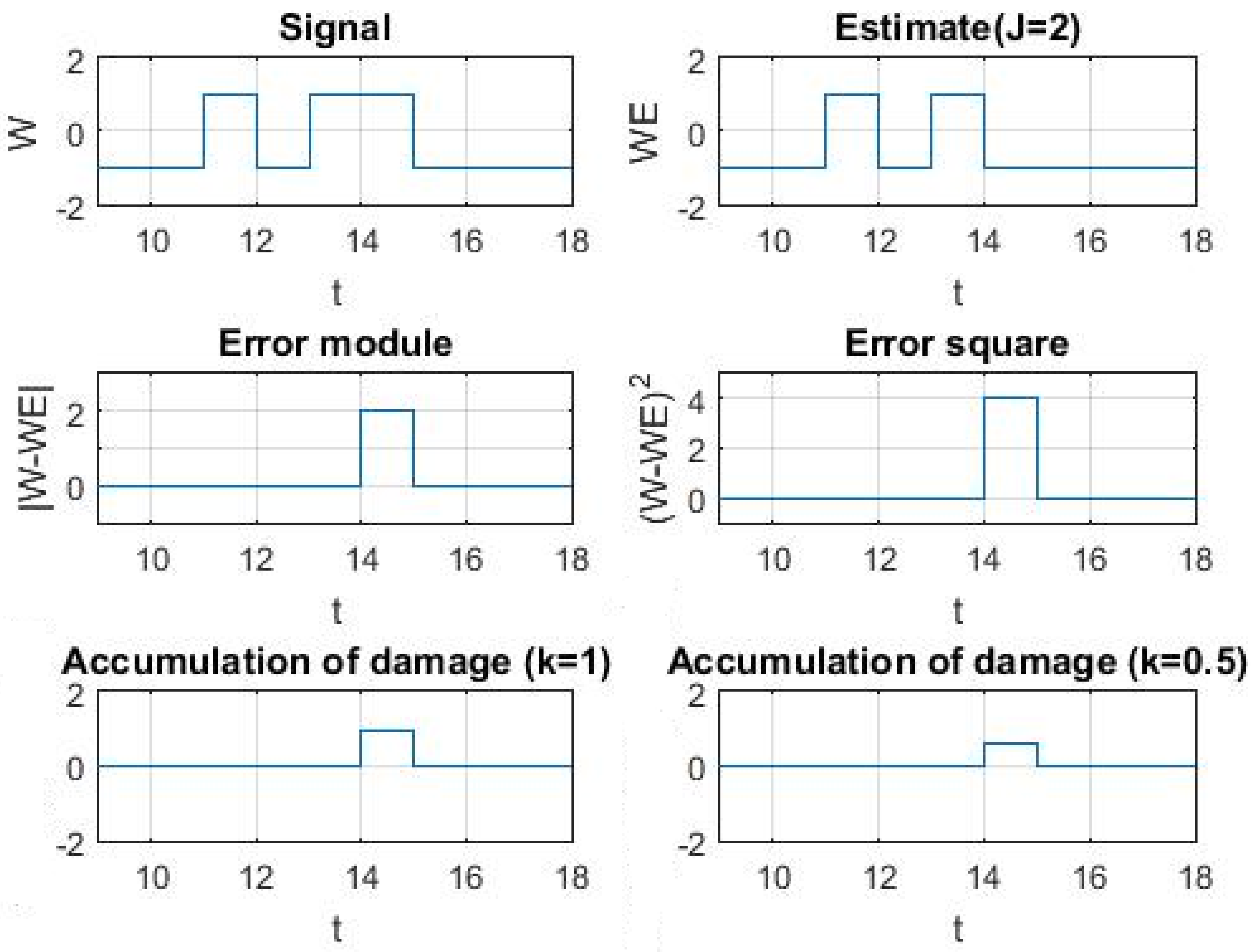
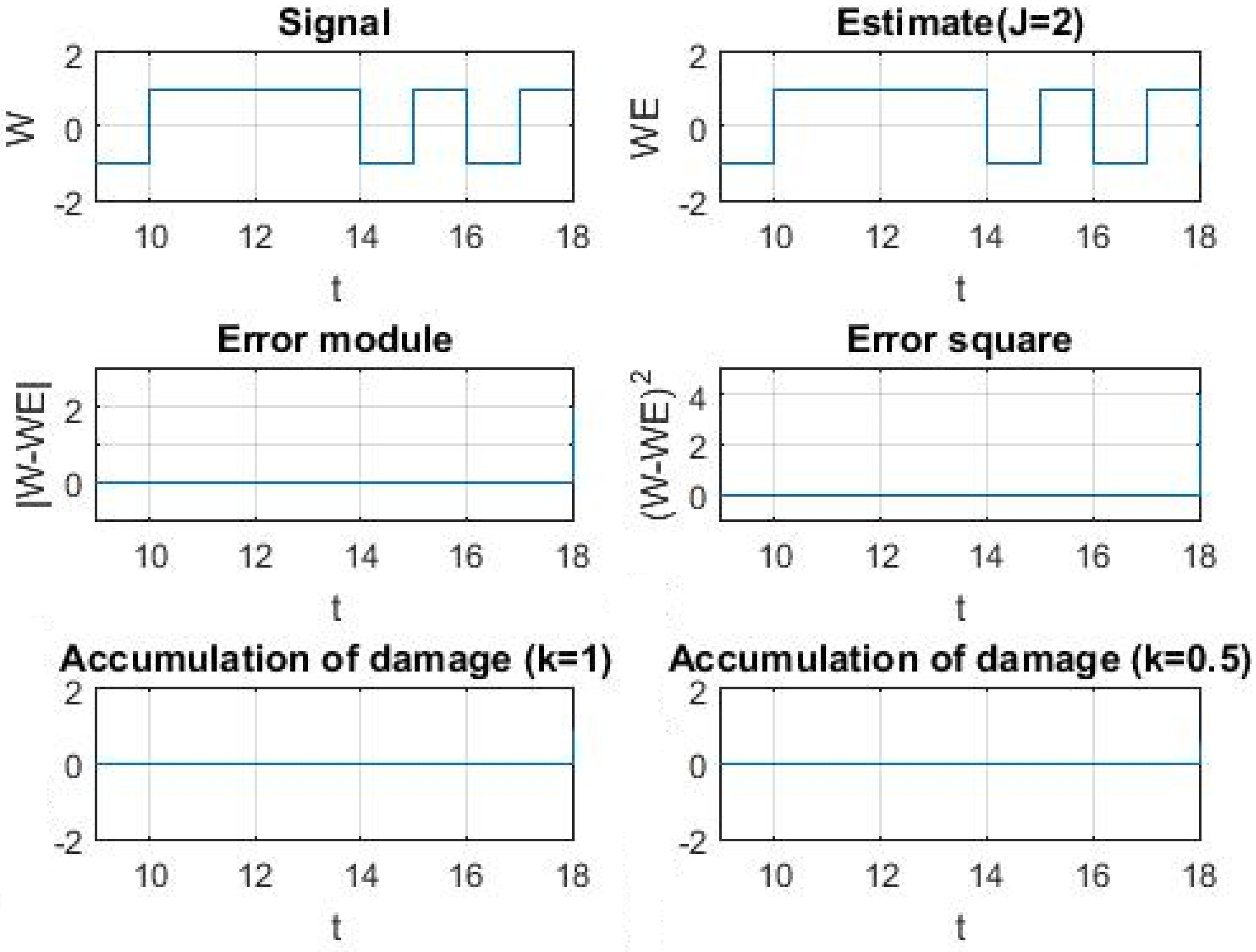
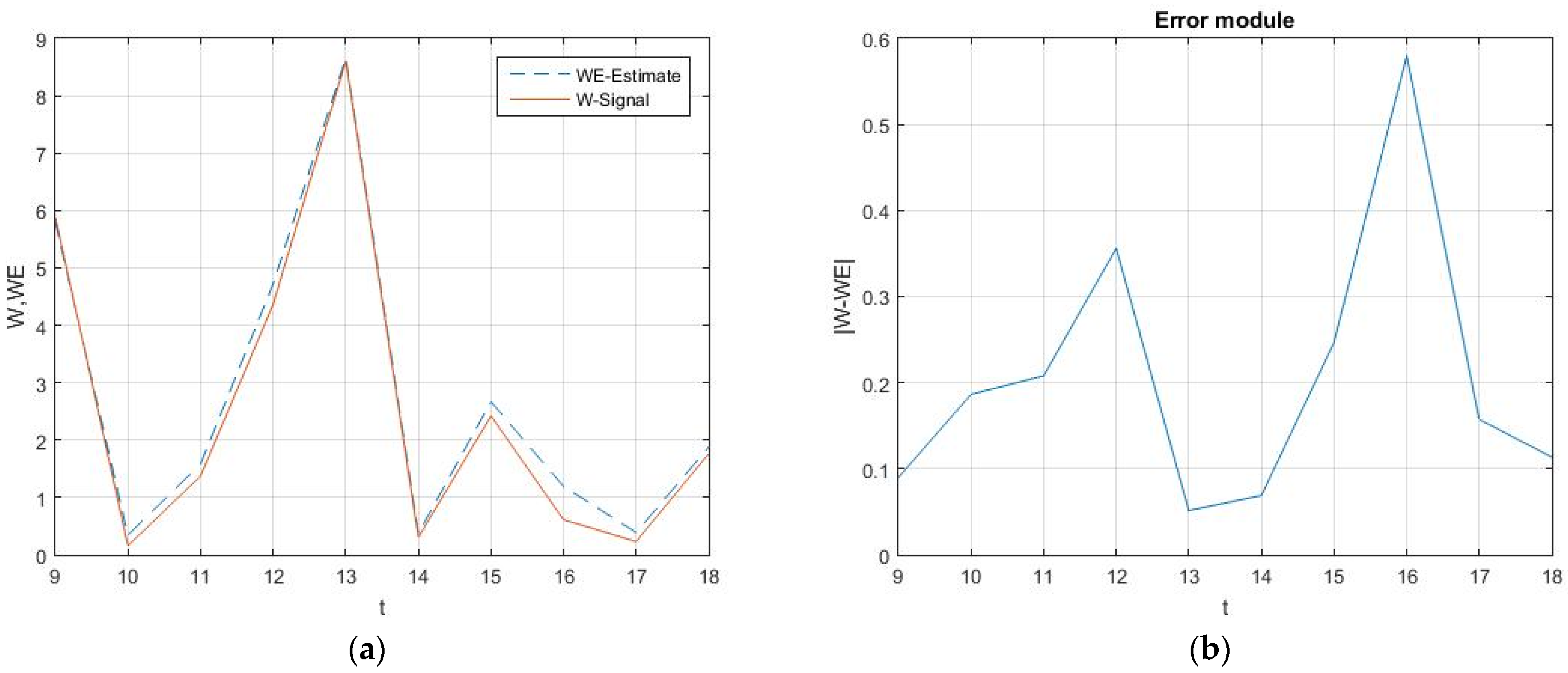
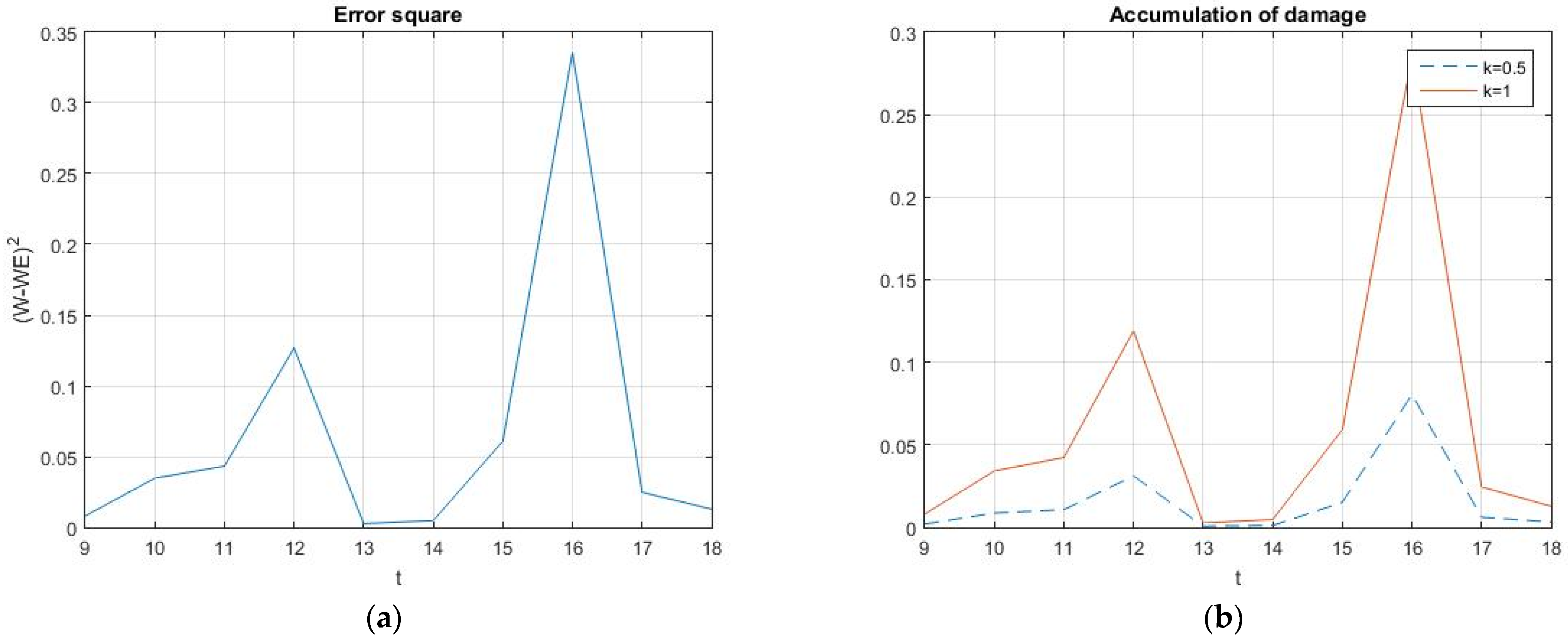
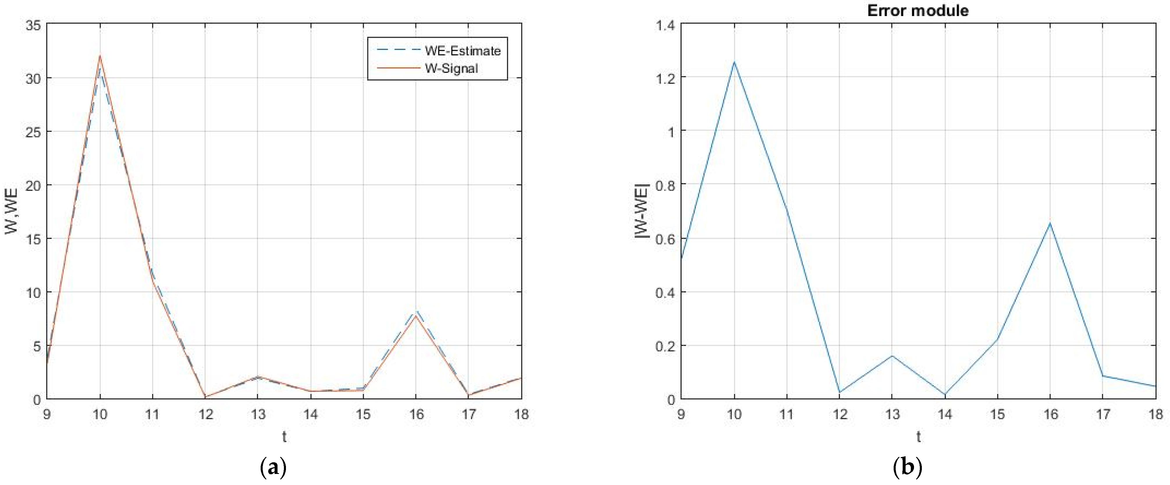
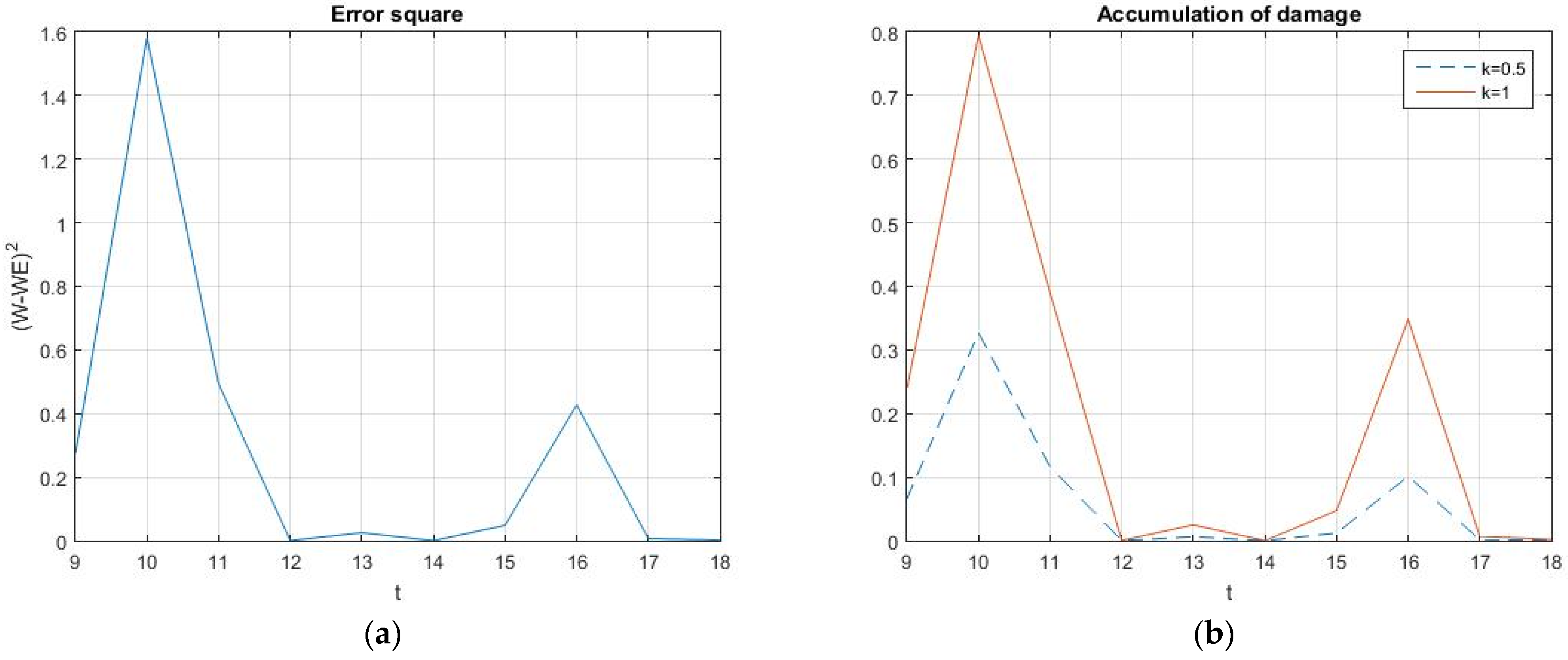
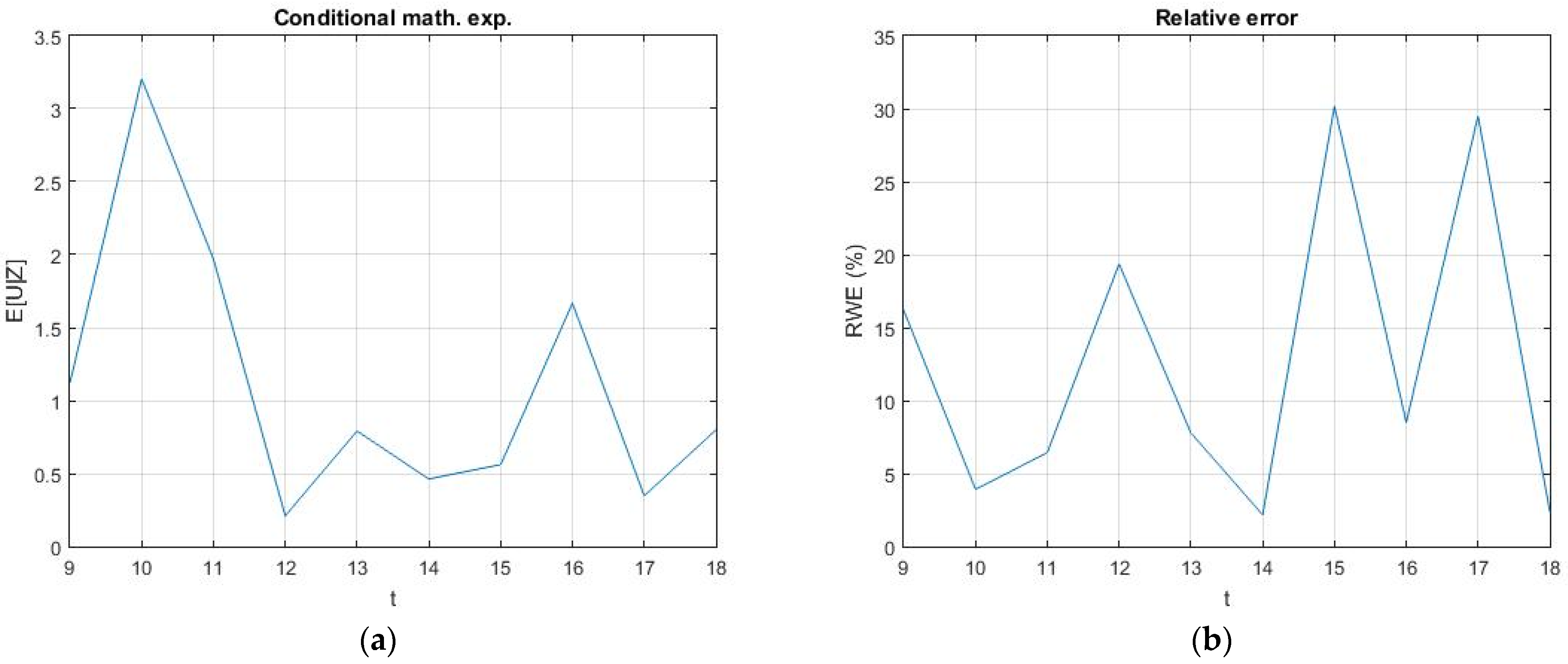
An important issue of the considered nonstationary stochastic systems is to obtain faster convergence speed. Structural functions and covariance functions of noises in our approaches demand one- and two-dimensional ${ℒ}^2$-spaces. We use Haar wavelets due to their simplicity and analytical expressions. It is known that wavelet expansions based on Haar wavelets have poor convergence compared to wavelet expansions based on, for example, Daubechies wavelets. We suggest two ways for the improvement of convergence speed: (i) increase the maximal level of revolution of fix wavelet bases; (ii) choice of fixed type of carrier. Computer experiments in Examples 1–3 confirm good engineering accuracy even for resolution two levels and eight members of canonical expansions.

For the NLOStSs described, stochastic differences and differential equations corresponding to algorithms are given in [2,3,4]. Applications:

–

Approximate linear and equivalent linearized model building for observable nonstationary and nonlinear stochastic systems;

–

Bayes’ criterion optimization and the calibration of parameters in complex quality measurement and control systems;

–

Estimation of potential efficiency of nonstationary nonlinear stochastic systems;

–

Directions of future generalizations and implementations;

–

New models of scalar- and vector-observable stochastic systems (nonlinear, with additive and parametric noises, etc.);

–

New classes of Bayes’ criterion (integral, functional, mixed);

–

Implementation of wavelet-integral canonical expansions for hereditary stochastic systems.

This research was carried out using the infrastructure of the Shared Research Facilities “High Performance Computing and Big Data” (CKP “Informatics”) of FRC CSC RAS (Moscow, Russia).