Abstract
Higher-order dynamic mode decomposition (HODMD) has proved to be an efficient tool for the analysis and prediction of complex dynamical systems described by data-driven models. In the present paper, we propose a realization of HODMD that is based on the low-rank tensor decomposition of potentially high-dimensional datasets. It is used to compute the HODMD modes and eigenvalues to effectively reduce the computational complexity of the problem. The proposed extension also provides a more efficient realization of the ordinary dynamic mode decomposition with the use of the tensor-train decomposition. The high efficiency of the tensor-train-based HODMD (TT-HODMD) is illustrated by a few examples, including forecasting the load of a power system, which provides comparisons between TT-HODMD and HODMD with respect to the computing time and accuracy. The developed algorithm can be effectively used for the prediction of high-dimensional dynamical systems.
Keywords:
higher-order dynamic mode decomposition; tensor-train decomposition; dynamic systems; data-driven model; power systems MSC:
15A69; 37M10; 37M99; 37N93
1. Introduction
Dynamical systems appear in many applications in physics. The description of a complex dynamical system can be unfeasible because the physical model is too complicated. In this way, data-driven models based on the dynamic mode decomposition (DMD) [1] can be effectively used. Such models are entirely based on measured data (snapshots) obtained over time. With the use of DMD, key dynamic modes can be identified that drastically reduce the computational complexity of the problem and lead to a reduced-order model.
Higher-order dynamic mode decomposition (HODMD), which was first introduced by Le Clainche and Vega [2], is an extension of the dynamic mode decomposition. HODMD extends the application of the standard DMD to the data with the spatial complexity less than the spectral complexity. This occurs when the spatial dimension is less than the number of dynamical modes, for example, in the Lorenz system [3]. The efficiency of HODMD has been confirmed numerous times in the literature for different applications such as the study of flow dynamics from numerical and experimental data [4,5,6,7], filtering experimental noise from a limited number of snapshots [8,9] and prediction of load for power systems [10].
However, it is problematic to use HODMD for high-dimensional systems because of the curse of dimensionality when the computational complexity growths exponentially with the increase of dimension. As a result, only quite a limited amount of data can be analyzed. Some tensor formats have been proposed to mitigate this problem such as the canonical tensor format, the Tucker format, or the tensor-train format (TT-format). While the canonical format is structurally the simplest, it is well known that it is numerically unstable, as the approximation with a fixed canonical rank in the Frobenius norm can be ill-posed [11]. At the same time, computing the canonical rank is an NP-hard problem (non-deterministic polynomial–time problem) [12]. Furthermore, despite the Tucker format being numerically stable, it suffers from the so-called curse of dimensionality, as the size of the core tensor grows exponentially with the increase of the number of dimensions [13]. To overcome this problem, the tensor-train decomposition (TTD) [12] can be used. TTD can be interpreted as a multi-dimensional generalization of the singular value decomposition (SVD). As a result, TTD incorporates the advantages from both the canonical formats and Tucker formats and can be efficiently applied to high-dimensional problems. A tensor-train-based DMD has recently been proposed in [14] where it is demonstrated that the realization of DMD in the TT-format significantly increases the efficiency of the entire algorithm.
The main objective of this paper is to make the use of HODMD more efficient and feasible for high-dimensional dynamical systems. For this purpose, we realize HODMD in TT-format for the first time. The proposed algorithm can be applied, in particular, to DMD that leads to a modified TT-DMD algorithm.
This paper is organized as follows. Section 2 briefly describes the standard HODMD. Then, Section 2.2 introduces the TT-format first. Then, it is extended to HODMD with the TT-HODMD algorithm. Effectively, the proposed algorithm can be applied to DMD, which leads to an alternative realization of TT-DMD. In Section 3, numerical results for comparison between TT-HODMD and HODMD are presented. They are first applied to an analytical example for validation purposes. Then, a practical application is considered. In this example, HODMD is used for a long-term prediction of the electrical power load in a power grid. It is demonstrated that the developed technique is capable of tremendously reducing the computing time that makes the algorithm potentially valuable for a real-time control. Finally, the proposed realization of TT-DMD is compared against the algorithm presented in [14] with respect to the computing time. Finally, the conclusion is provided in Section 4.
2. Methods
In this section, we first introduce HODMD. Then, we use SVD to reduce data and effectively calculate HODMD modes and eigenvalues. Finally, we rewrite the algorithm with the use of the low-rank decomposition of potentially high-dimensional data.
The algorithm of HODMD presented in this section is explained in more detail in [2]. In contrast to [2], we introduce it as a temporary convolution.
2.1. High-Order Dynamic Mode Decomposition
Consider a dataset of K equispaced snapshots collected at time instant (). For further consideration, we suppose that in the general case, snapshots represent tensors of dimension m: , . As such, vector is obtained via unfolding tensor .
The key DMD assumption is that there is a linear operator which allows us to predict each snapshot from the previous one. As noted by Mezić [15], this operator can be interpreted as a finite-dimensional approximation of the Koopman operator. As a rule, the DMD assumption is only valid to some extend, and to approximate the DMD operator, a large set of data is needed.
In contrast to DMD, HODMD is based on more series of snapshots in such a way that each snapshot is supposed to be related with d previous consequent snapshots via some linear operators:
where . It is worth noting that such an extension is especially important when the temporal complexity exceeds the spatial complexity.
It is clear that in case , we obtain the standard DMD approach. It is interesting to note that Equation (1) represents a discrete convolution over time. It provides a relationship between the HODMD and Mori–Zwanzig formalism [16]. Thus, the first term represents the Markovian term and approximates the Koopman operator. At the same time, the sum in Equation (1) can be interpreted as the memory term with a kernel having a bounded support. The bounded support is justified since, as noted in [16], the kernel vanishes for large enough times. In the framework of the Koopman analysis, the kernel contains the contribution of unresolved observables over time. The omitted noise term on the right-hand side represents the contribution of unresolved dynamics. The Koopman operator is adjoint to the Perron–Frobenius operator [17] used for the analysis of dynamical systems. Thus, approximation (1) of the Koopman operator can be considered as an alternative approach to the approximation of the Perron–Frobenius operator [18].
Next, we split all snapshots onto overlapping matrices with elements each:
where . Then, we can rewrite Equation (1) as follows:
To reduce the dimension of the data considered, we apply the singular value decomposition (SVD) to the snapshot matrix , written in the SVD format as
where
The diagonal of matrix contains the singular values , . Here, we presume that matrices and are unitary and all singular values are numerated according to their diminishing: . In addition, suppose that starting from some element , the singular values can be truncated: , where is small enough. Thus, we introduce the threshold parameter to determine the error of approximation in the Frobenius norm in the case of truncation.
The orthonormal columns of unitary matrix and unitary matrix are the spatial and temporal SVD-modes, respectively. The rows of the matrix are proportional to the SVD temporal modes and can be seen as rescaled temporal modes. Equation (3) implies that the snapshots can be projected onto the subspace of SVD spatial modes which can have a much lower dimension depending on N. In that space, we then consider snapshots from .
Now, we can formulate the DMD-d algorithm for the reduced snapshot matrices as follows:
where , , and for .
Recurrently, from Equation (5), we obtain the following relationship
between and , where the reduced modified snapshot matrix is given by
In turn
Here, matrices and are supposed to be known from measurements.
It is well known that the solution to the overdetermined system (6) in the Frobenius norm is obtained via the pseudo-inverse matrix of :
where
Then, its eigenvectors, called HODMD modes and eigenvalues , can be immediately calculated. These eigenvalues coincide with the eigenvalues of the transition operator for the original snapshots:
Indeed, then
and
where , is a unit matrix. Hence
Thus, if and are the eigenvalue and eigenvector of matrix , respectively, then is an eigenvalue of matrix and the appropriate eigenvector is given by
More precisely, this is a DMD mode projected onto the space of snapshots by the previous time step while the exact mode can be calculated as [19]
Then, the snapshots can be expanded via DMD modes:
where , is a growth mode, is a frequency, and M is the number of retained DMD modes that represents the spectral complexity.
The amplitudes can be determined from fitting the snapshots in the Frobenius norm. In this way, it is more efficient to consider the reduced snapshots [2].
Then, we arrive at equation
where
Equation (17) can be immediately solved via the pseudo-inverse matrix to calculated via SVD.
2.2. Proposed Algorithm
In this subsection, we first describe the tensor-train format (TT-format) and then show how HODMD can be realized with TTD. The aim is to make the application of HODMD more efficient to analyze dynamical systems of high dimension.
2.2.1. TT-Format
Over the last years, different tensor formats such as the canonical format, the Tucker format, and the TT-format have been developed, see e.g., [20,21,22,23,24]. The TT-format is not affected by the curse of dimensionality; in addition, it provides a very efficient way to use basic linear algebra and rounding operations when the data are formatted [12].
The TTD is introduced in detail in [12]. Here, we repeat the main algorithm. Consider a data array presented as tensor . First, we can split the dimension into two parts: and . Then, we are able to reshape into a matrix based on and , which is marked as . This process is called the matricization. After the matricization, it is possible to compute SVD for this reshaped matrix as follows:
where and , . Here, is formally introduced to retain a uniform approach.
In the second approximate equality, we presume that all singular values exceed some threshold and their number is equal to . Thus, determines the tensor rank. Next, matrix is reshaped into matrix
for which threshold is introduced that determines rank of the SVD decomposition for . Thus, and . This procedure is repeated until the final index .
In this way, the first TT-core is obtained by reshaping matrix into a tensor with dimension . In turn, the second TT-core is determined by reshaping matrix into a tensor with dimension . Finally, the TT-decomposition of can be presented in the following form
Thus, the original tensor can be approximated and reconstructed via a series of multilinear products between the cores. Formally, each core represents a tensor with the order of three. At the same time, the order of the first and last cores is actually reduced to two.
Figure 1 depicts the TT-decomposition of a 4-dimensional tensor (inspired by [25]). A tensor of size can be decomposed into four parts. Four rows in the figure represent four types of expressions: (from top to bottom) regular, kernel-linked, fibres, and slices. All four types of expressions represent a schematic description of the TT-decomposition. It looks like a train with carriages and links between them, and that justifies the name of the algorithm [12].
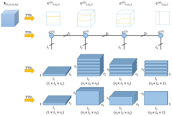
Figure 1.
TT-decomposition of 4-dimensional tensor .
2.2.2. Tensor-Train-Based HODMD
In this section, we introduce the TT-based HODMD algorithm. It is novel not only in application to HODMD but also if applied to DMD when .
Next, we fold vectors as tensors .
Then, we decompose each tensor with TT-SVD:
We presume tensor :
is left–orthonormal: . Any tensor train can be orthogonalized [12]. Therefore, our assumption does not violate the generality.
Thus,
where
is a unitary matrix: .
Multiplying Equation (1) by , we arrive at equation:
where .
Thus, we effectively reduce the analysis to the evolution of the temporary modes . As soon as the temporary modes are obtained, the full vectors of snapshots can be immediately restored via Equation (23):
Next, we can apply the HODMD analysis described in Section 2 immediately.
3. Results and Discussion
Accurate power load forecasting has important practical value and significance for ensuring the economic and safe operation of the power service sector [26]. In the energy interconnection system, with the development of communication technology and the application of measurement equipment, relevant departments obtain large amounts of information data, which can be exploited for improving the performance of load forecasting models.
For the power sector, to better formulate grid dispatch plans and optimize the daily power generation plan of conventional power sources, short-term load forecasting (STLF) is often used to obtain electrical loads for 1 to 3 days (1 to 72 h). According to the technical characteristics of STLF, it can be roughly divided into statistical models, neural network models and combined forecasting models. The forecasting model should be reasonably selected according to the specific forecasting environment and the characteristics of the input data [27,28]. Among them, HODMD-based STLF techniques have gradually attracted attention due to their good properties, which do not depend on any given dynamic system expression [10]. At the same time, the data obtained in the power system have obvious big data “4V” characteristics [29] (i.e., high Veracity, high Variety, high Velocity and high Value), and it is attractive to use TT-HODMD to achieve more efficient short-term forecasting.
In the case of this section, we realize the load forecasting of the power system by generating a short-term forecasting model based on HODMD and TT-HODMD. First, we verify the proposed TT-HODMD algorithm. Subsequently, we apply both HODMD and TT-HODMD for short-term forecasting through a simple power system example. Finally, we present the analysis of the obtained results and comparison of alternative algorithms.
In the numerical experiments, the codes are developed in Spyder (Python 3.7) and the calculations are implemented on a MacOS machine with Intel Core i5 CPU (2.4 GHz), 8 GB RAM and 4 cores.
3.1. Validation of TT-HODMD
We use a test dataset to validate the TT-HODMD code developed. This dataset is obtained from function f which is created by the following function:
The temporal part of the test function is taken from a test case presented in [2]. In this test case, the spatial complexity is always supposed to be less than the spectral complexity such that DMD is not immediately applicable.
Next, we introduce uniform meshing for x with 400 nodes and consider 1000 equispaced snapshots. The function is shown in Figure 2a, where the horizontal coordinate is x, the vertical coordinate corresponds to t and the shade of color represents the value of f. In Figure 2b, the horizontal coordinate corresponds to the snapshots whilst the vertical coordinate is . For the test case, the data generated via the function are formally folded in a array.
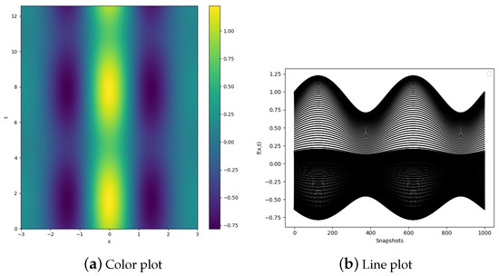
Figure 2.
Function .
As an example, we compare the results against all snapshots at the row: . The intercepted part is presented by the solid line in Figure 3.
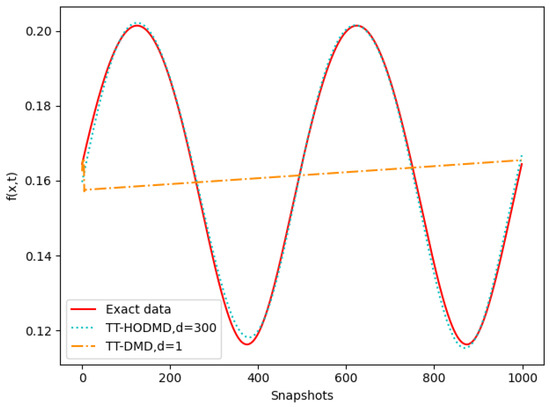
Figure 3.
Comparison of TT-DMD and TT-HODMD .
Next, we assume , which brings us to a modified dataset, further called , with the size of (see Equation (10) for details).
From Section 2, is considered as a threshold parameter for HODMD and TT-HODMD. The thresholds are supposed to be equal to .
Figure 3 shows the comparison of reconstructions with TT-HODMD and TT-HODMD . It is clear that the algorithm with fails to reconstruct the dataset. In this case, TT-DMD does not reproduce the number of modes sufficient for reconstruction. By contrast, the TT-HODMD with is capable of reconstructing the function f. A relatively high value of d provides a high degree of delay-embedding without excessive loss of influence of the later snapshots.
Next, with , we select the row of the dataset: . Figure 4 demonstrates the sensitivity of the reconstruction to the threshold . As expected with the decrease of , TT-HODMD provides the reconstruction closer to the result with HODMD thanks to the decrease of TT thresholds .
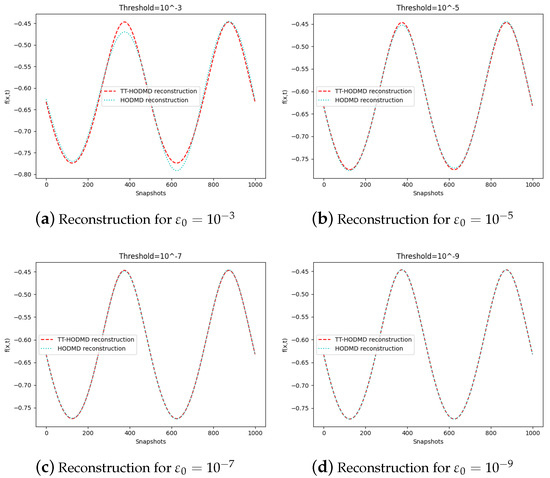
Figure 4.
Reconstruction by TT-HODMD and HODMD with different thresholds.
The results for prediction obtained for different d for are presented in Figure 5.
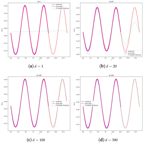
Figure 5.
Prediction with different d.
As a quantitative measure, we use RMSE (root mean square error) to estimate the deviation between the predicted and real values:
where is the vector of predicted values and represents the real values. The comparison of RMSE with different d values is shown as Table 1. As can be seen, the prediction with is very close to the exact result. In turn, the standard DMD with fails. As noted in [2], an optimal d essentially depends on K.

Table 1.
RMSE of different d.
3.2. Realization of STLF in Power System Based on TT-HODMD
A real STLF simulation analysis in a power system is presented in this section. The data are taken from the UK National Grid Electricity System Operator [30]. In this test case, we select three years of historic demand data for simulation. We choose 12 months of data per year, 20 days of data per month, 24 h of data per day, and then the data are measured every 15 minutes (resulting in 96 data per day). In this way, we obtain three-dimensional data of , where the last figure represents the number of units per month. On the basis of three-year load data, we predict the power load for the next six months starting from January 2020. In this way, we compare TT-HODMD and HODMD with respect to the accuracy, robustness and computing time.
The tensor-based data model is more useful for analyzing and processing data than the traditional time series. The differences between the tensor-based data and traditional time-series-based data are presented in Table 2 in terms of data structure, data meaning and data processing, respectively.
Table 2.
The difference between tensor-based data and time-series-based data.
As discussed in Section 2.2.2, we only consider the temporary modes . The results obtained by TT-HODMD with are shown in Figure 6. As can be seen, TT-HODMD with , which is around 20% of the number of snapshots, provides a much better reconstruction and prediction.
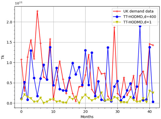
Figure 6.
Comparison of TT-HODMD prediction with and against real UK demand data.
It is worth noting that HODMD allows us to effectively analyze the stability of a power system. Figure 7 demonstrates the DMD eigenvalues from Equation (16) obtained with . These eigenvalues correspond to the Koopman transition operator [31] and determine the stability of the power system in study. As can be seen from Figure 7, the considered power system is stable since there are no modes with the eigenvalues outside the unit circle. The modes with the eigenvalues situated inside the unit circle vanish over time, whilst the others retain stable.
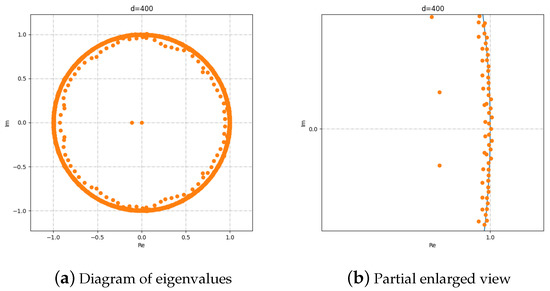
Figure 7.
Eigenvalues with .
The key comparison of TT-HODMD and HODMD is related to the runtime. It is shown in Figure 8 for different thresholds . As can be seen, the threshold has much greater impact on HODMD, whilst it is very well mitigated with TT-HODMD. Thus, with the increase of the accuracy of prediction, TT-HODMD has a tremendous advantage.
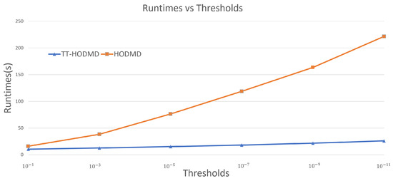
Figure 8.
Runtime of HODMD and TT-HODMD applied to given STLF system based on for different values of .
Finally, in Figure 9, we compare the proposed algorithm for TT-DMD against the approach from [14] for different thresholds. A principal difference between the two approaches is that in our algorithm, we effectively consider only temporary modes that significantly improve the efficiency. It is clear that this effect becomes more significant with the increase of the number of modes. In turn, the number of modes involved is determined by the threshold. As a result, with the decrease of the threshold, the proposed approach essentially overcomes the algorithm from [14].
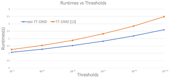
Figure 9.
Comparison of the runtime of TT-DMD [14] algorithm and new TT-DMD algorithm applied to given STLF system for different values of thresholds.
4. Conclusions
In this paper, a new approach to the tensor-train realization of dynamic mode decomposition has been proposed. It is effectively reduced to the computation of temporary modes in an orthogonal basis. The algorithm has been implemented to realize the High-Order DMD in the TT-format for the first time and applied to the forecasting of load in a power system. It is demonstrated that in comparison to DMD, HODMD has a significant advantage in its capability of reconstructing and predicting load data. In contrast to the original HODMD, the developed TT-HODMD algorithm has very little sensitivity to the value of the threshold with respect to the runtime. With the increase of the accuracy of prediction, TT-HODMD operates much faster than HODMD. In addition, it is shown that the proposed approach to TT-DMD is essentially faster than the existing algorithm already known in the literature. The developed algorithm can be effectively applied to real-life problems such as the prediction of the load in a power system.
Author Contributions
K.L. wrote a code, carried out numerical experiments, and prepared all figures. S.U. developed the algorithm and analyzed the results. All authors have read and agreed to the published version of the manuscript.
Funding
This research is funded by Engineering and Physical Sciences Research Council, EP/V038249/1.
Institutional Review Board Statement
Not applicable.
Informed Consent Statement
Not applicable.
Data Availability Statement
No new data were generated or analysed during this study.
Acknowledgments
The authors are grateful to the unknown referees for helpful remarks which improved the quality of the paper.
Conflicts of Interest
The authors declare no conflict of interest.
Abbreviations
The following abbreviations are used in this manuscript:
| DMD | Dynamic mode decomposition |
| HODMD | Higher-order dynamic mode decomposition |
| TT-format | Tensor-train format |
| TTD | Tensor-train decomposition |
| SVD | Singular value decomposition |
| TT-HODMD | Tensor train-based higher order dynamic mode decomposition |
| STLF | Short-term load forecasting |
| TT-DMD | Tensor train-based dynamic mode decomposition |
References
- Schmid, P.J. Dynamic mode decomposition of numerical and experimental data. J. Fluid Mech. 2010, 656, 5–28. [Google Scholar] [CrossRef]
- Le Clainche, S.; Vega, J.M. Higher order dynamic mode decomposition. SIAM J. Appl. Dyn. Syst. 2017, 16, 882–925. [Google Scholar] [CrossRef]
- Lorenz, E.N. Deterministic nonperiodic flow. J. Atmos. Sci. 1963, 20, 130–141. [Google Scholar] [CrossRef]
- Mengmeng, W.U.; Zhonghua, H.A.N.; Han, N.I.E.; Wenping, S.O.N.G.; Le Clainche, S.; Ferrer, E. A transition prediction method for flow over airfoils based on high-order dynamic mode decomposition. Chin. J. Aeronaut. 2019, 32, 2408–2421. [Google Scholar]
- Le Clainche, S.; Han, Z.H.; Ferrer, E. An alternative method to study cross-flow instabilities based on high order dynamic mode decomposition. Phys. Fluids 2019, 31, 094101. [Google Scholar] [CrossRef]
- Le Clainche, S.; Vega, J.M. Higher order dynamic mode decomposition to identify and extrapolate flow patterns. Phys. Fluids 2017, 29, 084102. [Google Scholar] [CrossRef]
- Kou, J.; Le Clainche, S.; Zhang, W. A reduced-order model for compressible flows with buffeting condition using higher order dynamic mode decomposition with a mode selection criterion. Phys. Fluids 2018, 30, 016103. [Google Scholar] [CrossRef]
- Le Clainche, S.; Vega, J.M.; Soria, J. Higher order dynamic mode decomposition of noisy experimental data: The flow structure of a zero-net-mass-flux jet. Exp. Therm. Fluid Sci. 2017, 88, 336–353. [Google Scholar] [CrossRef]
- Le Clainche, S.; Sastre, F.; Vega, J.M.; Velazquez, A. Higher order dynamic mode decomposition applied to post-process a limited amount of noisy PIV data. In Proceedings of the 47th AIAA Fluid Dynamics Conference, Denver, CO, USA, 5–9 June 2017. [Google Scholar]
- Jones, C.; Utyuzhnikov, S. Application of higher order dynamic mode decomposition to modal analysis and prediction of power systems with renewable sources of energy. Int. J. Electr. Power Energy Syst. 2022, 138, 107925. [Google Scholar] [CrossRef]
- Kressner, D.; Tobler, C. Low-rank tensor Krylov subspace methods for parametrized linear systems. SIAM J. Matrix Anal. Appl. 2011, 32, 1288–1316. [Google Scholar] [CrossRef]
- Oseledets, I.V. Tensor-train decomposition. SIAM J. Sci. Comput. 2011, 33, 2295–2317. [Google Scholar] [CrossRef]
- Holtz, S.; Rohwedder, T.; Schneider, R. The alternating linear scheme for tensor optimization in the tensor train format. Siam J. Sci. Comput. 2012, 34, A683–A713. [Google Scholar] [CrossRef]
- Klus, S.; Gelß, P.; Peitz, S.; Schütte, C. Tensor-based dynamic mode decomposition. Nonlinearity 2018, 31, 3359. [Google Scholar] [CrossRef]
- Mezić, I. Analysis of fluid flows via spectral properties of the Koopman operator. Annu. Rev. Fluid Mech. 2013, 45, 357–378. [Google Scholar] [CrossRef]
- Lin, Y.T.; Tian, Y.; Livescu, D.; Anghel, M. Data-Driven Learning for the Mori–Zwanzig Formalism: A Generalization of the Koopman Learning Framework. SIAM J. Appl. Dyn. Syst. 2021, 20, 2558–2601. [Google Scholar] [CrossRef]
- Ding, J.; Du, Q.; Li, T.Y. High Order Approximation of the Frobenius-Perron Operator. Appl. Math. Comput. 1993, 53, 151–171. [Google Scholar] [CrossRef]
- Klus, S.; Koltai, P.; Schtte, C. On the numerical approximation of the Perron-Frobenius and Koopman operator. J. Comput. Dyn. 2016, 3, 51–79. [Google Scholar]
- Tu, J.H. Dynamic Mode Decomposition: Theory and Applications. Ph.D. Thesis, Princeton University, Princeton, NJ, USA, 2013. [Google Scholar]
- Beylkin, G.; Mohlenkamp, M.J. Numerical operator calculus in higher dimensions. Proc. Natl Acad. Sci. USA 2002, 99, 10246–10251. [Google Scholar] [CrossRef]
- Grasedyck, L.; Kressner, D.; Tobler, C. A literature survey of low-rank tensor approximation techniques. GAMM-Mitt. 2013, 36, 53–78. [Google Scholar] [CrossRef]
- Hackbusch, W. Tensor Spaces and Numerical Tensor Calculus; Springer: Berlin, Germany, 2012; Volume 42. [Google Scholar]
- Hackbusch, W. Numerical tensor calculus. Acta Numer. 2014, 23, 651–742. [Google Scholar] [CrossRef]
- Yang, J.-H.; Zhao, X.-L.; Ji, T.-Y.; Ma, T.-H.; Huang, T.-Z. Low-rank tensor train for tensor robust principal component analysis. Appl. Math. Comput. 2020, 367, 124783. [Google Scholar] [CrossRef]
- Cichocki, A. Era of big data processing: A new approach via tensor networks and tensor decompositions. In Proceedings of the Conference: International Workshop on Smart Info-Media Systems in Asia, Nagoya, Japan, 30 September–2 October 2013. [Google Scholar]
- Garulli, A.; Paoletti, S.; Vicino, A. Models and techniques for electric load forecasting in the presence of demand response. IEEE Trans. Control Syst. Technol. 2014, 23, 1087–1097. [Google Scholar] [CrossRef]
- Wang, Z.; Zhao, B.; Ji, W.; Gao, X.; Li, X. Short-term load forecasting method based on GRU-NN model. Autom. Electr. Power Syst. 2019, 43, 53–62. [Google Scholar]
- Hong, T.; Pinson, P.; Fan, S. Global energy forecasting competition 2012. Int. J. Forecast. 2014, 30, 357–363. [Google Scholar] [CrossRef]
- Cichocki, A. Tensor networks for big data analytics and large-scale optimization problems. arXiv 2014, arXiv:1407.3124. [Google Scholar]
- Nationalgrid.com. Demand Forecasting|National Grid Gas. 2022. Available online: https://www.nationalgrid.com/gas-transmission/about-us/system-operator-incentives/demand-forecasting (accessed on 13 July 2022).
- Hemati, M.S.; Williams, M.O.; Rowley, C.W. Dynamic mode decomposition for large and streaming datasets. Phys. Fluids 2014, 26, 111701. [Google Scholar] [CrossRef]


Disclaimer/Publisher’s Note: The statements, opinions and data contained in all publications are solely those of the individual author(s) and contributor(s) and not of MDPI and/or the editor(s). MDPI and/or the editor(s) disclaim responsibility for any injury to people or property resulting from any ideas, methods, instructions or products referred to in the content. |
© 2023 by the authors. Licensee MDPI, Basel, Switzerland. This article is an open access article distributed under the terms and conditions of the Creative Commons Attribution (CC BY) license (https://creativecommons.org/licenses/by/4.0/).