Abstract
We present a study on modelling American Sign Language (ASL) with encoder-only transformers and human pose estimation keypoint data. Using an enhanced version of the publicly available Word-level ASL (WLASL) dataset, and a novel normalisation technique based on signer body size, we show the impact model architecture has on accurately classifying sets of 10, 50, 100, and 300 isolated, dynamic signs using two-dimensional keypoint coordinates only. We demonstrate the importance of running and reporting results from repeated experiments to describe and evaluate model performance. We include descriptions of the algorithms used to normalise the data and generate the train, validation, and test data splits. We report top-1, top-5, and top-10 accuracy results, evaluated with two separate model checkpoint metrics based on validation accuracy and loss. We find models with fewer than 100k learnable parameters can achieve high accuracy on reduced vocabulary datasets, paving the way for lightweight consumer hardware to perform tasks that are traditionally resource-intensive, requiring expensive, high-end equipment. We achieve top-1, top-5, and top-10 accuracies of , , and , respectively, on a vocabulary size of 10 signs; , , and on 50 signs; , , and on 100 signs; and , , and on 300 signs, thereby setting a new benchmark for this task.
Keywords:
sign language recognition; human pose estimation; classification; computer vision; deep learning; machine learning; supervised learning MSC:
68T10; 68T45; 68T50
1. Introduction
Research in computational modelling of sign language has seen increasing attention since the 1980s, often under the guise of gesture recognition for human–computer interaction (HCI), for which sign language proves to be a convenient target dataset. The majority of the static hand configurations of the fingerspelled American Sign Language (ASL) alphabet was used in early gesture recognition research [1,2]. Motivated by the work of sign language linguistics pioneer Stokoe [3], Tamura and Kawasaki [4] began modelling sign language at the chereme level—the sub-unit equivalent of phonemes in spoken language [5]—which provided a mechanism for recognising manual signs that was rooted in linguistics. Modelling sign sub-units continued to form the basis for some sign language research see e.g., [6,7,8,9,10,11,12,13,14,15,16,17], justifying the linguistics-oriented approach.
In stark contrast, and in particular with the introduction of transformer neural networks [18] and their derivatives e.g., [19], explicitly modelling linguistic features of sign language can be forgone in favour of harnessing the power of deep learning to recognise patterns inherent in the data. This can greatly simplify model architecture, including reducing the number of learnable parameters and the need to heavily preprocess data. Moreover, the time and resources required to develop and deploy models can be significantly reduced, enabling the use of low-cost consumer and embedded hardware. This approach does have limitations, however, which becomes apparent when sign language recognition is not treated holistically, and instead as merely manual gesture recognition.
1.1. Sign Language
Sign language research has revealed a complexity and ability to communicate ideas that gives it parity with spoken language [20,21,22,23]. Along with a general increase in cultural and disability awareness, and focus on improving accessibility for Deaf communities, the research community started to embrace the multimodal aspects of sign language as well as the needs of the people it ostensibly intends to help [24]. At the very least, this amounts to a recognition that sign language goes beyond hand gestures [25,26], which has led to models increasingly utilising the whole signing space [27] and not just data derived from hands—although this practice does still continue largely via wearable technology e.g., [1,28,29,30,31,32,33,34,35,36], which has long been met with disdain by the Deaf community [37,38]. As with models that derive input data from video feeds that cover the signing space, those that incorporate data from human pose estimation keypoints can also inherently use the extra information available, though to what extent depends on the keypoints being used. This holistic view of the keypoints within the signing space is the approach we take in this study.
Dafnis et al. [39] emphasise the fact there is no one-to-one correspondence of ASL signs to English words. This is a well known relationship (or lack of) that exists between sign languages and the respective geographically located native spoken languages. Glosses are, by definition, a limited representation of a given sign, not a literal translation, and their use reinforces the misplaced idea that a universal one-to-one relationship exists. Efforts to codify glosses in linguistics research include annotations that provide more context than a single word representation, especially so that words with a common spelling, or similar signs that have subtle context-carrying variations, can be more easily differentiated [40,41,42,43,44].
1.2. Modelling
Many approaches to model aspects of sign language have been described in the literature. Hand-shape classification methods attempt to recognise specific configurations of hands [4,16,45,46,47,48], which can be considered the fundamental sign articulator—this has particular importance for recognising finger spelling [49]. Others focus on modelling non-manual aspects, which are essential context carriers, not least for discriminating between signs with similar appearance. For example, in German Sign Language (DSG), the signs for farbe and marmelade differ by accompanying mouth shape only [27]. The same is true in British Sign Language (BSL) for the signs for battery and uncle [50], and in ASL for late and not-yet [51] (which also includes a slight headshake in the latter sign). Instances where the mouth shapes are derived from the spoken language forms of the respective signs are known as speech-like mouthings [52]. To this end, research went further than classifying only hand shapes, to include mouth shapes [53,54], whole-face [55,56] and whole-body configurations [57,58], all in the context of sign language recognition and translation. The broader field of understanding sign language includes analyses of eyebrow position during signing to provide context and signer intent [59], further illustrating the importance of the holistic approach.
1.3. Datasets
One drawback of applying deep learning to challenging computational tasks is that such techniques are generally data hungry; for a model to generalise well to unseen data, it must be exposed to sufficient domain-representative examples during training, where it is common for datasets to contain millions of examples [60]. Computational sign language modelling research is hindered by a dearth of high-quality, large-sample, and freely available datasets containing diverse, Deaf—or otherwise, expert—signers. Efforts to help remedy this problem have increased over time, including for continuous sign language datasets. SIGNUM [61] is perhaps the first signer-independent corpus created specifically for computational sign language research, but has a limited vocabulary of 450 basic DSG signs. Nevertheless, it can likely be credited with helping kick-start the continuous sign language research movement e.g., [62,63,64,65]. The RWTH Phoenix dataset, which has seen at least three updates [66,67,68], is derived from public broadcasts of German weather reports, and has been a benchmark dataset for much research e.g., [63,65,69,70,71,72,73,74,75,76,77,78,79,80,81,82] despite the low video resolution and the limited domain (i.e., weather forecasts). With a vocabulary of approximately 3000 DSG signs, this in an improvement over SIGNUM, but is smaller still than the BSL Corpus dataset comprising approximately 5000 signs [83]. The current largest continuous sign language dataset is How2Sign [84], which despite containing a vocabulary on the order of 16,000 spoken language words, at the time of writing has no public release of accompanying glosses. In conjunction with transcription problems (e.g., character encoding errors, typing errors, signers’ names frequently being prepended to the transcription, to name a few), the lack of available glosses makes it more challenging to perform sign language translation using this dataset. For sign language recognition research, the largest dataset of so-called word-level signs—that is to say isolated, dynamic signs—is the Word-Level American Sign Language (WLASL) dataset [85], which has a vocabulary of 2000 signs by 119 signers across a total of 21,083 videos.
1.4. Our Approach
We present a way to model sign language using deep learning with a custom encoder-only transformer model, which is described in detail in Section 2.2. We analyse the architectural properties that can optimise the task. Specifically, we study modelling sign language using human keypoints extracted from sequences of isolated, dynamic signs, and perform sign recognition on a number of different sign classes, bench-marking the performance and model parameters at each stage. We test the scalability of this approach with number of sign classes by running multiple experiments on an enhanced version of WLASL.
The results provide an insight into encoder-only transformers for classifying sparse, noisy (and frequently incomplete), sequential data, and we show that simpler models can perform better than more complex models. Perhaps most surprisingly, we show that using an encoder-only transformer with a single layer and a single attention head is sufficient to perform this task well on reduced vocabulary datasets. Finally, we quantify the effect random number generation has on model performance, emphasising the importance of running many experiments when reporting results.
1.5. Related Work
Human pose estimation techniques for sign language recognition frequently employ multiple modalities beyond just keypoint coordinates. For context, we provide examples that take an appearance-based approach. Li et al. [85] apply transfer learning to fine tune the original Inflated 3D ConvNet (I3D) model [86] to output the required number of class probabilities. They achieve , , and for top-1, top-5, and top-10 accuracies, respectively, on WLASL with 100 sign classes, and , , on WLASL with 300 classes. In other work that uses motion and hand shapes to guide the pooling for a three-dimensional CNN on RGB video frames, Hosain et al. [87] achieve top-1, top-5, and top-10 accuracies on WLASL 100 of , , and , respectively, and , , on WLASL 300, using their Fusion-2 and Fusion-3 models.
To enable the best comparisons, we now focus on techniques that are not appearance-based, but instead are purely derived from human pose estimation keypoint data. We note, however, that because our study uses an enhanced version of WLASL, called WLASL-alt, as the basis of our experiments, comparisons are indicative of relative performance only. Nonetheless, there is substantial domain overlap making some comparison valid, i.e., the underlying keypoint values used are identical and it is only the class labels (glosses) and dataset splits that differ. Again, using the same top-1, top-5, and top-10 accuracy metrics, we provide performances from published work that uses keypoint data from WLASL only. Using a pose-based gated recurrent unit (Pose-GRU) to model the temporal motion of signs, Li et al. [85] achieve , , and on WLASL 100, and , , and on WLASL 300. They go on to apply a temporal graph convolutional network (Pose-TGCN) that achieves , , and on WLASL 100, and , , and on WLASL 300. Also using a graph convolutional network (GCN) approach, Tunga et al. [88] implemented a BERT-like network [19] to capture temporal interdependencies between frames in a given sequence, and report accuracies of , , and on WLASL 100, and , , and on WLASL 300. Bohacek and Hruz [89] report top-1 accuracies on WLASL 100 and WLASL 300. They modify the decoder of a transformer in their model (SPOTER) to use a single class query token, only, to achieve and , respectively. Similarly, Eunice et al. [90] also use a standard transformer model (Sign2Pose) with a single class query token fed into the decoder, but process each input sequence by discarding so-called redundant frames as well as randomly augmenting the keypoints with body-joint inspired perturbations. Again, reporting only top-1 accuracy, they achieve and on WLASL 100 and WLASL 300, respectively. In contrast to the latter two approaches, our transformer model has no decoder, which significantly reduces model complexity. These results are summarised in Table 1. Dafnis et al. [39] do not publish results on dataset splits other than a complete modified dataset of 1449 sign classes. Using their bidirectional GCN model, which includes detecting start and end positions of signs within a sequence to reduce the amount of silence before or after a sign is completed, they achieve for top-1, and for top-5 accuracy.

Table 1.
Existing top-1, top-5, and top-10 test accuracy results for human pose-estimation-based sign language recognition using WLASL data split by 100 and 300 signs.
1.6. Contributions
The main contributions of this study are as follows: we demonstrate how computational sign language recognition can be achieved using a transformer encoder-only architecture with normalised data only; we provide analysis of the changes in outcome from different architecture configurations, with the view to optimise the task; we demonstrate that models with a relatively tiny number of learnable parameters can perform well at this task given a reduced vocabulary dataset; and finally we show the importance of running repeat experiments to accurately report model performance, which gives insight into the number of experiments expected to be repeated for achieving optimal model performance at this task, as would be the case for deployment in the field.
1.7. Article Organisation
The remainder of this article is organised into the following sections: Section 2 details the materials and methods used to conduct the study; Section 3 presents the results from the experiments conducted; Section 4 discusses these results; and finally, Section 5 draws conclusions and offers guidance on the direction of future work.
2. Materials and Methods
2.1. Dataset
We conduct our study using WLASL-alt, the preliminary release of a significantly enhanced version of the WLASL dataset [91]. This updated version provides corrections and improvements to the accompanying glosses, which we incorporate into the original WLASL dataset. We choose not to use the original WLASL dataset because of the flaws identified by Neidle and Ballard [91] and further discussed by Dafnis et al. [39], and are of the opinion that its continued use in the original form should not be encouraged. An example flaw is the lack of gloss annotation to differentiate homographs such as the noun ‘right’ as in the direction opposite to ‘left’, and ‘right’ as in the verb ‘correct’. Another flaw is a basic typing error for the sign glossed as signer, which is labelled in the original WLASL dataset with the gloss singer.
The WLASL dataset includes human pose estimation keypoints, extracted using OpenPose [92]. Keypoints are grouped by body pose, face, left and right hand. There are 25 keypoints for the body pose and 21 keypoints per hand, giving a total of 67 available keypoints. There are no face keypoints provided, but the positions of the nose, eyes and ears exist in the body pose group. Each keypoint is represented by a pair of two-dimensional coordinates and a confidence score. We make no use of the confidence score in favour of a smaller model. From the body pose group, we extract the keypoints labelled 0–7 and 15–18, only, which represent the landmarks to be found within the signing space. We use every keypoint from both hands, which gives a total of 108 x- and y-axis coordinates for 54 keypoints from all available keypoint groups. The human pose estimation keypoints used in this study are summarised in Table 2.
Table 2.
Human pose estimation keypoints used in this study.
The keypoint dataset has a fragmentary nature, and is not an ideal, uninterrupted stream of valid coordinates, which is caused by a few factors. First, OpenPose is not a perfect system and its performance is subject to the quality and resolution of the source videos for this dataset, which varies. OpenPose was therefore unable to identify every keypoint of interest across all sequences, either accurately or at all. Second, human landmarks, e.g., hands, eyes, ears, etc., can become occluded when signing, and OpenPose can fail to identify keypoints of occluded landmarks. Finally, landmarks can go outside the boundary of the camera view for an arbitrary number of frames making it impossible for OpenPose to detect those landmarks. This is common when hands are placed—for example, in a resting position—near or below the signing space (subject to the framing of the video), and is demonstrated in Figure 1, which shows four consecutive frames from an example sequence. It can clearly be seen that, across the four frames, the hand to the right of the frame is always out of view (and with it, the adjoining forearm), but the other hand and forearm briefly appear in the two middle frames, providing some sporadic data. This limitation is also the reason why the keypoints representing the waistline centre-point and hips are not used in our experiments, despite being at the limit of the signing space. Keypoints are assigned zero values for their coordinates when the corresponding landmarks are not detected.
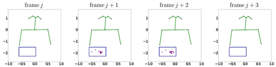
Figure 1.
Example of the fragmentary nature of the keypoint data, where coordinate values for a forearm and hand are missing in two of four consecutive frames from an example sequence. Each plot represents a single frame of keypoint x- and y-axis coordinate values from a sequence. Skeleton joints have been superimposed onto all frames to illustrate the relative positions of the visible human landmarks. Keypoints for the ears, eyes, nose, neck, shoulders, and elbows are easily identifiable. The overlaid blue boxes indicate the x–y plane location of the keypoint coordinate values that appear briefly in two of the frames.
Data standardisation, or in machine learning parlance, normalisation, refers to preprocessing techniques that put data points within an increasingly overlapping interval (e.g., ), and is often viewed as an essential step in optimising the performance of machine learning models [93]. Example benefits of normalisation include improving numerical stability of models and speeding up training such that the model is not required to functionally learn the differences in scale, as well as common patterns, across the dataset. This applies to preprocessing unseen data in the wild during inference as much as it does when learning a model.
The keypoint coordinate values in WLASL appear to be the raw values produced by OpenPose. It is self-evident that keypoints extracted from signers who appear larger in the frame will produce a different scale of values to those who appear smaller, and perhaps to a lesser extent, camera lens focal length and intrinsic lens distortion will also impact on the uniformity of video sequences, although the latter is likely to have a negligible effect. Furthermore, it is evident that signers who are at different locations within the frame will produce offset keypoint values because OpenPose reports these values relative to the origin of the video frame, which is one of the corners. To illustrate a clear example of both differences in scale and a slight offset in position, Figure 2 shows two overlaid frames extracted from two different video sequences. The two frames are cropped at the same location within the video at full resolution and clearly show a shift in scale and origin. This can be thought of as being additional (and superfluous) information to model.
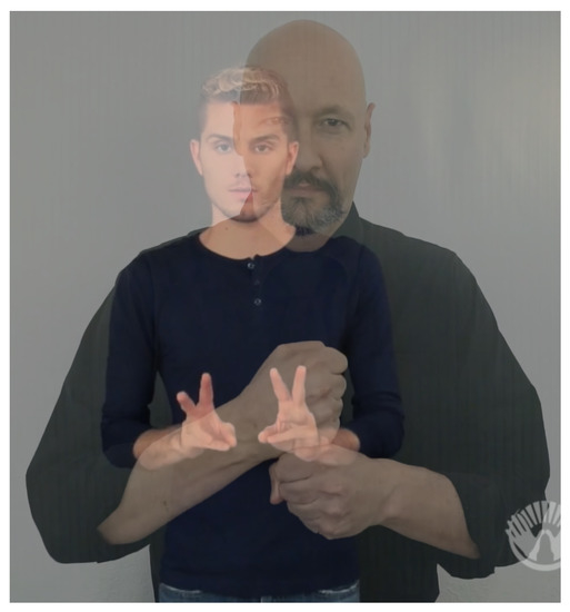
Figure 2.
Two overlaid frames extracted from two different video sequences that demonstrate difference in raw data scale and position. Images reproduced with permission, © William G. Vicars (http://lifeprint.com (accessed on 20 March 2023)) and © Start ASL (http://www.startasl.com (accessed on 20 March 2023)).
Figure 3 shows plots of the maximum x- and y-axis keypoint coordinate values taken from a representative sample of 400 sequences. The range of maximum values, including clear outliers (two of which are extreme along the y-axis), strongly suggests that normalising the data would be beneficial. Although not reported to any great depth here, we did run a short comparison study of raw versus normalised data on like-for-like experiments (i.e., the same model architecture, parameters, fixed random number generator seed, etc.) with only 10 sign classes for expediency. We found the experiments with normalised data realised a mean increase in top-1 classification accuracy of approximately 5% on the test dataset split, justifying the decision to apply our normalisation technique. We therefore normalise all data this way for all experiments.
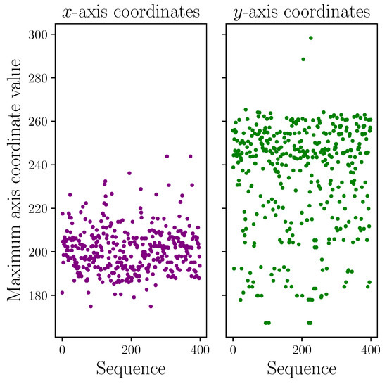
Figure 3.
Maximum x- and y-axis keypoint coordinate values taken from a representative sample of 400 sequences illustrating the range in maximum values.
There are many ways to normalise data. We take, what we believe to be, a novel approach to normalisation for sign language recognition, and try to standardise the size of every signer. We carry this out with the intention of preserving the full range of articulation for signs that require, say, larger arm motion, which is in contrast to signs that are closer to the body. Alternative methods that, for example, scale everything to the intervals , , , and so on, will likely reduce the scale of the body pose and hand keypoints for signs that produce larger arm extensions, and conversely, inflate the scale for signs with a smaller magnitude of arm extension.
We normalise the keypoint coordinate values per sequence to try to enforce a level of uniformity across the entire dataset. We take the mean x-axis distance between the left and right shoulders (body pose keypoints 2 and 5) for all frames with valid keypoint data in a given sequence, and scale every keypoint x-axis coordinate in that sequence such that the mean distance between the left and right shoulders is unity. For the y-axis coordinates, we perform the same operation but using the mean y-axis distance between the neck and nose (body pose keypoints 0 and 1), which we also set to unity. Note that the normalisation distances are axis-aligned, rather than, say, Euclidean distances.
More formally, using zero-based indexing and given I sequences of isolated signs, each sequence, , belonging to the set of all sequences, S, comprises of frames up to the maximum number of frames for all sequences in the dataset, J, and can be described as
where each isolated sign sequence has a corresponding class
where the number of classes, K, depends on the experiment being conducted. Using this definition, a given x-axis coordinate value of a keypoint position in sequence frame , denoted by , is scaled as
where is the mean x-axis coordinate value (excluding values with no valid data) of the first normalising keypoint across the entire sequence, is the corresponding value for the second normalising keypoint, and is the mask (1 or 0) indicating that this value is non-zero. Likewise, the corresponding y-axis coordinate is scaled as
where the symbols and indices follow the same convention.
Finally, we translate all keypoints for a given sequence to place the origin at the mean x- and y-axis coordinate value for the nose (keypoint 1) across that sequence. We again apply a mask to ensure the undetected keypoint values remain at the origin. Formally, a given x- or y-axis coordinate value of a keypoint position in sequence frame , denoted by , is translated to the new origin as
where is the mean value for the new origin keypoint, again using the same convention, but where the subscript represents either x or y. We do not preprocess the dataset in any way beyond this standard normalisation, which is detailed in Algorithm 1.
| Algorithm 1 Data normalisation algorithm | |
| Require: data | ▹ [sequences, frames, keypoints, x or y value] e.g., [64, 203, 54, 2] |
| Require: mask | ▹ same shape as data, specifies keypoints with valid values |
| 1: function NORM(data, mask) | |
| 2: for do | |
| 3: | ▹ Mean x value of scaling kp 0 |
| 4: | ▹ Mean x value of scaling kp 1 |
| 5: | ▹ Mean y value of scaling kp 0 |
| 6: | ▹ Mean y value of scaling kp 1 |
| 7: | ▹x distance of mean scaling kps |
| 8: | ▹y distance of mean scaling kps |
| 9: | ▹ Norm. to mean scaling kp distances |
| 10: | ▹ Mean x value of new origin kp |
| 11: | ▹ Mean y value of new origin kp |
| 12: | ▹ Translate kps to new origin |
| 13: end for | |
| 14: return data | |
| 15: end function | |
Following Li et al. [85] and Dafnis et al. [39], we programmatically split the data into training, validation, and test sets by class using the ratio . This helps balance the distribution of classes across the sets (but not the number of examples per class, which is unbalanced in WLASL), e.g., for a given class that has 6 examples, we allocate 4 examples to the training set, and 1 example to each of the validation and test sets. Taking every entry in WLASL-alt as the new catalogue index, including entries labelled as left-hand dominant, we filter out classes with fewer than 6 examples. We construct a tensor per dataset split by concatenating the extracted keypoints from the body pose, left and right hand groups by their x- and y-axis coordinate values for every frame in each example sequence. That is to say, a single frame of any given sequence is represented by 2 fixed vectors of the keypoints for that frame, grouped by x- and y-axis coordinate values (this simplifies the normalisation routine). Subsequently, a sequence is an ordered tensor of the respective frames. Finally, a dataset split is the tensor containing all respective sequences.
We pad each sequence with zeroes to a fixed length of 203 frames for the keypoint x- and y-axis coordinate values, which is the maximum sequence frame length. We do not add special token values to indicate the start or end of a sequence. Nor do we use a special token value to indicate padding, i.e., padded and no-data values are identically zero. The resultant tensors for each dataset split have the shape
where for example, the training dataset split tensor has the shape
The dataset splits are summarised in Table 3. Our experiments use subsets of these dataset splits, taking n classes with the greatest number of examples per class, depending on the experiment. These experiment data splits are listed in Table 4.
Table 3.
Dataset splits generated in this study.
Table 4.
Experiment dataset splits showing number of examples per split per number of classes.
2.2. Model
Since the introduction of transformer neural networks [18], they have been increasingly used to model many systems, most notably for applications involving natural language processing (NLP) and more recently for vision [94], but as we demonstrate in this study, transformers can be further applied to numerical sequence data. The original transformer was used to translate spoken languages, which is a sequence-to-sequence task. Our task, however, is sequence classification; that is to say we aim to classify sequences of isolated, dynamic signs according to known class labels. To achieve this, we take a standard transformer and modify it to use the encoder part only.
A transformer encoder consists of one or more encoder layers, where, in the case of multiple layers, the output from each layer is fed into the next. An encoder layer contains a multi-headed attention mechanism followed by a position-wise fully connected feed forward network. Both the attention mechanism and feed forward network are bounded by residual connections and followed by layer normalisation [95]. The residual connections help preserve some of the original input signal at various stages in the process. The processing pipeline for a single encoder layer is shown in Figure 4. The task of the transformer encoder is to take an input sequence and turn it into a latent space representation that encodes information about the relationships between the ordered parts of the input, while sharing context with other sequences it processes via the learned model parameters; in short, it projects the input into an embedded feature space.
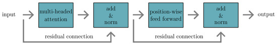
Figure 4.
High level processing pipeline of a single transformer encoder layer.
Drawing inspiration from information retrieval systems, the input embeddings are turned into queries, keys, and values that each have their own learnable parameters. The attention mechanism allows the encoder to learn semantic relationships between ordered inputs, with each having a configurable, but identical, number of heads; hence the term multi-headed attention. The query, key, and value embeddings representing each ordered item in the input sequence are split and distributed evenly across those attention heads. This can be thought of as providing each attention head an equal, but different, portion of the representation of each input in the sequence. Note that a single attention head is just a special case where the process of dividing across the heads means the lone head receives all of the embeddings.
It is a fact that transformers are position equivariant [18]. For modelling sequence data, as is the case with sign language, order is important. To alleviate this problem, positional information is injected by adding a value to each input. This value depends on the sequence position of each input and provides the model with a notion of order that it can learn. The original transformer architecture uses a fixed positional encoding, , which provides a real scalar per-input embedding dimension at position j up to a predefined maximum sequence length, J. These positional encoding scalars are derived from sinusoidal functions. For input values appearing at even positions in a sequence, these are given by
and for those at odd positions,
In both of these functions, j is the position in the sequence for a given input, i.e., , and is the dimension of the positional encoding. In other words, this maps a sinusoid to each positional encoding dimension. The value a = 10,000 was chosen by the original transformer authors because it helped balance model performance when dealing with both short and long sequences. Nevertheless, there are alternative ways to inject positional information into the input to produce ordered embeddings [96]. For ease of implementation, for the encoder-only transformer, we adopt a learned positional encoding using PyTorch’s Embedding class [97]. We generate 108 positionally encoded embedding values per sequence frame, which are added identically to each sequence in a batch.
Our transformer encoder is initialised with a configurable number of encoder layers, where every layer is identically configured according to the parameters listed in Table 5. As with the number of encoder layers and number of attention heads, other hyperparameters can potentially further optimise the model. In the encoder, we use the ReLU activation function, which is the rectified linear unit, and is defined as
which clamps negative values to zero. The same dropout probability is applied to all fully connected feed forward layers within the encoder. The fully connected feed forward layers are configured with dimension , which is essentially an arbitrary (but configurable) choice. Setting would produce a bottleneck effect, which could potentially help reduce overfitting during training. Conversely, setting would theoretically expand the feature space, helping the model learn more complex latent relationships in the data. With , as is the case in our configuration, the dimensionality of the feature space is preserved within the encoder layer.
Table 5.
Encoder layer parameters.
During training, validation and testing, we iterate through the dataset using random batching, only completing an epoch when every example in the respective dataset split has been seen by the model at least once.
Before passing a batch of data through the encoder, the input values are scaled by , where , the number of keypoint x- and y-axis coordinate values. This not only helps prevent the positional encoding from swamping the input signal, but it also helps the model to learn efficiently by preventing the positional encoding being too small a value in comparison. We experimented with other scaling factors and found scaling the input by to work well at balancing these values for this task.
The learned positional encoding is then added element-wise to the input values, which produces the input embeddings. Dropout is applied to the input embeddings according to a probability hyperparameter, which we set to throughout. The input embeddings are subsequently passed through the encoder to produce a latent representation of the same dimension as the input. After the encoder, this dimension is reduced by taking the mean value over the frame (e.g., time) axis, yielding scalars per sequence in the batch. These 108 values are further reduced or expanded to the required number of class predictions by passing them through a fully connected feed forward layer [98], which applies the linear transformation , where x is the encoder output, is the transpose of a learnable weight matrix, b is a learnable bias, and y is the resultant output. To convert the output to logits representing the class predictions, we apply the LogSoftmax function [99], which is defined as
for some class prediction , which outputs on the interval . The softmax function has the effect of amplifying larger values while suppressing smaller values (see Figure 5). These class predictions are passed into our objective function along with the ground truth class labels. We use categorical cross entropy loss [100], which combines LogSoftmax and negative log likelihood loss, to obtain a single loss value for the batch, which we accumulate per epoch. During the training loop, we compute the gradients and update the model weights using the Adam optimiser [101], initialised with the parameters listed in Table 6.
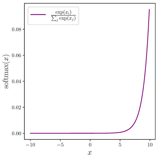
Figure 5.
Softmax function plotted over an arbitrary interval showing how it amplifies larger values of in the input x while suppressing smaller values.
Table 6.
Adam optimiser parameters.
Once per epoch, we calculate the mean loss from the accumulated batch losses, and after the training loop has completed, we perform a step on the learning rate scheduler, which we choose to be CosineAnnealingWarmRestarts [102], initialised with and otherwise default parameters.
We convert the output prediction logits, which we now define as y, to a probability distribution, , that is the predicted class probabilities for K classes, lying on the interval . This is carried out using the exponential function
so that
The predicted class probabilities and the ground truth class labels allow us to calculate top-k accuracy per epoch, where . We subsequently take a model checkpoint based on two separate performance metrics: the validation loss and the validation accuracy. For the validation loss, we take a model checkpoint if the mean batch loss for an epoch is less than the previous best performing (i.e., lowest) mean batch loss value. Likewise, we take a model checkpoint if the top-1 accuracy on the validation set is increased.
We run for 200 epochs to allow the models to converge (or overfit), after which we test using both best performing checkpoint models (based on validation loss and accuracy). We implement early stopping if both the training set accuracy and the validation top-1 accuracy reach 1.0; although in practice, this has yet to happen. A topology of the model architecture training loop for a single iteration is shown in Figure 6.
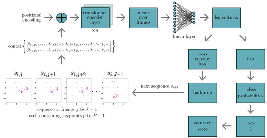
Figure 6.
Model and training loop topology for a single iteration of the sign language recognition encoder-only transformer. This diagram shows the process for a hypothetical training loop sequence batch size of 1 starting with sequence .
2.3. Model Regularisation
We perform no model regularisation, including data augmentation, in this study. Instead we choose to focus on the base architecture as a means to model and optimise the classification task, and leave regularisation to a future study to measure the impact various hyperparameters have on model performance.
2.4. Experimental Setup
All experiments were conducted in a virtual machine (VM) running on the HILDA HPC at DARTeC [103]. The VM runs on an Intel Xeon Gold 6258R with 112 CPUs and 377 GiB RAM, and 4 NVIDIA A100s each with 40 GiB RAM. Experiments were generally run in parallel batches of 4, with a single experiment per GPU. The VM operating system is Ubuntu Linux 20.04.4 LTS. The major libraries used to train and evaluate all models are Python 3.8.10, PyTorch 1.9.0+cu111, and NumPy 1.21.4.
2.5. Experiments
We began by establishing a baseline model architecture for the optimal number of encoder layers. We conducted 5 groups of 8 repeat experiments (a group per number of encoder layers), using normalised keypoint data, for a total of 40 experiments. All baseline experiments were initialised without setting the random number generation seeds, which allows us to measure the spread of model performance, and therefore quantify the standard error of the mean, and the related uncertainty, across groups of experiments. It also allows us to measure the impact random initialisation has on performance in this deep learning task. All parameters were fixed except the number of encoder layers. We limited the sign classification task to 10 classes to enable faster iteration compared to experiments with a larger number of classes. The parameters used are listed in Table 7 and the experiment dataset splits per class count are listed in Table 4.
Table 7.
Encoder layer baseline experiment hyperparameters.
With a baseline for the number of encoder layers established, we proceeded to determine the optimal number of attention heads. We did this by keeping all parameters fixed, as per Table 7, but varying the number of attention heads instead of layers. We performed 6 groups of 8 sign classification experiments with the number of attention heads, , fixed per experiment group, on 4 groups of sign classes, , for a total of 192 experiments. In total, 224 baseline experiments were conducted.
Accuracy results quoted with an associated uncertainty are calculated as
where
is the standard error of the mean, is the standard deviation, and n is the number of experiments. In all experiments, Test-A refers to the best-performing model based on the accuracy metric, and Test-L to the best performing model based on the loss metric.
3. Results
First, we report the results of the baseline experiments to determine the optimal number of transformer encoder layers for the sign language recognition task, using 10 sign classes. Because the number of learnable model parameters is directly related to the number of encoder layers (all else being equal, except for the number of attention heads, which does not influence the number of model parameters), we also include those figures here. Mean top-1 accuracy results are listed in Table 8 and plotted in Figure 7, which presents the same data as functions of encoder layers and number of model parameters, respectively.
Table 8.
Mean top-1 accuracy results for optimal number of encoder layers and number of model parameters for baseline experiments with 10 classes.
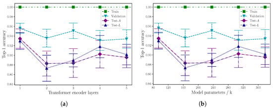
Figure 7.
Mean top-1 accuracy results as a function of (a) number of encoder layers, and (b) number of model parameters, for baseline experiments with 10 classes.
Next, we report the results of the baseline experiments to determine the optimal number of attention heads per group of classes. Top-1 accuracy results are listed in Table 9 and plotted in Figure 8.
Table 9.
Mean top-1 accuracy results for encoder attention heads for baseline experiments with 10, 50, 100, and 300 classes. Each row gives the mean result from eight repeat experiments.
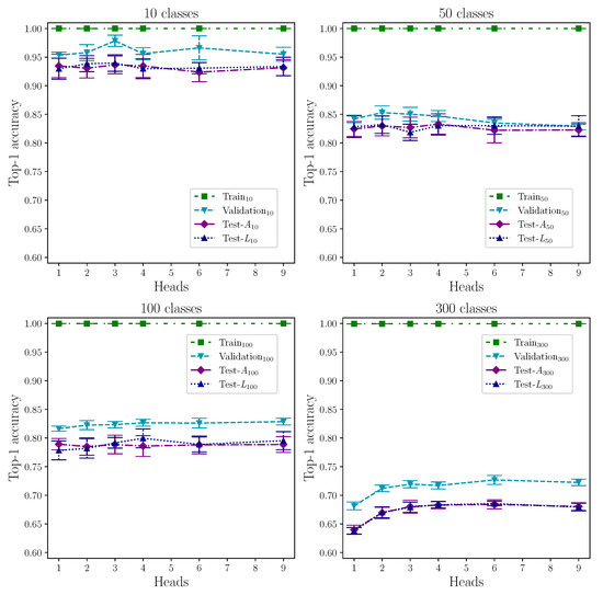
Figure 8.
Top-1 accuracy results for attention heads baseline experiments with 10, 50, 100, and 300 classes.
We present the model configurations that achieve the best test set top-k accuracy in Table 10. These results include the performance metric that achieves the best score for each top-k accuracy, which is reported as A for the accuracy-based checkpoint metric, L for the loss-based equivalent, or same in the event that both results are equal.
Table 10.
Mean top-1, top-5, and top-10 test set accuracy results for best performing model configurations from experiments with 10, 50, 100, and 300 classes, showing number of attention heads, best performance metric, and difference in accuracy between performance metrics.
As each experiment result is the mean accuracy from eight separate, identically configured but randomly initialised, experiments, we report the accuracy range and uncertainty to provide insight into model variability between experiments. These results are listed in Table 11.
Table 11.
Range and uncertainty in top-1 test accuracy for repeated experiments per configuration and performance metric, where: ; is the standard error of the mean; and is the standard deviation.
Table 12 shows the top-1, top-5, and top-10 minimum, mean, and maximum test accuracy results from our best performing model configurations for each of the data splits by sign count, where the best model configuration is taken as that which scores the highest mean accuracy. We include all three of these values to provide insight into the range of performance for a given so-called best model configuration when randomly initialised. That is to say, the model configuration that performs best on average after repeat experiments. We note that this means we may not report the absolute maximum accuracy scores across all model configurations; in this study, we are most interested in model configurations that generally perform well under conditions brought about by random initialisation. We also include our results along with those from other models, but it is important to note that this is indicative of relative performance only. We use WLASL-alt, the modified version of WLASL, as the basis of our dataset which uses the exact same keypoint data as WLASL, but it does have improved glosses, which likely affect the outcome. In the absence of any results that quote the same class numbers and data splits, we use these for cautious comparison.
Table 12.
Best top-1, top-5, and top-10 test accuracy results for human pose-estimation-based sign language recognition using WLASL-based data. For our results, we report the minimum, mean, and maximum accuracy scores for the best performing model configuration measured by highest mean accuracy. Note that our results stem from WLASL-alt, which has improved glosses, and the results are, therefore, indicative of relative performance. We omit the uncertainty for our mean values.
4. Discussion
4.1. Model Performance
We successfully perform sign language recognition on isolated, dynamic signs across a range of class sizes using an encoder-only transformer and a novel data normalisation technique, with no data augmentation or model regularisation. The results are as expected insofar as performance decreases as the number of classes is increased. The same applies to the three dataset splits, with performance being greatest on the training set, followed by the validation set, then the test set splits. The goal—like the majority of similar machine learning classification tasks—however, is to maximise performance on the test set, which is a better reflection of model generalisation, and therefore performance in the wild; performing well on dataset splits other than the test set is an insufficient indicator of real-world performance.
Our attempt to determine an optimal model architecture by number of encoder layers identifies a single layer as being optimal over multiple layers, up to a maximum of five. In Figure 7, the error bars suggest a layer count greater than one offers no performance benefit on the test set accuracy, though this is marginal for the case of four encoder layers. Despite this, the overall trend appears to be a decrease in accuracy as the number of layers increase. Table 8 shows that a single layer yields the highest accuracy on both performance metrics. It should be noted, however, that we can only state this for the case of modelling 10 sign classes. Repeating the experiments with different layer counts for greater class sizes would provide more insight.
Conversely, as Figure 8 shows, we were unable to determine the optimal number of heads for a single layer for under 300 classes because they all perform equally well, within the quoted uncertainty. In the case of 300 heads, however, there is a stark rise in performance between 1 and 2 attention heads of approximately . This almost certainly reflects the increase in dataset complexity through the additional classes that marks the crossing of a threshold. Taking into account the measured uncertainty, the increase in performance appears to plateau after two heads. We can tentatively predict that the number of heads required to achieve the best accuracy will increase monotonically with significant increases in number of classes, within the limits of the model. This relationship between dataset complexity and model complexity, through the number of attention heads, suggests the same might be true with the number of layers in the transformer encoder. Again, empiricism is the key here. For class sizes , we establish that a single attention head within a single encoder layer is sufficient to model sign language to a high accuracy using our method. Figure 9 shows model performance for top-1, top-5, and top-10 across the range of classes used in our experiments.
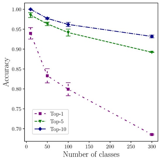
Figure 9.
Best mean accuracy per class by top-k result for .
Moreover, the fact that the top-1 accuracies (shown in Table 9) on the training set reach (or just below) clearly demonstrates that our encoder-only transformer is capable of learning a model of the dataset. We can confidently state that the model is overfitting the data, which means it begins to memorise the representations of the sequences, including any inherent noise. This is unsurprising given the low number of examples per class split; Table 4 shows that for 10 classes, there are a mere 282 training and 68 validation set examples, and for the upper limit of 300 classes, there are only 4302 and 950 examples, respectively. By deep learning standards, these numbers are miniscule. Considering that there are no data augmentation techniques present in this study, random batching (i.e., an epoch completes only when every example has been seen at least once) may offer some regularisation effect. We anticipate that standard regularisation techniques, both via the model (through, e.g., embedding or encoder dropout, introducing a bottleneck to reduce the features, etc.) and data augmentation would help reduce overfitting and improve validation and test set accuracy. As we only take model checkpoints when a performance metric has been improved upon, we can be confident that, in this instance, overfitting is not to the detriment of validation accuracy, and therefore by extension, test accuracy.
Our study makes no use of the OpenPose confidence score for each of the estimated keypoint coordinates. Given that OpenPose can incorrectly report keypoints, particularly for keypoints corresponding to the hands, this suggests our model learns from noisy data. Model performance may be increased by improving the keypoint data in several ways, which include: filtering keypoint coordinates based on a minimum confidence score threshold as a tuneable hyperparameter; processing keypoints to attempt to correct for more obvious errors, e.g., where two values momentarily swap positions, or detecting unlikely and invalid pose configurations; including the confidence score in the model as another feature to learn, although this latter option will inflate the model size; and, conversely, reducing the number of keypoint values used for the hands, which would also reduce the model size.
We deliberately chose to include left-hand-dominant examples to increase the real-world representative power of the dataset. However, given the low number of examples, we acknowledge that they could make the task more challenging, particularly if the left-hand-dominant example resides in the test split only. Because of the low number of available examples, we made no efforts to control for balance across left-hand-dominant examples. Reflecting about the y-axis is a typical augmentation method in image classification tasks, but we would be against performing the equivalent with x-axis coordinates simply because there are signs for left and right present in the dataset, albeit not in any of our 10, 50, 100, or 300 splits.
Our choice of two separate performance metrics, in the form of accuracy and loss, is found to have negligible influence over performance outcome. This can be seen in the results listed in Table 10 where, with the exception of top-1 for 100 classes, the difference in accuracy between the two performance metrics is <. Figure 8 shows the top-1 results for 100 classes and 4 attention heads still lie within the error bars on both metrics, and we conclude the comparably large value of is not so much the outlier it initially appears to be. The similarity between both metrics is most vivid at 300 classes. This can be explained by the increased random batch count per epoch to dataset size ratio, which increases with the number of classes, as shown in Figure 10. This indicates that future studies can reasonably use either accuracy or loss as a sole performance metric for this task to produce highly comparable results.
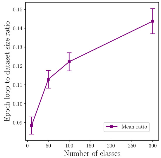
Figure 10.
Mean random batch loops per epoch to number of classes ratio showing experiments with greater numbers of classes require more random batch iterations. Any regularisation effect produced by this is likely amplified with increased class count.
Despite the random batching mechanism we employ likely having a regularisation effect, it is also possible that it can contribute to the model overfitting. It is common when using multiple-pass type techniques to find a balance so the model is exposed to enough data to learn patterns to be able to generalise, but not so much it begins to memorise. Lack of resources prevent us from being able to test the regularisation-overfitting-balance question in this study, but we choose this method of batching to facilitate the introduction of on-the-fly data augmentation in later studies with no system architecture changes, which should have a positive effect on performance.
Although our use of WLASL-alt as the basis for our experiments means it is not possible to directly compare our results with those of other models, we can, however, perform some indirect comparison. Table 12 shows our models outperform others on similar tasks, and in most cases by a substantial margin, but we acknowledge this could be partially the result of using what is simply a better version of the dataset.
4.2. Model Training Practicalities
Figure 11 shows the epochs that produced the best score for both the accuracy and loss performance metrics. That is to say, it indicates the epochs that were checkpointed for each metric, and hence used in the test evaluation to produce the accuracy scores. Making the assumption that conducting enough experiments would produce a normal distribution, the overlaid probability density function suggests the upper tail would include experiments where the best performing epoch occurs in excess of the arbitrary 200 epoch limit we chose for practical reasons. The peak around 130 epochs strongly suggests the majority of experiments would produce a best-performing model within the 200 epoch limit. Extrapolating the upper tail—marked with a green dashed line—shows approximately 250 epochs meets the limit of a sufficient training length to capture the vast majority of inliers, although this is a conservative estimate. Given sufficient resources, this could be determined empirically.
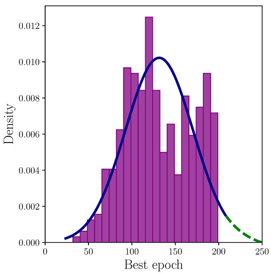
Figure 11.
Best epoch by accuracy and loss performance metrics after 200 epochs with probability density function overlaid in blue. The green dashed line represents the extrapolated upper tail.
To illustrate the required time to conduct individual experiments in this study, Figure 12 shows the mean time to complete an experiment of 200 epochs plotted against the number of classes in each experiment. We find this relationship to be approximately . Note that this is the time to complete 200 epochs on our VM (which has shared resources such as GPUs, etc.) using the random batching method which is inefficient compared with, say, taking sequential slices of the data per batch preloaded onto a GPU. This time to complete 200 epochs is inflated somewhat because it includes auto-generated plots that happen every epoch or, in the case of confusion matrices, every n epochs, all of which adds to the time. From this plot, it is possible to estimate the time required to conduct further experiments on larger class sizes.
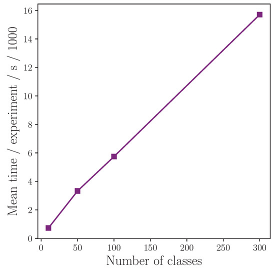
Figure 12.
Mean time to complete an experiment of 200 epochs as a function of number of classes, showing approximate linear relationship.
In practice—particularly in an industrial setting—one would retrain a model many times without fixed random number generator seeds and take the best performing model. Fixing seeds is useful for reproducing results, but this has limited utility across computer architectures, e.g., running the exact same experiment, including fixed seeds, on HILDA and another computer yields different results. It is important to understand the range of results that can be produced from repeat experiments to help provide estimates to the number of experiments required to achieve performance that approaches the theoretical optimum. In our case, it is impractical to conduct many experiments per configuration, so we set the number to eight, and in the interest of reporting realistic results, we also take the mean and worst performances from these eight experiments, and not just the best score. Table 11 shows the range of results, which can only remain the same or increase with the number of experiments, n, but one would naturally expect a true range to be asymptotically approached as , but practical limitations exist.
It is clear that the range across repeat experiments is large for our model. The maximum range of over occurs on the experiment with 50 classes and 6 attention heads. There appears to be no correlation between experiment configuration (i.e., number of attention heads) and the range of accuracies achieved. Such a high range is an indicator of model instability and sensitivity to random variable changes. This is likely a symptom (and another sign) of the model overfitting the training data. As well as helping diagnose problems in machine learning models, analysing the variability of results also reinforces the importance of repeating experiments without fixed random number generator seeds and reporting mean results with appropriate uncertainties. This has implications for reproducing published models and results.
4.3. Model Architecture and Parameters
Perhaps most surprising is the ability of our model to perform well on this classification task despite having so few parameters. To put it in context, whereas SPOTER [89] and I3D [86] have 5.92 million and 12.35 million parameters, respectively, our single layer encoder-only transformer model has 94 thousand parameters (see Table 8). This means our model can be trained on a relatively modest GPU with 4 GiB RAM, and subsequently deployed to hardware for inference with even lower memory capacity.
Increasing the number of attention heads does not increase the number of learnable parameters. However, every additional encoder layer in our model increases the number of parameters by 71,064, but this number can be reduced by rationalising the number of keypoints used in each hand, which are frequently obscured and misplaced by OpenPose. With no performance gain on smaller class numbers, it is self-evident that a single layer is preferable for these applications because it reduces the hardware requirements.
4.4. Normalisation
We found our normalisation technique to work well for this task. We made an arbitrary choice of keypoints to normalise to along the x and y axes. Our choice of keypoint to centre on was somewhat inspired by evidence that shows expert signers focus on the central part of the face of their conversation partner when signing [104]. We did not test relative performance as a function of central keypoint selection, but we believe our choice of normalisation coordinates (i.e., the shoulders) to be the best choice on logical grounds. Again, this remains an open question.
Beyond normalisation, we believe the fact we do not preprocess the dataset in any other way gives our model the advantage for applying it to sign language recognition technology in the wild. This statement holds even if augmentation is introduced because it is not common practice to augment test data.
5. Conclusions
In this article, we present a study on modelling ASL using an encoder-only transformer and human pose estimation keypoint data derived from WLASL-alt, an improved version of the WLASL dataset. Using a novel normalisation technique, we perform sign language recognition on 10, 50, 100, and 300 classes of isolated, dynamic signs, and conduct extensive analysis on the impact fundamental model architecture has on performance; namely the number of encoder layers and attention heads. We evaluate our models during training using two different performance metrics based on accuracy and loss, and we find them to produce similar outcomes within the measured uncertainty, with no clear preferred metric for this task. We demonstrate that a very small model, by parameter count, is capable of modelling sign language to a high accuracy for limited vocabulary sizes.
We compare our results with other studies that perform sign language recognition on the same base dataset. However, we acknowledge that, because we use an improved version of WLASL, these comparisons are indicative only. Because of the flaws identified by Dafnis et al. [39], we discourage further use of the WLASL dataset in its original form, and actively promote the use of the improved WLASL-alt dataset. To support this, we have also published the dataset splits used in this study at https://github.com/ltwoods/msl (accessed on 20 March 2023).
We limit our maximum class count to 300 classes because of the time taken to perform a single experiment and the requirement to conduct multiple experiments per configuration, which we find to be prohibitively long. While reduced vocabulary models have clear utility in specific, controlled settings, for generalised sign language recognition technology to be deployed in the wild, it would need to accommodate for many more sign classes (e.g., approaching 10,000 sign classes for ASL), which goes beyond the mere 300 classes we use in this study. This is both a challenge for model creation as well as dataset curation. Given our selection criteria, detailed in Section 1.3, the dataset splits we extract from WLASL-alt reduces the number of classes provided in the WLASL dataset below the original 2000, which itself falls short of the number of classes required for real-world sign language recognition.
In Section 4, we offer suggestions of related aspects that warrant study. In addition, here we stress the importance non-manual markers play in providing richness and complexity to sign language. Non-manual markers include things such as head position, eyebrows, mouth shape, body shift, and so on. There are no OpenPose face keypoints in the WLASL dataset, and the pose keypoints that include some facial landmarks are extremely limited in that only the central positions of the eyes, ears, and nose are provided. This means the important articulators such as eyebrows and mouth shape are omitted. Eyebrow configuration can differentiate questions from statements, and mouth shapes can help distinguish between signs with common hand configurations as well as provide extra context or emphasis. It is essential that these non-manual markers are included for sign language recognition to generalise to many more signs. This is one area where appearance-based techniques have an advantage.
Beyond the relative simplicity of the model architecture, another notable outcome of this study is that we demonstrate that an encoder-only transformer is capable of modelling sign language to a high accuracy without the aid of data augmentation or explicit model regularisation techniques; techniques that, it is anticipated, will improve performance further.
Author Contributions
Conceptualization, L.T.W. and Z.A.R.; methodology, L.T.W.; software, L.T.W.; validation, L.T.W.; formal analysis, L.T.W.; investigation, L.T.W.; resources, Z.A.R.; writing—original draft preparation, L.T.W.; writing—review and editing, L.T.W. and Z.A.R.; visualization, L.T.W.; supervision, Z.A.R.; project administration, Z.A.R.; funding acquisition, L.T.W. and Z.A.R. All authors have read and agreed to the published version of the manuscript.
Funding
This research is funded by Leidos Industrial Engineers Limited.
Data Availability Statement
The WLASL dataset is available at https://dxli94.github.io/WLASL/ (accessed on 20 March 2023). The WLASL-alt dataset is available at https://dai.cs.rutgers.edu/dai/s/wlasl (accessed on 20 March 2023). The dataset splits used in this study are available at https://github.com/ltwoods/msl (accessed on 20 March 2023).
Acknowledgments
The authors would like to thank William G. Vicars of http://lifeprint.com and Jessica Mayer of http://www.startasl.com for granting and arranging for permission to reproduce their images. The authors would also like to thank George Yazigi for bringing HILDA to life, and the reviewers and editors for their insightful comments.
Conflicts of Interest
The authors declare no conflict of interest. The funders had no role in the design of the study; in the collection, analyses, or interpretation of data; in the writing of the manuscript; or in the decision to publish the results.
Abbreviations
The following abbreviations are used in this manuscript:
| ASL | American Sign Language |
| BERT | Bidirectional Encoder Representations from Transformers |
| BSL | British Sign Language |
| DSG | German Sign Language |
| GRU | gated recurrent unit |
| HCI | human–computer interaction |
| I3D | Inflated 3D ConvNet |
| NLP | natural language processing |
| ReLU | rectified linear unit |
| SPOTER | Sign POsebased TransformER |
| VM | virtual machine |
| WLASL | Word-level American Sign Language dataset |
| WLASL-alt | Word-level American Sign Language alternative dataset |
References
- Vamplew, P.W. Recognition of Sign Language Using Neural Networks. Ph.D. Thesis, University of Tasmania, Hobart, Australia, 1996. [Google Scholar]
- Starner, T.; Weaver, J.; Pentland, A. Real-Time American Sign Language Recognition Using Desk and Wearable Computer Based Video. IEEE Trans. Pattern Anal. Mach. Intell. 1998, 20, 1371–1375. [Google Scholar] [CrossRef]
- Stokoe, W.C. Sign Language Structure: An Outline of the Visual Communication Systems of the American Deaf; University of Buffalo: Buffalo, NY, USA, 1960. [Google Scholar]
- Tamura, S.; Kawasaki, S. Recognition of Sign Language Motion Images. Pattern Recognit. 1988, 21, 343–353. [Google Scholar] [CrossRef]
- Vogler, C.; Sun, H.; Metaxas, D. A Framework for Motion Recognition with Applications to American Sign Language and Gait Recognition. In Proceedings of the Workshop on Human Motion, Austin, TX, USA, 7–8 December 2000; pp. 33–38. [Google Scholar] [CrossRef]
- Kim, S.; Waldron, M.B. Adaptation of Self Organizing Network for ASL Recognition. In Proceedings of the 15th Annual International Conference of the IEEE Engineering in Medicine and Biology Society, San Diego, CA, USA, 31 October 1993; p. 254. [Google Scholar] [CrossRef]
- Waldron, M.B.; Kim, S. Isolated ASL Sign Recognition System for Deaf Persons. IEEE Trans. Rehabil. Eng. 1995, 3, 261–271. [Google Scholar] [CrossRef]
- Vogler, C.; Metaxas, D. Parallel Hidden Markov Models for American Sign Language Recognition. In Proceedings of the Seventh IEEE International Conference on Computer Vision, Kerkyra, Greece, 20–27 September 1999; Volume 1, pp. 116–122. [Google Scholar] [CrossRef]
- Kadir, T.; Bowden, R.; Ong, E.J.; Zisserman, A. Minimal Training, Large Lexicon, Unconstrained Sign Language Recognition. In Proceedings of the British Machine Vision Conference, Kingston, UK, 7–9 September 2004; Hoppe, A., Barman, S., Ellis, T., Eds.; pp. 96.1–96.10. [Google Scholar] [CrossRef]
- Cooper, H.; Bowden, R. Sign Language Recognition Using Linguistically Derived Sub-Units. In Proceedings of the Language Resources and Evaluation Conference Workshop on the Representation and Processing of Sign Languages: Corpora and Sign Languages Technologies, MCC, Valetta, Malta, 17–23 May 2010; pp. 1–5. [Google Scholar]
- Theodorakis, S.; Pitsikalis, V.; Maragos, P. Model-Level Data-Driven Sub-Units for Signs in Videos of Continuous Sign Language. In Proceedings of the 2010 IEEE International Conference on Acoustics, Speech and Signal Processing, Dallas, TX, USA, 14–19 March 2010; pp. 2262–2265. [Google Scholar] [CrossRef]
- Pitsikalis, V.; Theodorakis, S.; Vogler, C.; Maragos, P. Advances in Phonetics-Based Sub-Unit Modeling for Transcription Alignment and Sign Language Recognition. In Proceedings of the IEEE Computer Society Conference on Computer Vision and Pattern Recognition Workshops, Colorado Springs, CO, USA, 20–25 June 2011; pp. 1–6. [Google Scholar] [CrossRef]
- Cooper, H.; Ong, E.J.; Pugeault, N.; Bowden, R. Sign Language Recognition Using Sub-Units. J. Mach. Learn. Res. 2012, 13, 2205–2231. [Google Scholar] [CrossRef]
- Koller, O.; Ney, H.; Bowden, R. May the Force Be with You: Force-aligned Signwriting for Automatic Subunit Annotation of Corpora. In Proceedings of the 2013 10th IEEE International Conference and Workshops on Automatic Face and Gesture Recognition (FG), Shanghai, China, 22–26 April 2013; pp. 1–6. [Google Scholar] [CrossRef]
- Zhang, J.; Zhou, W.; Xie, C.; Pu, J.; Li, H. Chinese Sign Language Recognition with Adaptive HMM. In Proceedings of the 2016 IEEE International Conference on Multimedia and Expo (ICME), Seattle, WA, USA, 11–15 July 2016; pp. 1–6. [Google Scholar] [CrossRef]
- Camgöz, N.C.; Hadfield, S.; Koller, O.; Bowden, R. SubUNets: End-to-End Hand Shape and Continuous Sign Language Recognition. In Proceedings of the IEEE International Conference on Computer Vision, Venice, Italy, 22–29 October 2017; pp. 3075–3084. [Google Scholar] [CrossRef]
- Mittal, A.; Kumar, P.; Roy, P.P.; Balasubramanian, R.; Chaudhuri, B.B. A Modified LSTM Model for Continuous Sign Language Recognition Using Leap Motion. IEEE Sens. J. 2019, 19, 7056–7063. [Google Scholar] [CrossRef]
- Vaswani, A.; Brain, G.; Shazeer, N.; Parmar, N.; Uszkoreit, J.; Jones, L.; Gomez, A.N.; Kaiser, Ł.; Polosukhin, I. Attention Is All You Need. In Proceedings of the Advances in Neural Information Processing Systems; Long Beach Convention and Entertainment Center: Long Beach, CA, USA, 2017; pp. 5998–6008. [Google Scholar]
- Devlin, J.; Chang, M.W.; Lee, K.; Toutanova, K. BERT: Pre-training of Deep Bidirectional Transformers for Language Understanding. In Proceedings of the 2019 Conference of the North American Chapter of the Association for Computational Linguistics: Human Language Technologies, Minneapolis, MN, USA, 2–7 June 2019; (Long and Short Papers). Volume 1, pp. 4171–4186. [Google Scholar] [CrossRef]
- Hosemann, J. Eye Gaze and Verb Agreement in German Sign Language: A First Glance. Sign Lang. Linguist. 2011, 14, 76–93. [Google Scholar] [CrossRef]
- LeMaster, B. What Difference Does Difference Make?: Negotiating Gender and Generation in Irish Sign Language. In Gendered Practices in Language; Benor, S., Rose, M., Sharma, D., Sweetland, J., Zhang, Q., Eds.; CSLI Publications, Stanford University: Stanford, CA, USA, 2002; pp. 309–338. [Google Scholar]
- Klomp, U. Conditional Clauses in Sign Language of the Netherlands: A Corpus-Based Study. Sign Lang. Stud. 2019, 19, 309–347. [Google Scholar] [CrossRef]
- Bickford, J.A.; Fraychineaud, K. Mouth Morphemes in ASL: A Closer Look. In Proceedings of the Theoretical Issues in Sign Language Research Conference, Florianopolis, Brazil, 6–9 December 2006; pp. 32–47. [Google Scholar]
- Bragg, D.; Koller, O.; Bellard, M.; Berke, L.; Boudreault, P.; Braffort, A.; Caselli, N.; Huenerfauth, M.; Kacorri, H.; Verhoef, T.; et al. Sign Language Recognition, Generation, and Translation: An Interdisciplinary Perspective. In Proceedings of the ASSETS 2019—21st International ACM SIGACCESS Conference on Computers and Accessibility, Pittsburgh, PA, USA, 28–30 October 2019; pp. 16–31. [Google Scholar] [CrossRef]
- Emmorey, K. Language and Space (Excerpt). In Space: In Science, Art, and Society; Penz, F., Radick, G., Howell, R., Eds.; Cambridge University Press: Cambridge, UK, 2004; pp. 22–45. [Google Scholar]
- Woll, B. Digiti Lingua: A Celebration of British Sign Language and Deaf Culture; The Royal Society: London, UK, 2013. [Google Scholar]
- Quer, J.; Steinbach, M. Ambiguities in Sign Languages. Linguist. Rev. 2015, 32, 143–165. [Google Scholar] [CrossRef]
- Kramer, J.; Leifer, L. The Talking Glove. ACM SIGCAPH Comput. Phys. Handicap. 1988, 39, 12–16. [Google Scholar] [CrossRef]
- Massachusetts Institute of Technology. Ryan Patterson, American Sign Language Translator/Glove. 2002. Available online: https://lemelson.mit.edu/resources/ryan-patterson (accessed on 20 March 2023).
- Osika, M. EnableTalk. 2012. Available online: https://web.archive.org/web/20200922151309/https://enabletalk.com/welcome-to-enabletalk/ (accessed on 27 February 2023).
- Lin, M.; Villalba, R. Sign Language Glove. 2014. Available online: https://people.ece.cornell.edu/land/courses/ece4760/FinalProjects/f2014/rdv28_mjl256/webpage/ (accessed on 20 March 2023).
- BrightSign Technology Limited. The BrightSign Glove. 2015. Available online: https://www.brightsignglove.com/ (accessed on 20 March 2023).
- Pryor, T.; Azodi, N. SignAloud: Gloves That Transliterate Sign Language into Text and Speech, Lemelson-MIT Student Prize Undergraduate Team Winner. 2016. Available online: https://web.archive.org/web/20161216144128/https://lemelson.mit.edu/winners/thomas-pryor-and-navid-azodi (accessed on 20 March 2023).
- Avalos, J.M.L. IPN Engineer Develops a System for Sign Translation. 2016. Available online: http://www.cienciamx.com/index.php/tecnologia/robotica/5354-sistema-para-traduccion-de-senas-en-mexico-e-directa (accessed on 20 March 2023).
- O’Connor, T.F.; Fach, M.E.; Miller, R.; Root, S.E.; Mercier, P.P.; Lipomi, D.J.; O’Connor, T.F.; Fach, M.E.; Miller, R.; Root, S.E.; et al. The Language of Glove: Wireless Gesture Decoder with Low-Power and Stretchable Hybrid Electronics. PLoS ONE 2017, 12, e0179766. [Google Scholar] [CrossRef]
- Allela, R.; Muthoni, C.; Karibe, D. SIGN-IO. 2019. Available online: http://sign-io.com/ (accessed on 20 March 2023).
- Forshay, L.; Winter, K.; Bender, E.M. Open Letter to UW’s Office of News & Information about the SignAloud Project. 2016. Available online: http://depts.washington.edu/asluw/SignAloud-openletter.pdf (accessed on 20 March 2023).
- Erard, M. Why Sign Language Gloves Don’t Help Deaf People. Deaf Life 2019, 24, 22–39. [Google Scholar]
- Dafnis, K.M.; Chroni, E.; Neidle, C.; Metaxas, D.N. Bidirectional Skeleton-Based Isolated Sign Recognition Using Graph Convolutional Networks. In Proceedings of the 13th Conference on Language Resources and Evaluation (LREC 2022), Marseille, France, 20–25 June 2022. [Google Scholar]
- Johnston, T. Auslan Corpus Annotation Guidelines. 2013. Available online: https://media.auslan.org.au/attachments/AuslanCorpusAnnotationGuidelines_Johnston.pdf (accessed on 20 March 2023).
- Cormier, K.; Fenlon, J. BSL Corpus Annotation Guidelines. 2014. Available online: https://bslcorpusproject.org/wp-content/uploads/BSLCorpusAnnotationGuidelines_23October2014.pdf (accessed on 20 March 2023).
- Crasborn, O.; Bank, R.; Cormier, K. Digging into Signs: Towards a Gloss Annotation Standard for Sign Language Corpora. In Proceedings of the 7th Workshop on the Representation and Processing of Sign Languages: Corpus Mining, Language Resources and Evaluation Conference, Portorož, Slovenia, 28 May 2016; pp. 1–11. [Google Scholar] [CrossRef]
- Mesch, J.; Wallin, L. Gloss Annotations in the Swedish Sign Language Corpus. Int. J. Corpus Linguist. 2015, 20, 102–120. [Google Scholar] [CrossRef]
- Gries, S.T.; Berez, A.L. Handbook of Linguistic Annotation; Springer: Dordrecht, The Netherlands, 2017. [Google Scholar] [CrossRef]
- Koller, O.; Ney, H.; Bowden, R. Deep Hand: How to Train a CNN on 1 Million Hand Images When Your Data Is Continuous and Weakly Labelled. In Proceedings of the 2016 IEEE Conference on Computer Vision and Pattern Recognition (CVPR), Las Vegas, NV, USA, 27–30 June 2016; pp. 3793–3802. [Google Scholar] [CrossRef]
- Hosain, A.A.; Santhalingam, P.S.; Pathak, P.; Rangwala, H.; Kosecka, J. FineHand: Learning Hand Shapes for American Sign Language Recognition. In Proceedings of the 2020 15th IEEE International Conference on Automatic Face and Gesture Recognition (FG 2020), Buenos Aires, Argentina, 16–20 November 2020; pp. 700–707. [Google Scholar] [CrossRef]
- Mukushev, M.; Imashev, A.; Kimmelman, V.; Sandygulova, A. Automatic Classification of Handshapes in Russian Sign Language. In Proceedings of the the LREC2020 9th Workshop on the Representation and Processing of Sign Languages: Sign Language Resources in the Service of the Language Community, Technological Challenges and Application Perspectives, Marseille, France, 11–16 May 2020; pp. 165–170. [Google Scholar]
- Rios-Figueroa, H.V.; Sánchez-García, A.J.; Sosa-Jiménez, C.O.; Solís-González-Cosío, A.L. Use of Spherical and Cartesian Features for Learning and Recognition of the Static Mexican Sign Language Alphabet. Mathematics 2022, 10, 2904. [Google Scholar] [CrossRef]
- Yang, S.H.; Cheng, Y.M.; Huang, J.W.; Chen, Y.P. RFaNet: Receptive Field-Aware Network with Finger Attention for Fingerspelling Recognition Using a Depth Sensor. Mathematics 2021, 9, 2815. [Google Scholar] [CrossRef]
- Goldin-Meadow, S.; Brentari, D. Gesture, Sign, and Language: The Coming of Age of Sign Language and Gesture Studies. Behav. Brain Sci. 2017, 40, e46. [Google Scholar] [CrossRef]
- Antonakos, E.; Roussos, A.; Zafeiriou, S. A Survey on Mouth Modeling and Analysis for Sign Language Recognition. In Proceedings of the 2015 11th IEEE International Conference and Workshops on Automatic Face and Gesture Recognition (FG), Ljubljana, Slovenia, 4–8 May 2015; pp. 1–7. [Google Scholar] [CrossRef]
- Capek, C.M.; Waters, D.; Woll, B.; MacSweeney, M.; Brammer, M.J.; McGuire, P.K.; David, A.S.; Campbell, R. Hand and Mouth: Cortical Correlates of Lexical Processing in British Sign Language and Speechreading English. J. Cogn. Neurosci. 2008, 20, 1220–1234. [Google Scholar] [CrossRef]
- Koller, O.; Ney, H.; Bowden, R. Deep Learning of Mouth Shapes for Sign Language. In Proceedings of the 2015 IEEE International Conference on Computer Vision Workshop (ICCVW), Santiago, Chile, 7–13 December 2015; pp. 477–483. [Google Scholar] [CrossRef]
- Wilson, N.; Brumm, M.; Grigat, R.R. Classification of Mouth Gestures in German Sign Language Using 3D Convolutional Neural Networks. In Proceedings of the 10th International Conference on Pattern Recognition Systems (ICPRS-2019), Tours, France, 8–10 July 2019; Institution of Engineering and Technology: Tours, France, 2019; pp. 52–57. [Google Scholar] [CrossRef]
- Michael, N.; Yang, P.; Liu, Q.; Metaxas, D.; Neidle, C. A Framework for the Recognition of Nonmanual Markers in Segmented Sequences of American Sign Language. In Proceedings of the British Machine Vision Conference, Dundee, UK, 29 August–2 September 2011; British Machine Vision Association: Dundee, UK, 2011; pp. 124.1–124.12. [Google Scholar] [CrossRef]
- Antonakos, E.; Pitsikalis, V.; Maragos, P. Classification of Extreme Facial Events in Sign Language Videos. EURASIP J. Image Video Process. 2014, 2014, 14. [Google Scholar] [CrossRef]
- Metaxas, D.; Dilsizian, M.; Neidle, C. Scalable ASL Sign Recognition Using Model-Based Machine Learning and Linguistically Annotated Corpora. In Proceedings of the 8th Workshop on the Representation & Processing of Sign Languages: Involving the Language Community, Language Resources and Evaluation Conference, Miyazaki, Japan, 12 May 2018. [Google Scholar]
- Camgöz, N.C.; Koller, O.; Hadfield, S.; Bowden, R. Multi-Channel Transformers for Multi-articulatory Sign Language Translation. In Proceedings of the 16th European Conference on Computer Vision (ECCV 2020) Part XI, Glasgow, UK, 23–28 August 2020; pp. 1–18. [Google Scholar]
- Weast, T.P. Questions in American Sign Language: A Quantitative Analysis of Raised and Lowered Eyebrows. Ph.D. Thesis, University of Texas at Arlington, Arlington, TX, USA, 2008. [Google Scholar]
- Najafabadi, M.M.; Villanustre, F.; Khoshgoftaar, T.M.; Seliya, N.; Wald, R.; Muharemagic, E. Deep Learning Applications and Challenges in Big Data Analytics. J. Big Data 2015, 2, 1–21. [Google Scholar] [CrossRef]
- Von Agris, U.; Blömer, C.; Kraiss, K.F. Rapid Signer Adaptation for Continuous Sign Language Recognition Using a Combined Approach of Eigenvoices, MLLR, and MAP. In Proceedings of the 2008 19th International Conference on Pattern Recognition, Tampa, FL, USA, 8–11 December 2008; pp. 1–4. [Google Scholar] [CrossRef]
- Gweth, Y.L.; Plahl, C.; Ney, H. Enhanced Continuous Sign Language Recognition Using PCA and Neural Network Features. In Proceedings of the 2012 IEEE Computer Society Conference on Computer Vision and Pattern Recognition Workshops, Providence, RI, USA, 16–21 June 2012; pp. 55–60. [Google Scholar] [CrossRef]
- Forster, J.; Koller, O.; Oberdörfer, C.; Gweth, Y.; Ney, H. Improving Continuous Sign Language Recognition: Speech Recognition Techniques and System Design. In Proceedings of the SLPAT 2013, 4th Workshop on Speech and Language Processing for Assistive Technologies, Grenoble, France, 21–22 August 2013; pp. 41–46. [Google Scholar]
- Koller, O.; Zargaran, S.; Ney, H.; Bowden, R. Deep Sign: Enabling Robust Statistical Continuous Sign Language Recognition via Hybrid CNN-HMMs. Int. J. Comput. Vis. 2018, 126, 1311–1325. [Google Scholar] [CrossRef]
- Cui, R.; Liu, H.; Zhang, C. A Deep Neural Framework for Continuous Sign Language Recognition by Iterative Training. IEEE Trans. Multimed. 2019, 21, 1880–1891. [Google Scholar] [CrossRef]
- Forster, J.; Schmidt, C.; Hoyoux, T.; Koller, O.; Zelle, U.; Piater, J.; Ney, H. RWTH-PHOENIX-Weather: A Large Vocabulary Sign Language Recognition and Translation Corpus. In Proceedings of the Eighth International Conference on Language Resources and Evaluation (LREC’12), Istanbul, Turkey, 23–25 May 2012; pp. 3785–3789. [Google Scholar]
- Koller, O.; Forster, J.; Ney, H. Continuous Sign Language Recognition: Towards Large Vocabulary Statistical Recognition Systems Handling Multiple Signers. Comput. Vis. Image Underst. 2015, 141, 108–125. [Google Scholar] [CrossRef]
- Camgöz, N.C.; Hadfield, S.; Koller, O.; Ney, H.; Bowden, R. Neural Sign Language Translation. In Proceedings of the 2018 IEEE/CVF Conference on Computer Vision and Pattern Recognition, Salt Lake City, UT, USA, 18–23 June 2018; pp. 7784–7793. [Google Scholar] [CrossRef]
- Schmidt, C.; Koller, O.; Ney, H. Enhancing Gloss-Based Corpora with Facial Features Using Active Appearance Model. In Proceedings of the International Symposium on Sign Language Translation and Avatar Technology, Chicago, IL, USA, 18–19 October 2013; pp. 1–7. [Google Scholar]
- Huang, J.; Zhou, W.; Zhang, Q.; Li, H.; Li, W. Video-Based Sign Language Recognition without Temporal Segmentation. In Proceedings of the 32nd AAAI Conference on Artificial Intelligence, New Orleans, LA, USA, 2–7 February 2018; pp. 2257–2264. [Google Scholar]
- Konstantinidis, D.; Dimitropoulos, K.; Daras, P. A Deep Learning Approach for Analyzing Video and Skeletal Features in Sign Language Recognition. In Proceedings of the 2018 IEEE International Conference on Imaging Systems and Techniques (IST), Krakow, Poland, 16–18 October 2018; pp. 1–6. [Google Scholar] [CrossRef]
- Wang, S.; Guo, D.; Zhou, W.G.; Zha, Z.J.; Wang, M. Connectionist Temporal Fusion for Sign Language Translation. In Proceedings of the 26th ACM International Conference on Multimedia, Seoul, Republic of Korea, 26 October 2018; pp. 1483–1491. [Google Scholar] [CrossRef]
- Elakkiya, R.; Selvamani, K. Subunit Sign Modeling Framework for Continuous Sign Language Recognition. Comput. Electr. Eng. 2019, 74, 379–390. [Google Scholar] [CrossRef]
- Guo, D.; Wang, S.; Tian, Q.; Wang, M. Dense Temporal Convolution Network for Sign Language Translation. In Proceedings of the Twenty-Eighth International Joint Conference on Artificial Intelligence, Macao, China, 10–16 August 2019; pp. 744–750. [Google Scholar] [CrossRef]
- Pu, J.; Zhou, W.; Li, H. Iterative Alignment Network for Continuous Sign Language Recognition. In Proceedings of the 2019 IEEE/CVF Conference on Computer Vision and Pattern Recognition (CVPR), Long Beach, CA, USA, 15–20 June 2019; pp. 4160–4169. [Google Scholar] [CrossRef]
- Zhang, Z.; Pu, J.; Zhuang, L.; Zhou, W.; Li, H. Continuous Sign Language Recognition via Reinforcement Learning. In Proceedings of the 2019 IEEE International Conference on Image Processing (ICIP), Taipei, Taiwan, 22–25 September 2019; pp. 285–289. [Google Scholar] [CrossRef]
- Camgöz, N.C.; Koller, O.; Hadfield, S.; Bowden, R. Sign Language Transformers: Joint End-to-end Sign Language Recognition and Translation. In Proceedings of the IEEE Conference on Computer Vision and Pattern Recognition (CVPR), Seattle, WA, USA, 14–19 June 2020; pp. 1–11. [Google Scholar]
- Koller, O. Towards Large Vocabulary Continuous Sign Language Recognition: From Artificial to Real-Life Tasks. Ph.D. Thesis, RWTH Aachen University, Aachen, Germany, 2020. [Google Scholar]
- Stoll, S.; Camgoz, N.C.; Hadfield, S.; Bowden, R. Text2Sign: Towards Sign Language Production Using Neural Machine Translation and Generative Adversarial Networks. Int. J. Comput. Vis. 2020, 128, 891–908. [Google Scholar] [CrossRef]
- Zhou, H.; Zhou, W.; Zhou, Y.; Li, H. Spatial-Temporal Multi-Cue Network for Continuous Sign Language Recognition. In Proceedings of the AAAI Conference on Artificial Intelligence, New York, NY, USA, 7–12 February 2020; pp. 13009–13016. [Google Scholar] [CrossRef]
- Papastratis, I.; Dimitropoulos, K.; Daras, P. Continuous Sign Language Recognition through a Context-Aware Generative Adversarial Network. Sensors 2021, 21, 2437. [Google Scholar] [CrossRef] [PubMed]
- Tang, S.; Hong, R.; Guo, D.; Wang, M. Gloss Semantic-Enhanced Network with Online Back-Translation for Sign Language Production. In Proceedings of the 30th ACM International Conference on Multimedia, Lisboa, Portugal, 10–14 October 2022; ACM: Lisboa, Portugal, 2022; pp. 5630–5638. [Google Scholar] [CrossRef]
- Schembri, A.; Fenlon, J.; Rentelis, R.; Reynolds, S.; Cormier, K. Building the British Sign Language Corpus. Lang. Doc. 2013, 7, 136–154. [Google Scholar]
- Duarte, A.; Palaskar, S.; Ventura, L.; Ghadiyaram, D.; DeHaan, K.; Metze, F.; Torres, J.; Giro-i-Nieto, X. How2Sign: A Large-scale Multimodal Dataset for Continuous American Sign Language. In Proceedings of the 2021 IEEE CVF Conference on Computer Vision and Pattern Recognition (CVPR), Nashville, TN, USA, 20–25 June 2021; pp. 1–14. [Google Scholar]
- Li, D.; Opazo, C.R.; Yu, X.; Li, H. Word-Level Deep Sign Language Recognition from Video: A New Large-scale Dataset and Methods Comparison. In Proceedings of the 2020 IEEE Winter Conference on Applications of Computer Vision (WACV), Snowmass, CO, USA, 1–5 March 2020; pp. 1448–1458. [Google Scholar] [CrossRef]
- Carreira, J.; Zisserman, A. Quo Vadis, Action Recognition? A New Model and the Kinetics Dataset. In Proceedings of the 2017 IEEE Conference on Computer Vision and Pattern Recognition (CVPR), Honolulu, HI, USA, 21–26 July 2017; pp. 4724–4733. [Google Scholar] [CrossRef]
- Hosain, A.A.; Selvam Santhalingam, P.; Pathak, P.; Rangwala, H.; Kosecka, J. Hand Pose Guided 3D Pooling for Word-level Sign Language Recognition. In Proceedings of the 2021 IEEE Winter Conference on Applications of Computer Vision (WACV), Waikoloa, HI, USA, 3–8 January 2021; pp. 3428–3438. [Google Scholar] [CrossRef]
- Tunga, A.; Nuthalapati, S.V.; Wachs, J. Pose-Based Sign Language Recognition Using GCN and BERT. In Proceedings of the 2021 IEEE Winter Conference on Applications of Computer Vision Workshops (WACVW), Waikola, HI, USA, 5–9 January 2021; pp. 31–40. [Google Scholar] [CrossRef]
- Bohacek, M.; Hruz, M. Sign Pose-based Transformer for Word-level Sign Language Recognition. In Proceedings of the 2022 IEEE/CVF Winter Conference on Applications of Computer Vision Workshops (WACVW), Waikoloa, HI, USA, 4–8 January 2022; pp. 182–191. [Google Scholar] [CrossRef]
- Eunice, J.; J, A.; Sei, Y.; Hemanth, D.J. Sign2Pose: A Pose-Based Approach for Gloss Prediction Using a Transformer Model. Sensors 2023, 23, 2853. [Google Scholar] [CrossRef]
- Neidle, C.; Ballard, C. Revised Gloss Labels for Signs from the WLASL Dataset: Preliminary Version. 2022. Available online: https://www.bu.edu/asllrp/wlasl-alt-glosses.pdf (accessed on 20 March 2023).
- Cao, Z.; Simon, T.; Wei, S.E.; Sheikh, Y. Realtime Multi-Person 2D Pose Estimation Using Part Affinity Fields. In Proceedings of the 2017 IEEE Conference on Computer Vision and Pattern Recognition (CVPR), Honolulu, HI, USA, 21–26 July 2017; pp. 1302–1310. [Google Scholar] [CrossRef]
- Shanker, M.; Hu, M.; Hung, M. Effect of Data Standardization on Neural Network Training. Omega 1996, 24, 385–397. [Google Scholar] [CrossRef]
- Dosovitskiy, A.; Beyer, L.; Kolesnikov, A.; Weissenborn, D.; Zhai, X.; Unterthiner, T.; Dehghani, M.; Minderer, M.; Heigold, G.; Gelly, S.; et al. An Image Is Worth 16 × 16 Words: Transformers for Image Recognition at Scale. In Proceedings of the Ninth International Conference on Learning Representations, Virtual, 3–7 May 2021. [Google Scholar]
- Xiong, R.; Yang, Y.; He, D.; Zheng, K.; Zheng, S.; Xing, C.; Zhang, H.; Lan, Y.; Wang, L.; Liu, T.Y. On Layer Normalization in the Transformer Architecture. In Proceedings of the 37th International Conference on Machine Learning, Virtual Event, 13–18 July 2020; pp. 10524–10533. [Google Scholar]
- Liu, X.; Yu, H.F.; Dhillon, I.S.; Hsieh, C.J. Learning to Encode Position for Transformer with Continuous Dynamical Model. In Proceedings of the 37th International Conference on Machine Learning, Virtual Event, 13–18 July 2020; Volume 119. [Google Scholar]
- Embedding—PyTorch 1.9.0 Documentation. Available online: https://pytorch.org/docs/1.9.0/generated/torch.nn.Embedding.html (accessed on 20 March 2023).
- Poulinakis, K.; Drikakis, D.; Kokkinakis, I.W.; Spottswood, S.M. Machine-Learning Methods on Noisy and Sparse Data. Mathematics 2023, 11, 236. [Google Scholar] [CrossRef]
- LogSoftmax—PyTorch 1.9.0 Documentation. Available online: https://pytorch.org/docs/1.9.0/generated/torch.nn.LogSoftmax.html#torch.nn.LogSoftmax (accessed on 20 March 2023).
- CrossEntropyLoss—PyTorch 1.9.0 Documentation. Available online: https://pytorch.org/docs/1.9.0/generated/torch.nn.CrossEntropyLoss.html?highlight=cross%20entropy%20loss#torch.nn.CrossEntropyLoss (accessed on 20 March 2023).
- Adam—PyTorch 1.9.0 Documentation. Available online: https://pytorch.org/docs/1.9.0/generated/torch.optim.Adam.html (accessed on 20 March 2023).
- CosineAnnealingWarmRestarts—PyTorch 1.9.0 Documentation. Available online: https://pytorch.org/docs/1.9.0/generated/torch.optim.lr_scheduler.CosineAnnealingWarmRestarts.html (accessed on 20 March 2023).
- Cranfield University. Digital Aviation Research and Technology Centre. 2023. Available online: https://www.cranfield.ac.uk/centres/digital-aviation-research-and-technology-centre (accessed on 20 March 2023).
- Emmorey, K.; Thompson, R.; Colvin, R. Eye Gaze during Comprehension of American Sign Language by Native and Beginning Signers. J. Deaf Stud. Deaf Educ. 2009, 14, 237–243. [Google Scholar] [CrossRef]
Disclaimer/Publisher’s Note: The statements, opinions and data contained in all publications are solely those of the individual author(s) and contributor(s) and not of MDPI and/or the editor(s). MDPI and/or the editor(s) disclaim responsibility for any injury to people or property resulting from any ideas, methods, instructions or products referred to in the content. |
© 2023 by the authors. Licensee MDPI, Basel, Switzerland. This article is an open access article distributed under the terms and conditions of the Creative Commons Attribution (CC BY) license (https://creativecommons.org/licenses/by/4.0/).