BroadBand-Adaptive VMD with Flattest Response

Abstract

A mixed signal with several unknown modes is common in the industry and is hard to decompose. Variational Mode Decomposition (VMD) was proposed to decompose a signal into several amplitude-modulated modes in 2014, which overcame the limitations of Empirical Mode Decomposition (EMD), such as sensitivity to noise and sampling. We propose an improved VMD, which is simplified as iVMD. In the new algorithm, we further study and improve the mathematical model of VMD to adapt to the decomposition of the broad-band modes. In the new model, the ideal flattest response is applied, which is derived from the mathematical integral form and obtained from different-order derivatives of the improved modes’ definitions. The harmonics can be treated via synthesis in our new model. The iVMD algorithm can decompose the complex harmonic signal and the broad-band modes. The new model is optimized with the alternate direction method of multipliers, and the modes with adaptive broad-band and their respective center frequencies can be decomposed. the experimental results show that iVMD is an effective algorithm based on the artificial and real data collected in our experiments.

1. Introduction

With the development of science and technology, nonstationary signal processing and its applications in engineering are gaining more and more attention. During recent decades, scholars have developed many approaches to process single-channel nonstationary signals, or even multi-channel ones, which are not discussed in this paper. Short-Time Fourier Transform (STFT) [1] and Wavelet Transform (WT) [2] are two of the most popular algorithms used to perform time–frequency (TF) transform on nonstationary signals. These transform methods exhibit limited TF resolutions [3], and cannot separate a multi-component signal into mono-components. These sometimes suffer from the consequences of the Heisenberg uncertainty principle. However, data-driven signal decomposition methods can decompose a multi-component signal into several modes—for example, Empirical Mode Decomposition (EMD) [4], and Variational Mode Decomposition (VMD) [5]. We develop a new signal decomposition method here.

Variational Mode Decomposition (VMD) [5] and Variational Nonlinear Chirp Mode Decomposition (VNCMD) [6] are proposed to adaptively extract a set of modes, which are called Intrinsic Mode Functions (IMFs). VMD is a non-recursive algorithm method to decompose a signal into several modes with quasi-orthogonality, intrinsics, and adaptivity [7]. VMD can concurrently look for the IMFs and their respective center frequencies. Each IMF is compact at a particular band. Unlike the EMD-based methods, VMD is built on well-founded mathematical theories.

Several other VMD-based algorithms have emerged. Due to the difficulty of selecting the mode number, successive VMDs (SVMD) [8] need not predefine the mode number $K$. The adaptive chirp mode pursuit (ACMP) [9] is proposed to recursively extract the nonlinear chirp modes. However, VNCMD and ACMP require high-limited instantaneous frequency (IF) initialization [6,9], and VMD and SVMD suffer from the narrowband assumption of IMFs.

The VMD was proposed as a one-dimensional algorithm [5], and a two-dimensional algorithm was later published [10,11]. Then, multivariate VMD (MVMD) [12] was developed to achieve a better performance than the direct use of univariate VMD in a channel-by-channel method. However, MVMD still suffered from the limited narrowband assumption, and the VMD-based developed algorithms could not decompose signals composed of wideband multivariate IMFs (MIMFs). A multivariate nonlinear chirp mode decomposition (MNCMD) and its improved version, multivariate intrinsic chirp mode decomposition (MICMD) [13], were developed. These two algorithms could process multichannel signals involving wideband MIMFs.

The VMD has attracted a broad variety of time–frequency analysis applications, such as signal decomposition in multivariate time–frequency analysis [3], speech signal processing [14,15], emotional speech classification [7,16], system identification [17], medicine [18], fault diagnosis [19], seismic signal analysis [20], and so on.

VMD suffers from the narrow band-limited mode, which has a center frequency, and VMD cannot decompose a complex signal with harmonics, in theory [21]. In this paper, we further develop a more adaptive variation method by augmenting the concept of flattest response in the mathematical model with extra adaptive bandwidth, and we also consider the high-order harmonics of the decomposed mode.

The rest of this paper is organized as follows: Section 2 reviews VMD primarily on the definition of the mode and the model of VMD; Section 3 introduces our idea for improving VMD mainly on the concept of the flattest response and bandwidth; Section 4 presents our improved model and its solution; Section 5 contains our rich experiments and results; and Section 6 concludes the discussion on iVMD.

2. Review of VMD

2.1. Mode Definition

Until now, there have been two definitions of mode.

Definition 1 of the Intrinsic mode function [2] is as follows: Intrinsic mode function (IMF), as the original IMF definition, is an amplitude-modulated and frequency-modulated (AMFM) signal, which is defined as

$$u_k\left(t\right)=a_k\left(t\right)\cos \left({\varphi }_k\left(t\right)\right)$$

(1)

Here, the phase ${\varphi }_k\left(t\right)$ is a nondecreasing function, while ${{\varphi }^{\prime }}_k\left(t\right)\ge 0$, and ${{\varphi }^{\prime }}_k\left(t\right)$ are the instantaneous frequencies. The envelope is a non-negative, $a_k\left(t\right)\ge 0$. The maximum frequency contained in $a_k\left(t\right)$ and ${{\varphi }^{\prime }}_k\left(t\right)$ is much smaller than that in ${\varphi }_k\left(t\right)$ [2].

The original IMF is a signal whose number of local extreme and zero-crossings differ at most by one [4]. IMFs are decomposed by VMD, and VMD IMFs [5] by VMD. The definition of VMD IMF is slightly more strictive than the original IMF definition. VMD IMF has a central frequency, ${\omega }_k$, with limited bandwidth, $B_k$, which is the total practical IMF bandwidth.

Definition 2 on the total practical IMF bandwidth (VMD bandwidth definition) [5] is as follows: total bandwidth of an IMF is defined as

$$B_k=2\left(\Delta f+f_{\mathrm{FM}}+f_{\mathrm{AM}}\right)$$

(2)

Here, $\Delta f$ is one half of the variation range of the instantaneous frequency, while $f_{\mathrm{FM}}$ is the excursion of the mode according to Carson’s rule, and $f_{\mathrm{AM}}$ is the highest frequency of the envelope $a_k\left(t\right)$.

We offer a newer definition of each decomposed mode, whose bandwidths are decided via the flattest response filter. Details are given in the next sections. In those sections, we derive the adaptive bandwidth which is achieved via the flattest response filter.

2.2. VMD Model

We set a real valued input signal $x\left(t\right)$, which includes $K$ modes, noted as $u_k\left(t\right),k=1,\cdots ,K$. The goal of VMD [5] is to decompose $x\left(t\right)$ into $u_k\left(t\right),k=1,\cdots ,K$. The modes $u_k\left(t\right)$ have specific sparsity properties, and thus the modes are fully quasi-orthogonal. The constrained variational problem of the VMD algorithm is

$$\begin{array}{l}\underset{\left\{u_k,{\omega }_k\right\}}{\min }\left\{{\displaystyle {\displaystyle \sum }_k}{\Vert \frac{\partial }{\partial t}\left[\left(\left(\delta \left(t\right)+\frac{j}{\pi t}\right)\ast u_k\left(t\right)\right)e^{-j{\omega }_{k}t}\right]\Vert }_2^2\right\}\\ \mathrm{st}. {\displaystyle {\displaystyle \sum }_k}{u}_k\left(t\right)=x\left(t\right).\end{array}$$

(3)

VMD and its related algorithms solve the inverse problem by decomposing a signal into a given number $K$ of modes with limited bandwidth [6,9], either exactly or in a least square sense. A classical ADMM approach [22] is applied to solve the variational problem. All the parameters, including the modes themselves, are updated directly in the Fourier domain.

2.3. Wiener Filtering of VMD

Consider the AM–FM signal $x\left(t\right)$, contaminated by an additive zero-mean Gaussian noise. The observed signal $x_0\left(t\right)$ is,

$$x_0\left(t\right)=x\left(t\right)+\eta$$

(4)

Recovering the unknown signal x(t) is a typical ill-posed inverse problem [23], classically addressed using the Tikhonov regularization [24],

$$\underset{x}{\min }\left\{\Vert x-x_0\Vert {}_2^2+\alpha {\Vert {\partial }_{t}x\Vert }_2^2\right\}$$

(5)

of which the Euler–Lagrange equations are easily obtained and typically solved in the following Fourier domain,

$$\widehat{x}\left(\omega \right)=\frac{\widehat{x_0}}{1+\alpha {\omega }^2}$$

(6)

Here $\widehat{x}\left(\omega \right)=ℱ\left\{x(·)\right\}\left(\omega \right)=\frac{1}{2\pi }{{\displaystyle \int }}_{ℝ}x\left(t\right)e^{-\mathrm{j}\omega t}\mathrm{d}t$, with $\mathrm{j}=\sqrt{-1}$, and $\alpha$ is the coefficient. K. Dragomiretskiy and D. Zosso [5] took the mode in (4) and its solution (6) as Wiener filter, and applied it in the VMD mathematical model (3).

3. Ideas for Improving VMD

In this section, we briefly propose a few ideas for improving VMD. These ideas constitute the building blocks of our improved VMD, which is simply abbreviated to iVMD.

3.1. The Flattest Response

VMD can recover an AM–FM mode with a low-pass, narrow-band selection of the input signal. The form in (6) was taken as a Wiener filter, and thus the recovered mode had a lowpass power spectrum. Based on the heuristic method of the filtering concept in (5) and (6), we rewrite the differential part $\frac{\partial }{\partial t}x$ of the model in (3) as a time differential equation to solve the model in (3), and generalize it as

$${\displaystyle \sum }_{p=0}^P{\beta }_n{\partial }_t^{p}x\left(t\right)=x_0\left(t\right)$$

(7)

Here, ${\partial }_t^p\triangleq \frac{{\partial }^p}{\partial t^p},p=0,\cdots ,P$ is the $p$-th derivative operator with $P\ge 1$, the highest derivative order, and ${\partial }_t^{0}x\left(t\right)\triangleq x\left(t\right)$. We have noted that ${\beta }_p$ is the coefficient of ${\partial }_t^{p}x\left(t\right)$ and ${\beta }_0=1$.

Therefore, we can obtain the corresponding frequency domain form of (7),

$$\widehat{x}\left(\omega \right)=\frac{\widehat{x_0}\left(\omega \right)}{1+{{\displaystyle \sum }}_{p=1}^P{\beta }_p{\left(\mathrm{j}\mathsf{\omega }\right)}^p}$$

(8)

We set the ratio of $\frac{\widehat{x}\left(\omega \right)}{\widehat{x_0}\left(\omega \right)}=H_P\left(\omega \right)$ as the filter system; therefore,

$$H_P\left(\omega \right)=\frac{1}{1+{{\displaystyle \sum }}_{p=1}^P{\beta }_p{\left(\mathrm{j}\mathsf{\omega }\right)}^p}$$

(9)

When $P=1,2,3$, their amplitude spectra are, respectively,

$$\begin{array}{l}\widehat{x_1}\left(\omega \right)=\frac{\widehat{x_0}\left(\omega \right)}{1+{\beta }_1\mathrm{j}\mathsf{\omega }},\\ \widehat{x_2}\left(\omega \right)=\frac{\widehat{x_0}\left(\omega \right)}{1-{\beta }_2{\mathsf{\omega }}^2+{\beta }_1\mathrm{j}\mathsf{\omega }},\\ \widehat{x_3}\left(\omega \right)=\frac{\widehat{x_0}\left(\omega \right)}{1-{\beta }_2{\mathsf{\omega }}^2+\mathrm{j}\left({\beta }_1\mathsf{\omega }-{\beta }_3{\mathsf{\omega }}^3\right)}\end{array}$$

(10)

and thus,

$$\begin{array}{l}\left|H_1\left(\omega \right)\right|=\frac{1}{\sqrt{1+{\left({\beta }_1\mathsf{\omega }\right)}^2}},\\ \left|H_2\left(\omega \right)\right|=\frac{1}{\sqrt{{\left(1-{\beta }_2{\mathsf{\omega }}^2\right)}^2+{\left({\beta }_1\mathsf{\omega }\right)}^2}},\\ \left|H_3\left(\omega \right)\right|=\frac{1}{\sqrt{{\left(1-{\beta }_2{\mathsf{\omega }}^2\right)}^2+{\left({\beta }_1\mathsf{\omega }-{\beta }_3{\mathsf{\omega }}^3\right)}^2}}\end{array}$$

(11)

Table 1 provides the coefficients of the different lowpass filters, and Figure 1 shows the squared amplitude frequency characteristic, ${\left|H_P\left(\omega \right)\right|}^2$. The system is a lowpass filter expressed by $H_P\left(\omega \right)$, with its coefficients carefully selected via many methods of filter designing from Butterworth, Chebyshev, etc. Here, we design the filter as a Butterworth filter [25], which has the flattest response in the frequency as depicted in Figure 1. The parameters of the Butterworth filter are calculated in the following equations:

$$P=\left[\frac{1}{2}\frac{\lg \left(\frac{{10}^{\frac{{\alpha }_{\mathrm{s}}}{10}}-1}{{10}^{\frac{{\alpha }_{\mathrm{p}}}{10}}-1}\right)}{\lg \left(\frac{{\omega }_{\mathrm{s}}}{{\omega }_{\mathrm{p}}}\right)}\right],{\omega }_{\mathrm{c}}=\frac{{\omega }_{\mathrm{p}}}{{\left({10}^{\frac{{\alpha }_p}{10}}-1\right)}^{\frac{1}{2P}}}$$

(12)

Here, $[·]$ is meant to take the maximum integer and add 1, while ${\alpha }_{\mathrm{p}},{\alpha }_{\mathrm{s}}$ are the band pass and stop attenuations, respectively, and ${\omega }_{\mathrm{p}},{\omega }_{\mathrm{s}}$ are the responding frequencies. Certainly, other filter-type designs can also be applied here.

Figure 1. Amplitude Spectra of different order $P$ with normalization.

Table 1. Coefficient of the lowpass Butterworth filter in the model (7).

$\mathit{P}$	${\mathit{\beta }}_1$	${\mathit{\beta }}_2$	${\mathit{\beta }}_3$	${\mathit{\beta }}_4$	${\mathit{\beta }}_5$	${\mathit{\beta }}_6$
1	1
2	$\sqrt{2}$	1
3	2	2	1
4	2.61312593	3.41421356	2.61312593	1
5	3.23606798	5.23606798	5.23606798	3.23606798
6	3.86370331	7.46410162	9.14162017	7.46410162	3.86370331	1

Note that ${\beta }_0=1$.

Table 1. Coefficient of the lowpass Butterworth filter in the model (7).

$\mathit{P}$	${\mathit{\beta }}_1$	${\mathit{\beta }}_2$	${\mathit{\beta }}_3$	${\mathit{\beta }}_4$	${\mathit{\beta }}_5$	${\mathit{\beta }}_6$
1	1
2	$\sqrt{2}$	1
3	2	2	1
4	2.61312593	3.41421356	2.61312593	1
5	3.23606798	5.23606798	5.23606798	3.23606798
6	3.86370331	7.46410162	9.14162017	7.46410162	3.86370331	1

Note that ${\beta }_0=1$.

3.2. To Set the Bandwidth

In the design of the lowpass Butterworth filter, we can adjust the bandwidth by normalizing the frequency. We set the normalized frequency as $\frac{\omega }{{\omega }_c}$, and thus we can set the lowpass bandwidth as $B={\omega }_c$. Figure 1 shows the bandwidth is normalized by dividing with $B$, where the cutoff frequency is 1 kHz.

From (9), we rewrite the system function as

$$H_p\left(\frac{\omega }{B}\right)=\frac{1}{1+{{\displaystyle \sum }}_{p=1}^P{\beta }_p{\left(\mathrm{j}\frac{\mathsf{\omega }}{B}\right)}^p}$$

(13)

Based on the property of the Fourier transform, if denormalization means $\omega$ is divided by $B$ in the frequency domain, then the time domain response is $B{h}_p\left(Bt\right)$, where $h_p\left(t\right)$ is the inverse Fourier transform of $H_p\left(\omega \right)$. We obtain the denormalized version of the filter as

$${\displaystyle \sum }_{p=0}^P{\beta }_{n}B{\partial }_t^{p}f\left(Bt\right)=f_0\left(t\right)$$

(14)

3.3. Harmonics

Continuous periodic signal (mode), $u_k\left(t\right)$, may have multiple harmonic components with its base frequency of ${\omega }_k$, each of which has a gradually attenuated amplitude $a_m$ with the harmonic frequency $m{\omega }_k,m=1,2,\cdots ,M_k$. We find that $M_k$ is the highest order of harmonic frequency. In theoretical application, $M\to \infty$. That is,

$$u_k\left(t\right)={\displaystyle \sum }_m{a}_m{\mathrm{e}}^{\mathrm{j}m{\omega }_{k}t}.$$

(15)

Therefore, the composite signal may consist of one harmonic mode with maximum harmonic order at $M_k$, and the center frequencies of the harmonic mode are $m{\omega }_k,m=1,$ $2,\cdots ,M_k$.

4. Improved VMD

4.1. Improved Optimal Problem

In this section, we introduce our improved mathematical model for the variational mode decomposition based on the VMD idea [5] and the previous section.

The new model is similar to the model found in (3), except in a few aspects. The sparsity in each mode is chosen to be its bandwidth,$2B$, in the spectral domain. Each mode without the harmonical frequencies, $u_k$, is compact around a center pulsation, ${\omega }_k$, which is to be determined among the decomposition. Each mode with the harmonical frequencies is compact around the harmonical frequencies, $m{\omega }_k,m=1,2,\cdots$. Here, the sparsity also indicates full quasi-orthogonality.

We propose the following improved idea to decompose the signal $x\left(t\right)$: (1) for each mode, $u_k$, that has an adaptive bandwidth of $2B$, we design the flattest response lowpass filter which permits the mode to pass through; (2) for each mode, $u_k$, we shift the mode’s harmonic frequencies spectrum with the baseband, by multiplying it with an exponential, ${\mathrm{e}}^{-\mathrm{j}m{\omega }_{k}t}$, which is tuned to the respective estimated center frequency, $m{\omega }_k$.

We set the analytical signal of $u_k\left(t\right)$ as,

$$a_k\left(t\right)=\left(\delta \left(t\right)+\frac{\mathrm{j}}{\pi t}\right)\ast u_k\left(t\right)$$

(16)

Here, $\ast$ is the convolution operator. The resulting constrained variational problem is

$$\begin{array}{l}\underset{\left\{u_k,{\omega }_k,B_k\right\}}{\min }\left\{{\displaystyle {\displaystyle \sum }_k}{\displaystyle {\displaystyle \sum }_m}{\Vert {\partial }_t^P\left[B_k{a}_k\left(B_{k}t\right){\mathrm{e}}^{-\mathrm{j}m{\omega }_{k}t}\right]\Vert }_2^2\right\}\\ \mathrm{st}. {\displaystyle {\displaystyle \sum }_k}{u}_k\left(t\right)=x\left(t\right)\end{array}$$

(17)

where $u_k,k=1,\cdots ,K$ is the mode to be decomposed, where $K$ is the given number of the modes, where $B_k$ is the basic bandwidth of the mode $u_k$, and where ${\omega }_k$ is the center frequency corresponding with the mode $u_k$.

4.2. Solution to the Problem

The constraint optimal problem (17) can be solved via the augmented Lagrangian method. Lagrangian multipliers $\lambda \left(t\right)$ are set with a quadratic penalty term to render the problem unconstrained. The weight ${\alpha }_k$ of the penalty term is set as the factor of each mode $u_k$.

First, we project the minimization problem (17) into solving the extreme point of the augmented Lagrangian equation [26], which is

$$ℒ\left(u_k,{\omega }_k,B_k,\lambda \right)={\alpha }_k{\displaystyle \sum }_k{\displaystyle \sum }_m{\Vert {\partial }_t\left[B_k{a}_k\left(B_{k}t\right){\text{e}}^{-\text{j}m{\omega }_{k}t}\right]\Vert }_2^2+{\Vert x\left(t\right)-{\displaystyle \sum }_k{u}_k\left(t\right)\Vert }_2^2+⟨\lambda \left(t\right),x\left(t\right)-{\displaystyle \sum }_k{u}_k\left(t\right)⟩$$

(18)

The augmented Lagrangian (18) is in a sequence of alternate direction methods of multipliers (ADMM) [27]. Next, we detail how the respective sub-problems can be solved.

4.3. Minimization w.r.t $u_k$

To update the modes $u_k$, the problem (18) is rewritten as the following unconstraint goal function for $u_k$:

$${ℒ}_{u_k}={\alpha }_k{\displaystyle \sum }_m{\Vert {\partial }_t\left[B_k{a}_k\left(B_{k}t\right){\mathrm{e}}^{-\mathrm{j}m{\omega }_{k}t}\right]\Vert }_2^2+{\Vert x\left(t\right)-{\displaystyle \sum }_k{u}_k\left(t\right)+\frac{\lambda \left(t\right)}{2}\Vert }_2^2$$

(19)

This was achieved via Parseval–Plancherel Fourier isometry [28], and we take $\frac{\omega +m{\omega }_k}{B_k}\to \omega$ in the first term; then,

$${ℒ}_{{\widehat{u}}_k}={\alpha }_k{\displaystyle \sum }_m{\Vert {\displaystyle \sum }_{p=1}^P{\beta }_p{\left(\mathrm{j}{B}_k\omega -\mathrm{j}m{\omega }_k\right)}^p\left[\left(1+\mathrm{sgn}\left(\omega \right)\right){\widehat{u}}_k\left(\omega \right)\right]\Vert }_2^2+{\Vert \widehat{x}\left(\omega \right)-{\displaystyle \sum }_k{\widehat{u}}_k\left(\omega \right)+\frac{\widehat{\lambda }\left(\omega \right)}{2}\Vert }_2^2$$

(20)

By exploiting the Hermitian symmetry of the real signals,

$${ℒ}_{{\widehat{u}}_k}={{\displaystyle \int }}_0^{+\infty }\left\{4{\alpha }_k{\displaystyle \sum }_m{\left|{\displaystyle \sum }_{p=1}^P{\beta }_p{\left(B_k\omega -m{\omega }_k\right)}^p{\widehat{u}}_k\left(\omega \right)\right|}^2+2{\left|\widehat{x}\left(\omega \right)-{\displaystyle \sum }_k{\widehat{u}}_k\left(\omega \right)+\frac{\widehat{\lambda }\left(\omega \right)}{2}\right|}^2\right\}\mathrm{d}\omega$$

(21)

Letting the first variation vanish, i.e., $\frac{\delta }{\delta u_k}{ℒ}_{u_k}=0,$ for the positive frequencies. Thus,

$${\widehat{u}}_k\left(\omega \right)=\frac{\widehat{x}\left(\omega \right)-{{\displaystyle \sum }}_{i\ne k}{\widehat{u}}_i\left(\omega \right)+\frac{\widehat{\lambda }\left(\omega \right)}{2}}{1+2{\alpha }_k{{\displaystyle \sum }}_m{{\displaystyle \sum }}_{p=1}^P{\beta }_p^2{\left|B_k\omega -m{\omega }_k\right|}^{2p}}$$

(22)

When $M=1$, $P=1$, $B_k=1$, and ${\beta }_1=1,$ which is taken from Table 1, then the above equation is simplified as,

$${\widehat{u}}_k\left(\omega \right)=\frac{\widehat{x}\left(\omega \right)-{{\displaystyle \sum }}_{i\ne k}{\widehat{u}}_i\left(\omega \right)+\frac{\widehat{\lambda }\left(\omega \right)}{2}}{1+2{\alpha }_k{\left|\omega -{\omega }_k\right|}^2}$$

(23)

If we set ${\alpha }_k=1$, $M=1$, $P=1$, and ${\beta }_1=1$ in Equation (22), then,

$${\widehat{u}}_k\left(\omega \right)=\frac{\widehat{x}\left(\omega \right)-{{\displaystyle \sum }}_{i\ne k}{\widehat{u}}_i\left(\omega \right)+\frac{\widehat{\lambda }\left(\omega \right)}{2}}{1+2B_k^2{\left|\omega -\frac{{\omega }_k}{B_k}\right|}^2}.$$

(24)

When $M=1$, $P=2$, and ${\beta }_p$ which is taken from Table 1, then Equation (22) is,

$${\widehat{u}}_k\left(\omega \right)=\frac{\widehat{x}\left(\omega \right)-{{\displaystyle \sum }}_{i\ne k}{\widehat{u}}_i\left(\omega \right)+\frac{\widehat{\lambda }\left(\omega \right)}{2}}{1+2{\alpha }_k{{\displaystyle \sum }}_m\left(\sqrt{2}{\left|B_k\omega -m{\omega }_k\right|}^2+{\left|B_k\omega -m{\omega }_k\right|}^4\right)}$$

(25)

When ${\alpha }_k=1$ and $M=1$, Equation (25) is clearly identified as a Butterworth filtering of the current residual.

4.4. Minimization w.r.t ${\omega }_k$

The center frequency ${\omega }_k$ is solved via the optimization of the following goal function,

$${ℒ}_{{\omega }_k}={\displaystyle \sum }_m{\Vert {\partial }_t\left[B_k{a}_k\left(B_{k}t\right)\right]{\mathrm{e}}^{-\mathrm{j}m{\omega }_{k}t}\Vert }_2^2$$

(26)

As described previously, the minimization of (26) can work in the Fourier domain; that is,

$${ℒ}_{{\omega }_k}=\frac{2}{\pi }{{\displaystyle \int }}_0^{+\infty }{\displaystyle \sum }_m{\left|{\displaystyle \sum }_{p=1}^P{\beta }_p{\left(B_k\omega -m{\omega }_k\right)}^p\right|}^2{\left|{\widehat{u}}_k\left(\omega \right)\right|}^2\mathrm{d}\omega$$

(27)

We also take the derivative of ${ℒ}_{{\omega }_k}$ to ${\omega }_k$, and set it to be zero; then,

$${\displaystyle \sum }_m{\displaystyle \sum }_{p=1}^P{\displaystyle \sum }_{p^{\prime }=1}^{P}m{p}^{\prime }{\beta }_{p^{\prime }}{\beta }_p{{\displaystyle \int }}_0^{+\infty }{\left(B_k\omega -m{\omega }_k\right)}^{p+p^{\prime }-1}{\left|{\widehat{u}}_k\left(\omega \right)\right|}^2\mathrm{d}\omega =0$$

(28)

Applying the binomial theorem, we get,

$${\displaystyle \sum }_{p=1}^P{\displaystyle \sum }_{p^{\prime }=1}^P{\displaystyle \sum }_{i=0}^{p+p^{\prime }-1}\left[{\left(-1\right)}^{p+p^{\prime }-i}{s}_m^{p+p^{\prime }-i}{p}^{\prime }{\beta }_{p^{\prime }}{\beta }_p{C}_{p+p^{\prime }-1}^i{B}_k^i\overline{{\omega }^i}\right]{\omega }_k^{p+p^{\prime }-1-i}=0$$

(29)

Here, we find that $C_n^i=\frac{n!}{i!\left(n-i\right)!}$, $\overline{{\omega }^n}={{\displaystyle \int }}_0^{+\infty }{\omega }^n{\left|{\widehat{u}}_k\left(\omega \right)\right|}^2\mathrm{d}\omega$, and $s_m^n={\displaystyle \sum }_{m=1}^M{m}^n$. Equation (29) is a polynomial $2P$-power equation about ${\omega }_k$. We rewrite (29) as

$${\displaystyle \sum }_{n=0}^{2P-1}{c}_n{\omega }_k^n=0$$

(30)

Here, $c_n$ is the n-power coefficient, and

$$c_n={\displaystyle \sum }_{\begin{array}{c}n=p+p^{\prime }-1-i\\ p,p^{\prime }=1,2,\dots ,P\\ i=0,1,\dots ,p+p^{\prime }-1\end{array}}{\left(-1\right)}^{p+p^{\prime }-i}{s}_m^{p+p^{\prime }-i}{p}^{\prime }{\beta }_{p^{\prime }}{\beta }_p{C}_{p+p^{\prime }-1}^i{B}_k^i\overline{{\omega }^i}$$

(31)

Solving the above equation in (30), we can obtain the solution of ${\omega }_k$ via the Newton–Raphson method, or others. Since Equation (28) is complex, it is not easy to obtain the solution. In fact, we find that $M,P$ are not large, so we provide the different possible values of $M,P$, and obtain the corresponding solutions. Table 2 shows the different solutions of ${\omega }_k$ under $M,P$, and shows that ${\omega }_k$ should be selected via the conditions, (1) ${\omega }_k>0$; (2) ${\omega }_k$ being a real number. Additionally, the solution exists in practice, which can be clearly proven since the power order is odd.

Table 2. The different solutions of ${\omega }_k\left(M,N\right)$.

$\mathit{P}$	$\mathit{M}$	${\mathit{\omega }}_{\mathit{k}}\left(\mathit{M},\mathit{P}\right)$
1	1	$c_1=\overline{{\omega }^0}$, $c_0=-B_k\overline{\omega }$ ${\omega }_k=B_k\frac{{{\displaystyle \int }}_0^{+\infty }\omega {\left|{\widehat{u}}_k\left(\omega \right)\right|}^2\mathrm{d}\omega }{{{\displaystyle \int }}_0^{+\infty }{\left|{\widehat{u}}_k\left(\omega \right)\right|}^2\mathrm{d}\omega }$
	2	${\omega }_k=B_k\frac{3{{\displaystyle \int }}_0^{+\infty }\omega {\left|{\widehat{u}}_k\left(\omega \right)\right|}^2\mathrm{d}\omega }{5{{\displaystyle \int }}_0^{+\infty }{\left|{\widehat{u}}_k\left(\omega \right)\right|}^2\mathrm{d}\omega }$
	$m$	${\omega }_k=B_k\frac{{{\displaystyle \sum }}_{m}m{{\displaystyle \int }}_0^{+\infty }\omega {\left|{\widehat{u}}_k\left(\omega \right)\right|}^2\mathrm{d}\omega }{{{\displaystyle \sum }}_m{m}^2{{\displaystyle \int }}_0^{+\infty }{\left|{\widehat{u}}_k\left(\omega \right)\right|}^2\mathrm{d}\omega }$
2	$m$	$c_3{\omega }_k^3+c_2{\omega }_k^2+c_1{\omega }_k+c_0=0$
		Here,
		$\begin{array}{l}{c}_3=2\overline{{\omega }^0}{s}_m^4\\ c_2=[-2\sqrt{2}\stackrel{-}{{\omega }^0}-\sqrt{2}\stackrel{-}{{\omega }^0}-6B_k\stackrel{-}{{\omega }^1}]s_m^3\\ c_1=\left[2\overline{{\omega }^0}+4\sqrt{2}{B}_k\overline{{\omega }^1}+2\sqrt{2}{B}_k\overline{{\omega }^1}+6B^2{}_k\overline{{\omega }^2}\right]s_m^2\\ c_0=\left[-2B_k\overline{{\omega }^1}-2\sqrt{2}{B}_k^2\overline{{\omega }^2}-\sqrt{2}{B}_k^2\overline{{\omega }^2}-2B_k^3\overline{{\omega }^3}\right]s_m^1\end{array}$
3	$m$	$c_5{\omega }_k^5+c_4{\omega }_k^4+c_3{\omega }_k{\omega }_k^3+c_2{\omega }_k^2+c_1{\omega }_k+c_0=0$
		Here,
		$\begin{array}{l}{c}_5=+3\overline{{\omega }^0}{s}_m^6\\ c_4=\left(-15B_k\overline{{\omega }^1}-10\overline{{\omega }^0}\right)s_m^5\\ c_3=\left(+30B_k^2\overline{{\omega }^2}+40B_k\overline{{\omega }^1}+16\overline{{\omega }^0}\right)s_m^4\\ c_2=\left(-30B_k^3\overline{{\omega }^3}-60B_k^2\overline{{\omega }^2}-48B_k\overline{{\omega }^1}-12\overline{{\omega }^0}\right)s_m^3\\ c_1=\left(+15B_k^4\overline{{\omega }^4}+40B_k^3\overline{{\omega }^3}+48B_k^2\overline{{\omega }^2}+24B_k\overline{{\omega }^1}+4m\overline{{\omega }^0}\right)s_m^2\\ c_0=\left(-3B_k^5\overline{{\omega }^5}-10B_k^4\overline{{\omega }^4}-16B_k^3\overline{{\omega }^3}-12B_k^2\overline{{\omega }^2}-4B_k\overline{{\omega }^1}\right)s_m^1\end{array}$

4.5. Minimization w.r.t $B_k$

The Bandwidth, $B_k$, is solved via optimization of the following goal function:

$${ℒ}_{B_k}={\displaystyle \sum }_m{\Vert {\partial }_t\left[B_k{a}_k\left(B_{k}t\right)\right]{\mathrm{e}}^{-\mathrm{j}m{\omega }_{k}t}\Vert }_2^2$$

(32)

The minimization of (32) can be completed in the Fourier domain; that is,

$${ℒ}_{B_k}=\frac{2}{\pi }{{\displaystyle \int }}_0^{+\infty }{\displaystyle \sum }_m{\left|{\displaystyle \sum }_{p=1}^P{\beta }_p{\left(B_k\omega -m{\omega }_k\right)}^p\right|}^2{\left|{\widehat{u}}_k\left(\omega \right)\right|}^2\text{d}\omega$$

(33)

We also take the derivative of ${ℒ}_{B_k}$ to $B_k$, and set it to be zero; that is, $\frac{\partial }{\partial B_k}{ℒ}_{B_k}=0$, then, via the binomial theorem, we get,

$${\displaystyle \sum }_{p=1}^P{\displaystyle \sum }_{i=0}^{2p-1}p{\left(-1\right)}^i\overline{{\omega }^{i+1}}{s}_m^{2p-1-i}{\beta }_p{}^2{C}_{2p-1}^i{\omega }_k{}^{2p-1-i}{B}_k{}^i=0$$

(34)

Here, we still rewrite (34) as

$${\displaystyle \sum }_{i=0}^{2P-1}{d}_{2P-1-i}{B}_k^i=0$$

(35)

Here, $d_i$ is the $i$-power coefficient, and

$$d_{2P-1-i}={\left(-1\right)}^i\overline{{\omega }^{i+1}}{\displaystyle \sum }_{p=1}^{P}p{s}_m^{2p-1-i}{\beta }_p{}^2{C}_{2p-1}^i{\omega }_k{}^{2p-1-i}$$

(36)

When $P=1$, then

$$\begin{array}{l}{d}_0=\overline{{\omega }^2}M\\ d_1=\overline{{\omega }^1}{s}_m^1{\omega }_k\end{array}$$

(37)

And

$$B_k={\omega }_k\frac{s_m^1\overline{{\omega }^1}}{M\overline{{\omega }^2}}$$

(38)

As in the previous section, when solving the above equation in (35), we can obtain the solution of $B_k$ via the Newton–Raphson method, or others.

4.6. Complete Algorithm

The Lagrangian multiplier $\lambda \left(t\right)$ is updated with the following equation [5]:

$${\lambda }^{n+1}\left(t\right)={\lambda }^n\left(t\right)+\tau \left(x\left(t\right)-{\displaystyle \sum }_k{u}_k\left(t\right)\right)$$

(39)

As well as in the frequency domain,

$${\widehat{\lambda }}^{n+1}\left(\omega \right)={\widehat{\lambda }}^n\left(\omega \right)+\tau \left(\widehat{x}\left(\omega \right)-{\displaystyle \sum }_k{\widehat{u}}_k\left(\omega \right)\right)$$

(40)

Here, $n$ is the iterative number, and $\tau$ is the update parameter.

We directly optimize in the Fourier domain, and then we obtain the complete algorithm for iVMD in Algorithm 1.

Algorithm 1: Complete optimization of iVMD

Initialize $\{{\widehat{u}}_k^1\}$, $\{{\omega }_k^1\}$, $\left\{B_k^1\right\}$, ${\widehat{\lambda }}^1$, $n\leftarrow 1$

Repeat

$n\leftarrow n+1$

For $k=1:K$ do

Update ${\widehat{u}}_k$ for all $\omega \ge 0$:

${\widehat{u}}_k^{n+1}\left(\omega \right)\leftarrow \frac{\widehat{x}\left(\omega \right)-{{\displaystyle \sum }}_{i<k}{\widehat{u}}_i^{n+1}\left(\omega \right)-{{\displaystyle \sum }}_{i>k}{\widehat{u}}_i^n\left(\omega \right)+\frac{{\widehat{\lambda }}^n\left(\omega \right)}{2}}{1+2\alpha {{\displaystyle \sum }}_m{{\displaystyle \sum }}_{p=1}^P{\beta }_p^2{\left|B_k\omega -m{\omega }_k^n\right|}^{2n}}$

Update ${\omega }_k$:

${\omega }_k^{n+1}\leftarrow {\omega }_k\left(M,N\right)$ in Table 2

$B_k^{n+1}\leftarrow Solving\left(35\right)$

End for

Update Lagrangian multiplier for all $\omega \ge 0$:

${\widehat{\lambda }}^{n+1}\left(\omega \right)={\widehat{\lambda }}^n\left(\omega \right)+\tau \left(\widehat{x}\left(\omega \right)-{\displaystyle {\displaystyle \sum }_k}{\widehat{u}}_k^{n+1}\left(\omega \right)\right)$

Until convergence

${\displaystyle {\displaystyle \sum }_k}\frac{{\Vert {\widehat{u}}_k^{n+1}-{\widehat{u}}_k^n\Vert }^2}{{\Vert {\widehat{u}}_k^n\Vert }^2}<\epsilon$

4.7. Reconstruction versus Denoising

The role of the Lagrangian multiplier [5] $\lambda \left(t\right)$ is the same in iVMD as in VMD, which serves to enforce the constraint, while the quadratic penalty ${\alpha }_k$ improves convergence.

The iVMD algorithm adds the extra bandwidth $B_k$, and it acts as a penalty factor, as detailed in Equation (24). Both the penalty factor and the bandwidth improve convergence, and we can initially set the factor and leave the bandwidth adaptively undated. If we set the bandwidth as $B_k=1$, the penalty factor of iVMD acts as the VMD.

5. Experiments and Results

To demonstrate the effectiveness of the iVMD algorithm, we consider the same test signals that were previously suggested [2,5] with the purpose of increased comparability.

5.1. Example 1 with Linear Trend

The first signal is

$$x_{\text{Sig}1}\left(t\right)=6t+\cos 8\pi t+\frac{1}{2}\cos 40\pi t.$$

(41)

The signal composes three parts, detailed in (41). The linear growth term in (41) has higher-order harmonics, which spread over the whole spectrum. Figure 2 shows the effective partition of the input spectra via iVMD, and we compare it with the results run via the VMD in Figure 3. The results are almost identical.

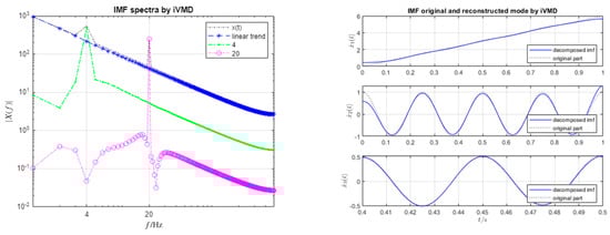
Figure 2. iVMD decomposition of $x_{\mathrm{Sig}1}\left(t\right)$. The left shows the IMF’s spectra, and the right shows the reconstructed modes. In the left figure, legend $x\left(t\right)$ expresses the spectrum of $x_{\mathrm{Sig}1}\left(t\right)$, and legend 4 and 20, respectively, express the spectra of the components at 4 Hz and 20 Hz.

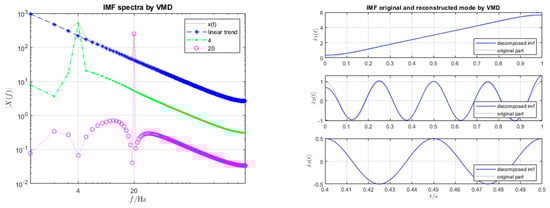
Figure 3. VMD decomposition of $x_{\mathrm{Sig}1}\left(t\right)$.

5.2. Example 2 with a Piecewise Signal

The second signal is

$$x_{\mathrm{Sig}2}\left(t\right)=6t^2+\cos \left(10\pi t+10\pi t^2\right)+\{\begin{array}{cc}\cos 60\pi t& t\le 0.5\\ \cos \left(80\pi t-10\pi \right)& t>0.5\end{array}$$

(42)

We set $K=4$ in the iVMD algorithm, thus assigning each half of the piecewise-constant frequency signal to a separate mode. Both iVMD and VMD achieve effective convergence with the expected center frequencies after carefully tuning the parameters of the respective algorithms. For details, see Figure 4 and Figure 5. When comparing the peaks in frequencies at 30, 40 Hz, the results run via iVMD show slightly better results.

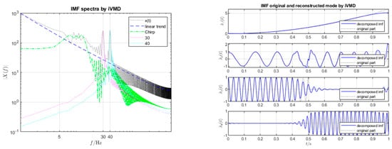
Figure 4. iVMD decomposition of $x_{\mathrm{Sig}2}\left(t\right)$ run via iVMD. The left figure shows the IMF’s spectra, and the right shows the reconstructed modes.

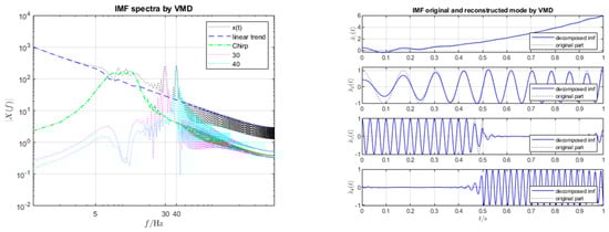
Figure 5. VMD decomposition of $x_{\mathrm{Sig}2}\left(t\right)$.

5.3. Example 3: Intrawave Frequency Modulation

The third signal is

$$x_{\text{Sig}3}\left(t\right)=\frac{1}{1.2+\cos \left(2\pi t\right)}+\frac{\cos \left(32\pi t+0.2\cos \left(64\pi t\right)\right)}{1.5+\sin \left(2\pi t\right)}$$

(43)

The iVMD and VMD results are almost identical, as illustrated in Figure 6 and Figure 7. In fact, the second term in (43) quickly converges with the correct main frequency of 16 Hz.

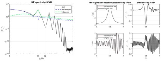
Figure 6. iVMD decomposition of $x_{\mathrm{Sig}3}\left(t\right)$ run via iVMD. The left shows the IMF’s spectra, and the right shows the reconstructed modes. In the reconstructed modes, we show four figures. The left two are the IMFs, and the right two show the differences between the estimated IMF and the original.

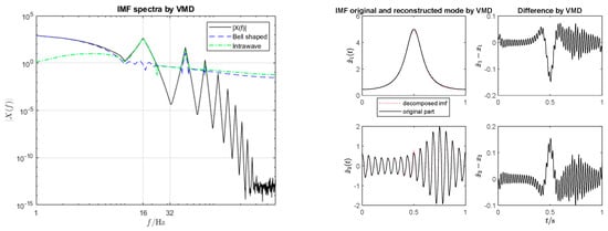
Figure 7. VMD decomposition of $x_{\mathrm{Sig}3}\left(t\right)$.

5.4. Example 4: Sawtooth Signal

The fourth signal is

$$x_{\mathrm{Sig}4}\left(t\right)=x_{41}\left(t\right)+x_{42}\left(t\right).$$

(44)

The components $x_{41},x_{42}$ are sawtooth signals of different center frequencies, 10 Hz and 80 Hz, and amplitudes at 2. Figure 8, run via iVMD, shows the decomposition of the two sawtooth composite signals. The iVMD algorithm can obtain effective decomposition with the relatively small-value difference curve between the raw sawtooth and the estimated sawtooth. The two are compared by running at different settings of harmonical order—$M$, $M=\left[1;3;5\right]$—the bigger $M$ is taken to allow more harmonical components, and the difference is smaller.

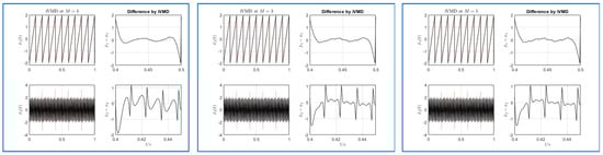
Figure 8. iVMD decomposition of $x_{\mathrm{S}\mathrm{i}\mathrm{g}4}\left(t\right)$ run via iVMD. The algorithm iVMD is run at $M=\left[1;3;5\right]$, the figures of which are noted in the titles. Each figure has four sub-figures, with the left two being decomposed IMFs and the originals, while the right two are the correspondence differences.

For comparison, we still provide the results run by the VMD with the same aspect, which is depicted in Figure 9. The difference between the original and decomposed signal is relatively smoother in the iVMD results.

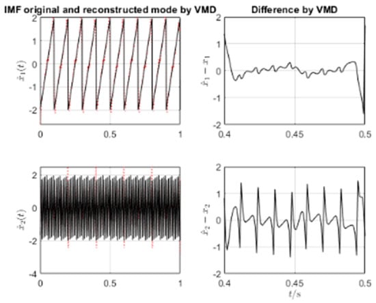
Figure 9. VMD decomposition of $x_{\mathrm{Sig}4}\left(t\right)$.

5.5. Example 5: An Electrocardiogram

The fifth signal, $x_{\mathrm{Sig}5}\left(t\right)$, is an electrocardiogram (ECG). The data are shared by [2]. The data present numerous components in which there exists an oscillating low-frequency pattern, and a noise with a high frequency. Figure 10 illustrates the spectra and the results run via iVMD. A high number of 12 modes is detected. The center frequencies are effectively detected, which converges with ECG spectral peaks. The first mode represents the baseline oscillation, and the last mode represents the high-frequency noise.

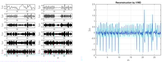
Figure 10. iVMD decomposition of $x_{\text{Sig}5}\left(t\right)$. We set $K=12$. The left figure shows the IMFs, and the right shows the reconstructed ECG signal, where the first and last modes are discarded.

6. Conclusions and Outlook

We further developed the algorithm of VMD as iVMD from three points: (1) flattest response, (2) harmonic, and (3) bandwidth. The flattest response is applied in iVMD and thus, we can set the higher differential order $P$ with respect to time, which results in the added weighting coefficient which can be obtained via Butterworth filter designing. As the harmonics may exist in the input signal, the mathematical model of VMD is further studied and modified via the harmonic order $M$, and the improved version can support $M$-order harmonical center frequency, $m{\omega }_k$. Each mode may have its adaptive bandwidth, and we set it in the model in (13) and (17). Through the above three points, we developed the algorithm iVMD.

In our experiments, iVMD works effectively with the same abilities as VMD and achieves a better performance than VMD.

The assumption of iVMD is the same as VMD, except that we can set the differential order and harmonic order with adjustable bandwidth, $B_k$. We explain the reasons behind decomposing the two sawtooth composite signals, and it is due to setting the M-order harmonics in the mathematical model.

The algorithm iVMD is now being further extended with two-dimension decomposition, and we expect further challenges to decompose more complex composite signals.

References

- Crochiere, R. A weighted overlap-add method of short-time Fourier analysis/synthesis. IEEE Trans. Acoust. Speech Signal Process. 1980, 28, 99–102. [Google Scholar] [CrossRef]
- Gilles, J. Empirical wavelet transform. IEEE Trans. Signal Process. 2013, 61, 3999–4010. [Google Scholar] [CrossRef]
- Liu, S.; Yu, K. Successive multivariate variational mode decomposition based on instantaneous linear mixing model. Signal Process. 2022, 190, 108311. [Google Scholar] [CrossRef]
- Huang, N.E.; Shen, Z.; Long, S.R.; Wu, M.C.; Shih, H.H.; Zheng, Q.; Yen, N.C.; Tung, C.C.; Liu, H.H. The empirical mode decomposition and the Hilbert spectrum for nonlinear and non-stationary time series analysis. Proc. R. Soc. London. Ser. A Math. Phys. Eng. Sci. 1998, 454, 903–995. [Google Scholar] [CrossRef]
- Dragomiretskiy, K.; Zosso, D. Variational Mode Decomposition. IEEE Trans. Signal Process. 2014, 62, 14. [Google Scholar] [CrossRef]
- Chen, S.; Dong, X.; Peng, Z.; Zhang, W.; Meng, G. Nonlinear chirp mode decomposition: A variational method. IEEE Trans. Signal Process. 2017, 65, 6024–6037. [Google Scholar] [CrossRef]
- Deb, S.; Dandapat, S.; Krajewski, J. Analysis and classification of cold speech using variational mode decomposition. IEEE Trans. Affect. Comput. 2020, 11, 296–307. [Google Scholar] [CrossRef]
- Nazari, M.; Sakhaei, S.M. Successive variational mode decomposition. Signal Process. 2020, 174, 107610. [Google Scholar] [CrossRef]
- Chen, S.; Yang, Y.; Peng, Z.; Dong, X.; Zhang, W.; Meng, G. Adaptive chirp mode pursuit: Algorithm and applications. Mech. Syst. Signal Process. 2019, 116, 566–584. [Google Scholar] [CrossRef]
- Dragomiretskiy, K.; Zosso, D. Two-Dimensional Variational Mode Decomposition. In Energy Minimization Methods in Computer Vision and Pattern Recognition; Springer: Cham, Switzerland, 2015. [Google Scholar]
- Zosso, D.; Dragomiretskiy, K.; Bertozzi, A.L.; Weiss, P.S. Two-Dimensional Compact Variational Mode Decomposition. J. Math. Imaging Vis. 2017, 58, 294–320. [Google Scholar] [CrossRef]
- Ur Rehman, N.; Aftab, H. Multivariate variational mode decomposition. IEEE Trans. Signal Process. 2019, 67, 6039–6052. [Google Scholar] [CrossRef]
- Chen, Q.; Lang, X.; Xie, L.; Su, H. Multivariate intrinsic chirp mode decomposition. Signal Process. 2021, 183, 108009. [Google Scholar] [CrossRef]
- Stanković, L.; Brajović, M.; Daković, M.; Mandic, D. On the decomposition of multichannel nonstationary multicomponent signals. Signal Process. 2020, 167, 107261. [Google Scholar] [CrossRef]
- Liu, W.; Hu, W.; Fu, D. Frequency Shifting-based Variational Mode Decomposition Method for Speech Signal Decomposition [Z]. In Proceedings of the 2022 International Conference on Automation, Robotics and Computer Engineering (ICARCE), Wuhan, China, 16–17 December 2022. [Google Scholar]
- Dendukuri, L.S.; Hussain, S.J. Emotional speech analysis and classification using variational mode decomposition. Int. J. Speech Technol. 2022, 25, 457–469. [Google Scholar] [CrossRef]
- Bagheri, A.; Ozbulut, O.E.; Harris, D.K. Structural system identification based on variational mode decomposition. J. Sound Vib. 2018, 417, 182–197. [Google Scholar] [CrossRef]
- Chang, L.; Wang, R.; Zhang, Y. Decoding SSVEP patterns from EEG via multivariate variational mode decomposition-informed canonical correlation analysis. Biomed. Signal Process. Control. 2022, 71, 103209. [Google Scholar] [CrossRef]
- Li, G.; Tang, G.; Luo, G.; Wang, H. Underdetermined blind separation of bearing faults in hyperplane space with variational mode decomposition. Mech. Syst. Signal Process. 2019, 120, 83–97. [Google Scholar] [CrossRef]
- Zhang, X.; Chen, Y.; Jia, R.; Lu, X. Two-dimensional variational mode decomposition for seismic record denoising. J. Geophys. Eng. 2022, 19, 433–444. [Google Scholar] [CrossRef]
- Guo, Y.; Zhang, Z. Generalized Variational Mode Decomposition: A Multiscale and Fixed-Frequency Decomposition Algorithm. IEEE Trans. Instrum. Meas. 2021, 70, 1–13. [Google Scholar] [CrossRef]
- Rockafellar, R.T. A dual approach to solving nonlinear programming problems by unconstrained optimization. Math. Program. 1973, 5, 354–373. [Google Scholar] [CrossRef]
- Bertero, M.; Poggio, T.A.; Torre, V. Ill-posed problems in early vision. Proc. IEEE 1988, 76, 869–889. [Google Scholar] [CrossRef]
- Morozov, V.A. Linear and nonlinear ill-posed problems. J. Math. Sci. 1975, 2, 706–736. [Google Scholar] [CrossRef]
- Butterworth, S. On the theory of filter amplifires. Exp. Wirel. 1930, 7, 536–541. [Google Scholar]
- Bertsekas, D.P. Multiplier methods: A. survey. Automatica 1976, 12, 133–145. [Google Scholar] [CrossRef]
- Bertsekas, D.P. Constrained Optimization and Lagrange Multiplier Methods; Academic Press: Boston, MS, USA, 1982. [Google Scholar]
- Oppenheim, A.V.; Schafer, R.W.; Buck, J.R. Discrete-Time Digital Signal Processing; Prentice Hall, Inc.: Hoboken, NJ, USA, 1998. [Google Scholar]
Disclaimer/Publisher’s Note: The statements, opinions and data contained in all publications are solely those of the individual author(s) and contributor(s) and not of MDPI and/or the editor(s). MDPI and/or the editor(s) disclaim responsibility for any injury to people or property resulting from any ideas, methods, instructions or products referred to in the content. |
© 2023 by the authors. Licensee MDPI, Basel, Switzerland. This article is an open access article distributed under the terms and conditions of the Creative Commons Attribution (CC BY) license (https://creativecommons.org/licenses/by/4.0/).