Article

Model for Choosing the Shape Parameter in the Multiquadratic Radial Basis Function Interpolation of an Arbitrary Sine Wave and Its Application

College of Science, North China University of Science and Technology, Tangshan 063210, China
*
Authors to whom correspondence should be addressed.
Mathematics 2023, 11(8), 1856; https://doi.org/10.3390/math11081856
Submission received: 17 March 2023 / Revised: 10 April 2023 / Accepted: 11 April 2023 / Published: 13 April 2023
(This article belongs to the Special Issue Novel Mathematical Methods in Signal Processing and Its Applications)

Abstract

:
In multiquadratic radial basis function (MQ-RBF) interpolation, shape parameters have a direct effect on the interpolation accuracy. The paper presents an MQ-RBF interpolation technique with optimized shape parameters for estimating the parameters of sine wave signals. At first, we assessed the impact of basic sinusoidal parameters on the MQ-RBF interpolation outcomes through numerical experiments. The results indicated that the angular frequency of a sine wave is a crucial determinant of the corresponding MQ-RBF interpolation shape parameters. A linear regression method was then used to establish the optimal parameter selection formula for a single-frequency sine wave, based on a large volume of experimental data. For multi-frequency sinusoidal signals, appropriate interpolation shape parameters were selected using the random walk algorithm to create datasets. These datasets were subsequently used to train several regression models, which were then evaluated and compared. Based on its operational cost and prediction accuracy, the random forest algorithm was chosen to establish the shape parameter selection model for multi-frequency sinusoidal signals. The inclusion of the Bayesian optimizer resulted in a highly accurate model. The establishment of this model enabled the adaptive selection of the corresponding shape parameters for any sine wave signal, providing a convenient means of selecting MQ-RBF interpolation shape parameters. Furthermore, the paper proposes an MQ-RBF interpolation subdivision least squares method that significantly improves the estimation accuracy of sine wave parameters. The practicality of the method was validated by successfully applying it in the calibration of the clock delay mismatch of a time-interleaved analog-to-digital converter system.

1. Introduction

Interpolating a set of ordered data points is the process of constructing a curve that passes through these points. The quality of the interpolation results is directly impacted by the selected interpolation basis function. According to Frank [1], among the 29 interpolation methods tested using different datasets, the MQ-RBF interpolation method yielded the highest accuracy. Numerous studies have demonstrated that the shape parameters of the MQ-RBF significantly affect the interpolation accuracy [2,3,4]. Sinusoidal phenomena, including vibration, swing, and fluctuation, are common in natural systems. Sinusoidal waves can be applied in various technologies, such as frequency, amplitude, and phase modulation in radio, television, communication, and navigation. In signal processing, the estimation of sine parameters [5] is highly significant and useful, since numerous problems can be simplified to sine problems. Currently, there is no comprehensive or efficient technique to determine the appropriate shape parameters of the MQ-RBF for a specified sine wave. Therefore, establishing an MQ-RBF interpolation shape parameter selection model for sine waves has significant scientific and practical significance.
In engineering design, curves are often necessary to approximate a series of real objects that meet certain requirements. These ordered data points may contain errors due to various factors, and the curves or surfaces reflecting the experimental data do not necessarily need to pass through each point. Hence, a fitting method is used to approximate these discrete points, with the least squares fitting method [6] being the most commonly used approach. However, sometimes, it is necessary to use original data points as much as possible, and the accuracy of the fitting calculation also needs to be high, at which point the least squares method alone cannot meet these requirements. To address this problem, we proposed a method of least squares sine curve fitting by increasing the data volume through MQ-RBF interpolation. In this method, we adaptively selected shape parameters for interpolation through the shape parameter selection model for sine waves, which is constructed in this paper. From there, we obtained refined values according to the processing requirements. Finally, we fit the refined values using least squares and determined the sine wave parameters.
As digital signal processing speed continues to improve, modern communication and radar systems require increasingly faster analog-to-digital conversion speeds. A time-interleaved analog-to-digital converter (TIADC) system can effectively enhance the conversion speed. However, process and device aging can result in a mismatch in clock delay between adjacent channels, which distorts the output spectrum of the TIADC system and reduces system resolution. Therefore, correcting the clock delay mismatch is essential [7]. Two methods are used to calibrate TIADC system outputs [8,9,10,11]. The first method measures the error caused by the clock delay mismatch of the output points of each channel of the TIADC system through test signals, then uses this error to calibrate the output sampling points of the TIADC system. In contrast, the second method estimates the clock delay of each channel first, then uses digital signal processing on the output data to calibrate the system output. These methods have their own advantages and disadvantages: the former does not require the measurement of the clock delay of each channel but takes hours to generate the error table, while the latter has a shorter runtime but relies on the algorithm’s convergence and accuracy. Consequently, accurately estimating the clock delay is essential for the latter calibration method. In this paper, we propose a model-based method to obtain an effective sinusoidal signal in the TIADC system output signal by applying our proposed method to the multi-frequency sinusoidal fitting of the output data. We then used the relationship between the system’s output spectrum and the effective sinusoidal signal to determine the clock delay of each channel. Finally, to verify the effectiveness of this approach, we conducted experimental simulations.

2. Selection of Shape Parameters in MQ-RBF Interpolation

2.1. MQ-RBF

MQ-RBF [12,13,14] is a radial basis function expressed as:
f k ( x ) = ( | | x - x k | | ) 2 + c 2
where c is a shape parameter and the nodes x k k = 1 , 2 , N are distinct. MQ-RBF interpolation, defined as [15], MQ-RBF ϕ : R + R is used to obtain an interpolation function with shape s x = k = 1 N ω k ϕ x x k ( ω k is interpolation coefficient) to conform to conditions s x k = f k , k = 1 , 2 , N , given a specific set of sample data x k , f k k = 1 N R n R .

2.2. MQ-RBF Shape Parameters Chosen Using the Random Walk Algorithm

The following optimization problem can be used to represent the MQ-RBF shape parameter selection:
E max c = max x a , b | s x , c f x |
F i n d   c o p t min E max c s . t .   i < 1000 , θ < 10 8 , ε < 10 9 c > 0
These parameters include the interpolation basis function s x , c , the interpolation primitive function f x , the maximum error E max c , the required optimal shape parameter c o p t , the number of walks i , the step control accuracy θ , and the error control accuracy ε .
The shape parameters of the MQ-RBF interpolation are selected through the random walk algorithm, a global optimization technique [16]. The results of this algorithm selection have been shown to significantly improve interpolation accuracy. Figure 1 presents a flowchart of this algorithm.
The algorithm to select optimal shape parameters ( c o p t ) follows these steps:
  • Step 1: Specify i i = 1 , 2 , M as the number of walks, k k = 1 , 2 , N as the number of current iterations, accuracy θ for step control, and accuracy ε for error control. Set k = 1 and the initial parameter c 0 .
  • Step 2: The initial step length is λ 0 for the first walk. Each iteration generates a random N-dimensional vector u i k = ( u 1 , , u j , , u n ) , u i k ( q , q ) , which is then standardized to obtain u i k = u i k j = 1 n u j 2 , satisfying c 1 = c 0 + λ 0 u 1 k , , c i = c i 1 + λ u i k .
  • Step 3: Calculate the value of E max c i :
(1) If condition E max c i < E max c i 1 holds, it indicates that the i th step has been successfully completed. Subsequently, we take parameter c i as a new initial value, initiate a reset of parameter k to 1, and commence the subsequent walk. We repeat the walk process until either E max c < ε or i = M is met. This marks the termination of the algorithm.
(2) If condition E max c i > E max c i 1 holds, it indicates that the current parameter has not been improved. In the event that k < N holds, the algorithm returns to step 2 to generate new random vectors ( u i k + 1 , u i k + 2 , , u i N 1 ) and continue the search. Conversely, in the condition that no better parameter is discovered ( k = N ), the optimal parameter ( c o p t ) is deemed to be within a sphere with center ( c i 1 ) and a radius ( λ ). If λ < θ is met, the algorithm is terminated; otherwise, the value of λ = λ 0 / 2 is set, and the algorithm reverts back to step 1 to initiate a new cycle of the search.

3. MQ-RBF Interpolation of Sine Waves

3.1. Basic Parameters of Sine Waves

The sine function is paramount in the fields of mathematics and engineering. When dynamic concepts such as amplitude, angular frequency, phase, and offset are incorporated, the sine function transforms from a fixed value to a wave. This wave is commonly referred to as a sine wave or a sine curve in signal processing and can be expressed mathematically as follows [17]:
y = A sin ω t + φ + B
where A corresponds to the amplitude of the wave. If an object undergoes linear reciprocating motion with a trajectory conforming to a sine wave, A equals half the stroke. ω t + φ represents the phase and reflects the state of the variable y , and φ indicates the initial phase of t = 0 . In practical applications, B denotes the offset and becomes unified with the DC component (the amplitude of a wave with a frequency of 0). ω represents the angular frequency, i.e., the number of vibrations per unit radian, and thereby controls the period of the sine wave.
T = 2 π / ω

3.2. Influence of Sine Wave Basic Parameters on MQ-RBF Interpolation

In this section, four numerical experiments are illustrated to explore the effects of the sine wave characteristics on MQ-RBF interpolation, represented by four parameters labeled φ , B , A and ω . To fit the overall function and consider practical problems, we used one period of the sine wave as the interval length of the independent variable value in these experiments.
The MQ-RBF interpolates Function (6) by applying the algorithm flow outlined in Section 2.2. The results are presented in Table 1, while Figure 2 showcases the interpolation effect and the absolute error image of Function (6). The shape parameters selected by the algorithm delivered a well-fitted effect.
y = sin π x
  • Experiment 1: Changing φ .
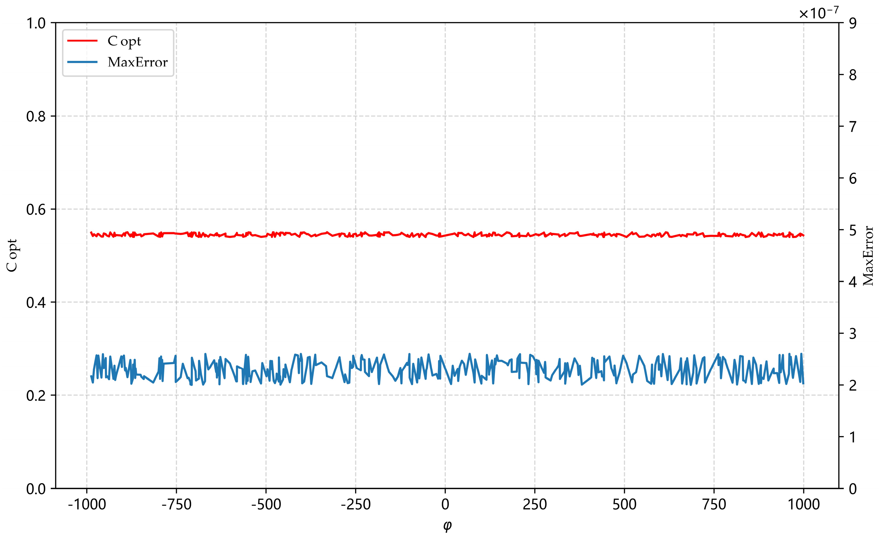
We arbitrarily transformed φ in Function (7). The function was interpolated by the MQ radial basis function, and its corresponding parameters were determined by our algorithm; then, this process was repeated. Some experimental results are shown in Table 2. Figure 3 shows the changes in c o p t and M a x E r r o r with the change in φ . From the figure, it can be seen that almost all points were concentrated on the same horizontal line, so φ had little influence on the interpolation results.
y = s i n π x + φ
  • Experiment 2: Changing B .
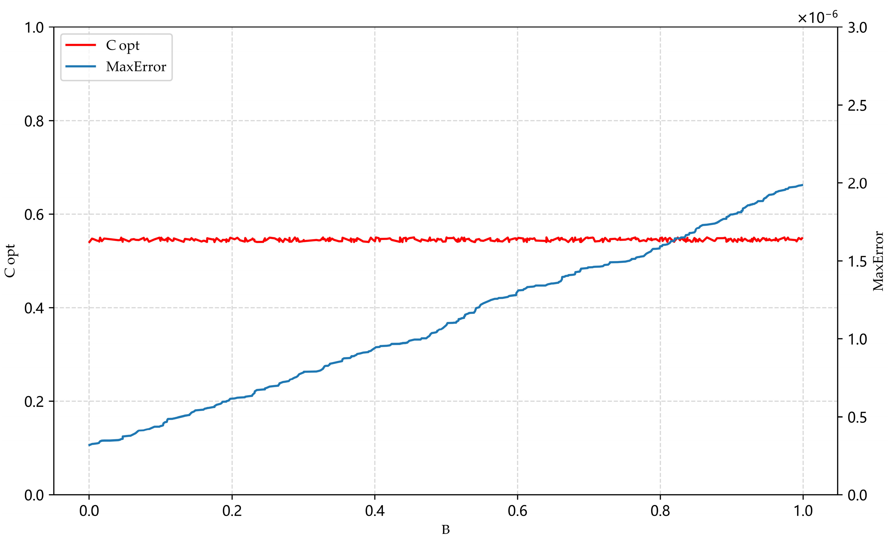
Function (6) was used to carry out MQ-RBF interpolation after adding B (Function (8)). The relationship between B and c o p t , M a x E r r o r , is shown in Figure 4.
y = s i n π x + B
According to Figure 4, based on the interpolation error of Experiment 1, with the increase in B , the corresponding c o p t still had no obvious change, but the M a x E r r o r continued to increase. In the practical application of sine waves, B is also called “noise data”, so making B as small as possible can improve the interpolation accuracy.
  • Experiment 3: Changing A .
    y = A s i n π x
For A 10 , 10 , different A and corresponding c o p t and M a x E r r o r values were determined by our algorithm. Some experimental results are shown in Table 3.
According to Table 3, with the change in A , c o p t had no obvious change, but the corresponding change in M a x E r r o r was substantial. In order to explore the influence of A on interpolation accuracy, the amplitude range was amplified or reduced by 10 times, i.e., A 100 , 100 or A 1 , 1 . Some experimental data are presented in Table 4.
According to the experimental results, the interpolation error accuracy decreased or increased by approximately one order of magnitude when the range of A was expanded or contracted by a factor of 10. To ensure the correctness of the error analysis, we further compared and verified the interpolation accuracy when expanding or reducing the range by 100 times. Table 5 presents some experimental findings.
The verification indicated that the aforementioned conclusion was still true. According to Table 3, Table 4 and Table 5, the value of A had a significant impact on the interpolation error accuracy but minimal impact on the value of the shape parameters. The M a x E r r o r changed proportionately with A .
  • Experiment 4: Changing ω .
In order to explore the relationship between c o p t and T , the ω of Function (10) was changed.
y = sin ω x
Let ω = π / k , ω = k π k = 2 , , 10 , that is, compared with Function (6), T was expanded or reduced k times. Some experimental results are shown in Table 6 and Table 7.
In Table 6 and Table 7, the error results are basically consistent with those in Table 1 and Table 2, so the change in T had little influence on the interpolation accuracy. The T value was proportional to the c o p t value. We enlarged or reduced T by 10 k k = 1 , 2 , , 10 times to continue verification, and some experimental results are shown in Table 8 and Table 9.
From Table 8 and Table 9, c o p t still changed in correspondence with the change in T , which again verified the above conclusion.

3.3. Shape Parameter Selection Model for Single-Frequency Sine Wave and Its Verification

From the numerical experiments in Section 3.2, it can be seen that the T of a single-frequency sine wave is a factor that directly affects the c o p t , and they display a positive correlation. The c o p t of any single-frequency sine wave was selected by the RW algorithm, and the model (Equation (11)) was fitted by a linear regression method under a large amount of data. Figure 5 is a schematic diagram of the linear model.
c o p t = 0.272619 T + 0.1668
For any single-frequency sine wave (see Table 10 for some test functions), Formula (11) determines the shape parameters, which are then compared to results obtained directly by our algorithm (refer to Table 11). From the experimental findings, it can be deduced that the predicted shape parameters were precise.

4. Shape Parameter Selection Model for Multi-Frequency Sinusoidal Signal

4.1. Shape Parameter Selection for Multi-Frequency Sinusoidal Signal

A multi-frequency sinusoidal signal [18] refers to a periodic signal that represents the summation of various discrete frequency sinusoidal signals. Typically utilized to rapidly test the frequency properties of linear systems, the multi-frequency sine signal can be expressed mathematically as follows:
x t = k = 1 N A k cos ω k t + θ k
where N is the number of harmonics contained in the signal, and A k , ω k , θ k are the amplitude, angular frequency, and initial phase of the k t h harmonic, respectively. Through experiments, combined with the exploration of the single-frequency sine wave signal in Section 3.2, it was finally verified that the ω k of the multi-frequency sine wave signal was still a factor that directly affected the value of its shape parameters.
This section employs the random walk algorithm to select MQ-RBF interpolation shape parameters for one million mixed sinusoidal signals with varying frequencies to accumulate preliminary data. In this experiment, to fit all frequency characteristics of the signal, the independent variable values were taken from one period of the maximum period (the lowest angular frequency).
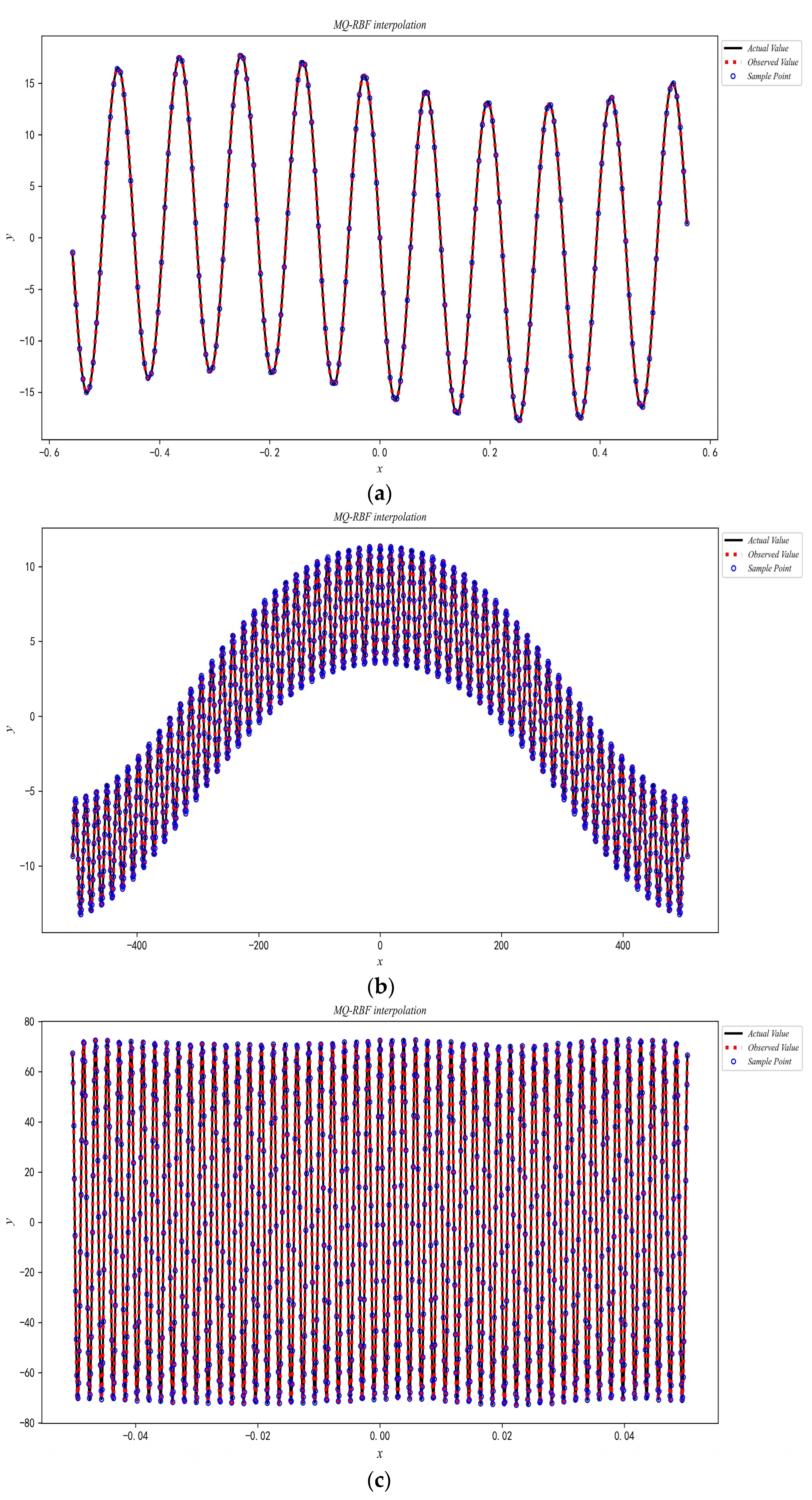
Several test findings and their corresponding MQ-RBF interpolation effect diagrams (refer to Figure 6) are presented below. It was apparent that the fitting effects of the form parameters determined in this study remained excellent, even when there was the superposition of numerous frequency signals.
  • Two-frequency superposition signal:
    y = 2.4516 s i n 1.7927 π x 15.3975 s i n 17.8744 π x c o p t = 0.03578 , M a x E r r o r = 4.87 × 10 5
  • Three-frequency superposition signal:
    y = 84.877 sin 0.00097 π x 1.0142 sin 0.00371 π x + 3.8966 sin 0.11562 π x c o p t = 4.6985 ,   M a x E r r o r = 1.55 × 10 4
  • Four-frequency superposition signal:
    y = 0.08092 sin 19.8758 π x + 0.9401 sin 46.6415 π x + 0.4338 cos 67.435 π x + 71.5436 sin 1031.146 π x   c o p t = 0.000142 ,   M a x E r r o r = 6.69 × 10 4
  • Five-frequency superposition signal:
    y = 571.54 sin 0.00000424 π x + 11.6523 sin 0.000098 π x + 204.79 sin 0.000056 π x 1.121 sin 0.000092 π x 57.2577 sin 0.00011 π x   c o p t = 4258.002 ,   M a x E r r o r = 1.80 × 10 4
  • Six-frequency superposition signal:
    y = 9.4471 s i n 0.00058 π x + 0.8724 s i n 0.00136 π x + 3.8422 c o s 0.01027 π x 0.46931 s i n 0.00453 π x 0.14899 s i n 0.14761 π x 0.4148 c o s 0.02485 π x c o p t = 14.3633 , M a x E r r o r = 1.20 × 10 4

4.2. Selection of Regression Model

Over one million multi-frequency sinusoidal signals and their corresponding shape parameters were segmented using the Pandas library in Python 3.10. Of these, 900,000 pieces of data were chosen to form the training sets. Subsequently, the random forest (RF), multiple linear regression (MLR), gated recurrent unit (GRU) networks, support vector machine (SVM), and long short-term memory (LSTM) models were trained using the aforementioned sets [19,20,21,22,23]. The remaining 100,000 pieces of data were used to form the test set and to compare and evaluate the effectiveness of the different models (refer to Table 12). The evaluation indices primarily included training time, goodness of fit ( R 2 ), mean square error (MSE), and mean absolute error (MAE).
Our experimental observations revealed that MLR had the poorest prediction accuracy despite the shorter training time. This inadequacy could have resulted from a lack of a clear linear relationship between the data. SVM exhibited limitations in managing large-scale samples, with an average training time and prediction accuracy. On the other hand, with a comparable training time, the random forest model had the highest accuracy in predicting the shape parameters of multi-frequency sinusoidal signals compared to GRU and LSTM. After a thorough comparison, we opted for the random forest model to undertake shape parameter prediction.

4.3. Bayesian Optimization-Based Random Forest Method to Construct Shape Parameter Selection Model

Random forest (RF) [19] is an efficient ensemble learning algorithm grounded in classification trees. It generates multiple independent decision trees by randomly selecting training samples and feature subgroups, after which it consolidates the output of these decision trees. In order to predict a new input, each decision tree is traversed, and the final averaged results of all trees bestow the model with more dependable prediction capabilities.
Among the parameters of RF, n _ e s t i m a t o r s is the number of decision trees, and too few decision trees easily lead to under-fitting. The more decision trees, the better the algorithm effect, but the calculation time also increases. When the number of trees exceeds a critical value, the effect of the algorithm is not significantly improved. M a x _ f e a t u r e s is the maximum number of features, that is, the maximum number of features considered when constructing the optimal model of the decision tree. The lower this value, the more the variance decreases, but the more the deviation increases. M i n _ s a m p l e s split is the minimum number of samples that can be divided into nodes, and M a x _ d e p t h is the maximum depth of the decision tree. We needed to optimize the parameters of RF in order to obtain the best parameters.
The optimization of machine learning hyperparameters can be carried out using a range of techniques, including grid search, random search, and Bayesian optimization. Bayesian optimization [24] is commonly utilized in parameter combination optimization since it can produce superior results with fewer iterations than grid search or random search and rapidly identify the best solution for hyperparameters.
The Bayesian optimization–random forest (BO-RF) algorithm confers several benefits [25]. It is fast in processing; effective in handling large-scale datasets, such as those used in this research; and robust to noise in datasets. In contrast to the conventional machine learning approach, BO-RF is more practical in dealing with nonlinear data. It does not encounter the multicollinearity problem that ordinary regression analysis faces. The algorithm is suitable for high-dimensional feature vector space, with the benefits of a high prediction accuracy, fast convergence rate, fewer modification parameters, and the efficient avoidance of “over-fitting”.
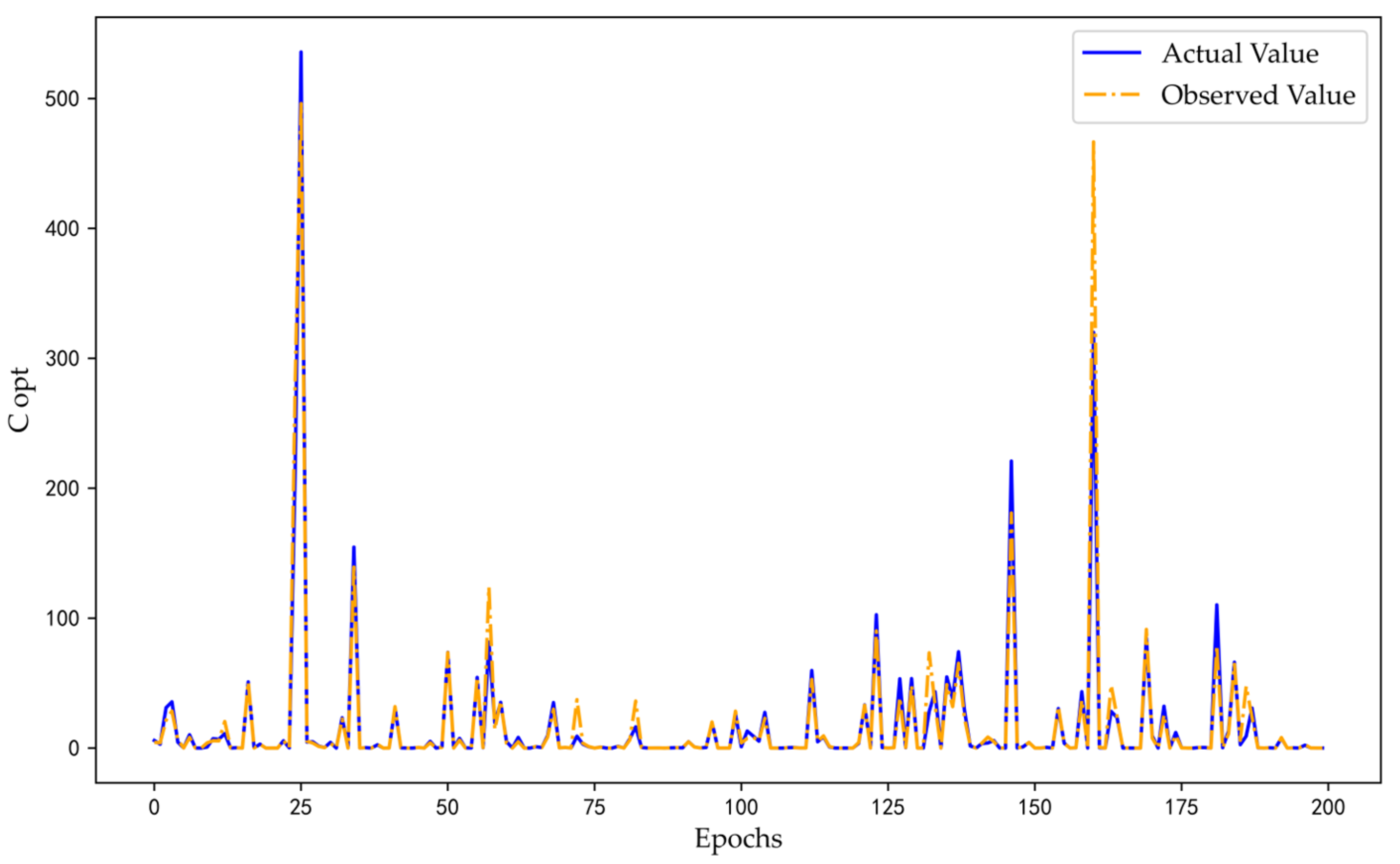
The optimization of model parameters was carried out through Bayesian optimization, while the model was trained using the five-fold cross-validation technique. The model was fed with 589 decision trees, ensuring a maximum feature number of 0.703, a minimum sample size of 1, a maximum depth of 84, a molecular radius of 1.0, and a molecular fingerprint length of 128. Subsequently, the effectiveness of the model was tested using the test set, and Table 13 shows the results of the tests. Without significantly increasing the computational time, the model significantly reduced its MSE, MAE and R 2 values. The results indicated that the model possessed good generalization and resilience capabilities as well as a high prediction accuracy. Furthermore, Figure 7 illustrates a line chart that compares the predicted values with the actual values of some of the data. The chart demonstrates that the fluctuations in the predicted values and the actual values were virtually identical, indicating that the model’s fitting accuracy was good.

5. Application of Model

5.1. MQ-RBF Interpolation Subdivision Least Squares Method

5.1.1. Parameter Estimation of Sine Signal

In signal processing, the estimation of sine parameters is highly significant and useful, since numerous problems can be simplified to sine problems. Four critical parameters determine a sine wave’s mathematical uniqueness, namely the amplitude, angular frequency, phase, and DC offset. The estimation of sine parameters aims to determine these factors accurately. Equation (18) is primarily utilized in sine fitting applications.
y t = A 1 sin 2 π f t + A 2 cos 2 π f t + B       = A sin 2 π f t + φ + B
The data recording sequence is a sample y 1 , y 2 , y n at the moment t 1 , t 2 , t n . In the actual signal problem, the signal sampling is usually uniform. When the rate v is known, the sampling interval is Δ t , t k = k × Δ t = k / v , k = 1 , 2 , n , and the angular frequency is ω = 2 π f / v , the formula can be changed into the following discrete form:
y k = A 1 sin ω k + A 2 cos ω k + B
Therefore, a uniformly sampled sine wave can be uniquely represented by A 1 , A 2 , B and k. This is analogous to knowing the angular frequency of the sampling to be able to determine the position of each sampling value in the experiment. Many studies have demonstrated that three-parameter sine wave curve fitting with regard to amplitude, phase, and DC offset is a closed linear process for a given frequency [26]. The results may be produced without iteration, and there is no convergence problem; therefore, it has strong practicability.

5.1.2. MQ-RBF Interpolation Subdivision Least Squares Method for Fitting a Sine Signal

Sine wave parameters can be obtained using the least squares method (LS) [27], but in some circumstances it may be necessary to employ as many known data points as feasible. The needs of data processing cannot currently be met by LS alone. The interpolation approach uses the value of the function at a small number of locations to estimate the function’s approximate value at other places. This study developed the MQ-RBF interpolation subdivision–least squares (MQ-LS) fitting method for sine waves based on the foregoing details. The technique included the following detailed steps:
  • Step 1: We selected appropriate interpolation shape parameters for known frequencies using the model.
  • Step 2: Based on this shape parameter, MQ-RBF was used to interpolate between the sampled data to increase the data volume.
  • Step 3: Following interpolation and refinement, the data were fitted using least squares, and the outcomes were validated.
Simulated experiments were run in the following three groups. Table 14 lists three practical signal problems’ sample counts and theoretical sine wave expressions. The MQ-LS method (Table 15) was contrasted with the parameters that LS (Table 16) directly fitted.
From Table 15 and Table 16, it can be concluded that the MQ-LS method had smaller absolute errors and was closer to the real parameter values compared to the results obtained through direct fitting using the LS method. Notably, the estimation accuracy of the φ in all three groups of experiments was greatly improved. These findings demonstrated the effectiveness and practicality of the method employed.

5.2. Application of Model in Channel Clock Delay Problem of TIADC System

5.2.1. Multi-Frequency Sine Fitting and Output Signal of TIADC System

Multi-frequency sine fitting evolved from the single-frequency sine fitting algorithm and is used to obtain the fitting expression of p sine signals in discrete signals. Each sine signal in a discrete signal can be expressed as:
y l n = A l cos ω l n + B l cos ω l n + C l , n = 0 , , N 1
where C l is a DC component, and l = 0 , 1 , , p 1 . A l , B l , C l , ω l are unknown parameters to be solved. ω l = 2 π f l / f s , f l is the signal frequency, and the sampling rate is f s . The discrete signal output y n by the system is the sum of p sine signals and additional noise components e n , namely:
y n = l = 0 p 1 y l n + e n , n = 0 , , N 1
The noise e n is Gaussian white noise with a mean value of 0 and a variance of σ 2 .
Time-interleaved analog-to-digital converter (TIADC) systems can greatly increase the speed of analog-to-digital conversion. The output signal of a TIADC system is a combination of discrete signals, which can be expressed as follows:
y n = l = 0 M p 1 s l n
Due to the quantization error of each channel of the sampling system and the distortion of clutter, Equation (22) can be transformed into:
y n = l = 0 M p 1 y l n + e l n = l = 0 M p 1 y l n + e n
By comparing Equations (21) and (23), it is evident that the output of a TIADC system is equivalent to the multi-frequency sine fitting model. Therefore, the sine signal in the output of the TIADC system can be obtained using the multi-frequency sine fitting method.

5.2.2. Channel Clock Delay in TIADC System

Clock delay mismatch between adjacent channels in a TIADC system can occur due to processing, device aging, and other factors. For the input signal x t , when there is no clock delay mismatch between M channels of the T I A D C system, if the sampling period of the system is T s and the delay between two adjacent channels is equal to T s , the discrete sequence of the output of the i t h channel of the system can be expressed as:
u i n = x k M T s + i T s
If the delay between two adjacent channels deviates from T s , there is clock delay mismatch in the system, and the discrete sequence of the output of the i t h channel of the system is:
u i n = x k M T s + i T s Δ i
where Δ i shows the deviation of the actual sampling time of the channel from the ideal sampling time. Clock delay mismatch leads to the distortion of the output spectrum of the TIADC system and reduces the resolution of the system. Therefore, the clock delay mismatch must be calibrated.
The primary calibration techniques for TIADC systems involve estimating the clock delay of each channel and processing the output data with a digital signal. While this technique is efficient, the accuracy and convergence of the clock delay estimation algorithm have a significant impact on its effectiveness. Therefore, precise clock delay estimation is crucial. The clock delay of each channel can be determined by obtaining the amplitude and phase of the sine signal associated with each frequency, based on the characteristics of the TIADC system’s output spectrum and its relationship with the multi-frequency sine signal expression. For this research, the following calibration techniques were employed.
Firstly, the model-based selection of shape parameters was performed using the sampling data. Next, unknown sine parameters were fitted using the MQ-RBF interpolation subdivision–least squares method. Subsequently, the channel clock delay was calculated based on these parameters, and the system output was calibrated accordingly. Finally, the signal-to-noise-distortion ratio (SINAD) [28] of the system was compared before and after calibration to demonstrate the effectiveness of the algorithm, with improved SINAD serving as proof of its efficacy. The reduced channel clock delay mismatch resulting from improved SINAD further confirmed the viability of the proposed approach. Equation (26) was used to compute the system SINAD.
S I N A D = y 2 n / y n y n 2
where y n is the ideal output without channel mismatch, and y n is the actual output.
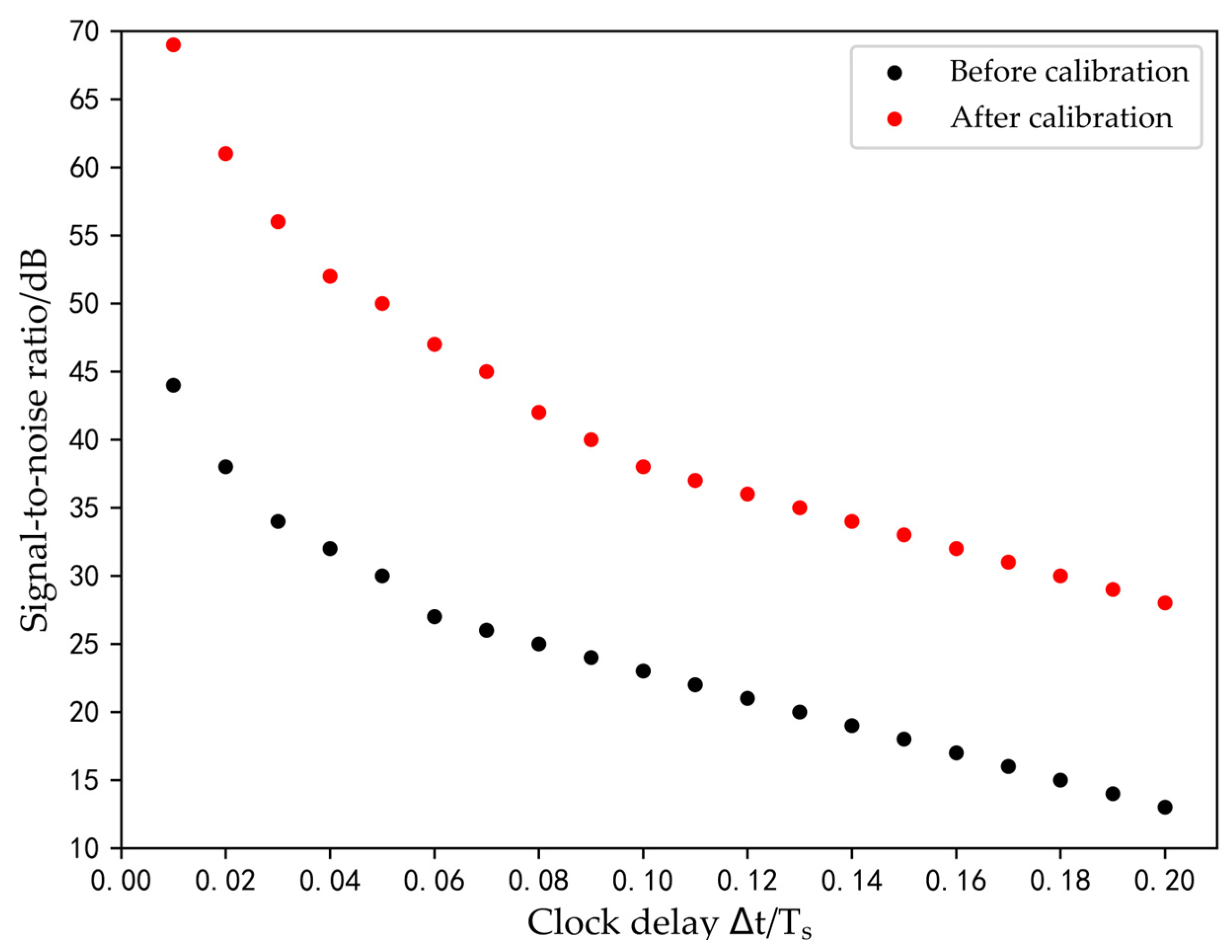
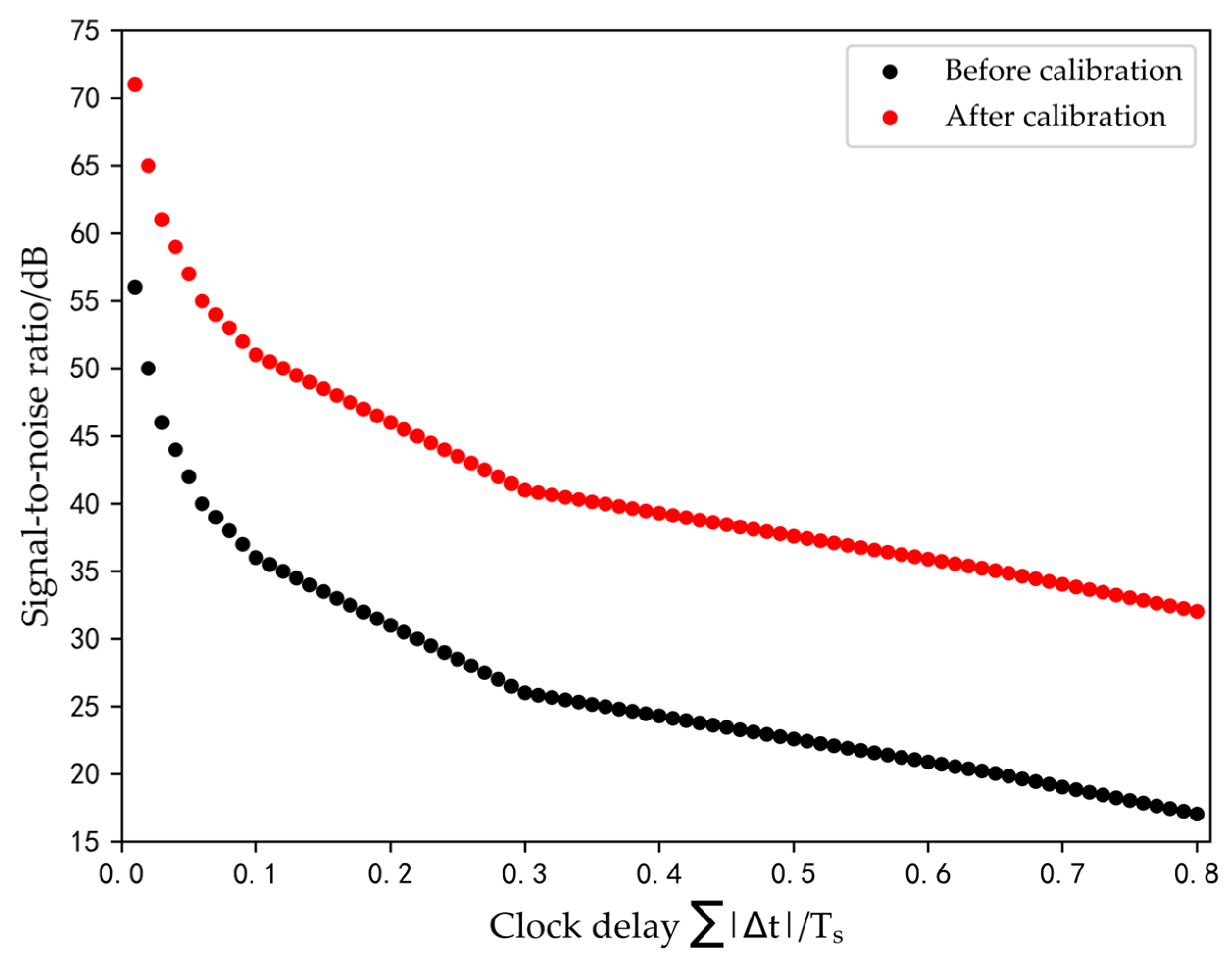
The proposed approach was implemented to determine the clock delay of both two-channel and four-channel TIADC systems. All sampling channels of the TIADC system were sampled with no stray noise present. The input signal was a mixed sine wave, and the clock delays between neighboring channels were not equal. After the calibration of the system based on the clock delay of each channel computed using this method, the improvement effect of the system SINAD for both two-channel and four-channel TIADC systems was analyzed. Figure 8 and Figure 9 show the effect of the improvement, with the abscissa representing the deviation sum of the clock delays of adjacent channels. This approach exhibited the ability to successfully calibrate TIADC systems and was not limited by the number of channels, as SINAD was enhanced by at least 15 dB before and after calibration.

6. Conclusions

This paper proposed an innovative sine wave parameter fitting method: the MQ-RBF interpolation subdivision–least squares method based on optimal shape parameters. Initially, the random walk algorithm was used to select the MQ-RBF interpolation shape parameters for both single-frequency and multi-frequency sinusoids. Exploratory experiments revealed that the angular frequency of a sine wave signal determines its corresponding shape parameters. By using linear regression and the Bayesian optimization–random forest method, the data were trained, and a model for selecting MQ-RBF interpolation shape parameters was created for each sinusoidal signal. The adaptive selection model for MQ-RBF interpolation shape parameters could be used for arbitrary sine waves, making the MQ-RBF interpolation subdivision–least squares method more effective and convenient. The test results showed that this strategy significantly enhanced the accuracy of sine wave parameter estimation. The simulation results demonstrated successful clock delay determination for each channel, without any upper limit on the number of channels, making it a promising solution for the TIADC system channel delay problem. Thus, this method possesses broad application prospects.

Author Contributions

Data curation, J.S.; formal analysis, J.S.; funding acquisition, D.G.; investigation, L.W.; methodology, J.S.; project administration, D.G.; resources, D.G. and L.W.; software, J.S.; supervision, D.G.; validation, L.W.; visualization, L.W.; writing—original draft, J.S. and L.W.; writing—review and editing, J.S. and D.G. All authors have read and agreed to the published version of the manuscript.

Funding

The work of Jian Sun was supported by the National Natural Science Foundation of China (grant No. 11601151).

Data Availability Statement

Not applicable.

Acknowledgments

The authors would like to express their sincere gratitude to the editors and reviewers. The structure and presentation of the paper were greatly improved by their professional and detailed reviews.

Conflicts of Interest

The authors declare no conflict of interest.

References

  1. Franke, R. Scattered data interpolation: Tests of some methods. Math. Comput. 1982, 38, 181–200. [Google Scholar]
  2. Afiatdoust, F.; Esmaeilbeigi, M. Optimal variable shape parameters using genetic algorithm for radial basis function approximation. Ain. Shams Eng. J. 2015, 6, 639–647. [Google Scholar] [CrossRef]
  3. Chen, W.; Hong, Y.; Lin, J. The sample solution approach for determination of the optimal shape parameter in the Multiquadric function of the Kansa method. Comput. Math. Appl. 2018, 75, 2942–2954. [Google Scholar] [CrossRef]
  4. Gu, J.; Jung, J.H. Adaptive Gaussian radial basis function methods for initial value problems: Construction and comparison with adaptive multiquadric radial basis function methods. J. Comput. Appl. Math. 2021, 381, 113036. [Google Scholar] [CrossRef]
  5. Na, J.; Yang, J.; Wu, X.; Guo, Y. Robust adaptive parameter estimation of sinusoidal signals. Automatica 2015, 53, 376–384. [Google Scholar] [CrossRef]
  6. Gavin, H.P. The Levenberg-Marquardt Algorithm for Nonlinear Least Squares Curve-Fitting Problems. Ph.D. Thesis, Duke University, Durham, NC, USA, 2019; p. 19. [Google Scholar]
  7. Niu, G.; Liu, C.; Zhang, J.; Li, X.; Luo, X. Research progress of time-interleaved analog-to-digital converters. Integration 2021, 81, 313–321. [Google Scholar]
  8. Li, X.; Huang, C.; Ding, D.; Wu, J. A review on calibration methods of timing-skew in time-interleaved ADCs. J. Circuits Syst. Comput. 2020, 29, 2030002. [Google Scholar] [CrossRef]
  9. Abbaszadeh, A.; Aghdam, E.N.; Rosado-Muñoz, A. Digital background calibration algorithm and its FPGA implementation for timing mismatch correction of time-interleaved ADC. Analog. Integr. Circuits Signal Process. 2019, 99, 299–310. [Google Scholar] [CrossRef]
  10. Xiong, W.; Zhang, Z.; Sun, L.; Liu, Y.; Liu, H.; Lang, L.; Dong, Y. Fast convergent background calibration technique for timing mismatch in M-channel time-interleaved ADCs. AEU-Int. J. Electron. Commun. 2022, 153, 154282. [Google Scholar] [CrossRef]
  11. Salib, A.; Flanagan, M.F.; Cardiff, B. A high-precision time skew estimation and correction technique for time-interleaved ADCs. IEEE Trans. Circuits Syst. I Regul. Pap. 2019, 66, 3747–3760. [Google Scholar] [CrossRef] [Green Version]
  12. Liu, C.S.; Liu, D. Optimal shape parameter in the MQ-RBF by minimizing an energy gap functional. Appl. Math. Lett. 2018, 86, 157–165. [Google Scholar] [CrossRef]
  13. Luh, L.T. A direct prediction of the shape parameter in the collocation method of solving Poisson equation. Mathematics 2022, 10, 3583. [Google Scholar] [CrossRef]
  14. Ahmad Khan, M.; Altamimi, A.; Hussain Khan, Z.; Shehzad Khattak, K.; Khan, S.; Ullah, A.; Ali, M. Multiquadric radial basis function approximation scheme for solution of total variation based multiplicative noise removal model. Comput. Model. Eng. Sci. 2021, 126, 55–88. [Google Scholar]
  15. Ghalichi, S.S.S.; Amirfakhrian, M.; Allahviranloo, T. An algorithm for choosing a good shape parameter for radial basis functions method with a case study in image processing. Results Appl. Math. 2022, 16, 100337. [Google Scholar] [CrossRef]
  16. Xu, C.; Sun, J.; Wang, C. An image encryption algorithm based on random walk and hyperchaotic systems. Int. J. Bifurc. Chaos 2020, 30, 2050060. [Google Scholar] [CrossRef]
  17. O’Leary, P.; Ninevski, D. Estimating parameters of a sine wave by the method of variable projection. In Proceedings of the 2021 IEEE International Instrumentation and Measurement Technology Conference (I2MTC), Glasgow, UK, 17–20 May 2021; IEEE: Piscataway, NJ, USA, 2021; pp. 1–6. [Google Scholar]
  18. Belega, D.; Petri, D. Fast procedures for accurate parameter estimation of sine-waves affected by noise and harmonic distortion. Digit. Signal Process. 2021, 114, 103035. [Google Scholar] [CrossRef]
  19. Speiser, J.L.; Miller, M.E.; Tooze, J.; Ip, E. A comparison of random forest variable selection methods for classification prediction modeling. Expert Syst. Appl. 2019, 134, 93–101. [Google Scholar] [CrossRef] [PubMed]
  20. Cai, M.; Wang, Y.; Zhao, W.; Shi, X.; Li, T. Study on Local Brittleness of Rock Based on Multiple Linear Regression Method: Case Study of Shahejie Formation. Geofluids 2023, 2023, 6189068. [Google Scholar] [CrossRef]
  21. Wang, Y.; Liao, W.; Chang, Y. Gated recurrent unit network-based short-term photovoltaic forecasting. Energies 2018, 11, 2163. [Google Scholar] [CrossRef] [Green Version]
  22. Pisner, D.A.; Schnyer, D.M. Support vector machine. In Machine Learning; Academic Press: Cambridge, MA, USA, 2020; pp. 101–121. [Google Scholar]
  23. Van Houdt, G.; Mosquera, C.; Nápoles, G. A review on the long short-term memory model. Artif. Intell. Rev. 2020, 53, 5929–5955. [Google Scholar] [CrossRef]
  24. Victoria, A.H.; Maragatham, G. Automatic tuning of hyperparameters using Bayesian optimization. Evol. Syst. 2021, 12, 217–223. [Google Scholar] [CrossRef]
  25. Shen, Y.; Hu, S.; Cai, S.; Chen, M. Software Defect Prediction based on Bayesian Optimization Random Forest. In Proceedings of the 2022 9th International Conference on Dependable Systems and Their Applications (DSA), Wulumuqi, China, 4–5 August 2022; IEEE: Piscataway, NJ, USA, 2022; pp. 1012–1013. [Google Scholar]
  26. Lin, S.; Rothleitner, C.; Rogge, N.; Fröhlich, T. Influences on amplitude estimation using three-parameter sine fitting algorithm in the velocity mode of the Planck-Balance. Acta IMEKO 2020, 9, 40–46. [Google Scholar] [CrossRef]
  27. Belega, D.; Petri, D.; Dallet, D. Amplitude and phase estimation of real-valued sine wave via frequency-domain linear least-squares algorithms. IEEE Trans. Instrum. Meas. 2018, 67, 1065–1077. [Google Scholar] [CrossRef]
  28. Sato, K.; Ishida, T.; Okamoto, T.; Ichikawa, T.; Wei, J.; Nakatani, T.; Zhao, Y.; Katayama, S.; Yamamoto, S.; Kuwana, A.; et al. Revisit to accurate ADC testing with incoherent sampling using proper sinusoidal signal and sampling frequencies. In Proceedings of the 2021 IEEE International Test Conference (ITC), Anaheim, CA, USA, 10–15 October 2021; IEEE: Piscataway, NJ, USA, 2021; pp. 284–288. [Google Scholar]
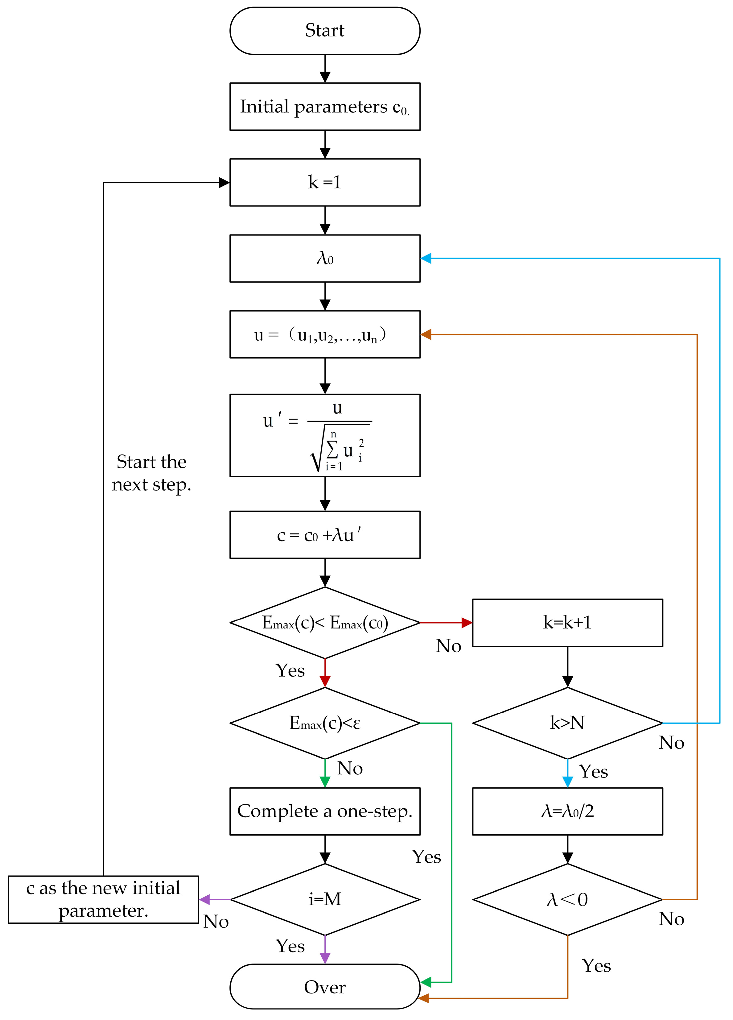
Figure 1. Flow chart of the algorithm.
Mathematics 11 01856 g001
Figure 2. Diagrams of interpolation results of Function (6): (a) Interpolation effect diagram, (b) Interpolation absolute error diagram.
Mathematics 11 01856 g002
Figure 3. Influence of φ on interpolation.
Mathematics 11 01856 g003
Figure 4. Influence of B on interpolation.
Mathematics 11 01856 g004
Figure 5. Schematic diagram of linear model.
Mathematics 11 01856 g005
Figure 6. Interpolation effect diagram of multi-frequency sine signal: (a) Function (13); (b) Function (14); (c) Function (15); (d) Function (16); (e) Function (17).
Mathematics 11 01856 g006aMathematics 11 01856 g006b
Figure 7. Schematic diagram of BO-RF model.
Mathematics 11 01856 g007
Figure 8. Changes in SINAD for a two-channel TIADC.
Mathematics 11 01856 g008
Figure 9. Changes in SINAD for a four-channel TIADC.
Mathematics 11 01856 g009
Table 1. Experimental results of Function (6).
A ω T φ B c o p t M a x E r r o r
1 π 2000.54027 2.28 × 10 7
Table 2. Partial results of Experiment 1.
φ c o p t M a x E r r o r
π / 2 0.54215 2.22 × 10 7
0.031040.54372 2.25 × 10 7
−64.67680.54372 2.31 × 10 7
934.3080.54374 2.26 × 10 7
0.017140.53808 2.29 × 10 7
7.614770.54941 2.27 × 10 7
−0.008290.54299 2.34 × 10 7
−420.9710.54425 2.29 × 10 7
−8.326220.54828 2.26 × 10 7
27.58180.54859 2.30 × 10 7
Table 3. Partial results of A 10 , 10 .
A c o p t M a x E r r o r
−100.54277 2.27 × 10 6
100.54220 2.27 × 10 6
9.724980.54346 2.07 × 10 6
8.657990.54750 1.91 × 10 6
−7.389960.54001 1.57 × 10 6
6.094650.54964 1.29 × 10 6
−5.538810.54770 1.26 × 10 6
4.571210.54895 1.07 × 10 6
3.601340.54661 6.89 × 10 7
−2.395070.54287 5.64 × 10 7
Table 4. Partial results of A 100 , 100 or A 1 , 1 .
A c o p t M a x E r r o r
−1000.54335 2.28 × 10 5
10.54329 2.20 × 10 7
98.54130.54132 2.08 × 10 5
−89.76480.54179 1.99 × 10 5
−74.00790.54297 1.83 × 10 5
−69.09020.54270 1.47 × 10 5
0.533770.54217 1.21 × 10 7
0.408420.54905 1.16 × 10 7
−0.366350.54351 6.03 × 10 8
−0.212470.54329 5.28 × 10 8
Table 5. Partial results of A 1000 , 1000 or A 0.1 , 0.1 .
A c o p t M a x E r r o r
−10000.54306 2.23 × 10 4
0.10.54288 2.23 × 10 8
993.9220.54387 2.13 × 10 4
839.5810.54742 1.98 × 10 4
−710.58490.54194 1.88 × 10 4
674.0220.54008 1.52 × 10 4
0.056560.54846 1.49 × 10 8
0.041630.54921 1.15 × 10 8
0.032440.54245 6.95 × 10 9
Table 6. Partial results of ω = π / k k = 2 , , 10 .
ω T c o p t M a x E r r o r
π / 2 41.08075 2.23 × 10 7
π / 3 61.62036 2.22 × 10 7
π / 4 82.16131 2.26 × 10 7
π / 5 102.70135 2.22 × 10 7
π / 6 123.24163 2.21 × 10 7
π / 7 143.78189 2.24 × 10 7
π / 8 164.32217 2.20 × 10 7
π / 9 184.86243 2.22 × 10 7
π / 10 205.40251 2.23 × 10 7
Table 7. Partial results of ω = k π k = 2 , , 10 .
ω T c o p t M a x E r r o r
2 π 10.27014 2.23 × 10 7
3 π 2/30.18009 2.22 × 10 7
4 π 1/20.13506 2.25 × 10 7
5 π 2/50.10805 2.23 × 10 7
6 π 1/30.09004 2.20 × 10 7
7 π 2/70.07718 2.22 × 10 7
8 π 1/40.06753 2.24 × 10 7
9 π 2/90.06003 2.21 × 10 7
10 π 1/50.05403 2.22 × 10 7
Table 8. Partial results of ω = π / 10 k k = 2 , , 10 .
ω T c o p t M a x E r r o r
π / 20 4010.8055 2.23 × 10 7
π / 30 6016.2075 2.22 × 10 7
π / 40 8021.6114 2.26 × 10 7
π / 50 10027.0127 2.22 × 10 7
π / 60 12034.4161 2.21 × 10 7
π / 70 14037.8192 2.24 × 10 7
π / 80 16043.2217 2.20 × 10 7
π / 90 18048.6246 2.22 × 10 7
π / 100 20054.0269 2.23 × 10 7
Table 9. Partial results of ω = 10 k π k = 2 , , 10 .
ω T c o p t M a x E r r o r
20 π 1/100.02701 2.24 × 10 7
30 π 1/150.01802 2.26 × 10 7
40 π 1/200.01351 2.22 × 10 7
50 π 1/250.01084 2.20 × 10 7
60 π 1/300.00904 2.20 × 10 7
70 π 1/350.00772 2.21 × 10 7
80 π 1/400.00675 2.22 × 10 7
90 π 1/450.00603 2.26 × 10 7
100 π 1/500.00541 2.28 × 10 7
Table 10. Test function.
No.Function
1 f x = 0.0478 sin 159.58 x + 0.6578 + 0.6276
2 f x = 0.7024 sin 60.166 x 674.62 + 0.0050
3 f x = 7986.9 sin 29.568 x 0.7312 + 0.48157
4 f x = 8.4447 sin 7.0582 x 8667.2 + 0.91681
5 f x = 0.0047 sin 4.1222 x 0.0750 + 0.0022
6 f x = 953.89 sin 0.8483 x + 0.0384 + 0.2979
7 f x = 0.0744 sin 0.5686 x 0.8661 + 0.0089
8 f x = 686.43 sin 0.0710 x 0.0095 + 0.78021
9 f x = 0.9193 sin 0.0277 x + 5606.2 + 0.36172
10 f x = 4337.9 sin 0.0047 x 9263.1 + 0.4201
11 f x = 574.92 sin 0.00063 x + 68.223 + 0.35844
12 f x = 0.6012 sin 0.0002 x + 0.5863 + 0.026393
Table 11. Results of verification experiment.
No. c o p t M a x E r r o r
ModelAlgorithmModelAlgorithm
10.1775330.176142 4.27 × 10 6 4.27 × 10 6
20.1952700.193445 2.31 × 10 7 2.31 × 10 7
30.2247310.223564 2.84 × 10 3 2.83 × 10 3
40.4094840.417821 2.44 × 10 5 2.43 × 10 5
50.5823340.582365 7.17 × 10 9 7.17 × 10 9
62.1860332.187564 3.06 × 10 7 3.06 × 10 7
73.1793143.278312 4.31 × 10 8 4.30 × 10 8
824.2923724.78781 2.26 × 10 2 2.26 × 10 2
962.0049261.98731 9.74 × 10 5 9.74 × 10 5
10364.6165365.8971 1.57 × 10 3 1.59 × 10 3
112719.0812721.782 9.62 × 10 3 9.61 × 10 3
128564.7458566.898 6.12 × 10 5 6.10 × 10 5
Table 12. Evaluation results of regression model.
ModelTime (min) R 2 MSEMAE
RF20410.9295780.3487870.457872
LSTM20920.8324511.3237242.876757
GRU19820.8078431.6343122.487212
SVR27810.7389725.6242457.997901
MLR18670.65893113.6311216.89777
Table 13. Model accuracy evaluation results.
ModelEvaluation IndexResult
BO-RFTime (min)2144
R 2 0.9684
MSE0.1956826
MAE0.38006
Table 14. Test function.
No.Sine WaveSample Point
13 f x = 5 cos 41 x + π / 6 + 0.3 25
14 f x = 2 sin 2 x + π / 3 + 0.1 58
15 f x = 10 sin 0.16 x + 5 + 0.7 101
Table 15. Fitting value and absolute error of MQ-LS.
NO.Result A φ B
13Fitting4.9999998380.5235987920.300000818
AE 1.62 × 10 7 1.64 × 10 8 8.18 × 10 7
14Fitting2.0000000171.0471975470.100000024
AE 1.70 × 10 8 4.19 × 10 9 2.40 × 10 8
15Fitting9.9999995135.0000022170.700000034
AE 4.86 × 10 7 2.22 × 10 6 3.40 × 10 8
Table 16. Fitting value and absolute error of LS.
NO.Result A φ B
13Fitting4.9999788840.5236034030.300006379
AE 2.11 × 10 5 4.63 × 10 6 6.38 × 10 6
14Fitting1.9999992861.0471985650.099999622
AE 7.14 × 10 7 1.01 × 10 6 3.78 × 10 7
15Fitting10.000030795.0000174210.700000058
AE 3.08 × 10 5 1.74 × 10 5 5.80 × 10 8
Disclaimer/Publisher’s Note: The statements, opinions and data contained in all publications are solely those of the individual author(s) and contributor(s) and not of MDPI and/or the editor(s). MDPI and/or the editor(s) disclaim responsibility for any injury to people or property resulting from any ideas, methods, instructions or products referred to in the content.