Numerical Method for a Cauchy Problem for Multi-Dimensional Laplace Equation with Bilateral Exponential Kernel

Abstract

This study examined a Cauchy problem for a multi-dimensional Laplace equation with mixed boundary. This problem is severely ill-posed in the sense of Hadamard. To solve this problem, a mollification approach is suggested based on a bilateral exponential kernel and this is a new approach. The stable error estimates are obtained under the priori and posteriori rule, in which the numerical findings are much influenced by the unknown a priori information. An error estimate between the exact and regular solution is given. A numerical experiment of interest reveals that our procedure is efficient and stable for perturbation noise in the data.

1. Introduction

The Laplace equation’s inverse problem appears in numerous engineering and physical areas, for example, cardiology, geophysics, seismology, and so on [1,2,3]. The Cauchy problem of the Laplace equation plays a crucial role in all inverse problems of elliptic partial differential equations. Particularly, the Cauchy problem for the multi-dimensional Laplace equation. The Laplace equation’s inverse problem is severely ill-posed in the sense of Hadamard, where a tiny deviation in the data can cause a substantial error in the solution [4]. Thus, we require to use a regularization method to solve the ill-posed problem. Several approaches have been provided. The readers can consult the Tikhonov regularization [5], quasi-reversibility [6], wavelet [7], conjugate gradient [8], the central difference [9], Fourier regularization [10], and mollification [11,12,13] methods, etc.

The primary step of the mollification method is to build a mollification operator by convolving a kernel function with the determined data. Manselli, Miller [14] and Murio [15,16] constructed mollification operators using the Weierstrass kernel to address some inverse heat conduction problems (IHCP). The Cauchy problem of an elliptic equation employing the Gaussian kernel function has been reported [17,18,19,20,21]. Hào [22,23,24] adopted the de la Vallée Poussin kernel and Dirichlet kernel to solve some types of two-dimensional equations, such as the two-dimensional Laplace equation. However, the multi-dimensional case was not considered. Furthermore, the analytical methods employed for error estimation do not generalize well to multi-dimensional cases. In our practical application, we often need to consider the application of the Laplace equation in multi-dimensional cases. This is why we adopt the mollification method based on the bilateral exponential kernel to solve the multi-dimensional Laplace problem. The refs. [25,26] are related to the work.

The primary aim of this study is to solve the multi-dimensional Laplace equation’s inverse problem with mixed boundary conditions. To guarantee solvability for the inverse problem offered, a regularization method using the bilateral exponential kernel is presented and we will show that our approach is stable and effective in $0<x<1$ and at boundary $x=1$.

The study is organized as follows: In Section 2, the ill-posed of the problem (1) is illustrated. In Section 3, we introduce the bilateral exponential kernel and its certain properties and suggest our mollification method. In Section 4, some error estimate findings are given in $0<x<1$ and $x=1$. The efficiency of the approach is depicted in Section 5 through numerical experiments. Section 6 presents the summary and conclusions.

2. Model Problem and Its Ill-Posedness

We consider the following Cauchy problem for a multi-dimensional Laplace equation with a mixed boundary condition:

Consider the following:

$$\left\{\begin{array}{c}\Delta u(x,\mathbf{y})=0,0<x<1,\mathbf{y}\in R^n,\hfill \\ u(0,\mathbf{y})=\phi (\mathbf{y}),\mathbf{y}\in R^n,\hfill \\ u_x(0,\mathbf{y})=\psi (\mathbf{y}),\mathbf{y}\in R^n.\hfill \end{array}\right.$$

(1)

where $\Delta =\frac{{\partial }^2}{\partial y_1^2}+\frac{{\partial }^2}{\partial y_2^2}+\dots +\frac{{\partial }^2}{\partial y_n^2}$ is a multi-dimensional Laplace operator. We need to obtain the solution $u(x,\mathbf{y})$ from the data $\phi (\mathbf{y}),\psi (\mathbf{y})$, but $\phi (\mathbf{y}),\psi (\mathbf{y})$ can only be measured and there are measurement errors. We know some data functions ${\phi }^{\delta }(\mathbf{y}),{\psi }^{\delta }(\mathbf{y})$ such that

$$\begin{array}{c}\hfill \parallel {\phi }^{\delta }-\phi \parallel \le \delta ,\parallel {\psi }^{\delta }-\psi \parallel \le \delta .\end{array}$$

(2)

Here, constant $\delta >0$ represents the level of error,

$${\parallel f(.)\parallel }_{H^p}:=({\int }_{-\infty }^{+\infty }{(1+{\xi }^2)}^p|\widehat{f}(\xi ){{|}^{2}d\xi )}^{\frac{1}{2}}.$$

$\widehat{f}(\xi )$ is the Fourier transform of function $f(\mathbf{y})$ for the $y\in R^n$,

$$\widehat{f}(\xi )=\frac{1}{{(2\pi )}^{n/2}}{\int }_{R^n}f(y)e^{-i\xi .y}dy,y\in R^n.$$

The inverse Fourier transform of function $f(\mathbf{y})$ is

$$f(y)=\frac{1}{{(2\pi )}^{n/2}}{\int }_{R^n}\widehat{f}(\xi )e^{i\xi .y}d\xi .$$

If $p=0$, then $H^0(R^n)=L^2(R^n).$

Obviously, the solution of the problem (1) is the sum of solutions for the following two Cauchy problems:

$$\left\{\begin{array}{c}\Delta u_1(x,\mathbf{y})=0,0<x<1,\mathbf{y}\in R^n,\hfill \\ u_1(0,\mathbf{y})=\phi (\mathbf{y}),\mathbf{y}\in R^n,\hfill \\ {(u_1)}_x(0,\mathbf{y})=0,\mathbf{y}\in R^n\hfill \end{array}\right.$$

(3)

and

$$\left\{\begin{array}{c}\Delta u_2(x,\mathbf{y})=0,0<x<1,\mathbf{y}\in R^n,\hfill \\ u_2(0,\mathbf{y})=0,\mathbf{y}\in R^n,\hfill \\ {(u_2)}_x(0,\mathbf{y})=\psi (\mathbf{y}),\mathbf{y}\in R^n\hfill \end{array}\right.$$

(4)

Using the Fourier transform for the variable $\mathbf{y}\in R^n$ to the problems (3) and (4), we obtain

$$\left\{\begin{array}{c}{\widehat{(u_1)}}_{xx}={\xi }^2{\widehat{u}}_1,0<x<1,\xi \in R^n,\hfill \\ \widehat{u_1}(0,\xi )=\widehat{\phi }(\xi ),\xi \in R^n,\hfill \\ {(\widehat{u_1})}_x(0,\xi )=0,\xi \in R^n\hfill \end{array}\right.$$

(5)

and

$$\left\{\begin{array}{c}{\widehat{(u_2)}}_{xx}={\xi }^2\widehat{u_2},0<x<1,\xi \in R^n,\hfill \\ \widehat{u_2}(0,\xi )=0,\xi \in R^n,\hfill \\ {(\widehat{u_2})}_x(0,\xi )=\widehat{\psi }(\xi ),\xi \in R^n\hfill \end{array}\right.$$

(6)

The solution of problem (5) is

$$\begin{array}{c}\hfill {\widehat{u}}_1(x,\xi )=cosh(x|\xi |)\widehat{\phi }(\xi ).\end{array}$$

(7)

So, the solution of problem (3) is

$$\begin{array}{c}\hfill u_1(x,\mathbf{y})=\frac{1}{{(2\pi )}^{\frac{n}{2}}}{\int }_{R^n}cosh(x|\xi |)\widehat{\phi }(\xi )e^{i\xi .y}d\xi .\end{array}$$

(8)

Similarly, for problem (6), the solution is

$$\begin{array}{c}\hfill {\widehat{u}}_2(x,\xi )=\frac{sinh(x|\xi |)}{|\xi |}\widehat{\psi }(\xi ).\end{array}$$

(9)

For problem (4), the solution is

$$\begin{array}{c}\hfill u_2(x,\mathbf{y})=\frac{1}{{(2\pi )}^{\frac{n}{2}}}{\int }_{R^n}\frac{sinh(x|\xi |)}{|\xi |}\widehat{\psi }(\xi )e^{i\xi .y}d\xi .\end{array}$$

(10)

Obviously, the $cosh(x|\xi |)$ and $\frac{sinh(x|\xi |)}{|\xi |}$ are unbounded with respect to variable $\xi$, and a small perturbation in the measured data ${\phi }^{\delta }(\mathbf{y})$ and ${\psi }^{\delta }(\mathbf{y})$ may cause a dramatically large error in the solutions $u_1(x,\mathbf{y})$$,u_2(x,\mathbf{y})$. So problem (1) is severely ill-posed.

3. Bilateral Exponential Kernel and Auxiliary Results

The multi-dimensional even bilateral exponential function is defined as:

$$\begin{array}{c}\hfill V_{\mu }(x):=\frac{\mu }{2}{e}^{-\mu |x|},0<\mu <1,x\in R^n.\end{array}$$

(11)

and there is

$$\begin{array}{c}\hfill {\int }_{R_n}{V}_{\mu }(x)dx:={\int }_{R_n}\frac{\mu }{2}{e}^{-\mu |x|}dx=1,0<\mu <1.\end{array}$$

Here, $0<\mu <1$ is called a regularization parameter and we define the regularization operator ${\omega }_{\mu }$ as the following:

$$\begin{array}{c}\hfill {\omega }_{\mu }f(x):=V_{\mu }\ast f(x)={\int }_{R^n}{V}_{\mu }(t)f(x-t)dt={\int }_{R^n}{V}_{\mu }(x-t)f(t)dt.\end{array}$$

(12)

Fourier transform of $V_{\mu }(x)$ is

$$\begin{array}{c}\hfill {\widehat{V}}_{\mu }(\xi )={\int }_{R^n}\frac{\mu }{2}{e}^{-\mu |x|}{e}^{-i\xi x}dx=\frac{{\mu }^2}{{\mu }^2+{\xi }^2}.\end{array}$$

(13)

Lemma 1.

Letting $V,f\in L^2(R^n)$, we have

$$\begin{array}{c}\hfill \widehat{(V\ast f)}(\xi )={(2\pi )}^{n/2}\widehat{V}(\xi )\widehat{f}(\xi ).\end{array}$$

(14)

We reconstruct the function ${\phi }^{\delta }(\mathbf{y}),{\psi }^{\delta }(\mathbf{y})$ by $(V_{\mu }\ast {\phi }^{\delta })(\mathbf{y}),(V_{\mu }\ast {\psi }^{\delta })(\mathbf{y})$, respectively, to solve the problems (3) and (4) with the data ${\phi }^{\delta }(\mathbf{y}),{\psi }^{\delta }(\mathbf{y})$ and have the following two problems with modified data:

$$\left\{\begin{array}{c}\Delta u_1^{\mu ,\delta }(x,\mathbf{y})=0,0<x<1,y\in R^n,\hfill \\ u_1^{\mu ,\delta }(0,\mathbf{y})=(V_{\mu }\ast {\phi }^{\delta })(\mathbf{y}),y\in R^n,\hfill \\ {(u_1^{\mu ,\delta })}_x(0,\mathbf{y})=0,y\in R^n\hfill \end{array}\right.$$

(15)

and

$$\left\{\begin{array}{c}\Delta u_2^{\mu ,\delta }(x,\mathbf{y})=0,0<x<1,y\in R^n,\hfill \\ u_2^{\mu ,\delta }(0,\mathbf{y})=0,y\in R^n,\hfill \\ {(u_2^{\mu ,\delta })}_x(0,\mathbf{y})=(V_{\mu }\ast {\psi }^{\delta }(\mathbf{y}),y\in R^n\hfill \end{array}\right.$$

(16)

The solution of problem (15) can be formulated in the frequency domain:

$${\widehat{u}}_1^{\mu ,\delta }(x,\xi )=(\widehat{V_{\mu }\ast {\phi }^{\delta }})(\xi )cosh(x|\xi |)=\frac{{(2\pi )}^{n/2}{\mu }^2}{{\mu }^2+{\xi }^2}{\widehat{\phi }}^{\delta }(\xi )cosh(x|\xi |).$$

Similarly, the solution of problem (16) is:

$${\widehat{u}}_2^{\mu ,\delta }(x,\xi )=(\widehat{V_{\mu }\ast {\psi }^{\delta }})(\xi )\frac{sinh(x|\xi |)}{|\xi |}=\frac{{(2\pi )}^{n/2}{\mu }^2}{{\mu }^2+{\xi }^2}{\widehat{\psi }}^{\delta }(\xi )\frac{sinh(x|\xi |)}{|\xi |}.$$

Thus, the regularization approximation solution of problem (1) in the frequency domain is:

$${\widehat{u}}^{\mu ,\delta }(x,\xi )=(\widehat{V_{\mu }\ast {\phi }^{\delta }})(\xi )cosh(x|\xi |)+(\widehat{V_{\mu }\ast {\psi }^{\delta }})(\xi )\frac{sinh(x|\xi |)}{|\xi |}$$

Equivalently,

$$u^{\mu ,\delta }(x,\mathbf{y})=\frac{1}{{(2\pi )}^{n/2}}{\int }_{R^n}[(\widehat{V_{\mu }\ast {\phi }^{\delta }})(\xi )cosh(x|\xi |)+(\widehat{V_{\mu }\ast {\psi }^{\delta }})(\xi )\frac{sinh(x|\xi |)}{|\xi |}]e^{i\xi x}d\xi .$$

Lemma 2

(see [27]). For $0<x\le 1$$,\xi >0$ then the following inequalities hold:

$$\begin{array}{cc}\hfill & (1)cosh(x|\xi |)\le e^{x|\xi |};\hfill \\ \hfill & (2)\frac{sinh(x|\xi |)}{|\xi |}\le e^{x|\xi |};\hfill \\ \hfill & (3)\frac{cosh(x|\xi |)}{cosh|\xi |}\le 2e^{-(1-x)|\xi |};\hfill \\ \hfill & (4)\frac{sinh(x|\xi |)}{sinh|\xi |}\le e^{-(1-x)|\xi |}.\hfill \end{array}$$

Lemma 3.

If $0<\mu <1$, then the following inequalities hold:

$$\begin{array}{c}\hfill \underset{\xi \in R}{sup}|(1-\frac{{(2\pi )}^{n/2}{\mu }^2}{{\mu }^2+{\xi }^2}){(1+{\xi }^2)}^{-\frac{p}{2}}|\le max\{{(2\pi )}^{n/2}{\mu }^p,{(2\pi )}^{n/2}{\mu }^2\}.\end{array}$$

Proof. 

Define

$$E(\xi ):=(1-\frac{{(2\pi )}^{n/2}{\mu }^2}{{\mu }^2+{\xi }^2}){(1+{\xi }^2)}^{-\frac{p}{2}}.$$

The proof of the above inequality is divided into three cases:

(i): If $|\xi |\ge {\xi }_0=\frac{1}{\mu }$, we have

$$\begin{array}{cc}\hfill |E(\xi )|\le |(1-\frac{{(2\pi )}^{n/2}{\mu }^2}{{\mu }^2+{\xi }^2}){(1+{\xi }^2)}^{-\frac{p}{2}}|& \le |\frac{{(2\pi )}^{n/2}{\mu }^2}{{\mu }^2{\xi }^p}|\hfill \\ \hfill \le {(2\pi )}^{n/2}{\xi }_0^{-p}={(2\pi )}^{n/2}{\mu }^p.\end{array}$$

(ii): If $1<|\xi |<{\xi }_0$,

$$|E(\xi )|=|(1-\frac{{(2\pi )}^{n/2}{\mu }^2}{{\mu }^2+{\xi }^2}){(1+{\xi }^2)}^{-\frac{p}{2}}|\le \frac{{(2\pi )}^{n/2}{\mu }^2}{{\xi }^{p+2}}\le {(2\pi )}^{n/2}{\mu }^2.$$

(iii): If $|\xi |\le 1$,

$$\begin{array}{cc}\hfill |E(\xi )|=|(1-\frac{{(2\pi )}^{n/2}{\mu }^2}{{\mu }^2+{\xi }^2}){(1+{\xi }^2)}^{-\frac{p}{2}}|& \le |\frac{{\xi }^2-2{\mu }^2}{{\xi }^2}|\hfill \\ \hfill \le |1-2{\mu }^2{|\le (2\pi )}^{n/2}{\mu }^2.\end{array}$$

From the above, the Lemma is proved. □

4. Regularization and Error Estimates

4.1. An a Priori Approach for Problem (1)

In the following, we will give stable error estimates between the regularization approximate solution and the exact solution for problem (1) in $0<x<1$ and at $x=1$, respectively.

We need to follow a priori bound

$$\begin{array}{c}\hfill \Vert u_1{(1,.)\Vert }_{H^0(R^n)}\le E,{\Vert u_2(1,.)\Vert }_{H^0(R^n)}\le E,\end{array}$$

(17)

here, $E$ is a positive constant.

In this part, we will give the stable convergence estimate findings in the case of $0<x<1.$

Theorem 1.

When $0<x<1$$,u(x,\mathbf{y})$ is the exact solution of problem (1), and $u^{\mu ,\delta }(x,\mathbf{y})$ is the regular approximation solution of problem (1). The inequalities (2) and (17) hold, then we have

$$\begin{array}{c}\hfill \parallel u-u^{\mu ,\delta }\parallel \le \frac{3}{2}E{(2\pi )}^{n/2}\mu \frac{(x-1)}{e}+2{(2\pi )}^{n/2}\mu xe\delta .\end{array}$$

(18)

When the regularization parameter $\mu$ is chosen as

$$\begin{array}{c}\hfill \mu =\frac{\delta }{E},\end{array}$$

(19)

we have

$$\begin{array}{c}\hfill \parallel u-u^{\mu ,\delta }\parallel \le \frac{3}{2}{(2\pi )}^{n/2}\frac{(x-1)\delta }{e}+2{(2\pi )}^{n/2}\frac{{\delta }^{2}xe}{E}\to 0as\delta \to 0.\end{array}$$

(20)

Proof. 

Using the triangle inequality, we have

$$\begin{array}{c}\hfill \parallel u-u^{\mu ,\delta }\parallel \le \parallel u_1-u_1^{\mu ,\delta }\parallel +\parallel u_2-u_2^{\mu ,\delta }\parallel .\end{array}$$

(21)

According Parseval equality and Lemma 2, there is

$$\begin{array}{cc}\hfill \parallel u_1-u_1^{\mu ,\delta }\parallel & =\parallel {\widehat{u}}_1-{\widehat{u}}_1^{\mu ,\delta }\parallel \le \parallel {\widehat{u}}_1-{\widehat{u}}_1^{\mu ,0}\parallel +\parallel {\widehat{u}}_1^{\mu ,0}-{\widehat{u}}_1^{\mu ,\delta }\parallel \hfill \\ \hfill & =\parallel (1-\frac{{(2\pi )}^{n/2}{\mu }^2}{{\mu }^2+{\xi }^2})\widehat{\phi }(\xi )cosh(x|\xi |)\parallel \hfill \\ \hfill & +\parallel \frac{{(2\pi )}^{n/2}{\mu }^2}{{\mu }^2+{\xi }^2}cosh(x|\xi |)(\widehat{\phi }(\xi )-\widehat{{\phi }^{\delta }(\xi )})\parallel \hfill \\ \hfill & =\parallel (1-\frac{{(2\pi )}^{n/2}{\mu }^2}{{\mu }^2+{\xi }^2})cosh(x|\xi |)\frac{1}{cosh(|\xi |)}{\widehat{u}}_1(1,\xi )\parallel \hfill \\ \hfill & +\parallel \frac{{(2\pi )}^{n/2}{\mu }^2}{{\mu }^2+{\xi }^2}cosh(x|\xi |)\parallel \delta \hfill \\ \hfill & \le E\underset{\xi \in R^n}{sup}|(1-\frac{{(2\pi )}^{n/2}{\mu }^2}{{\mu }^2+{\xi }^2})\frac{cosh(x|\xi |)}{cosh(|\xi |)}|+\delta \underset{\xi \in R^n}{sup}|(\frac{{(2\pi )}^{n/2}{\mu }^2}{{\mu }^2+{\xi }^2}cosh(x|\xi |))|\hfill \\ \hfill & \le E\underset{\xi \in R^n}{sup}|(1-\frac{{(2\pi )}^{n/2}{\mu }^2}{{\mu }^2+{\xi }^2})2e^{-(1-x)|\xi |}|+\delta \underset{\xi \in R^n}{sup}|\frac{{(2\pi )}^{n/2}{\mu }^2}{{\mu }^2+{\xi }^2}{e}^{x|\xi |}|\hfill \\ \hfill & \le E\underset{\xi \in R^n}{sup}|A(\xi )|+\delta \underset{\xi \in R^n}{sup}|B(\xi )|\hfill \end{array}$$

$$|A(\xi )|\le |\frac{{(2\pi )}^{n/2}{\mu }^2-({\mu }^2+{\xi }^2)}{{\mu }^2+{\xi }^2})\frac{2}{e^{(1-x)|\xi |}}{|\le |(2\pi )}^{n/2}\mu \frac{1}{\xi e^{(1-x)\xi }}|.$$

Letting

$$t_1(\xi )=\frac{1}{\xi e^{(1-x)\xi }},$$

when $t_1^{\prime }(\xi )=0$, we obtain

$$\xi =\frac{1}{(x-1)}.$$

By verifying that $\xi =\frac{1}{(x-1)}$ is the maximum point of the function $\frac{1}{\xi e^{(1-x)\xi }}$, and since the maximum point is unique, we can obtain

$$\begin{array}{c}\hfill |A(\xi )|\le {(2\pi )}^{n/2}\mu \frac{(x-1)}{e}.\end{array}$$

(22)

Similarly,

$$|B(\xi )|\le {(2\pi )}^{n/2}\mu \frac{e^{x\xi }}{\xi }$$

Letting

$$t_2(\xi )=\frac{e^{x\xi }}{\xi },$$

we have

$$t_2^{\prime }(\xi )=\frac{x{e}^{x\xi }\xi -e^{x\xi }}{{\xi }^2}.$$

Letting $t_2^{\prime }(\xi )=0$, we obtain

$$\xi =\frac{1}{x}.$$

$\xi =\frac{1}{x}$ is the maximum point of the function, and since the maximum point is unique, we can obtain

$$\begin{array}{c}\hfill |B(\xi )|\le {(2\pi )}^{n/2}\mu t_2(\frac{1}{x})\le {(2\pi )}^{n/2}\mu xe.\end{array}$$

(23)

Combining the estimates of (22) and (23), we obtain

$$\begin{array}{c}\hfill \parallel u_1-u_1^{\mu ,\delta }{\parallel \le E(2\pi )}^{n/2}\mu \frac{(x-1)}{e}+\delta {(2\pi )}^{n/2}\mu xe.\end{array}$$

(24)

In the same way, there is

$$\begin{array}{cc}\hfill \parallel u_2-u_2^{\mu ,\delta }\parallel & =\parallel {\widehat{u}}_2-{\widehat{u}}_2^{\mu ,\delta }\parallel \le \parallel {\widehat{u}}_2-{\widehat{u}}_2^{\mu ,0}\parallel +\parallel {\widehat{u}}_2^{\mu ,0}-{\widehat{u}}_2^{\mu ,\delta }\parallel \hfill \\ \hfill & =\parallel (1-\frac{{(2\pi )}^{n/2}{\mu }^2}{{\mu }^2+{\xi }^2})\widehat{\psi }(\xi )\frac{sinh(x|\xi |)}{|\xi |}\parallel \hfill \\ \hfill & +\parallel \frac{{(2\pi )}^{n/2}{\mu }^2}{{\mu }^2+{\xi }^2}\frac{sinh(x|\xi |)}{|\xi |}(\widehat{\psi }(\xi )-\widehat{{\psi }^{\delta }(\xi )})\parallel \hfill \\ \hfill & =\parallel (1-\frac{{(2\pi )}^{n/2}{\mu }^2}{{\mu }^2+{\xi }^2})\frac{sinh(x|\xi |)}{|\xi |}\frac{|\xi |}{sinh(|\xi |)}{\widehat{u}}_2(1,\xi )\parallel \hfill \\ \hfill & +\parallel \frac{{(2\pi )}^{n/2}{\mu }^2}{{\mu }^2+{\xi }^2}\frac{sinh(x|\xi |)}{|\xi |}\parallel \delta \hfill \\ \hfill & \le E\underset{\xi \in R^n}{sup}(1-\frac{{(2\pi )}^{n/2}{\mu }^2}{{\mu }^2+{\xi }^2})\frac{sinh(x|\xi |)}{sinh(|\xi |)}+\delta \underset{\xi \in R^n}{sup}(\frac{{(2\pi )}^{n/2}{\mu }^2}{{\mu }^2+{\xi }^2}\frac{sinh(x|\xi |)}{|\xi |}\hfill \\ \hfill & \le E\underset{\xi \in R^n}{sup}|(1-\frac{{(2\pi )}^{n/2}{\mu }^2}{{\mu }^2+{\xi }^2})e^{-(1-x)|\xi |}|+\delta \underset{\xi \in R^n}{sup}|\frac{{(2\pi )}^{n/2}{\mu }^2}{{\mu }^2+{\xi }^2}{e}^{x|\xi |}|\hfill \\ \hfill & \le E\underset{\xi \in R^n}{sup}|C(\xi )|+\delta \underset{\xi \in R^n}{sup}|D(\xi )|\hfill \end{array}$$

Similarly, we obtain

$$|C(\xi )|=\frac{1}{2}|A(\xi )|\le \frac{1}{2}{(2\pi )}^{n/2}\mu \frac{(x-1)}{e},|D(\xi )|=|B(\xi )|\le {(2\pi )}^{n/2}\mu xe$$

$$\begin{array}{c}\hfill \parallel u_2-u_2^{\mu ,\delta }\parallel \le E\frac{1}{2}{(2\pi )}^{n/2}\mu \frac{(x-1)}{e}+\delta {(2\pi )}^{n/2}\mu xe.\end{array}$$

(25)

Combining the results of (24) and (25), we obtain (18). The proof of the theorem is completed. □

When $x=1$, we propose a stronger priori bound as follows:

$$\begin{array}{c}\hfill {\parallel u(1,.)\parallel }_{H^p}\le E_p.\end{array}$$

(26)

Theorem 2.

When $x=1$, $u(x,\mathbf{y})$ and $u^{\mu ,\delta }(x,\mathbf{y})$ is the exact and the regular approximation solution of problem (1). The inequalities (2) and (26) hold, then we have

$$\begin{array}{c}\hfill \parallel u-u^{\mu ,\delta }\parallel \le 2E_{p}max\{{(2\pi )}^{n/2}{\mu }^p,{(2\pi )}^{n/2}{\mu }^2\}+2{(2\pi )}^{n/2}\mu e\delta .\end{array}$$

(27)

When the regularization parameter $\mu$ chosen as

$$\begin{array}{c}\hfill \mu =\frac{\delta }{E_p},\end{array}$$

(28)

we have the following error estimates:

$$\begin{array}{cc}\hfill \parallel u-u^{\mu ,\delta }\parallel & \le 2E_{p}max\{{(2\pi )}^{n/2}{(\frac{\delta }{E_p})}^p,{(2\pi )}^{n/2}{(\frac{\delta }{E_p})}^2\}\hfill \\ \hfill & +2{(2\pi )}^{n/2}\frac{e{\delta }^2}{E_p}\to 0as\delta \to 0.\hfill \end{array}$$

(29)

Proof. 

Using the triangle inequality, we have

$$\begin{array}{c}\hfill \parallel u(1,.)-u^{\mu ,\delta }(1,.)\parallel \le \parallel u_1(1,.)-u_1^{\mu ,\delta }(1,.)\parallel +\parallel u_2(1,.)-u_2^{\mu ,\delta }(1,.)\parallel .\end{array}$$

(30)

According Parseval equality and Lemma 2, there is

$$\begin{array}{cc}\hfill \parallel u_1(1,.)-u_1^{\mu ,\delta }(1,.)\parallel & =\parallel {\widehat{u}}_1(1,.)-{\widehat{u}}_1^{\mu ,\delta }(1,.)\parallel \le \parallel {\widehat{u}}_1(1,.)-{\widehat{u}}_1^{\mu ,0}(1,.)\parallel \hfill \\ \hfill & +\parallel {\widehat{u}}_1^{\mu ,0}(1,.)-{\widehat{u}}_1^{\mu ,\delta }(1,.)\parallel \hfill \\ \hfill & =\parallel (1-\frac{{(2\pi )}^{n/2}{\mu }^2}{{\mu }^2+{\xi }^2})\widehat{\phi }(\xi )cosh(|\xi |)\parallel \hfill \\ \hfill & +\parallel \frac{{(2\pi )}^{n/2}{\mu }^2}{{\mu }^2+{\xi }^2}cosh(|\xi |)(\widehat{\phi }(\xi )-\widehat{{\phi }^{\delta }(\xi )})\parallel \hfill \\ \hfill & =\parallel (1-\frac{{(2\pi )}^{n/2}{\mu }^2}{{\mu }^2+{\xi }^2}){(1+{\xi }^2)}^{-\frac{p}{2}}{(1+{\xi }^2)}^{\frac{p}{2}}{\widehat{u}}_1(1,\xi )\parallel \hfill \\ \hfill & +\parallel \frac{{(2\pi )}^{n/2}{\mu }^2}{{\mu }^2+{\xi }^2}cosh(|\xi |)\parallel \delta \hfill \\ \hfill & \le E_p\underset{\xi \in R^n}{sup}|\frac{{\mu }^2+{\xi }^2-{(2\pi )}^{n/2}{\mu }^2}{{\mu }^2+{\xi }^2}\frac{1}{{\xi }^p}|+\delta \underset{\xi \in R^n}{sup}|\frac{{(2\pi )}^{n/2}{\mu }^2}{{\mu }^2+{\xi }^2}{e}^{|\xi |}|\hfill \\ \hfill & \le E_p\underset{\xi \in R^n}{sup}|E(\xi )|+\delta \underset{\xi \in R^n}{sup}|F(\xi )|\hfill \end{array}$$

Using Lemma 3, we known

$$\begin{array}{c}\hfill |E(\xi )|\le max\{{(2\pi )}^{n/2}{\mu }^p,{(2\pi )}^{n/2}{\mu }^2\}.\end{array}$$

(31)

$$\begin{array}{c}\hfill |F(\xi )|\le {(2\pi )}^{n/2}\mu \frac{e^{|\xi |}}{\xi }\end{array}$$

Letting $t_3(\xi )=\frac{e^{\xi }}{\xi }$, we have $t_3^{\prime }(\xi )=0$ and we obtain

$$\xi =1.$$

Clearly $,\xi =1$ is the maximum point of the function, and since the maximum point is unique, we can obtain

$$\begin{array}{c}\hfill |F(\xi )|\le {(2\pi )}^{n/2}\mu e.\end{array}$$

(32)

Combining the estimates of (31) and (32), we obtain

$$\begin{array}{c}\hfill \parallel u_1(1,.)-u_1^{\mu ,\delta }(1,.)\parallel \le E_{p}max\{{(2\pi )}^{n/2}{\mu }^p,{(2\pi )}^{n/2}{\mu }^2\}+{(2\pi )}^{n/2}\mu e\delta .\end{array}$$

(33)

Similarly, taking a similar process of the error estimate as $\parallel u_1(1,.)-u_1^{\mu ,\delta }(1,.)\parallel$, we can obtain

$$\begin{array}{c}\hfill \parallel u_2(1,.)-u_2^{\mu ,\delta }(1,.)\parallel \le E_{p}max\{{(2\pi )}^{n/2}{\mu }^p,{(2\pi )}^{n/2}{\mu }^2\}+{(2\pi )}^{n/2}\mu e\delta .\end{array}$$

(34)

Combining the findings of (33) and (34), we obtain (27). The theorem’s proof is completed. □

4.2. An a Posteriori Approach for Problem (1)

According to Morozov inconsistency principle [28], the posterior regularization parameter selection rule is given, that is, the solution $\mu$ of the following equation is chosen as the posterior regularization parameter: For $u_1(x,\mathbf{y})$, we define

$$\begin{array}{c}\hfill \parallel \frac{{(2\pi )}^{n/2}{\mu }^2}{{\mu }^2+{\xi }^2}{\widehat{\phi }}^{\delta }(\xi )-{\widehat{\phi }}^{\delta }(\xi )\parallel =\tau \delta .\end{array}$$

(35)

Similarly, for $u_2(x,\mathbf{y})$

$$\begin{array}{c}\hfill \parallel \frac{{(2\pi )}^{n/2}{\mu }^2}{{\mu }^2+{\xi }^2}{\widehat{\psi }}^{\delta }(\xi )-{\widehat{\psi }}^{\delta }(\xi )\parallel =\tau \delta .\end{array}$$

(36)

here$\tau >0$ is constant.

Lemma 4.

If $\delta >0$, then the functions $q_1(\mu )=\parallel \frac{{(2\pi )}^{n/2}{\mu }^2}{{\mu }^2+{\xi }^2}{\widehat{\phi }}^{\delta }(\xi )-{\widehat{\phi }}^{\delta }(\xi )\parallel ,q_2(\mu )=\parallel \frac{{(2\pi )}^{n/2}{\mu }^2}{{\mu }^2+{\xi }^2}$${\widehat{\psi }}^{\delta }(\xi )-{\widehat{\psi }}^{\delta }(\xi )\parallel$ have the following properties:

$$\begin{array}{cc}\hfill & (1)q_1(\mu ),q_2(\mu )arecontinuousfunctions;\hfill \\ \hfill & (2)\underset{\mu \to +\infty }{lim}{q}_1(\mu )=\parallel {\widehat{\phi }}^{\delta }\parallel ,\underset{\mu \to +\infty }{lim}{q}_2(\mu )=\parallel {\widehat{\psi }}^{\delta }\parallel ;\hfill \\ \hfill & (3)q_1,q_{2}areastrictlyincreasingfunctions.\hfill \end{array}$$

The proof of this lemma is similar to the literature [29]. We omit the proof here.

Lemma 5.

There are the following inequalities:

$$\begin{array}{c}\hfill \parallel \frac{{(2\pi )}^{n/2}{\mu }^2}{{\mu }^2+{\xi }^2}{\widehat{\phi }}^{\delta }(\xi )-\widehat{\phi }(\xi )\parallel \le (\tau +1)\delta ,\\ \hfill \parallel \frac{{(2\pi )}^{n/2}{\mu }^2}{{\mu }^2+{\xi }^2}{\widehat{\psi }}^{\delta }(\xi )-\widehat{\psi }(\xi )\parallel \le (\tau +1)\delta \end{array}$$

(37)

Proof. 

$$\begin{array}{cc}\hfill \parallel \frac{{(2\pi )}^{n/2}{\mu }^2}{{\mu }^2+{\xi }^2}{\widehat{\phi }}^{\delta }(\xi )-\widehat{\phi }(\xi )\parallel & =\parallel \frac{{(2\pi )}^{n/2}{\mu }^2}{{\mu }^2+{\xi }^2}{\widehat{\phi }}^{\delta }(\xi )-{\widehat{\phi }}^{\delta }(\xi )+{\widehat{\phi }}^{\delta }(\xi )-\widehat{\phi }(\xi )\parallel \hfill \\ \hfill & \le \parallel \frac{{(2\pi )}^{n/2}{\mu }^2}{{\mu }^2+{\xi }^2}{\widehat{\phi }}^{\delta }(\xi )-{\widehat{\phi }}^{\delta }(\xi )\parallel +\parallel {\widehat{\phi }}^{\delta }(\xi )-\widehat{\phi }(\xi )\parallel \hfill \\ \hfill & \le \tau \delta +\delta =(\tau +1)\delta \hfill \end{array}$$

Similarly, we obtain

$$\begin{array}{c}\hfill \parallel \frac{{(2\pi )}^{n/2}{\mu }^2}{{\mu }^2+{\xi }^2}{\widehat{\psi }}^{\delta }(\xi )-\widehat{\psi }(\xi )\parallel \le (\tau +1)\delta \end{array}$$

Lemma is proved. □

Lemma 6.

If ${\mu }_1$ is the solution of (35), and ${\mu }_2$ is the solution of (36), letting $\mu =max\{{\mu }_1,{\mu }_2\}$, then the following inequality holds:

$$\begin{array}{c}\hfill \mu \le {(\frac{18\sqrt[3]{2}{E}_p}{(\tau -1)\delta })}^{\frac{1}{2}}\end{array}$$

(38)

To prove Lemma 6, we use the following two inequalities:

$$\frac{e^{xs}}{2}\le cosh(xs)\le e^{xs};$$

$$cosh(x)\le {(\frac{sinhx}{x})}^3$$

Proof. 

When equalities (35) and (2) hold, using triangle inequality, there is:

$$\begin{array}{cc}\hfill \tau \delta & =\parallel \frac{{(2\pi )}^{n/2}{\mu }_1^2}{{\mu }_1^2+{\xi }^2}{\widehat{\phi }}^{\delta }(\xi )-{\widehat{\phi }}^{\delta }(\xi )\parallel =\parallel (1-\frac{{(2\pi )}^{n/2}{\mu }_1^2}{{\mu }_1^2+{\xi }^2}){\widehat{\phi }}^{\delta }(\xi )\parallel \hfill \\ \hfill & =\parallel (1-\frac{{(2\pi )}^{n/2}{\mu }_1^2}{{\mu }_1^2+{\xi }^2}){\widehat{\phi }}^{\delta }(\xi )-(1-\frac{{(2\pi )}^{n/2}{\mu }_1^2}{{\mu }_1^2+{\xi }^2})\widehat{\phi }(\xi )+(1-\frac{{(2\pi )}^{n/2}{\mu }_1^2}{{\mu }_1^2+{\xi }^2})\widehat{\phi }(\xi )\parallel \hfill \\ \hfill & \le \parallel (1-\frac{{(2\pi )}^{n/2}{\mu }_1^2}{{\mu }_1^2+{\xi }^2})({\widehat{\phi }}^{\delta }(\xi )-\widehat{\phi }(\xi ))\parallel +\parallel (1-\frac{{(2\pi )}^{n/2}{\mu }_1^2}{{\mu }_1^2+{\xi }^2})\widehat{\phi }(\xi )\parallel \hfill \\ \hfill & \le \delta +\parallel (1-\frac{{(2\pi )}^{n/2}{\mu }_1^2}{{\mu }_1^2+{\xi }^2}){(1+{\xi }^2)}^{-\frac{p}{2}}{(1+{\xi }^2)}^{\frac{p}{2}}\frac{u_1(1.)}{cosh|\xi |}\parallel \hfill \\ \hfill & \le \delta +\underset{\xi \in R^n}{sup}|(1-\frac{{(2\pi )}^{n/2}{\mu }_1^2}{{\mu }_1^2+{\xi }^2})\frac{1}{cosh|\xi |}{(1+{\xi }^2)}^{-\frac{p}{2}}|E_p\hfill \\ \hfill & \le \delta +\underset{\xi \in R^n}{sup}|\frac{{\xi }^2}{{\mu }_1^2}\frac{2}{e^{|\xi |}}|E_p\hfill \\ \hfill & \le \delta +\frac{4E_p}{{\mu }_1^2}\hfill \end{array}$$

thus, we have

$$\begin{array}{c}\hfill {\mu }_1\le 2{(\frac{E_p}{(\tau -1)\delta })}^{\frac{1}{2}}.\end{array}$$

(39)

Similarly, when equalities (36) and (2) hold, using triangle inequality, we obtain the error estimate as follows:

$$\begin{array}{c}\hfill {\mu }_2\le {(\frac{18\sqrt[3]{2}{E}_p}{(\tau -1)\delta })}^{\frac{1}{2}}.\end{array}$$

(40)

Combining the error estimates (39) and (40), Lemma 6 is proved. □

Theorem 3.

Let $u(x,\mathbf{y})$ be the exact solution of problem (1), and $u^{\mu ,\delta }(x,\mathbf{y})$ be the regular approximation solution of problem (1). The inequalities (2), (26) and (37) hold, then we have

$$\begin{array}{cc}\hfill \parallel u-u^{\mu ,\delta }\parallel & \le {({(2\pi )}^{n/2}{\mu }^2\frac{e^2{x}^2{(p+2)}^2}{8}\delta +2{(\frac{xe}{2})}^p{E}_p)}^{\frac{2}{p+2}}{((\tau +1)\delta )}^{\frac{2p}{2+p}}\hfill \end{array}$$

(41)

When regularization parameter $\mu$ is chosen as (38), we have

$$\begin{array}{cc}\hfill \parallel u-u^{\mu ,\delta }\parallel & \le {({(2\pi )}^{n/2}\frac{9\sqrt[3]{2}{E}_p}{(\tau -1)}\frac{e^2{x}^2{(p+2)}^2}{4}+{(\frac{xe}{2})}^p{E}_p)}^{\frac{2}{p+2}}{((\tau +1)\delta )}^{\frac{2p}{2+p}}\hfill \\ \hfill & \to 0as\delta \to 0.\hfill \end{array}$$

(42)

Proof. 

Using triangle inequality, we have

$$\begin{array}{c}\hfill \parallel u-u^{\mu ,\delta }\parallel \le \parallel u_1-u_1^{\mu ,\delta }\parallel +\parallel u_2-u_2^{\mu ,\delta }\parallel .\end{array}$$

From Parseval equality and Lemma 2, we have

$$\begin{array}{cc}\hfill \parallel {\widehat{u}}_2-{\widehat{u}}_2^{\mu ,\delta }{\parallel }^2& =\parallel \widehat{\psi }(\xi )\frac{sinh(x|\xi |)}{|\xi |}-\frac{{(2\pi )}^{n/2}{\mu }^2}{{\mu }^2+{\xi }^2}\frac{sinh(x|\xi |)}{|\xi |}{\widehat{\psi }}^{\delta }{(\xi )\parallel }^2\hfill \\ \hfill & =\parallel \frac{sinh(x|\xi |)}{|\xi |}(\widehat{\psi }(\xi )-\frac{{(2\pi )}^{n/2}{\mu }^2}{{\mu }^2+{\xi }^2}{\widehat{\psi }}^{\delta }(\xi )){\parallel }^2\hfill \\ \hfill & ={\int }_{R^n}{(\frac{sinh(x|\xi |)}{|\xi |})}^2{(\widehat{\psi }(\xi )-\frac{2{(2\pi )}^{n/2}\mu }{{\mu }^2+{\xi }^2}{\widehat{\psi }}^{\delta }(\xi ))}^{\frac{4}{p+2}}(\widehat{\psi }(\xi )\hfill \\ \hfill & -\frac{{(2\pi )}^{n/2}{\mu }^2}{{\mu }^2+{\xi }^2}{\widehat{\psi }}^{\delta }{(\xi ))}^{2(1-\frac{2}{p+2})}\hfill \\ \hfill & \le [{\int }_{R^n}({(\frac{sinh(x|\xi |)}{|\xi |})}^2(\widehat{\psi }(\xi )-\frac{{(2\pi )}^{n/2}{\mu }^2}{{\mu }^2+{\xi }^2}{\widehat{\psi }}^{\delta }(\xi )){}^{\frac{4}{p+2}}){}^{\frac{p+2}{2}}d\xi ]{}^{\frac{2}{p+2}}\hfill \\ \hfill & [{\int }_{R^n}((\widehat{\psi }(\xi )-\frac{{(2\pi )}^{n/2}{\mu }^2}{{\mu }^2+{\xi }^2}{\widehat{\psi }}^{\delta }(\xi )){}^{2(1-\frac{2}{p+2})}){}^{\frac{p+2}{p}d\xi }]{}^{\frac{p}{p+2}}\hfill \\ \hfill & =[{(\frac{sinh(x|\xi |)}{|\xi |})}^{p+2}(\widehat{\psi }(\xi )-\frac{{(2\pi )}^{n/2}{\mu }^2}{{\mu }^2+{\xi }^2}{\widehat{\psi }}^{\delta }(\xi )){}^{2}d\xi ]{}^{\frac{2}{p+2}}\hfill \\ \hfill & \times [(\widehat{\psi }(\xi )-\frac{2{(2\pi )}^{n/2}\mu }{{\mu }^2+{\xi }^2}{\widehat{\psi }}^{\delta }(\xi )){}^{2}d\xi ]{}^{\frac{p}{p+2}}\hfill \\ \hfill & =\parallel {(\frac{sinh(x|\xi |)}{|\xi |})}^{\frac{p+2}{2}}(\widehat{\psi }(\xi )-\frac{{(2\pi )}^{n/2}{\mu }^2}{{\mu }^2+{\xi }^2}{\widehat{\psi }}^{\delta }(\xi )){\parallel }^{\frac{4}{p+2}}{\parallel \widehat{\psi }(\xi )-\frac{{(2\pi )}^{n/2}{\mu }^2}{{\mu }^2+{\xi }^2}{\widehat{\psi }}^{\delta }(\xi )\parallel }^{\frac{2p}{p+2}}\hfill \\ \hfill & \le (\parallel {(\frac{sinh(x|\xi |)}{|\xi |})}^{\frac{p+2}{2}}\frac{{(2\pi )}^{n/2}{\mu }^2}{{\mu }^2+{\xi }^2}{\widehat{\psi }}^{\delta }(\xi )-{(\frac{sinh(x|\xi |)}{|\xi |})}^{\frac{p+2}{2}}\frac{{(2\pi )}^{n/2}{\mu }^2}{{\mu }^2+{\xi }^2}\widehat{\psi }(\xi )\parallel \hfill \\ \hfill & +\parallel {(\frac{sinh(x|\xi |)}{|\xi |})}^{\frac{p+2}{2}}\frac{{(2\pi )}^{n/2}{\mu }^2}{{\mu }^2+{\xi }^2}\widehat{\psi }(\xi )-{(\frac{sinh(x|\xi |)}{|\xi |})}^{\frac{p+2}{2}}\widehat{\psi }(\xi ){\parallel )}^{\frac{4}{p+2}}\hfill \\ & {((\tau +1)\delta )}^{\frac{2p}{p+2}}\hfill \\ \hfill & \le (sup|{(\frac{sinh(x|\xi |)}{|\xi |})}^{\frac{p+2}{2}}\frac{{(2\pi )}^{n/2}{\mu }^2}{{\mu }^2+{\xi }^2}|\delta \hfill \\ \hfill & +\parallel {(\frac{sinh(x|\xi |)}{|\xi |})}^{\frac{p}{2}}(1-\frac{{(2\pi )}^{n/2}{\mu }^2}{{\mu }^2+{\xi }^2}){(1+{\xi }^2)}^{-\frac{p}{2}}{(1+{\xi }^2)}^{\frac{p}{2}}{\widehat{u}}_2(1,.){\parallel )}^{\frac{4}{p+2}}\hfill \\ \hfill & {((\tau +1)\delta )}^{\frac{2p}{p+2}}\hfill \\ \hfill & \le \delta |P(\xi )|+\parallel Q(\xi )E_p{\parallel }^{\frac{4}{p+2}}{((\tau +1)\delta )}^{\frac{2p}{2+p}}\hfill \end{array}$$

$$|P(\xi )|\le {(e^{x\xi })}^{\frac{p+2}{2}}\frac{{(2\pi )}^{n/2}{\mu }^2}{{\xi }^2}\le {(2\pi )}^{n/2}{\mu }^2\frac{e^{\frac{(p+2)x\xi }{2}}}{{\xi }^2}$$

Letting $t_4(\xi )=\frac{e^{\frac{(p+2)x\xi }{2}}}{{\xi }^2}$, when $t_4^{\prime }(\xi )=0$, we have $\xi =\frac{4}{(p+2)x}$.

Thus,

$$|P(\xi )|\le {(2\pi )}^{n/2}{\mu }^2{t}_4(\frac{4}{(p+2)x})={(2\pi )}^{n/2}{\mu }^2\frac{e^2{x}^2{(p+2)}^2}{16}.$$

$$|Q(\xi )|\le \frac{e^{\frac{px\xi }{2}}}{{\xi }^p}$$

Letting

$$t_5=\frac{e^{\frac{px\xi }{2}}}{{\xi }^p},$$

$t_5^{\prime }=0$, we have

$$\xi =\frac{2}{x}.$$

$$|Q(\xi )|\le t_5(\frac{2}{x})={(\frac{xe}{2})}^p.$$

So, we obtain

$$\begin{array}{c}\hfill \parallel {\widehat{u}}_2-{\widehat{u}}_2^{\mu ,\delta }{\parallel }^2\le {({(2\pi )}^{n/2}{\mu }^2\frac{e^2{x}^2{(p+2)}^2}{16}\delta +{(\frac{xe}{2})}^p{E}_p)}^{\frac{4}{p+2}}{((\tau +1)\delta )}^{\frac{2p}{2+p}}.\end{array}$$

(43)

Similarly, taking a process of the error estimate as $\parallel {\widehat{u}}_2-{\widehat{u}}_2^{\mu ,\delta }{\parallel }^2$, we have

$$\begin{array}{cc}\hfill \parallel {\widehat{u}}_1-{\widehat{u}}_1^{\mu ,\delta }{\parallel }^2& \le {({(2\pi )}^{n/2}{\mu }^2\frac{e^2{x}^2{(p+2)}^2}{16}\delta +{(\frac{xe}{2})}^p{E}_p)}^{\frac{4}{p+2}}{((\tau +1)\delta )}^{\frac{2p}{2+p}}.\hfill \end{array}$$

(44)

Finally, Equation (41) is obtained from Equations (43) and (44). Theorem 3 is proved. □

5. Numerical Aspects

We want to discuss some numerical aspects of the suggested approach in this section, and the numerical experiment is conducted using MATLAB R2017b. In the following experiment, we select the discrete interval as $[-10,10]\times [-10,10]$ and we always take $N=101$.

The measurement data

$${\phi }_{\delta }=\phi +ϵ(2randn(size(\phi ))-1).$$

Function ’rand(.)’ generates arrays of random numbers in which its elements are normally disturbed with mean $0,$ variance ${ϵ}^2=1.$ Let $u$ and $u^{\mu ,\delta }$ be the exact solution and the regular approximate solution of following example, and the error norm is defined by

$$\delta =\parallel \phi -{\phi }^{\delta }\parallel =\sqrt{\frac{1}{N\times N}\sum _{i=1}^N\sum _{j=1}^N{(\phi -{\phi }^{\delta })}^2}.$$

Let

$$\begin{array}{c}\hfill rel(u)=\frac{\parallel u-u^{\mu ,\delta }\parallel }{\parallel u\parallel }.\end{array}$$

be the relative error between the exact solutions and approximate solutions of following examples (Algorithm 1).

Algorithm 1 Algorithm of the numerical method

1. In MATLAB R2017b, graphs corresponding to exact solutions are drawn for different examples;

2. Fourier transform and mollification method are used to construct regular solutions based on bilateral exponential functions;

3. Draw the graph of the regular solution corresponding to the exact solution;

4. Draw the error graph between the exact solution and the corresponding regular solution.

Example 1.

We take function $\phi (x,y)=xy{e}^{-x^2-y^2}$, as the exact data of problem (3), and take the wave number.

For numerical Examples 1 and 2, we perform the investigation, respectively, under the prior and the posterior regularization rule, and the analysis reveals that our approach is stable and effective. In the posterior regularization rule, the dichotomy method is employed to solve Equations (35) and (36), where $\tau =1.1.$

Table 1. Comparison between different regular solutions at $x$= 0.2.

$\mathit{\delta }$	Dirichlet $\mathit{rel}(\mathit{u})$	Poussin $\mathit{rel}(\mathit{u})$	Posterior $\mathit{rel}(\mathit{u})$	Prior $\mathit{rel}(\mathit{u})$
1 × ${10}^{-2}$	1.3127	6.8972	0.6665	0.7610
1 × ${10}^{-3}$	0.1311	0.9766	0.0679	0.0648
1 × ${10}^{-4}$	0.0221	0.1384	0.0066	0.0074
1 × ${10}^{-5}$	0.0114	0.0467	6.9309 × ${10}^{-4}$	6.4534 × ${10}^{-4}$

illustrates the findings of Example 1 at $x=0.2$ associated with various error levels $\delta$, where $rel(u)$ depicts the relative error between the exact solution and bilateral exponential kernel regularization solution.

We compared our approach with the approach in reference [30], and Table 1 shows the findings. Table 1, the approximate findings of our regularization approach based on the bilateral exponential kernel are superior to the approach in reference [30] under either the prior or posterior rule.

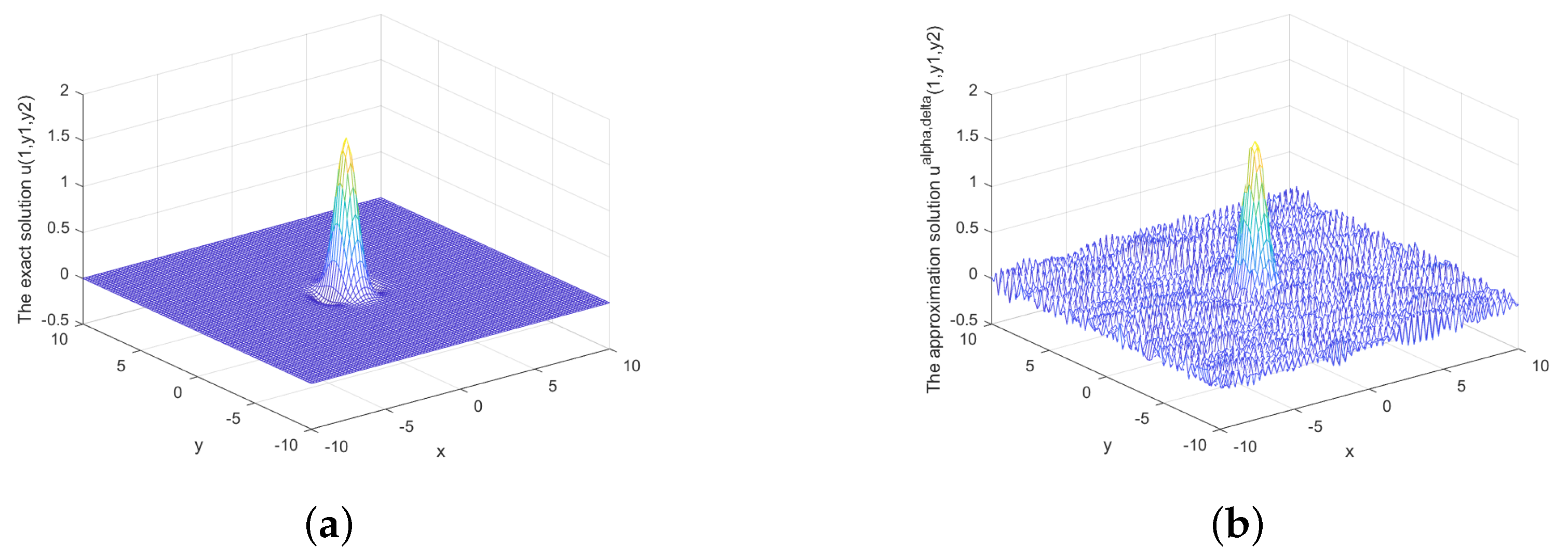
Figure 1, Figure 2, Figure 3, Figure 4 and Figure 5 are the comparison between the exact solution, approximate solution, and error under prior rule, from which we can see that our approach is stable and effective.

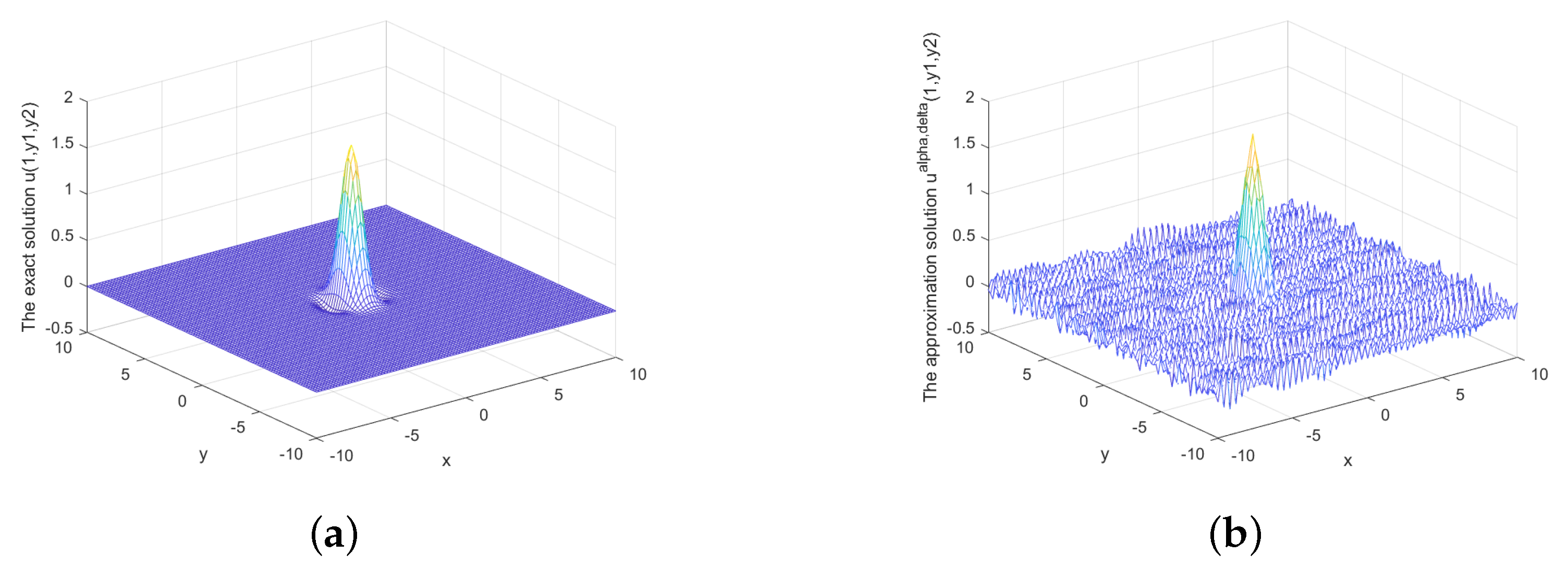
Figure 6, Figure 7, Figure 8, Figure 9, Figure 10 and Figure 11 are the comparison between the exact solution, approximate solution, and error under the posterior rule. The figure shows that our approach is also stable and effective under the posterior rule.

Figure 1 depicts the exact solution and approximate solution for $x=0.2$, $\delta =1\times {10}^{-2}.$ Figure 2 and Figure 3 show the relationship between the approximate solution and error under different $\delta =1\times {10}^{-3},\delta =1\times {10}^{-4}.$ Figure 4 and Figure 5 show the relationship between the approximate solution and error when $x=0.5$$,\delta =1\times {10}^{-5},\delta =1\times {10}^{-6}.$

Figure 6 shows the exact solution and approximate solution when $x=0.2$ and $\delta =1\times {10}^{-2}.$ Figure 7 and Figure 8 show the relationship between the approximate solution and error under different $\delta =1\times {10}^{-3},\delta =1\times {10}^{-4}$. Figure 9, Figure 10 and Figure 11 show the relationship between the approximate solution and error when $x=0.5$, $\delta =1\times {10}^{-5},\delta =1\times {10}^{-7},\delta =1\times {10}^{-8}.$

Table 1 and Figure 1, Figure 2, Figure 3, Figure 4, Figure 5, Figure 6, Figure 7, Figure 8, Figure 9, Figure 10 and Figure 11 show that the findings of relative error $rel(u)$ depend not only on error level $\delta$, but also on x. Our findings are stable and effective under both the prior and posterior rule.

Example 2.

We take function $\phi (y,z)=e^{-\frac{36}{36+y^2}-\frac{36}{36+z^2}}$, as the exact data of problem (4).

From

Table 2. Comparison between different regular solutions at x = 1.

p	$\mathit{\delta }$	Dirichlet $\mathit{rel}(\mathit{u})$	Posterior $\mathit{rel}(\mathit{u})$	Prior $\mathit{rel}(\mathit{u})$
0.5	1 × ${10}^{-8}$	0.2404	5.9947 × ${10}^{-4}$	6.212 × ${10}^{-4}$
0.5	1 × ${10}^{-9}$	0.0509	5.6870 × ${10}^{-5}$	5.9805 × ${10}^{-5}$
3	1 × ${10}^{-6}$	0.2684	0.0619	0.0590
3	1 × ${10}^{-7}$	0.0905	0.0056	0.0057

, we can see our approach is better than the approach of the study [30] at $x=1.$ The relative error of our approach is smaller than that in reference [30], the approximate effect is better, and the approach is more stable. Table 2 also reveals that the approach in this study is stable for $p=0.5$ and $p=3$, respectively.

Figure 12, Figure 13 and Figure 14 show the relationship between the exact solution, approximate solution and error under the prior rule. Figure 12 reveals the exact solution and approximate solution when $x=0.3$ and $\delta =1\times {10}^{-4}.$ Figure 13 reveals the approximate solution and the error between the exact solution and the approximate solution when $x=0.3$ and $\delta =1\times {10}^{-5}.$ Figure 14 illustrates the approximate solution and the error between the approximate solution and the exact solution when $x=0.3$ and $\delta =1\times {10}^{-6}.$ The above figures show that our approach is stable and effective under the prior rule, and the error decreases as the value of $\delta$decreases.

Figure 15, Figure 16 and Figure 17 illustrate the relationship between the exact solution, approximate solution and error under a posterior rule. Figure 15 shows the exact and approximate solution when $x=0.3$ and $\delta =1\times {10}^{-4};$ Figure 16 shows the approximate solution and the error between the exact solution and the approximate solution when $x=0.3$ and $\delta =1\times {10}^{-5};$ and Figure 17 illustrates the approximate solution and the error between the approximate solution and the exact solution when $x=0.3$ and $\delta =1\times {10}^{-6}.$ As can be seen from the above figures, our approach is also stable and effective under the posterior rule, and the error reduces as $\delta$ reduces.

The above is a graphical representation of the exact solution, approximate solution, and the error analysis under the priori regularization parameter choice rule and posterior regularization parameter choice rule. The above figures show that our regularization approach is stable and effective under both the prior and posterior rule, whether in the interval $0<x<1$ or on the boundary $x=1.$

6. Conclusions

In this study, we suggest a novel regularization method based on the bilateral kernel, to solve a Cauchy problem for a multi-dimensional Laplace equation in the mixed boundary. The error estimates are given under the prior and posterior rule. The numerical examples above show that it is feasible to solve the Cauchy problem for the multi-dimensional Laplace equation in the mixed boundary. The stable approximate estimates are obtained. Numerical examples show the numerical stability of the proposed method. Furthermore, our approach is superior to the paper [30] and the accuracy of the procedure is quite acceptable.

References

1. Tikhonov, A.N.; Arsenin, V.Y. Solutions of Ill-Posed Problems; Winson: Washington, DC, USA, 1977; pp. 10–80. [Google Scholar]
2. Colli-Franzone, P.; Magenes, E. On the inverse potential problem of electrocardiology. Calcolo 1980, 10, 459–538. [Google Scholar]
3. Alessandrini, G. Stable determination of a crack from boundary measurements. Proc. R. Soc. Edinb. 1993, 123, 497–516. [Google Scholar] [CrossRef]
4. Hadamard, J. Lectures on the Cauchy Problem in Linear Partial Differential Equations; Yale University Press: New Haven, CT, USA, 1923. [Google Scholar]
5. Reinhardt, H.J.; Han, H.; Hào, D.N. Stability and regularization of a discrete approximation to the Cauchy problem for Laplace’s equation. SIAM J. Numer. Anal. 1999, 36, 890–905. [Google Scholar] [CrossRef]
6. Klibanov, M.V.; Santosa, F. A computational quasi-reversibility method for Cauchy problems for Laplace equation. SIAM J. Appl. 1991, 56, 1653–1675. [Google Scholar] [CrossRef]
7. Wang, W.F.; Wang, J.R. Wavelet solution to the three-Dimensional Cauchy problem for Laplace equation. J. Math. 2012, 36, 239–248. [Google Scholar]
8. Hào, D.N.; Lesnic, D. The Cauchy problem for Laplace’s equation via the conjugate gradient method. IMA J. Appl. Math. 2000, 65, 199–217. [Google Scholar] [CrossRef]
9. Xiong, X.T.; Fu, C.L. Central difference regularization method for the Cauchy problem of the Laplace’s equation. Appl. Math. Comput. 2006, 181, 675–684. [Google Scholar] [CrossRef]
10. Fu, C.L.; Li, H.F.; Qian, Z.; Xiong, X.T. Fourier regularization method for solving a Cauchy problem for the Laplace equation. Inverse Probl. Sci. Eng. 2008, 16, 159–169. [Google Scholar] [CrossRef]
11. Li, Z.P.; Fu, C.L. A mollification method for a Cauchy problem for the Laplace equation. Appl. Math. Comput. 2011, 217, 9209–9218. [Google Scholar] [CrossRef]
12. Ang, D.D.; Nghia, N.H.; Tam, N.C. Regularized solutions of a Cauchy Problem for Laplace Equation in an irregular layer: A three-dimensional model. Acta Math. Vietnam 1998, 23, 65–74. [Google Scholar]
13. Cheng, J.; Hon, Y.C.; Wei, T.; Yamamoto, M. Numerical computation of a Cauchy Problem for Laplace’s equation. ZAMM J. Appl. Math. Mech. 2001, 81, 665–674. [Google Scholar] [CrossRef]
14. Manselli, P.; Miller, K. Calculation of the surface temperature and heat flux on one side of a wall from measurements on the opposite side. Ann. Mat. Pura Appl. 1980, 123, 161–183. [Google Scholar] [CrossRef]
15. Murio, D.A. Numerical method for inverse transient heat conduction problems. Rev. Unión Matemática Argent. 1981, 30, 25–46. [Google Scholar]
16. Murio, D.A. On the estimation of the boundary temperature on a sphere from measurements at its center. J. Comput. Appl. Math. 1982, 8, 111–119. [Google Scholar] [CrossRef]
17. Hao, C.; Li, F.X.; Fu, C.L. A mollification regularization method for the Cauchy problem of an elliptic equation in a multi-dimensional case. Inverse Probl. Sci. Eng. 2010, 18, 971–982. [Google Scholar] [CrossRef]
18. Engl, H.W.; Hanke, M.; Neubauer, A. Regularization of Inverse Problems; Kluwer Academic: Dordrecht, The Netherlands, 1996; Volume 35, pp. 4915–4920. [Google Scholar]
19. Yang, F.; Fu, C.L.; Li, X.X. A mollification regularization method for identifying the time-dependent heat source problem. J. Eng. Math. 2016, 100, 67–80. [Google Scholar] [CrossRef]
20. Xiong, X.T.; Mao, D.L.; Cao, X.X. A mollification method for solving the Cauchy problem for the modified Helmholtz equation. J. Northwest Univ. (Nat. Sci.) 2018, 53, 1–7. [Google Scholar]
21. Ern, A.; Guermond, J.L. Mollification in strongly Lipschitz domains with application to continuous and discrete de Rham complexes. Comput. Methods Appl. Math. 2016, 16, 51–75. [Google Scholar] [CrossRef]
22. Hào, D.N. A mollification method for ill-posed problems. Numer. Math. 1994, 68, 469–506. [Google Scholar]
23. Hào, D.N. A mollification method for a Noncharacteristic Cauchy Problem for a Parabolic Equation. Math. Anal. Appl. 1996, 199, 873–909. [Google Scholar] [CrossRef]
24. Hào, D.N.; Hien, P.M.; Sahli, H. Stability results for a Cauchy problem for an elliptic equation. Inverse Probl. 2007, 23, 421–461. [Google Scholar] [CrossRef]
25. Kumar, H.K.; Jiwari, R. A hybrid approach based on Legendre wavelet for numerical simulation of Helmholtz equation with complex solution. Int. J. Comput. Math. 2022, 99, 2221–2236. [Google Scholar] [CrossRef]
26. Kumar, H.K.; Jiwari, R. A note on numerical solution of classical Darboux problem. Math. Methods Appl. Sci. 2021, 44, 12998–13007. [Google Scholar] [CrossRef]
27. Xiong, X.T.; Shi, W.X.; Fan, X.Y. Two mumerical methods for a Cauchy problem for modified Helmholtz equation. Appl. Math. Model. 2011, 35, 4951–4964. [Google Scholar] [CrossRef]
28. Engl, H.W.; Hanke, M.; Neubauer, A. Regularization of Inverse Problem; Kluwer Academic: Boston, MA, USA, 1996. [Google Scholar]
29. Kirsch, A. An Introduction to the Mathematical Theory of Inverse Problems; Springer: New York, NY, USA, 1996. [Google Scholar]
30. He, S.Q.; Feng, X.F. A numerical Approximation Method for the Inverse Problem of the Three-Dimensional Laplace Equation. Mathematics 2019, 7, 487. [Google Scholar] [CrossRef]
Figure 1. (a) The exact solution and (b) the regularized solution when x = 0.2 , δ = 1 × 10 2 under prior rule.
Mathematics 11 01855 g001
Figure 2. (a) The regularized solution and (b) error between regularized and exact solution when x = 0.2 , δ = 1 × 10 3 under prior rule.
Mathematics 11 01855 g002
Figure 3. (a) The regularized solution and (b) error when x = 0.2 , δ = 1 × 10 4 under prior rule.
Mathematics 11 01855 g003
Figure 4. (a) The exact solution and (b) the regularized solution when x = 0.5 , δ = 1 × 10 5 under prior rule.
Mathematics 11 01855 g004
Figure 5. (a) The regularized solution when x = 0.5 , δ = 1 × 10 6 , (b) The regularized solution when x = 0.5 , δ = 1 × 10 7 under prior rule.
Mathematics 11 01855 g005
Figure 6. (a) The exact solution and (b) the regularized solution when x = 0.2 , δ = 1 × 10 2 under the posterior rule.
Mathematics 11 01855 g006
Figure 7. (a) The regularized solution and (b) error between regularized and exact solution when x = 0.2 , δ = 1 × 10 3 under the posterior rule.
Mathematics 11 01855 g007
Figure 8. (a) The regularized solution and (b) error between regularized and exact solution when x = 0.2 , δ = 1 × 10 4 under the posterior rule.
Mathematics 11 01855 g008
Figure 9. (a) The regularized solution and (b) error between regularized and exact solution when x = 0.5 , δ = 1 × 10 5 under the posterior rule.
Mathematics 11 01855 g009
Figure 10. (a) The regularized solution and (b) error between regularized and exact solution when x = 0.5 , δ = 1 × 10 7 under the posterior rule.
Mathematics 11 01855 g010
Figure 11. (a) The regularized solution and (b) error between regularized and exact solution when x = 1 , δ = 0.5 × 10 8 under the posterior rule.
Mathematics 11 01855 g011
Figure 12. (a) The exact solution and (b) the regularized solution when x = 0.3 , δ = 1 × 10 4 under a priori rule.
Mathematics 11 01855 g012
Figure 13. (a) The regularized solution and (b) error between regularized and exact solution when x = 0.3 , δ = 1 × 10 5 under a priori rule.
Mathematics 11 01855 g013
Figure 14. (a) The regularized solution and (b) error between regularized and exact solution when x = 0.3 , δ = 1 × 10 6 under a priori rule.
Mathematics 11 01855 g014
Figure 15. (a) The exact solution and (b) the regularized solution when x = 0.3 , δ = 1 × 10 4 under posterior rule.
Mathematics 11 01855 g015
Figure 16. (a) The regularized solution and (b) error between regularized and exact solution when x = 0.3 , δ = 1 × 10 5 under posterior rule.
Mathematics 11 01855 g016
Figure 17. (a) The regularized solution and (b) error between regularized and exact solution when x = 0.3 , δ = 1 × 10 6 under posterior rule.
Mathematics 11 01855 g017