Article

Nonstationary Time Series Prediction Based on Deep Echo State Network Tuned by Bayesian Optimization

1
School of Artificial Intelligence, Beijing Technology and Business University, Beijing 100048, China
2
Beijing Laboratory for Intelligent Environmental Protection, Beijing Technology and Business University, Beijing 100048, China
*
Author to whom correspondence should be addressed.
Mathematics 2023, 11(6), 1503; https://doi.org/10.3390/math11061503
Submission received: 8 February 2023 / Revised: 13 March 2023 / Accepted: 17 March 2023 / Published: 20 March 2023
(This article belongs to the Special Issue Time Series Analysis)

Abstract

:
The predictions from time series data can help us sense development trends and make scientific decisions in advance. The commonly used forecasting methods with backpropagation consume a lot of computational resources. The deep echo state network (DeepESN) is an advanced prediction method with a deep neural network structure and training algorithm without backpropagation. In this paper, a Bayesian optimization algorithm (BOA) is proposed to optimize DeepESN to address the problem of increasing parameter scale. Firstly, the DeepESN was studied and constructed as the basic prediction model for the time series data. Secondly, the BOA was reconstructed, based on the DeepESN, for optimal parameter searching. The algorithm is proposed within the framework of the DeepESN. Thirdly, an experiment was conducted to verify the DeepESN with a BOA within three datasets: simulation data generated from computer programs, a real humidity dataset collected from Beijing, and a power load dataset obtained from America. Compared with the models of BP (backpropagation), LSTM (long short-term memory), GRU (gated recurrent unit), and ESN (echo state network), DeepESN obtained optimal results, which were 0.0719, 18.6707, and 764.5281 using RMSE evaluation. While getting better accuracy, the BOA optimization time was only 323.4 s, 563.2 s, and 9854 s for the three datasets. It is more efficient than grid search and grey wolf optimizer.

1. Introduction

Data and information have been significant resources for management and control within many domains. Time series data become vital because they can represent the historical and future trends of the systems and elements involved in the economy [1,2,3,4], agriculture [5,6], and air monitoring [7,8,9,10]. Advanced time series prediction can help us make rational decisions, avoid risks, and reduce losses—contributing significantly to social management, economic manufacturing, and human life. In the real world, time series data show complex characteristics because they are affected by many factors in different systems. The nonstationary and nonlinear characteristics have been a typical issue of time series analysis, making it difficult to predict using subjective and empiric knowledge [11].
The field of time series prediction focuses on various types of methods, including statistical methods [12,13] and machine learning methods [14,15,16,17], which can be classified into shallow and deep models. Statistical methods, such as the autoregressive (AR), moving average (MA), autoregressive moving average (ARMA), and autoregressive integrated moving average (ARIMA) models, find data patterns through mathematical inference. The statistical methods run well based on the exploration of the data patterns. The typical processing methods transform nonstationary data into stationary data. However, during the process of processing, the problem of data feature loss will make the data incomplete, which results in the data lacking original meaning and interpretability; this means that there will be corresponding errors, thus resulting in prediction uncertainty. These classical methods have significant errors and low prediction performance for unstable and nonstationary data, which may fail during nonstationary time series prediction. Deep learning was developed, which has more robust data feature extraction abilities and improved computer operation capabilities. The deep network structure can build the model with more vital learning ability. By finely adjusting the learning rate, the region with more substantial fluctuations in nonstationary time series can obtain better learning and more accurate model parameters. Therefore, deep networks have received much attention in research and application within time series prediction. Parts of machine learning methods apply to the regression of the time series modeling, including the support vector machine, the recurrent neural network (RNN), long short-term memory (LSTM), and the gated recurrent unit (GRU). They can construct the mapping relation of the time series trend. Various machine learning methods perform differently due to the time series type, method structure, and computing resource.
The decomposition method is a data processing method that can reduce data complexity by decomposing a nonstationary time series into multiple series of lower complexity. In recent years, many researchers have widely used decomposition methods for time series prediction [18,19,20]. The decomposition method will generate random terms in decomposition, and the degree of nonstationarity of the random terms remains high and difficult to predict. In addition, the decomposition method creates a separate model for each component, making the overall model architecturally complex. Therefore, networks with high prediction accuracy and simple model structures have been a hot topic for researchers.
Performance improvement in machine learning usually relies on increased network structure and computing resources. It is expected to be able to obtain high prediction precision with relatively simple networks. The echo state network (ESN) [21] is a recurrent neural network that does not need to update parameters through a backpropagation algorithm. The ESN completes system modeling through the matrix operation of internal weights, which does not require parameter tuning in an iterative process, and thus, consumes fewer resources. The DeepESN [22] deepens the reservoir structure of the ESN with more prosperous feature extraction capabilities, further improving the prediction performance. The DeepESN is suitable for various scenarios and widely used in multiple time series prediction tasks. However, the DeepESN model has a complex structure and numerous parameters, which weakens the original advantage of the ESN in terms of network structure and learning mechanisms. Therefore, the DeepESN should be optimized in view of redundant parameters and appropriate structures.
In this paper, the DeepESN is studied to predict nonstationary time series. Hyperparameter tuning in the machine learning model is generally considered a black-box optimization problem. During the tuning process, only the input and output of the model are seen. For machine learning, the choice of different hyperparameters has a crucial influence on the result. It is essential to determine the optimal values of hyperparameters. The heuristic optimization algorithm is a comprehensive way to adjust parameters. Some heuristic optimization algorithms have been proposed and applied to solve many parameter optimization problems [23,24,25,26,27]. However, most optimization algorithms require enough initial sample points, thus increasing the optimization cost, and the optimization efficiency is not exceptionally high. We noticed that the Bayesian optimization algorithm could fully use the previous evaluation information when selecting the next set of hyperparameters. This can reduce the number of attempts required to determine hyperparameters and improve the model’s estimation and generalization abilities. The optimization efficiency is higher than the heuristic optimization algorithms and grid search. Therefore, Bayesian optimization was chosen as the optimization method—an efficient optimization algorithm suitable for DeepESN. In the optimization method, the parameters of DeepESN are determined adaptively, which can reduce the parameter search time and maintain model precision.
The prediction model and optimization methods were verified using simulated and real time series data, which are the data from mixed signal oscilloscopes (MSO), humidity data collected from Beijing, and electric load data from American Electric Load Company. The datasets cover the simulation data based on typical mathematic signals, natural phenomena, and human social behavior. Our proposed model achieved the best prediction accuracy on several metrics when several models were compared. This paper is organized as follows. Section 2 introduces the related works on time series prediction. Section 3 presents the DeepESN and BOA. Section 4 displays the experiment and results. The method is discussed and concluded, finally, in Section 5.

2. Related Works

Nonstationary time series have high complexity. In recent years, time series forecasting methods have mainly included statistical and neural network methods. In addition, the echo state network and its deformed structure have increasingly been widely used in time series research. In this section, related research is introduced from three aspects. Then, using the method proposed in this article, the existing problems are analyzed.

2.1. Sample Entropy Method and Autocorrelation Functions

Sample entropy [28] is a method used to measure the fluctuation and complexity of time series. It measures the complexity of the time series by calculating the probability of generating new patterns in the signal. The greater the probability of a new model, the higher the complexity of the time series.
For a set of time series  { u ( i ) , i = 1 , , N } , construct a  m  dimensional vector:
X m ( i ) = { u ( i ) , u ( i + 1 ) , , u ( i + m 1 ) } , 1 i N m + 1
Define the maximum distance function  d   [ X m ( p ) , X m ( q ) ]  of the vectors  X m ( p )  and  X m ( q ) , which is recorded as the number that meets the condition  d   [ X m ( p ) , X m ( q ) ] r . Define  n x i m  as the number of  X m ( q )  that have a distance between  X m ( p )  and a vector  X m ( q )  within  r .
The sample entropy is:
S a m p E n ( m , r , N ) = ln i = 1 N m 1 n x i m + 1 i = 1 N m 1 n x i m
The fluctuation and complexity of the time series can be measured using the method of sample entropy. The sample entropy measures the distance between two sub-vectors in a reconstructed time series. If the distance between any two sub-vectors is relatively close, the fluctuation and complexity of the time series are relatively weak. On the contrary, if the short distances between two vectors are relatively small, the time series has strong fluctuation and complexity.
The sample entropy can be set as a time series fluctuation and complexity measurement index. A threshold value can be selected, and a model with high prediction ability should be built when the entropy of a dataset is over the threshold value. The prediction models can be deep networks, as introduced in the following subsection.
The autocorrelation function refers to the correlation between neighboring variables of the time series. Assuming that the observed value of the series is  x t , x t 1 , , x t k , after the order of k, the correlation degree is defined as:
γ k = E ( x t , x t + k ) E ( x t 2 ) = t = 1 n k ( x t x ¯ ) ( x t + k x ¯ ) t = 1 n k ( x t x ¯ ) 2
where  x ¯  represents the sample mean and  E  represents the expectation function. The value of  γ k  is between −1 and 1; the closer to 1, the higher the degree of autocorrelation.
The autocorrelation function is either trailing or truncated for a stationary time series. The trailing refers to the function slowly approaching 0 at a negative exponential rate as the lag value  k  becomes larger. The truncation refers to the autocorrelation function becoming 0 when the lag value  k  is a specific value, like a truncated tail. The autocorrelation function does not have trailing and truncated tails for nonstationary time series.
Figure 1 shows the graph of the three data autocorrelation functions that were used. Its autocorrelation function has no tail or truncation, so it can be seen that they are non-stationary time series.

2.2. Statistical Models and Classical Neural Networks

Statistical methods are the earliest time series modeling methods. The ARMA [29,30] combines AR and MA for the stationary time series. The AR model treats subsequent data as a linear combination of previous data, and the MA model introduces a sliding window that can dynamically respond to time series characteristics. ARMA combines the advantages of the AR and MA models, which use statistical methods to model historical data, are simple to train, and have a good effect on dealing with complex time series. The ARIMA [31,32] model adds a different process, based on ARMA, which improves the nonlinear modeling ability. Amini et al. [33] built an ARIMA model to predict the electric vehicle charging demand for stochastic power system operation. The GARCH model can accurately simulate the fluctuation change of time series variables, and Caiado et al. [34] constructed it on finance time series. These methods are computationally small but very limited in their applicability to tasks and scenarios.
The machine learning method can extract data features more effectively using the computer’s computing power, thus capturing features more effectively when establishing the model. The classical time series neural network prediction fits the data and builds the model using error backpropagation. BP is the most basic neural network model, which reduces the error by continuously adjusting the model parameters. With the development of theory, the network structure with a deeper structure has been developed and studied. The deep network can mine the dependence on historical data and further extract the change rule of data. The RNN [35] model considers the influence of historical information on the current moment’s data. The LSTM [36] is one of the most widely used networks, and it further optimizes problems, such as gradient disappearance and explosion, in RNN. The GRU [37,38,39] reduces the number of gate units in the network technology of the LSTM and reduces computing consumption while achieving similar precision. Machine learning methods have been used for many tasks. Xue et al. [40] used the ELM to predict finance time series. Simran et al. [41] used the butterfly optimization algorithm (BOA) to optimize the LSTM network, and they utilized the LSTM network model to predict electricity consumption. Limei et al. [42] applied dynamic sliding windows to LSTM networks for water flow prediction. Xu et al. [43] built a dual-scale deep belief network, to predict the demand volume of urban water, that outperforms the single statistical model.
A single model is incapable of handling high-complexity nonstationary data. Thus, the hybrid modeling method of multiple models has been developed. Qiao et al. [44] established a hybrid model based on wavelet transform and an improved deep learning algorithm to predict PM2.5. Bao et al. [45] constructed stacked autoencoders and an LSTM to predict financial time series. Hanhong et al. [46] proposed a hybrid neural network model based on TCN and GRU to predict the short-term electricity load. The integrated model takes advantage of the advantages of multiple models to build models separately, which improves the predictive ability [47].

2.3. Echo State Network

Statistical methods are relatively simple to model but have insufficient predictive power. The machine learning method requires many calculations and takes a long time. The integrated learning method makes the model structure more complicated, which is not conducive to updating the model. The ESN is considered the most effective method for training recurrent neural networks, which have the advantages of a simple training process and short time consumption [48].
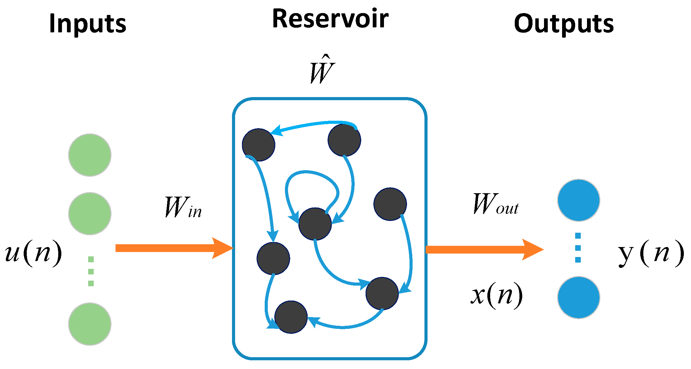
Figure 2 shows the structure diagram of the ESN. We define the  u ( n ) = [ u 1 ( n )   u k ( n ) ] T  as the input sample at time  n y ( n )  is the output corresponding to  u ( n ) . The input matrix  W i n  and the reservoir layer weight matrix  W ^  are uniformly distributed between −1 and 1, which remain fixed. To make the echo state network have echo properties, the spectral radius of the reservoir layer should be set between 0 and 1. During the training process, with the sample’s input, the reservoir layer’s state is updated using the following formula.
x ( n + 1 ) = f ( W i n u ( n + 1 ) + W ^ x ( n ) )
where  W i n  denotes the input connection matrix,  W ^  denotes the reservoir layer connection matrix, and  f  denotes the activation function inside the reservoir layer, which is usually taken strictly as a hyperbolic tangent function. According to the above state of the reservoir layer, the output of the ESN can be calculated using the following equation.
y ( n + 1 ) = f out ( W out x ( n + 1 ) )
where  W o u t  denotes the output connection matrix and  f o u t  denotes the output excitation function. During training, the reservoir layer states are collected into a state matrix X. The final network output weight  W o u t  can be calculated using the following equation.
W o u t = ( X T X ) 1 X T Y
where X denotes the matrix form of the input reservoir state and Y denotes the output matrix form. The superscript  T  represents the matrix transpose and  1  represents the inverse of the matrix. The optimal solution of the output matrix can be found using least squares or MSE alone. Since the output function is a standard linear function, Equation (6) can be derived from the loss function  L = | W o u t X Y | , where  L  denotes the loss matrix.
Researchers have implemented some optimizations and improvements to the structure of the ESN, such as the quantum echo state network [49] and the robust echo state network [50], and the DeepESN [22] is a neural network composed of multiple reservoirs. It has excellent predictive capabilities and has been applied to various tasks. It has been a research hotspot in recent years, and we will study it in this paper. The DeepESN has many network parameters, so it is difficult to determine a suitable network structure. Therefore, we propose the BOA to optimize the DeepESN, which can adaptively determine the network model structure within a limited amount of time, thus saving network modeling time and making the network more suitable for various tasks [51,52,53,54,55,56,57].
Significantly different from previous studies, we propose a DeepESN optimized by the BOA for predicting complex time series. Our innovative contributions are highlighted as follows:
(1)
The BOA is used to optimize the DeepESN so that the network parameters are easily set and the final model is easier to determine.
(2)
Bayesian optimization is applied to nonstationary time series prediction, and excellent prediction results are obtained.

3. Bayesian Optimization of Deep Echo State Network

3.1. Deep Echo State Network

The DeepESN is a novel deep network structure that replaces a single reservoir layer with an ESN with multiple reservoir layers. It consists of an input layer, a multiple-reservoir layer, and an output layer. The input layer feeds data into the entire network. The reservoir layers process and compute the data to obtain the internal state. The output layer fits the internal states to the actual values to obtain the model parameters. Compared with the backpropagation algorithm, the DeepESN only requires matrix operations and does not require many backpropagation iterations. Further, the DeepESN has a more robust feature extraction ability and better prediction accuracy than a simple ESN.
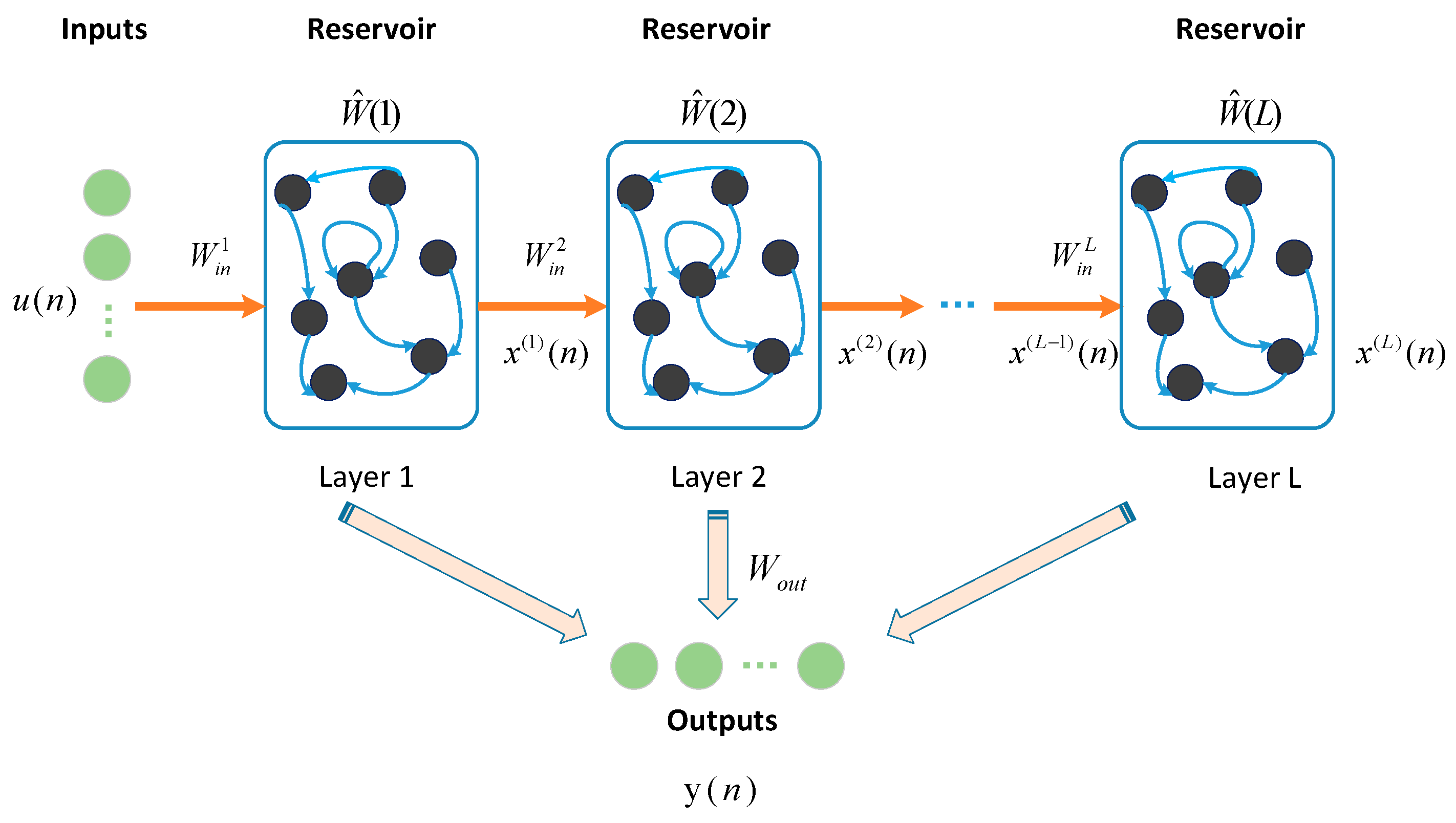
Figure 3 shows the structure of the DeepESN. We define  u ( n ) = [ u 1 ( n )   u k ( n ) ] T  as the input sample at time  n . After each sample is inputted into the DeepESN network, the state of the reservoir layers in the DeepESN will be updated. For the state of the  l  reservoir layer, it is updated using the following formula:
x ( l ) ( n ) = ( 1 a ( l ) ) x ( l ) ( n 1 ) + a ( l ) tanh ( W i n ( l ) i ( l ) ( n ) + θ ( l ) + W ^ ( l ) x ( l ) ( n 1 ) )
i ( l ) ( n ) = { u ( n ) , l = 1 x ( l 1 ) ( n ) , l > 1
where  x ( l ) ( n )  represents the state obtained by the reserved layer  l  when the first sample is inputted.  a ( l )  represents the leaking rate of the layer  l tanh  is the hyperbolic tangent activation function,  W i n ( l )  represents the input matrix of the input layer,  W ^ ( l )  represents the internal matrix of the reservoir layer, and  W i n ( l )  and  W ^ ( l )  are the fixed parameters.  i ( l ) ( n )  represents the input of the reservoir layer. When  l  is 1, the input of the reservoir layer is the original sample; when  l  is greater than 1, the input layer of the reservoir layer is the state of the reservoir layer.
Finally, the state of each reservoir layer is collected to get the state of the entire network.
x ( n ) = [ x ( 1 ) ( n ) x ( 2 ) ( n ) x ( l ) ( n ) ] T
The output weight and the state collected by the network will be multiplied by the matrix to get the final network output value.
y ( n ) = g ( W o u t x ( n ) )
The output weights  W o u t  are the model parameters that need to be calculated by the network. The  W o u t  is the parameter that only needs to be trained. Sort all  x ( n )  and  y ( n )  by row to get  X  and  Y , the final model parameters.  W o u t  can be calculated using the following formula:
W o u t = Y X T ( X X T + α E ) 1
where  α  is the regularization coefficient,  E  is the unit matrix, the superscript  T  represents the matrix transpose, and  1  represents the inverse of the matrix. The derivation principle of Equation (11) is similar to that of Equation (6) and can be derived from the loss function  L = | W o u t X Y | + α W o u t , where  L  denotes the loss matrix.

3.2. Bayesian Optimization Algorithm

The BOA is an effective hyperparameter optimization algorithm. It can find the best model parameters faster than a grid and random search. Each parameter is in a specific interval, and all parameters constitute a hyperparameter space. For different hyperparameter combinations, the prediction performance of the model is different. The model’s accuracy gets higher and higher through the optimization process, and the predicted result is closer to the actual value. The objective optimization function can be expressed as:
f ( x ) = i = 1 n u m ( y ( x i ) y ^ i ) 2 n u m
where  y ^ i  is the true value and  y ( x i )  is the predicted value.  n u m  is the length of the input time series. The optimal parameters can be obtained through the BOA, which makes the optimized target reach the minimum value.
The objective function of the BOA can be simplified as:
x = a r g m i n x X f ( x )
where  X  stands for parameter combination,  x  represents the best parameters obtained, and  x  is a group of hyperparameter combinations.
The BOA finds new evaluation points by maximizing the acquisition function to weigh the distribution of evaluation points and the improvement of prediction performance; it then re-imports them as inputs in the model to obtain new outputs so that it can continuously update and find model parameters. We chose the Gaussian function as the distribution hypothesis of the prior function and then used the acquisition function to select the next point in the posterior process for evaluation. The Gaussian process (GP) is an extension of the multidimensional Gaussian distribution, which can be defined using mean and covariance. The covariance function of a GP is its kernel function  k ( x , x ) . The kernel function measures the role of the distance between any two points,  x  and  x .
f ( x ) G P ( μ ( x ) , k ( x , x ) )
μ ( x ) = E [ f ( x ) ]
k ( x , x ) = E [ ( f ( x ) μ ( x ) ) ( f ( x ) μ ( x ) ) ]
Usually, the mean function is set to zero; then, the above Gaussian process can be expressed as:
K n = ( k ( x 1 , x 1 ) k ( x 1 , x n ) k ( x n , x 1 ) k ( x n , x n ) )
When a new set of evaluation samples are added to the set of all evaluation points, the covariance matrix formula is updated to:
{ K n + 1 = ( K n k n T k n k ( x n + 1 , x n + 1 ) ) k n = [ k ( x n + 1 , x 1 ) , k ( x n + 1 , x 2 ) , , k ( x n + 1 , x n ) ]
Using the updated covariance matrix, we can get the posterior probability:
P ( f n + 1 | D n + 1 , x n + 1 ) N ( μ n + 1 ( x ) , σ n + 1 2 ( x ) )
where  D  is the observation data,  μ i + 1 ( x )  is the mean value of  f ( x )  at step  i + 1 , and  σ i + 1 2 ( x )  is the variance of  f ( x )  at step  i + 1 .
The value of the function can be sampled from the joint posterior distribution by evaluating the mean value and covariance matrix. The sampling function can determine the next point to be evaluated to find the optimal parameter value faster and reduce resource consumption. We choose the UCB function as the sampling function, and the expression is as follows:
x i + 1 = arg max H ( x | D i ) = arg max μ ( x ) + ζ i + 1 1 2 σ i ( x )
where  ζ i + 1 1 2  is a constant,  H ( x | D i )  is the UCB acquisition function, and  x i + 1  is the selected hyperparameter of step  i + 1 .
In this paper, we optimized five important parameters of the DeepESN: layers, number of neurons, leaking rate, spectral radius rate, and input scaling. Among them, the spectral radius is the maximum value of all of the eigenvalues of the reservoir weights, and it is the main factor affecting the memory capacity of the reserve. It is necessary to make the spectral radius less than 1 to ensure the convergence of the network. Input scaling is the pre-processing data method used to limit the range of input data. The entire algorithm flow is shown in Algorithm 1.
Algorithm 1: DeepESN optimized by the BOA.
Input: Select the parameters to be optimized in the DeepESN model and determine the optimization space  X . Set the number of iterations of the BOA as  n .
Output: returns the optimal hyperparameter group  x .
For i = 1: n
    Select a set of optimized parameters  x  from  X .
    Train the DeepESN model with parameters  x .
    Evaluate model prediction performance using Equation (11).
    Update the covariance matrix and get the posterior probability.
    Based on the current results, obtain the next set of model parameters.
Evaluate the model using Equation (12) and obtain the optimal model parameters  x .

4. Experiment and Results

4.1. Experimental Setup

The data used in the experiments included two types of data, which were simulation data and actual data. The simulation data were obtained through computer simulation, and the real data were collected from the actual generation. The MSO dataset, obtained through computer simulation, was used as the simulation data. The actual data were the collected humidity data from the meteorological field and the electric load data from the electric power industry. The sample entropy was calculated for the three datasets according to the method in Section 2.1, and the results are shown in Table 1.
For each dataset, four value intervals were selected as 0–500, 500–1000, 1000–1500, 1500–2000. The sample entropy was calculated for these four intervals, and Table 1 shows the specific results. It can be seen that the sample entropy was large, and the magnitude of the sample entropy varied widely between segments, implying a high level of fluctuation and complexity within the dataset. This shows that the models of high prediction ability should be applied to the time series.
The experimental platform of this paper was based on 64-bit Windows. The RAM was 8 GB, and the core was i7-8565u at 1.8 GHz. The deep learning framework used the Tensorflow interface of Keras, the optimizer was Adam, and the code was executed in python.
In the experiments in this paper, several typical models were chosen to compare with the Bayesian-optimized DeepESN to demonstrate the superior predictive power of the model. The typical models of the backpropagation neural network and the primary echo state network were chosen as the comparison models. Among them, the BP model used for comparison is the most classic neural network model and the most basic method used for non-stationary time series forecasting. The LSTM is a deep learning model method that has achieved good results in many time series forecasting tasks. The GRU is the optimized structure of the LSTM and is also used as a comparison model. These backpropagation models were used for comparison with the deep echo state networks to illustrate the learning ability of non-backpropagation networks and prove that deep echo state networks have good accuracy while consuming fewer resources. The ESN was used as the basic model, and the DeepESN was used for comparison in regard to prediction performance, thus confirming deep networks’ superiority in prediction accuracy. Therefore, we chose the above model as the comparison model.
To verify the efficiency of the BOA in parameter search, we compared the Bayesian optimization with the grid search method and the grey wolf optimizer (GWO) [26]. Too many grid search cases for five parameters would consume significant computational time. Therefore, we selected four values at equal intervals instead of the original parameter interval for each parameter. Thus, with four cases per parameter, the total number of parameter selection cases, by grid search for five parameters, was 1024. The GWO used 10 initial sample points and iterated 50 times.
In the field of time series forecasting, there are many indicators used to evaluate the forecasting effect. In this paper, we chose RMSE, MAE, R2, and CC as the evaluation indexes. RMSE and MAE can most directly measure the forecasting effect. The smaller their values, the more accurate the prediction. R2 and CC measure the linear relationship between predicted and true values. The closer the value is to 1, the stronger the linear relationship between the predicted and true values. In addition to the calculated value of the CC, it is also necessary to check its significance level, represented by the P-value. Generally, when the P-value is less than 0.05, it can indicate a significant correlation between the two data groups, and chance factors do not cause the CC value. The P-values of the three data groups were 0.000492, 3.212 × 10⁻¹³, and 6.338 × 10⁻¹¹, which meant that the datasets were significantly correlated and their evaluation indicators for CC were reliable.
R M S E = 1 T i = 1 T ( y r y p ) 2
M A E = i = 1 T | y r y p | T
R 2 = 1 i = 1 T ( y p y r ) 2 i = 1 T ( y p y r v ) 2
C C = i = 1 T [ y r ( i ) y r v ( i ) ] [ y p ( i ) y p v ( i ) ] i = 1 T [ y r ( i ) y r v ( i ) ] 2 i = 1 T [ y p ( i ) y p v ( i ) ] 2
where  y r  represents the real value,  y p  represents the predicted value,  T  represents the number of data,  y r v  represents the average value of the real value, and  y p v  represents the average value of the predicted value.

4.2. Datasets

MSO simulation data is a typical nonstationary time series. It consists of several sinusoidal components of different frequencies superimposed on each other. The following formula can represent it:
y ( n ) = i = 1 s sin ( α i n )
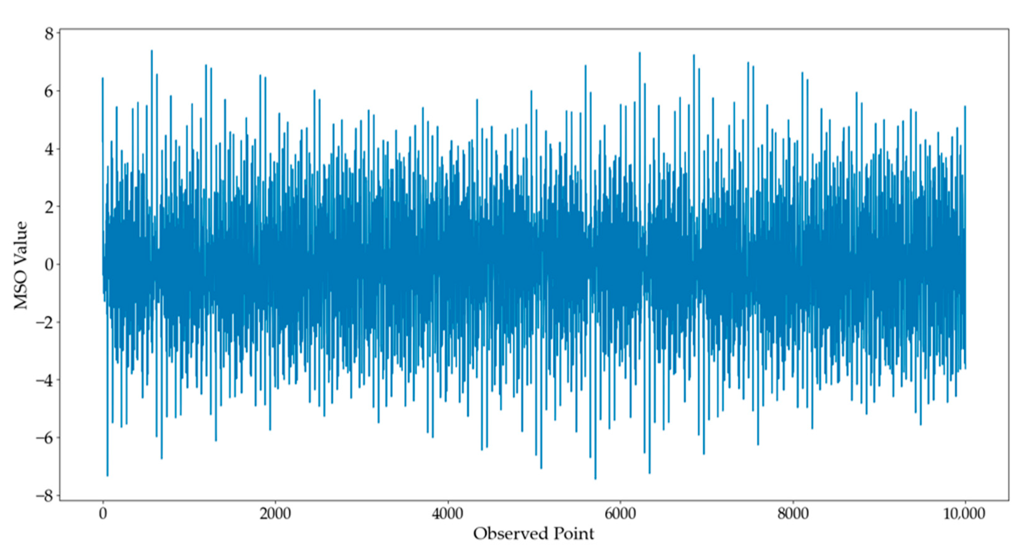
where  s  represents the number of sinusoidal frequencies,  α i  represents the frequency of the ith component, and  y ( n )  represents the n-th sample. In our experiment, we selected MSO data composed of 8 frequencies. The frequency components were:  α 1 = 0.2 α 2 = 0.311 α 3 = 0.42 α 4 = 0.51 α 5 = 0.63 α 6 = 0.74 α 7 = 0.85 α 8 = 0.97 . The MSO data are shown in Figure 4. The first 80% of the data was used as the training set, and the last 20% was used as the test set.
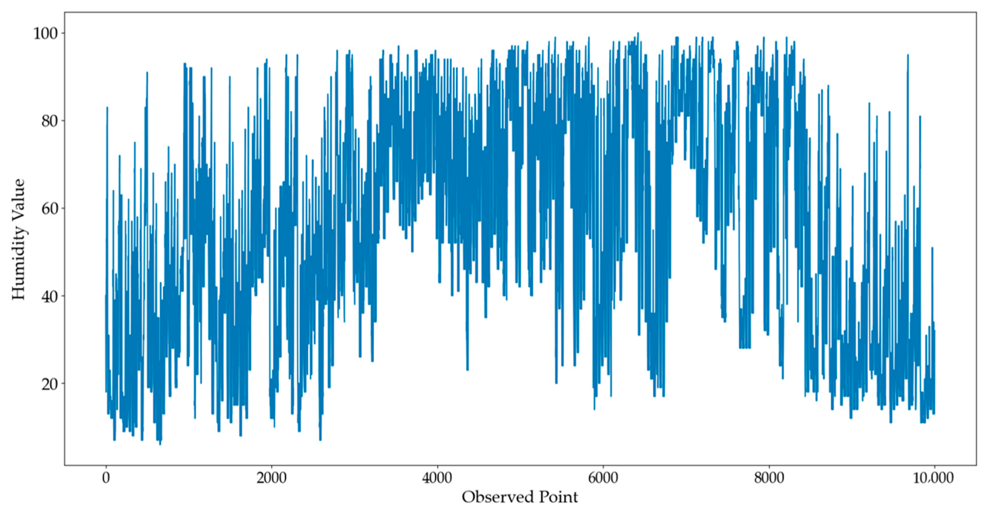
The data on humidity are recorded every hour in Beijing, China. The data of 7680 h across 320 days were set as the training data, and data of 1920 h across the next 80 days were the test data. In this experiment, a 24-step was set as the forward prediction length. The original humidity data are shown in Figure 5.
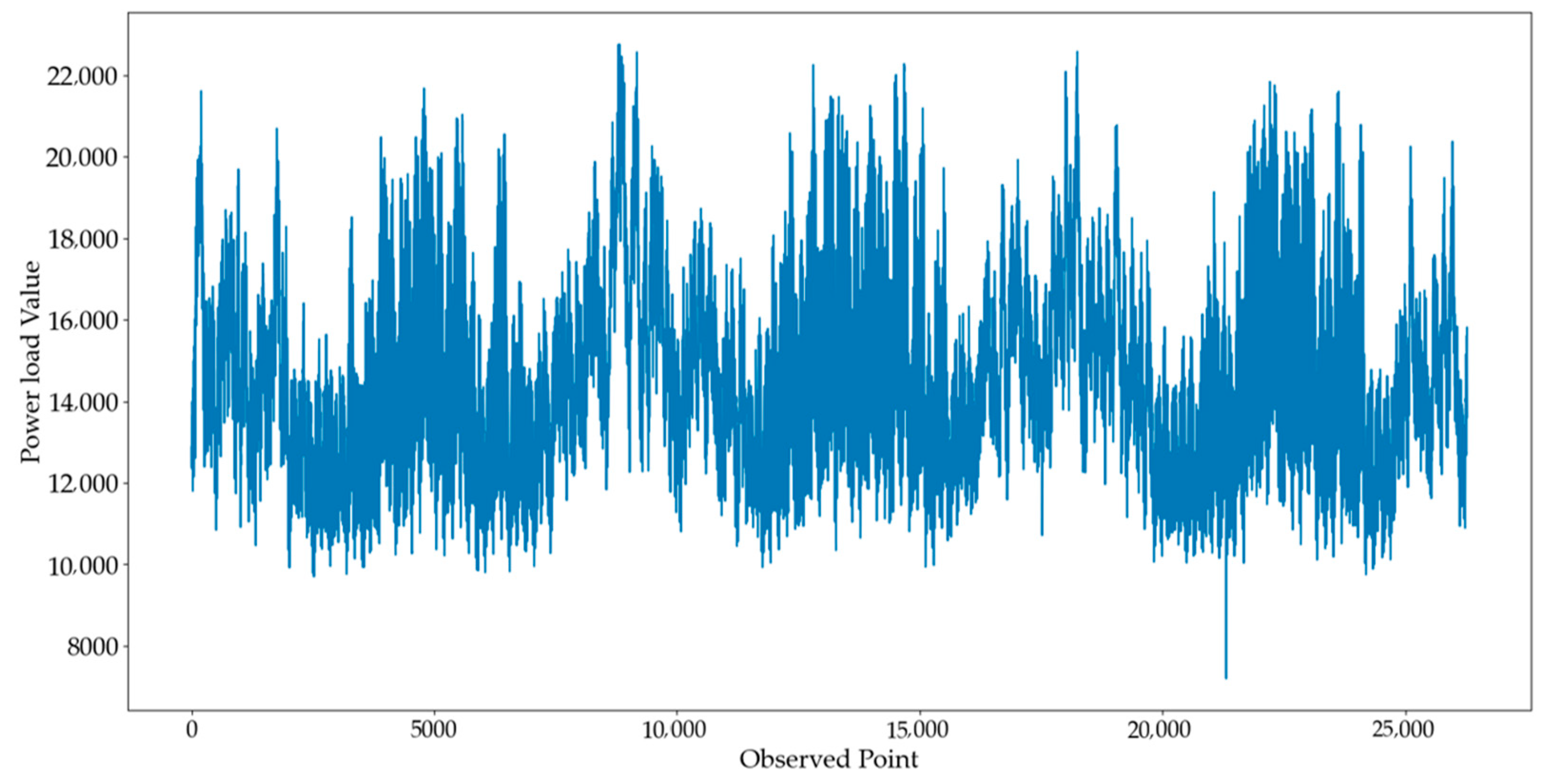
Power load data has strong non-stationarity due to the influence of season and temperature. We collected electricity data from the American Electric Load Company from 1 January 2017 to 1 January 2020. The data were collected every hour, for a total of 26,280 h. In our research, we selected the first 500 days of data, a total of 12,000 h, as the dataset. The first 80% of the data was used as the training set, and the last 20% was used as the test set. Figure 6 shows the original power load data.
The datasets are also presented with the statistical indicators in Table 2. The statistics include the minimum, maximum, mean, standard deviation, and variance. Figure 4, Figure 5 and Figure 6 and Table 2 show the datasets have complex trends in different scales. When performing the Bayesian optimization of the DeepESN, the parameters to be optimized differed for each dataset, depending on the data type and size. For the above three datasets, we set the parameter ranges as Table 3. For the comparison networks, the relevant parameters are shown in Table 4. In particular, the comparison networks were optimized using the grid searching method. This guaranteed that the prediction results of the BP, LSTM, GRU, and ESN had reached the best level of the experimental data.

4.3. Results

4.3.1. Results for the MSO Data

Figure 7 shows the prediction results of each model for the MSO simulation data, which are represented by curves of different colors. It can be seen from the figure that the Bayesian-optimized DeepESN, represented by the purple curve, is closest to the true value among all the models.
To intuitively display the predicted results of each model, the above evaluation indexes were used to calculate the experimental results. The specific results are shown in Table 5. The bold in Table 5 represents the model proposed in this paper and the best results in the evaluation indexes.
It can be seen that the DeepESN achieved optimal values for RMSE, MAE, CC, and R2. Compared with the neural network algorithm, the prediction ability of the DeepESN has a significant advantage. Meanwhile, the prediction performance is improved based on the ESN. This experiment verifies the prediction ability of the DeepESN on simulated datasets.
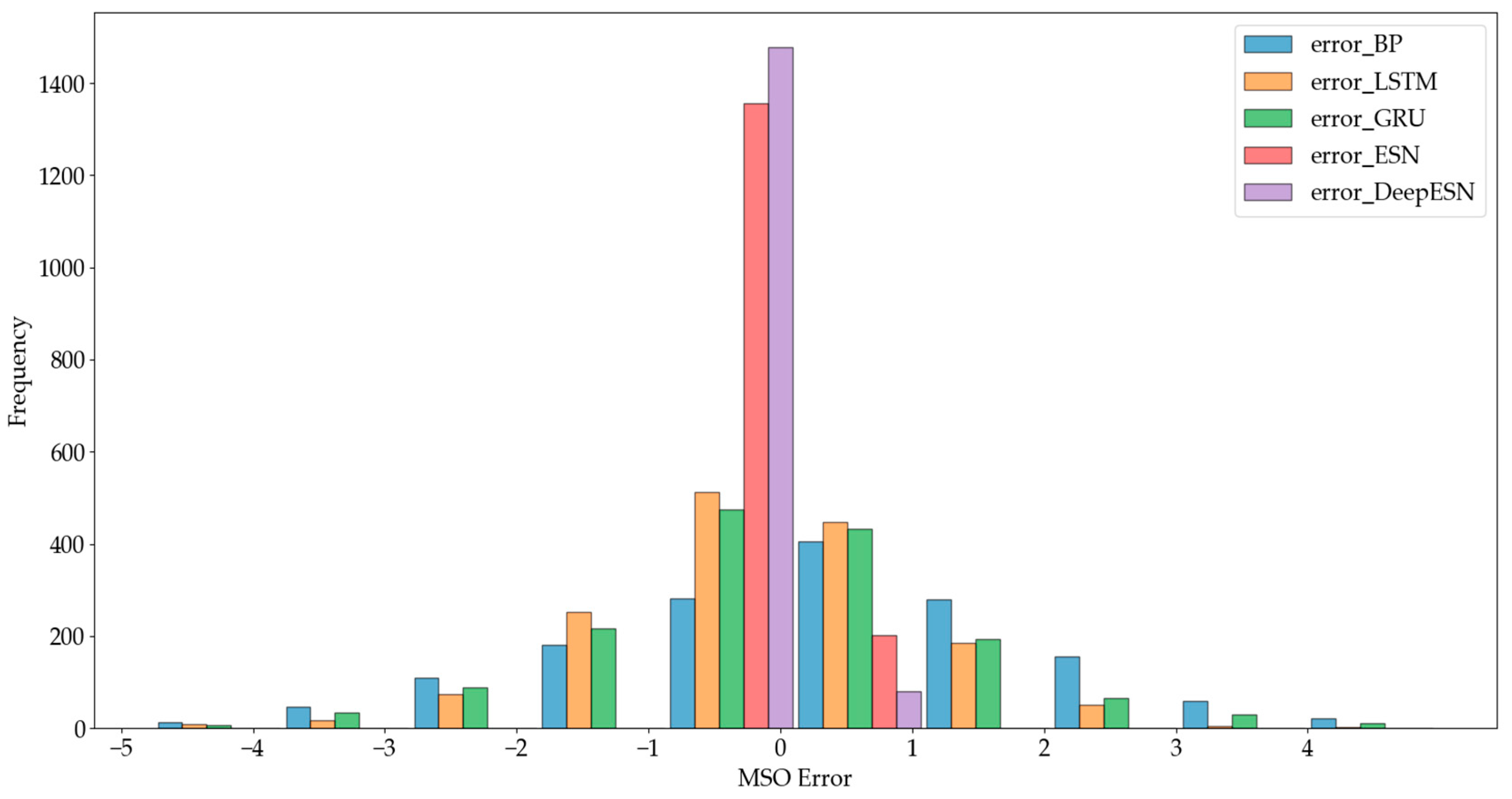
Figure 8 shows the histogram of the prediction errors of different models on the MSO dataset. The minimum value of the errors was −4.7455, and the maximum was 4.9751. The errors were divided uniformly into 10 intervals. The prediction errors of the DeepESN, indicated in purple, were concentrated in the interval closest to [−0.85726, 0.1148]. Compared to other models, the overall errors of the DeepESN were the smallest, and the best prediction results were obtained.

4.3.2. Result of Humidity Data

Figure 9 shows the prediction results of each model on the actual humidity data. It can be seen from the figure that the Bayesian optimization DeepESN, represented by the purple curve, was the closest to the true value among all the models.
The results of the evaluation metrics calculations are shown in Table 6. The bold in Table 6 represents the model of this paper and the best results. The results show that the DeepESN model had the smallest RMSE, the smallest MAE, the largest R2, and the largest CC. The DeepESN model had fewer errors and more accurate predicted values than the other models.
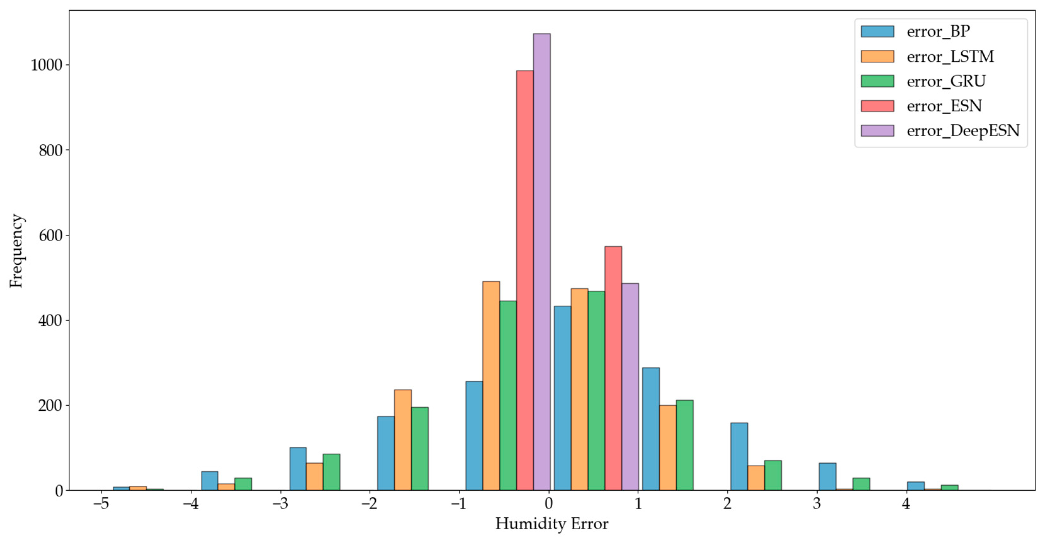
The histogram of prediction errors is shown in Figure 10. For the different models, the minimum value of the errors was −4.8994, and the maximum was 4.9751. The error distribution shows that the DeepESN, indicated in purple, was concentrated at [−0.9496, 0.03789]. The errors of the other models were located in intervals of big values.

4.3.3. Result of Power Load Data

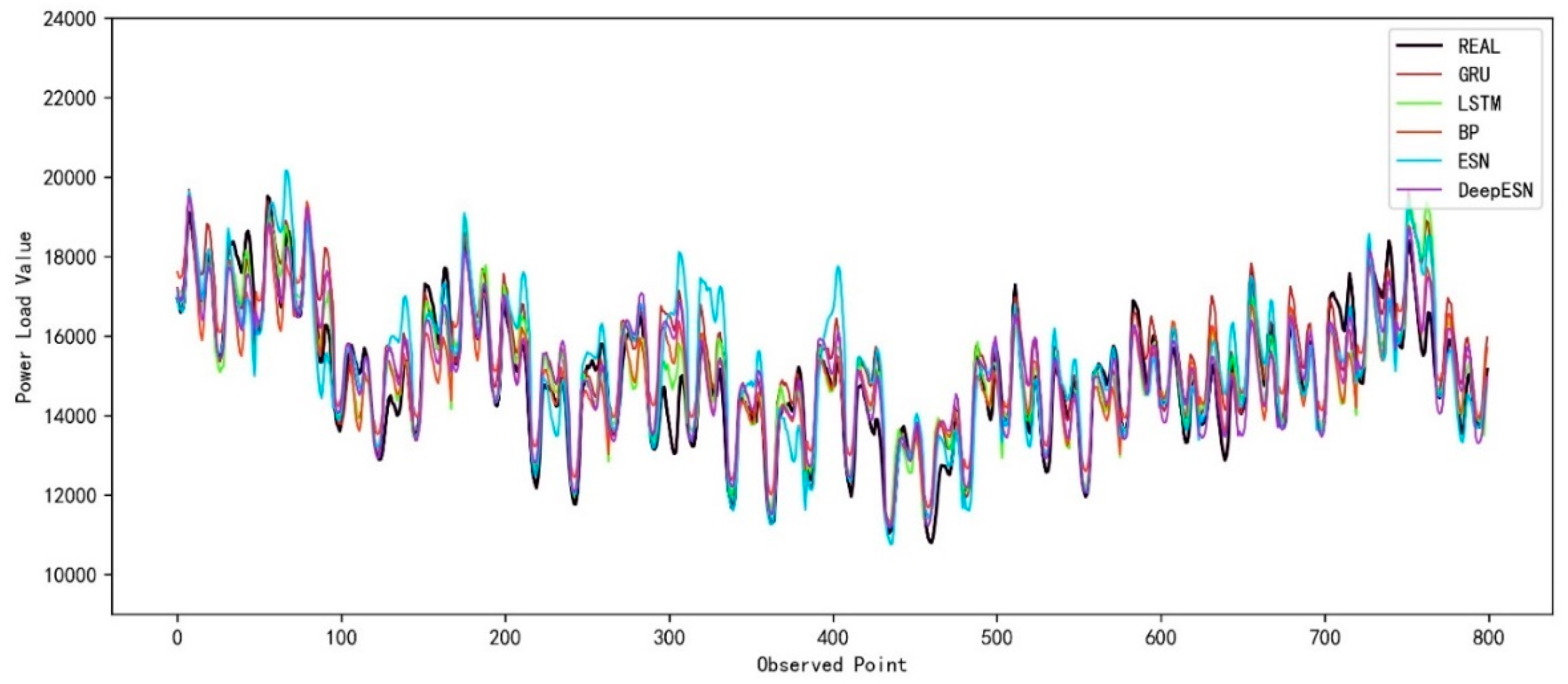
Figure 11 shows the prediction results of each model on the actual power load data. Compared with the other curves, the DeepESN, represented by the purple curve, was the closest to the true value.
The results of the evaluation metrics calculation are shown in Table 7. The bold in Table 7 represents the model selected in this paper and the optimal eval-ua-tion index, respectively. As with the prediction results of the humidity dataset, the DeepESN model had the smallest RMSE and MAE and the largest R2 and CC for the power load dataset, which confirms the prediction ability of the DeepESN for the actual dataset.
Through the above three groups of experiments and comparisons of the prediction curves and several evaluation indexes, it can be concluded that the Bayesian-optimized DeepESN has good prediction performance. Compared with other models, the DeepESN achieved better prediction results on both the simulated and real datasets, which confirms the advantages of the DeepESN in nonstationary time series prediction.
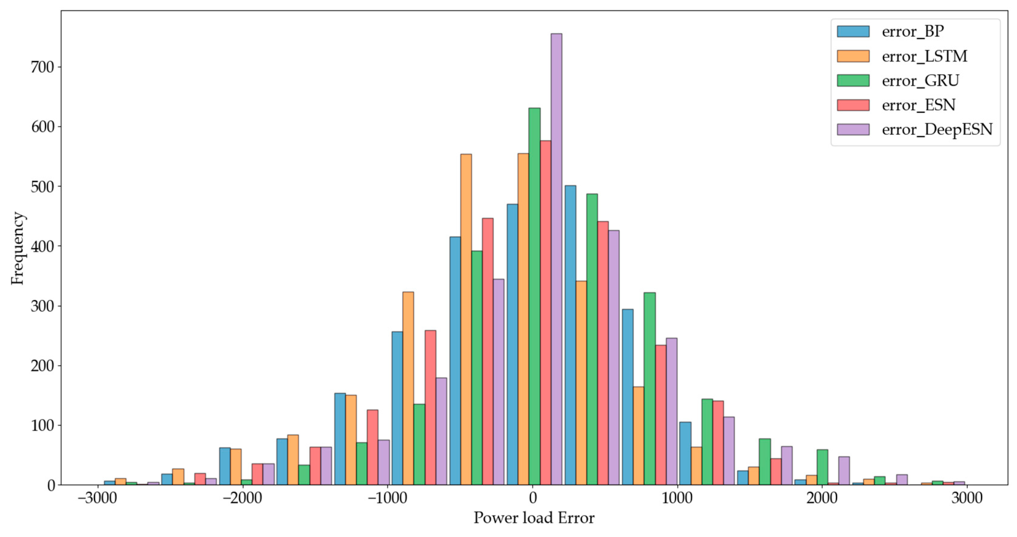
Figure 12 shows the histogram of prediction errors for the power load dataset. The data of power loads is complicated to predict. The minimum error value was −2968.06, and the maximum was 2993.299. The errors were divided into 15 intervals. The prediction errors of the DeepESN, indicated in purple, were concentrated at [−186.0927, 211.3312]. The Gaussian distribution of the errors showed that the DeepESN obtained the best prediction results.

4.3.4. Result of Bayesian Optimization Algorithm

Grid search and GWO were performed on the same dataset, and the optimization results were compared with the BOA method. Table 8 compares the experimental results of the three optimization methods for the three datasets.
Table 8 shows the metrics of the three optimization methods on the three datasets. By comparison, it was found that the BOA obtained the best results across four prediction accuracy metrics while consuming the least amount of time. Compared with grid search and GWO, the BOA can obtain better prediction results in the shortest time
Table 9 shows the parameters finally selected by the DeepESN for the three experiments by the three optimization methods.
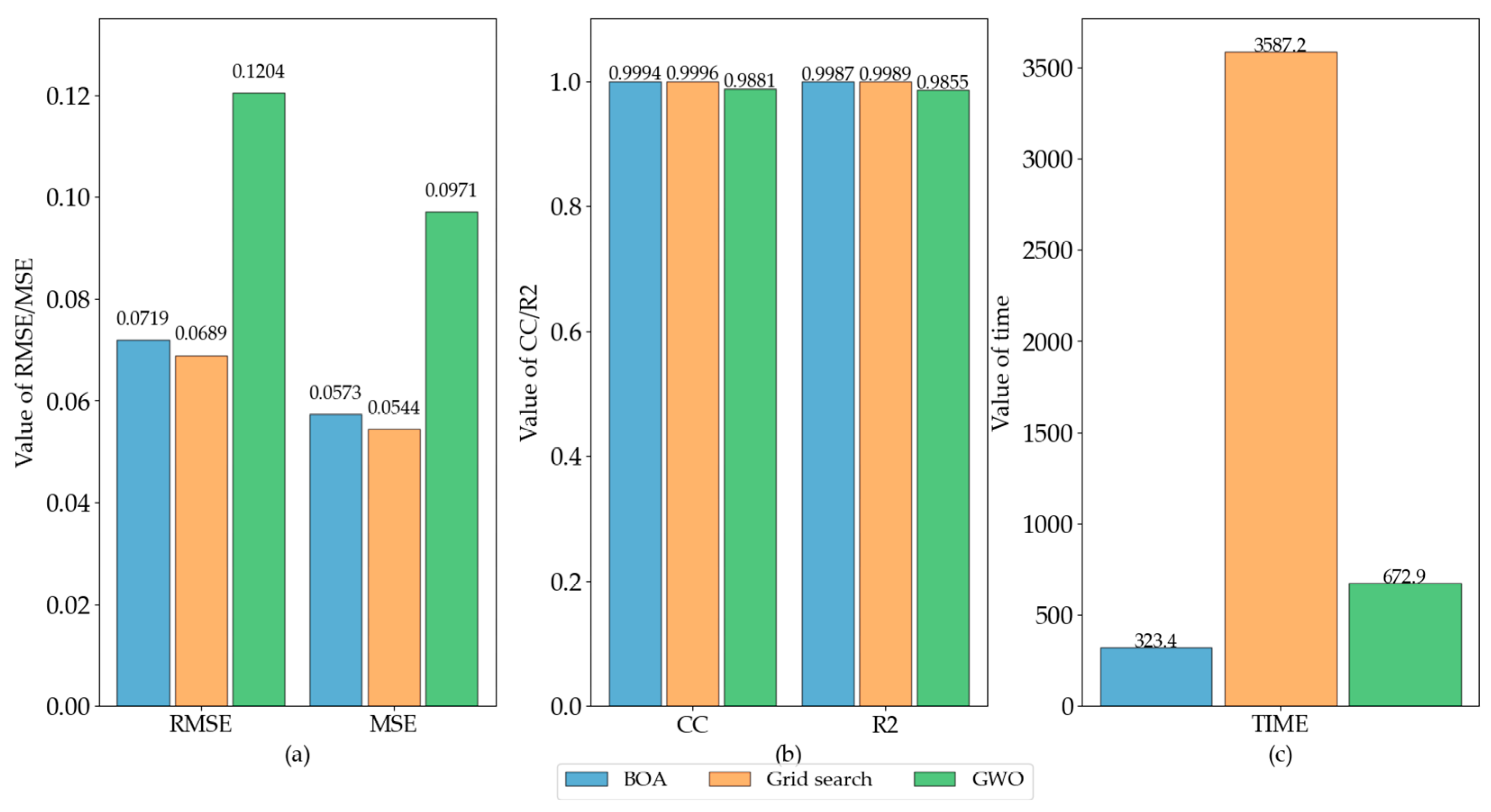
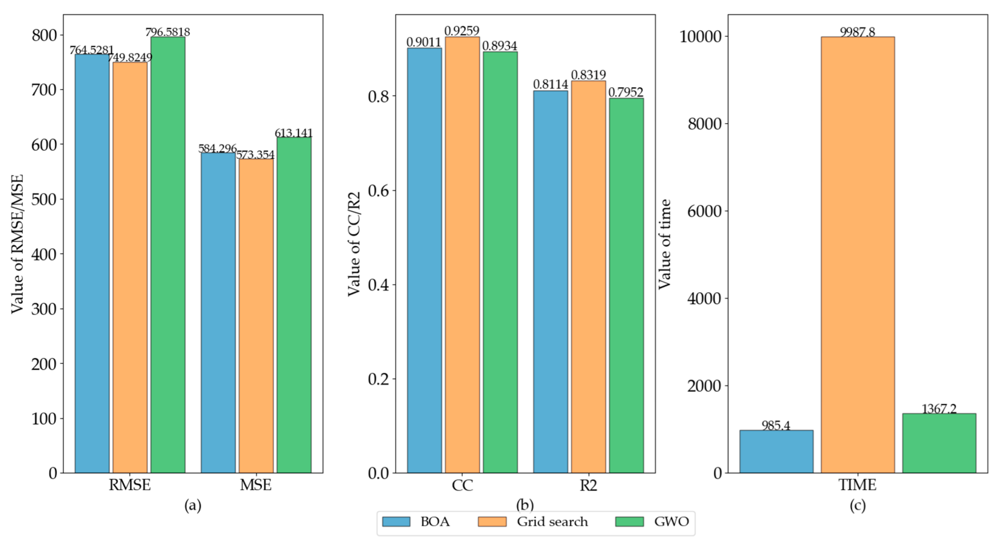
For a more visual comparison of the results, we plotted the comparison of the evaluation results of different optimization approaches for each dataset using bar charts. Evaluation indicators included RMSE, MAE, R2, CC, and consumption time. Figure 13, Figure 14 and Figure 15 show each dataset’s evaluation indicators for different optimization methods. In the figures, subplot (a) shows the comparison of RMSE and MSE, subplot (b) shows the CC and R2, and subplot (c) shows the comparison of running time.
As shown in Figure 13, the simulation data MSO, BOA, and grid search achieved extremely close results in the evaluation indicators, indicating that the two optimization methods can achieve close results, while GWO had poor prediction results. Regarding time consumption, The BOA method consumed less time, followed by GWO and grid search, which indicates that the BOA method is efficient in parameter search.
Figure 14 shows that the BOA and grid search optimization methods had the highest prediction accuracy for the humidity data. Moreover, the time consumed by the BOA was relatively lower among the three optimization algorithms.
As shown in Figure 15, similar to the results in the MSO and humidity datasets, the BOA can achieve similar prediction accuracy to a grid search in power load experiments, and it has the shortest optimization time compared with grid search and GWO.
In three experiments comparing the results of three experiments by three different optimization methods, the results of the BOA were close to the grid search for multiple indicators of RMSE, MAE, CC, and R2. However, the results predicted using the GWO method were relatively poor. Meanwhile, in these three cases, the BOA method consumed the least time of all three cases, which means that fewer computational resources were used, showing the efficiency of the BOA in the parameter search task. It is confirmed that the Bayesian optimization method is an effective way to optimize the DeepESN.

5. Discussion and Conclusions

This paper used the Bayesian-optimized DeepESN to model and predict simulated and real data. The prediction results showed that, compared to ARIMA, BP, LSTM, GRU, and ESN networks, the Bayesian-optimized DeepESN was closer to the curve the actual values represented. The evaluation metrics showed that the Bayesian-optimized DeepESN achieved the best prediction results across several evaluation metrics compared to other network types.
Experiments were conducted to compare the BOA, grid search methods, and GWO to optimize the DeepESN in three ways. The BOA can use previous validation results to reasonably collect the parameters for the next time. With almost the same prediction accuracy, the BOA significantly reduces the parameter search time, decreases time complexity, and proves that the BOA has a very efficient effect in performing the parameter optimization of the model. Therefore, the Bayesian-optimized DeepESN can significantly reduce the model tuning time, improve the prediction accuracy and reduce resource consumption.
Compared with echo state networks, the DeepESN has richer dynamic characteristics, stronger short-term memory storage capacity, and more accurate temporal prediction ability though. However, the deep echo state network still has inherent characteristics and limitations, such as covariance, discomfort, and poor numerical stability. The neural network needs to continuously adjust the learning rate to finalize the model parameters in the modeling process. The training should be conducted based on adequate data. For small sample datasets, neural networks are prone to overfitting, reduced generalization ability, and ineffective tuning and learning of internal parameters. The BOA helps to determine the parameters faster with the smaller dataset. It reduces the requirement of data volume to a certain extent. However, how to adjust the method in the small dataset should be studied continuously.
Based on the research in this paper, we will continue to explore the following directions, such as scouring the effect of the latest heuristic optimization algorithms combined with the DeepESN, the results enhancement by data enhancement methods, and how to optimize the structure of the DeepESN. The DeepESN with the BOA provides a feasible solution as the basic time series prediction model. It can be applied to exploring integrated methods, such as the prediction based on data decomposition and the integration of various models. The performance can be improved by utilizing the prediction ability of the DeepESN with the BOA and the data-featured extraction ability of other methods.

Author Contributions

Conceptualization, Y.-T.B. and X.-B.J.; methodology, Y.-T.B., X.-B.J. and Z.-G.S.; validation, T.-L.S.; writing—review and editing, W.J. and Z.-G.S.; funding acquisition, Y.-T.B., X.-B.J., J.-L.K. and T.-L.S. All authors have read and agreed to the published version of the manuscript.

Funding

This work was partly supported by the National Natural Science Foundation of China Nos. 62203020, 62173007, 62006008.

Data Availability Statement

The data presented in this study are available upon request from the corresponding author.

Conflicts of Interest

The authors declare no conflict of interest.

References

  1. Gabriel, T.R.; André, A.P.S.; Viviana, C.M.; Leandro, S.C. Novel hybrid model based on echo state neural network applied to the prediction of stock price return volatility. Expert Syst. Appl. 2021, 184, 115490. [Google Scholar]
  2. Contreras, J.; Espinola, R.; Nogales, F.J.; Conejo, A.J. ARIMA models to predict next-day electricity prices. IEEE Trans. Power Syst. 2003, 18, 1014–1020. [Google Scholar] [CrossRef]
  3. Ugurlu, U.; Oksuz, I.; Tas, O. Electricity price forecasting using recurrent neural networks. Energies 2018, 11, 1255. [Google Scholar] [CrossRef] [Green Version]
  4. Behera, R.K.; Das, S.; Rath, S.K.; Damasevicius, R. Comparative study of real time machine learning models for stock prediction through streaming data. J. Univers. Comput. Sci. 2020, 26, 1128–1147. [Google Scholar] [CrossRef]
  5. Kong, J.L.; Fan, X.M.; Jin, X.B.; Su, T.L.; Bai, Y.T.; Ma, H.J.; Zuo, M. BMAE-Net: A data-driven weather prediction network for smart agriculture. Agronomy 2023, 13, 625. [Google Scholar] [CrossRef]
  6. Eerens, H.; Haesen, D.; Rembold, F.; Urbano, F.; Tote, C.; Bydekerke, L. Image time series processing for agriculture monitoring. Environ. Model. Softw. 2014, 53, 154–162. [Google Scholar] [CrossRef]
  7. Jin, X.B.; Wang, Z.Y.; Kong, J.L.; Bai, Y.T.; Su, T.L.; Ma, H.J.; Prasun, C. Deep spatio-temporal graph network with self-optimization for air quality prediction. Entropy 2023, 25, 247. [Google Scholar] [CrossRef]
  8. Okkaoglu, Y.; Akdi, Y.; Golveren, E.; Yücel, E. Estimation and forecasting of PM10 air pollution in Ankara via time series and harmonic regressions. Int. J. Environ. Sci. Technol. 2020, 17, 3677–3690. [Google Scholar]
  9. Jin, X.B.; Wang, Z.Y.; Gong, W.T.; Kong, J.L.; Bai, Y.T.; Su, T.L.; Ma, H.J.; Prasun, C. Variational Bayesian network with information interpretability filtering for air quality forecasting. Mathematics 2023, 11, 837. [Google Scholar] [CrossRef]
  10. Lineesh, M.C. Time Series Analysis and Forecasting of Air Quality Index. In Proceedings of the International Conference on Computational Sciences-Modelling, Computing and Soft Computing (CSMCS 2020), Kerala, India, 10–12 September 2021. [Google Scholar]
  11. Hird, J.N.; Mcdermid, G.J. Noise reduction of NDVI time series: An empirical comparison of selected techniques. Remote Sens. Environ. 2009, 113, 248–258. [Google Scholar] [CrossRef]
  12. Xu, X.; Yang, C.C.; Xiao, Y.; Kong, J.L. A fine-grained recognition neural network with high-order feature maps via graph-based embedding for natural bird diversity conservation. Int. J. Environ. Res. Public Health 2023, 20, 4924. [Google Scholar] [CrossRef]
  13. Torres, J.L.; Garcia, A.; De Blas, M.; De Francisco, A. Forecast of hourly average wind speed with ARMA models in Navarre (Spain). Sol. Energy 2005, 79, 65–77. [Google Scholar] [CrossRef]
  14. Zahroh, S.; Pontoh, R.S.; Hidayat, Y.; Firman, S. Indonesian Rupiah Exchange Rate in Facing COVID-19 (A Time Series-Machine Learning Approach). J. Adv. Res. Dyn. Control Syst. 2020, 12, 862–872. [Google Scholar]
  15. Shawon, M.; Akter, S.; Islam, M.K.; Ahmed, S.; Rahman, M.M. Forecasting PV Panel Output Using Prophet Time Series Machine Learning Model. In Proceedings of the Tencon 2020–2020 IEEE Region 10 Conference (TENCON), Osaka, Japan, 16–19 November 2020. [Google Scholar]
  16. Leung, T.; Zhao, T. Financial Time Series Analysis and Forecasting with HHT Feature Generation and Machine Learning. Appl. Stoch. Model. Bus. Ind. 2021, 37, 993–1016. [Google Scholar] [CrossRef]
  17. Rohini, A.; Sudalaimuthu, T. Machine Learning based Analysis of Influence Propagation on Social Network with Time Series Analysis. In Proceedings of the 2020 Fourth International Conference on Inventive Systems and Control (ICISC), Coimbatore, India, 8–10 January 2020. [Google Scholar]
  18. Agana, N.A.; Homaifar, A. EMD-Based Predictive Deep Belief Network for Time Series Prediction: An Application to Drought Forecasting. Hydrology 2018, 5, 18. [Google Scholar] [CrossRef] [Green Version]
  19. da Silva, R.G.; Ribeiro, M.H.D.M.; Mariani, V.C.; Coelho, L.S. Forecasting Brazilian and American COVID-19 cases based on artificial intelligence coupled with climatic exogenous variables. Chaos Solitons Fractals Interdiscip. J. Nonlinear Sci. Nonequilibrium Complex Phenom. 2020, 139, 110027. [Google Scholar] [CrossRef] [PubMed]
  20. Mehmet, Ö.; Ensar, B.E.; Ömer, E.; Volkan, H. Comparison of wavelet and empirical mode decomposition hybrid models in drought prediction. Comput. Electron. Agric. 2020, 179, 105851. [Google Scholar]
  21. Maass, W.; Natschlaeger, T.; Markram, H. Real-time computing without stable states: A new framework for neural computation based on perturbations. Neural Comput. 2002, 14, 2531–2560. [Google Scholar] [CrossRef]
  22. Gallicchio, C.; Micheli, A.; Pedrelli, L. Deep reservoir computing: A critical experimental analysis. Neurocomputing 2017, 268, 87–99. [Google Scholar] [CrossRef]
  23. Faramarzi, A.; Heidarinejad, M.; Mirjalili, S.; Gandomi, A.H. Marine Predators Algorithm: A nature-inspired metaheuristic. Expert Syst. Appl. 2020, 152, 113377. [Google Scholar] [CrossRef]
  24. Zhao, Z.; Wang, X.; Yao, P.; Bai, Y. A health performance evaluation method of multirotors under wind turbulence. Nonlinear Dyn. 2020, 102, 1701–1705. [Google Scholar] [CrossRef]
  25. Mirjalili, S.; Mirjalili, S.M.; Lewis, A. Grey Wolf Optimizer. Adv. Eng. Softw. 2014, 69, 46–61. [Google Scholar] [CrossRef] [Green Version]
  26. Poap, D.; Woniak, M. Red fox optimization algorithm. Expert Syst. Appl. 2021, 166, 114107. [Google Scholar] [CrossRef]
  27. Kennedy, J.; Eberhart, R. Particle Swarm Optimization. In Proceedings of the ICNN95-International Conference on Neural Networks, Perth, WA, Australia, 27 November–1 December 1995. [Google Scholar]
  28. Richman, J.S.; Moorman, J.R. Physiological time-series analysis using approximate entropy and sample entropy. Am. J. Physiol. Heart Circ. Physiol. 2000, 278. [Google Scholar] [CrossRef] [PubMed] [Green Version]
  29. Cadzow, J.A. ARMA time series modeling: An effective method. IEEE Trans. Aerosp. Electron. Syst. 1983, 1, 49–58. [Google Scholar] [CrossRef]
  30. Do, D.N.; Lee, Y.; Choi, J. Hourly Average Wind Speed Simulation and Forecast Based on ARMA Model in Jeju Island, Korea. J. Electr. Eng. Technol. 2016, 11, 1548–1555. [Google Scholar] [CrossRef] [Green Version]
  31. Zhang, G.P. Time series forecasting using a hybrid ARIMA and neural network model. Neurocomputing 2003, 50, 159–175. [Google Scholar] [CrossRef]
  32. Yeon, I.J.; Park, S.S.; Kim, C.S.; Kim, S.H.; Jung, J.S. Comparison Analysis of Treatment Methods and ARIMA Time-Series Forecasting of Basic Water Components in Effluent from Small-Scale Public Sewage Treatment Facilities. J. Korean Soc. Environ. Technol. 2020, 21, 458–466. [Google Scholar] [CrossRef]
  33. Amini, M.H.; Kargarian, A.; Karabasoglu, O. ARIMA-based decoupled time series forecasting of electric vehicle charging demand for stochastic power system operation. Electr. Power Syst. Res. 2016, 140, 378–390. [Google Scholar] [CrossRef]
  34. Caiado, J.; Crato, N. A GARCH-based method for clustering of financial time series: International stock markets evidence. In Recent Advances in Stochastic Modeling and Data Analysis; World Scientific: Singapore, 2007; pp. 542–551. [Google Scholar]
  35. Che, Z.; Purushotham, S.; Cho, K.; Sontag, D.; Liu, Y. Recurrent neural networks for multivariate time series with missing values. Sci. Rep. 2018, 8, 1–12. [Google Scholar] [CrossRef] [PubMed] [Green Version]
  36. Hochreiter, S.; Schmidhuber, J. LSTM can solve hard long time lag problems. Adv. Neural Inf. Process. Syst. 1997, 9, 473–479. [Google Scholar]
  37. Ji, S.P.; Meng, Y.L.; Yan, L.; Dong, G.S.; Liu, D. GRU-corr Neural Network Optimized by Improved PSO Algorithm for Time Series Prediction. Int. J. Artif. Intell. Tools 2020, 29, 2042001. [Google Scholar] [CrossRef]
  38. Xu, J.; Wang, K.; Lin, C.; Xiao, L.H.; Huang, X.S.; Zhang, Y.F. FM-GRU: A Time Series Prediction Method for Water Quality Based on seq2seq Framework. Water 2021, 13, 1031. [Google Scholar] [CrossRef]
  39. Wojtkiewicz, J.; Hosseini, M.; Gottumukkala, R.; Chambers, T.L. Hour-Ahead Solar Irradiance Forecasting Using Multivariate Gated Recurrent Units. Energies 2019, 12, 4055. [Google Scholar] [CrossRef] [Green Version]
  40. Xue, J.; Zhou, S.H.; Liu, Q.; Liu, X.; Yin, J. Financial time series prediction using ℓ2, 1RF-ELM. Neurocomputing 2018, 277, 176–186. [Google Scholar] [CrossRef]
  41. Hora, S.K.; Poongodan, R.; de Prado, R.P.; Parameshachari, B.D. Long short-term memory network-based metaheuristic for effective electric energy consumption prediction. Appl. Sci. 2021, 11, 11263. [Google Scholar] [CrossRef]
  42. Dong, L.; Fang, D.; Wang, X.; Wei, W.; Damaševičius, R.; Scherer, R.; Woźniak, M. Prediction of streamflow based on dynamic sliding window LSTM. Water 2020, 12, 3032. [Google Scholar] [CrossRef]
  43. Xu, Y.; Zhang, J.; Long, Z.; Chen, Y. A novel dual-scale deep belief network method for daily urban water demand forecasting. Energies 2018, 11, 1068. [Google Scholar] [CrossRef] [Green Version]
  44. Qiao, W.; Tian, W.; Tian, Y.; Yang, Q.; Zhang, J. The forecasting of PM2. 5 using a hybrid model based on wavelet transform and an improved deep learning algorithm. IEEE Access 2019, 7, 142814–142825. [Google Scholar] [CrossRef]
  45. Bao, W.; Yue, J.; Rao, Y. A deep learning framework for financial time series using stacked autoencoders and long-short term memory. PloS ONE 2017, 12, e0180944. [Google Scholar] [CrossRef] [PubMed] [Green Version]
  46. Shi, H.; Wang, L.; Scherer, R.; Woźniak, M.; Zhang, P.; Wei, W. Short-term load forecasting based on adabelief optimized temporal convolutional network and gated recurrent unit hybrid neural network. IEEE Access 2021, 9, 66965–66981. [Google Scholar] [CrossRef]
  47. Wang, K.; Niu, D.; Sun, L.; Zhen, H.; Liu, J.; De, G.; Xu, X. Wind Power Short-Term Forecasting Hybrid Model Based on CEEMD-SE Method. Processes 2019, 7, 843. [Google Scholar] [CrossRef] [Green Version]
  48. Liao, Y.; Hongmei, L.I. Deep echo state network with reservoirs of multiple activation functions for time-series prediction. Sadhana 2019, 44, 1–12. [Google Scholar] [CrossRef] [Green Version]
  49. Liu, J.; Sun, T.; Luo, Y.; Yang, S.; Cao, Y.; Zhai, J. An echo state network architecture based on quantum logic gate and its optimization. Neurocomputing 2020, 371, 100–107. [Google Scholar] [CrossRef]
  50. Decai, L.; Min, H.; Jun, W. Chaotic time series prediction based on a novel robust echo state network. IEEE Trans. Neural Netw. Learn. Syst. 2012, 23, 787–799. [Google Scholar]
  51. Kim, A.; Zounemat-Kermani, K. Deep echo state network: A novel machine learning approach to model dew point temperature using meteorological variables. Hydrol. Sci. J. 2020, 65, 1173–1190. [Google Scholar]
  52. McDermott, P.L.; Wikle, C.K. Deep echo state networks with uncertainty quantification for spatio-temporal forecasting. Environmetrics 2019, 30, e2553. [Google Scholar] [CrossRef] [Green Version]
  53. Kim, T.; King, B.R. Time series prediction using deep echo state networks. Neural Comput. Appl. 2020, 32, 17769–17789. [Google Scholar] [CrossRef]
  54. Yen, M.-H.; Liu, D.-W.; Hsin, Y.-C.; Lin, C.-E.; Chen, C.-C. Application of the deep learning for the prediction of rainfall in Southern Taiwan. Sci. Rep. 2019, 9, 12774. [Google Scholar] [CrossRef] [Green Version]
  55. Malik, Z.K.; Hussain, A.; Wu, Q.J. Multilayered echo state machine: A novel architecture and algorithm. IEEE Trans. Cybern. 2017, 47, 1–14. [Google Scholar] [CrossRef] [Green Version]
  56. Gallicchio, C.; Micheli, A.; Pedrelli, L. Deep Echo State Networks for diagnosis of Parkinson’s disease. arXiv 2018, arXiv:1802.06708. [Google Scholar]
  57. Gallicchio, C.; Micheli, A. Deep Echo State Network (DeepESN): A Brief Survey. arXiv 2017, arXiv:1712.04323. [Google Scholar]
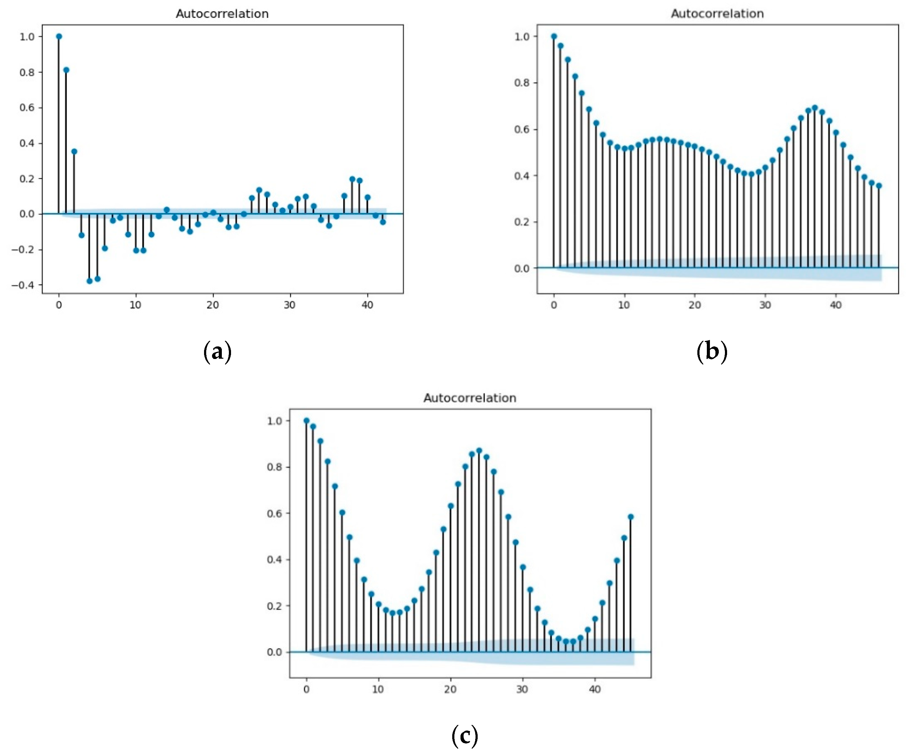
Figure 1. The autocorrelation function graph (a) The autocorrelation function graph of the MSO dataset; (b) the autocorrelation function graph of the humidity dataset; (c) the autocorrelation function graph of the power load dataset.
Mathematics 11 01503 g001
Figure 2. The structure of the ESN.
Mathematics 11 01503 g002
Figure 3. The structure of the DeepESN.
Mathematics 11 01503 g003
Figure 4. MSO dataset.
Mathematics 11 01503 g004
Figure 5. Humidity dataset.
Mathematics 11 01503 g005
Figure 6. Power load dataset.
Mathematics 11 01503 g006
Figure 7. The prediction results of different models for the MSO dataset.
Mathematics 11 01503 g007
Figure 8. Histogram of prediction errors of different models for the MSO dataset.
Mathematics 11 01503 g008
Figure 9. The prediction results of different models for the humidity dataset.
Mathematics 11 01503 g009
Figure 10. Histogram of prediction errors of different models for the Humidity dataset.
Mathematics 11 01503 g010
Figure 11. The prediction results of different models for the power load dataset.
Mathematics 11 01503 g011
Figure 12. Histogram of prediction errors of different models for the power load dataset.
Mathematics 11 01503 g012
Figure 13. Evaluation indicators of different optimization methods for the MSO dataset. (a) values of RMSE and MSE, (b) values of CC and R2, (c) running time.
Mathematics 11 01503 g013
Figure 14. Evaluation indicators of different optimization methods for the humidity dataset. (a) values of RMSE and MSE, (b) values of CC and R2, (c) running time.
Mathematics 11 01503 g014
Figure 15. Evaluation indicators of different optimization methods for the power load dataset. (a) values of RMSE and MSE, (b) values of CC and R2, (c) running time.
Mathematics 11 01503 g015
Table 1. The sample entropy of each dataset.
DatasetsData Interval 1
(0–500)
Data Interval 2
(500–1000)
Data Interval 3
(1000–1500)
Data Interval 4
(1500–2000)
MSO1.58741.53611.51411.6081
Humidity0.50500.72460.87050.8114
Power load0.63510.86710.90630.8376
Table 2. Statistical indicators for the three datasets.
DatasetsMinimumMaximumMeanStandard DeviationVariance
MSO−7.44417.3918−0.02612.00094.0034
Humidity61005326.267689.957
Power load719622,75914,784.7162388.07595,702,906
Table 3. The parameter ranges of the three datasets.
HyperparameterTypeMSO Data
Parameter Range
Humidity Data
Parameter Range
Power Load Data
Parameter Range
layersinteger1–301–401–30
Number of neuronsinteger100–4000100–4000100–6000
Leaking rateuniform0.1–1.00.1–1.00.1–1.0
Spectral radius rateuniform0.1–1.00.1–1.00.1–1.0
Input scalinguniform0.1–1.00.1–1.00.1–1.0
Table 4. Parameter setting for comparison models.
ModelLayersNumber of NeuronsReservoir SizeSpectral Radius RateLeaking Rate
BP324NANANA
LSTM132NANANA
GRU132NANANA
ESNNANA6000.90.2
Table 5. Evaluation indicators of the MSO dataset.
ModelRMSEMAECCR2
BP1.76071.39530.50450.2221
LSTM1.22520.92740.79820.6234
GRU1.42901.05350.70530.4876
ESN0.10240.08130.99870.9974
DeepESN0.07190.05730.99940.9987
Table 6. Evaluation indicators of the humidity dataset.
ModelRMSEMAECCR2
BP21.500315.62530.61380.2787
LSTM20.740515.21970.62490.3289
GRU19.004814.07150.68970.4365
ESN22.114617.31040.60690.2369
DeepESN18.670714.70070.67860.4561
Table 7. Evaluation indicators of the power load dataset.
ModelRMSEMAECCR2
BP801.637626.6600.89220.7926
LSTM840.739623.6280.89260.7719
GRU791.691583.0790.91150.7977
ESN823.565586.3550.89450.7811
DeepESN764.5281584.2960.90110.8114
Table 8. Prediction results of different optimization methods.
DatasetsOptimization MethodRMSEMAECCR2Time (s)
MSOBOA0.07190.05730.99940.9987323.4
MSOGrid search0.06890.05440.99960.99893587.2
MSOGWO0.12040.09710.98810.9855672.9
HumidityBOA18.670714.70070.67860.4561563.2
HumidityGrid search18.581914.68930.66290.43446023.3
HumidityGWO20.690717.35440.58030.3321964.1
Power loadBOA764.5281584.2960.90110.8114985.4
Power loadGrid search749.8249573.3540.92590.83199987.8
Power loadGWO796.5818613.1410.89340.79521367.2
Table 9. Parameters on each dataset obtained through Bayesian optimization.
DatasetsOptimization MethodLayersNumber of NeuronsLeaking RateSpectral Radius RateInput Scaling
MSOBOA1225000.200.790.10
MSOGrid search517000.390.440.26
MSOGWO1839980.370.710.10
HumidityBOA531000.890.820.03
HumidityGrid search316000.700.370.41
HumidityGWO61670.120.100.11
Power LoadBOA959000.990.470.29
Power LoadGrid search834000.290.360.28
Power LoadGWO954710.110.100.21
Disclaimer/Publisher’s Note: The statements, opinions and data contained in all publications are solely those of the individual author(s) and contributor(s) and not of MDPI and/or the editor(s). MDPI and/or the editor(s) disclaim responsibility for any injury to people or property resulting from any ideas, methods, instructions or products referred to in the content.