Exact Permutation and Bootstrap Distribution of Generalized Pairwise Comparisons Statistics

Abstract

To analyze multivariate outcomes in clinical trials, several authors have suggested generalizations of the univariate Mann–Whitney test. As the Mann–Whitney statistic compares the subjects’ outcome pairwise, the multivariate generalizations are known as generalized pairwise comparisons (GPC) statistics. For GPC statistics such as the net treatment benefit, the win ratio, and the win odds, asymptotic based or re-sampling tests have been suggested in the literature. However, asymptotic methods require a sufficiently high sample size to be accurate, and re-sampling methods come with a high computational burden. We use graph theory notation to obtain closed-form formulas for the expectation and the variance of the permutation and bootstrap sampling distribution of the GPC statistics, which can be utilized to develop fast and accurate inferential tests for each of the GPC statistics. A simple example and a simulation study demonstrate the accuracy of the exact permutation and bootstrap methods, even in very small samples. As the time complexity is $O\left(N^2\right)$, where N is the total number of patients, the exact methods are fast. In situations where asymptotic methods have been used to obtain these variance matrices, the new methods will be more accurate and equally fast. In situations where bootstrap has been used, the new methods will be both more accurate and much faster.

1. Introduction

In randomized clinical trials, often multiple outcome measures are selected to assess the effect of a treatment on two groups of subjects. In clinical areas, such as cardiology, oncology, psychology, and infectious disease, the combination of several clinical meaningful outcome measures is very common [1,2,3,4]. The standard method of analysis for multivariate survival outcomes is a time-to-first event analysis, which uses only the first event per subject [5]. However, this approach has been criticized, since it ignores subsequent events and the clinical relevance of the events. To remediate the shortcomings of the time-to-first event analysis, a new class of non-parametric methods has been proposed that allows for the analysis of multiple events per subject and allows for prioritizing the events by clinical relevance [6,7,8]. These methods are a generalization to multivariate prioritized outcomes of the classical univariate Mann–Whitney [9] and Gehan–Wilcoxon test [10,11]. Similar to the univariate outcome statistic, the generalized statistics compare the outcome per pair of subjects and hence are named generalized pairwise comparisons (GPC) statistics [7], while others use the term win statistics [12].

GPC is based on a prioritization of a number of k outcome measures, usually according to a decreasing level of clinical relevance. For each outcome measure, every subject is compared to every other subject in a pairwise manner. Per pair and per outcome, a score, $u_{ijk}$, is assigned, which is chosen to reflect whether subject i or subject j has the more favorable outcome k. The concept of more favorable can involve censoring, missing data, and can include a threshold of clinical relevance [7,13]. The score $u_{ijk}$ that is most often used is the score proposed by Gehan [10] for censored observations:

$$u_{ijk}=\left\{\begin{array}{cc}\hfill 1,& \mathrm{if}\mathrm{subject}i\mathrm{has}\mathrm{a}\mathrm{more}\mathrm{favorable}\mathrm{outcome}k\mathrm{than}\mathrm{subject}j\hfill \\ \hfill 0,& \mathrm{if}\mathrm{the}\mathrm{subjects}\mathrm{cannot}\mathrm{be}\mathrm{compared}\mathrm{on}\mathrm{outcome}k\mathrm{or}\mathrm{are}\mathrm{tied}\hfill \\ \hfill -1,& \mathrm{if}\mathrm{subject}i\mathrm{has}\mathrm{a}\mathrm{less}\mathrm{favorable}\mathrm{outcome}k\mathrm{than}\mathrm{subject}j\hfill \end{array}\right.$$

The scores can be computed separately for each outcome measure k, and the score $u_{ij}$ for a pair in the prioritized GPC is the first non-zero score $u_{ijk}$, where the first is defined by the prespecified priority list of outcomes. It is quite possible that for many pairs of subjects, the overall comparison will remain 0. It is also possible to have non-transitive comparisons, such as three patients where $u_{ij}=1$, $u_{jk}=1$, and $u_{ki}=1$ [13]. Alternatively, if prioritization of the outcome measures is not feasible or appropriate, a non-prioritized GPC sums the scores $u_{ijk}$ over all outcome measures [13,14]. Additionally, the scores of the pairs that are uninformative due to censored observations, and thus cannot be compared, can be corrected by estimating the chance of a favorable outcome using Kaplan–Meier estimates [15,16,17,18]. The Kaplan–Meier corrected score matrix will consist of scores $|u_{ij}|<1$. The score matrix resulting from the pairwise comparisons is a skew-symmetric $N\times N$ matrix, with entries in the set $\{-1,0,+1\}$ for the prioritized GPC without the censoring corrections and entries in $\mathbb{R}$ otherwise. Although scores in a non-prioritized GPC can be $>1$ per pair, most GPC statistics will adjust the scoring by dividing by k outcomes. Because of the summing, this adjustment can be performed at the level of the scores or after summing all scores. In the former, scores will be $|u_{ij}|<1$, while in the latter, scores will be $|u_{ij}|>1$.

Inferential tests and confidence intervals for GPC are then constructed from the scoring matrix, utilizing statistics such as the Finkelstein–Schoenfeld statistic [6], the net treatment benefit [7], the win ratio [8] and win odds [19]. Suppose there are N subjects in a two-arm trial, with m subjects in the experimental group from a distribution $F_1$ and n subjects in the control group from a distribution $F_2$. Moreover, let the indicator $D_i=1$ for subjects in the experimental group, and $D_i=0$ for patients in the control group. The Finkelstein–Schoenfeld statistic [6] is then the sum of the scores for the experimental group. If $U_i={\sum }_j{u}_{ij}$, the Finkelstein–Schoenfeld statistic is:

$$FS=\sum _{i=1}^N{D}_i{U}_i,$$

(1)

which can be interpreted as the difference between the favorable outcomes in the experimental arm, $W_T={\sum }_{i=1}^N{D}_i{U}_i$ with $u_{ij}>0$, and the favorable outcomes in the control arm, $W_C={\sum }_{i=1}^N{D}_i{U}_i$ with $u_{ij}<0$. If the score entries are restricted to $\{-1,0,+1\}$, $W_T$ and $W_C$ merely count the number of wins per treatment arm, and $FS=W_T-W_C$.

It is easy to show (Appendix A) that $\mathbb{E}\left(FS\right)=0$. The variance suggested by Finkelstein and Schoenfeld [6] is based on a permutation test

$$\mathrm{Var}\left(FS\right)={\displaystyle \frac{mn}{N(N-1)}}\sum _{i=1}^N{U}_i^2,$$

(2)

following [10,11,20]. Although Finkelstein and Schoenfeld presented the formula for $\mathrm{Var}\left(FS\right)$, they did not give expectations and variances for $W_T$ and $W_C$ separately. For many of the GPC models considered below, those separate variances are needed.

The permutation test assumes exchangeability between observations and tests the null hypothesis: $H_0:F_1=F_2$. Gehan [10], Gilbert [11] and Mantel [20] derived a closed-form expression of the mean and variance of the exact null distribution, which means that no re-sampling permutation is actually required. Consequently, the asymptotic null distribution of the test statistic $FS/\sqrt{\mathrm{Var}\left(FS\right)}$ is shown to be standard normal [10,11], and the p-values computed from this null distribution are valid, even for very small sample sizes of only 10 observations [10]. Alternatively, inference can be based on the proportion of re-sampling permutation samples with a test statistic greater than or equal to the observed statistic. Even though the permutation test is formulated under the $H_0$ null hypothesis, the test statistic is only consistent under alternatives of the form $FS\ne 0$ [10,11]. The permutation test is thus not consistent against all alternatives of the form $F_1\ne F_2$ [21,22].

Other GPC statistics include the net treatment benefit (NTB) [7], which is a U-statistic [23] transformation of the Finkelstein–Schoenfeld statistic, by dividing it by the total number of pairs possible between the two treatment arms, $(W_T-W_C)/\left(nm\right)$. It has been shown that the NTB and its transformations are unbiased and efficient estimators for univariate and uncensored observations [24]. The win ratio (WR) is defined as the ratio of the number of times a subject has a favorable outcome in the treatment arm and in the control arm, $W_T/W_C$ [8]. Finally, the win odds adds half of the number of tied outcomes ($W_0$) to both the numerator and denominator, $(W_T+1/2W_0)/(W_C+1/2W_0)$ [25]. Since the win odds ($WO$) is a transformation of the net treatment benefit, $WO=(1+NTB)/(1-NTB)$, any test proposed for the net treatment benefit or Finkelstein–Schoenfeld statistic can also be applied to the win odds, and we will not focus further on the win odds.

For the inference of the GPC statistics, also re-sampling bootstrap [8], re-sampling re-randomization [7] or U-statistic asymptotic methods have been proposed [14,26,27]. The asymptotic properties are used in two different ways:

• Asymptotic formulas for the mean and variances of the numbers of wins, $W_T$ and $W_C$, which are both U-statistics and thus asymptotically normal distributed [23]. Our method avoids the errors in these asymptotic formulas, since we give exact formulas.
• Delta method derivations of results for the win ratio based on the computed approximate means and variances.

For larger trials, the asymptotic formulas may be satisfactory, but the re-sampling methods require a large number of replications to be accurate. In contrast, the permutation test (2) presented by Finkelstein and Schoenfeld [6] avoids the first step in the use of asymptotic properties and the associated error. This would be important in smaller clinical trials, such as in rare disease trials. Moreover, as the permutation test is an exact test in finite sampling, it is more accurate than the re-sampling methods and less time-consuming.

While the permutation test, as derived by Gehan [10], can be easily extended to the net treatment benefit and the win odds through their transformations, it is not obvious to extend it to the win ratio. Moreover, the permutation test determines the variability under the null hypotheses, making it unsuited for the determination of a confidence interval of the GPC statistics. Therefore, we re-derive the closed-form expression of the expectation and the variance of the permutation distribution using graph theory notation on the skew-symmetric score matrix, which allows extension of these results to a two-sample bootstrap distribution and to the win ratio. Additionally, we generalize the expression to allow scores in the $\mathbb{R}$ field, generalizing the application to non-prioritized GPC algorithms and censoring correcting scores. It will be shown that the algorithm complexity of our expressions is $O\left(N^2\right)$ in both time and space, and thus, the exact permutation and bootstrap method will be both faster and more accurate than re-sampling permutation and bootstrap tests.

This paper is organized as follows. In Section 2, the graphical model is presented that will be used the derive the expected values and variances of the GPC statistic under the permutation and bootstrap distribution. The exact permutation formulas for the mean and variance are derived in Section 3, while the exact bootstrap formulas follow in Section 4. The time complexity of the exact methods is evaluated in Section 5. Throughout the development of the theory, a small example is used to demonstrate the new methodologies. Additionally, a simulation shows the type I error and the 95% confidence interval coverage in Section 6, and the methodology is demonstrated in an example in Section 7. Both R® and SAS code for the exact permutation, and bootstrap tests are presented in the Supplementary Material as well as full detailed derivations and an extensive test of the algorithm.

2. Graphical Model

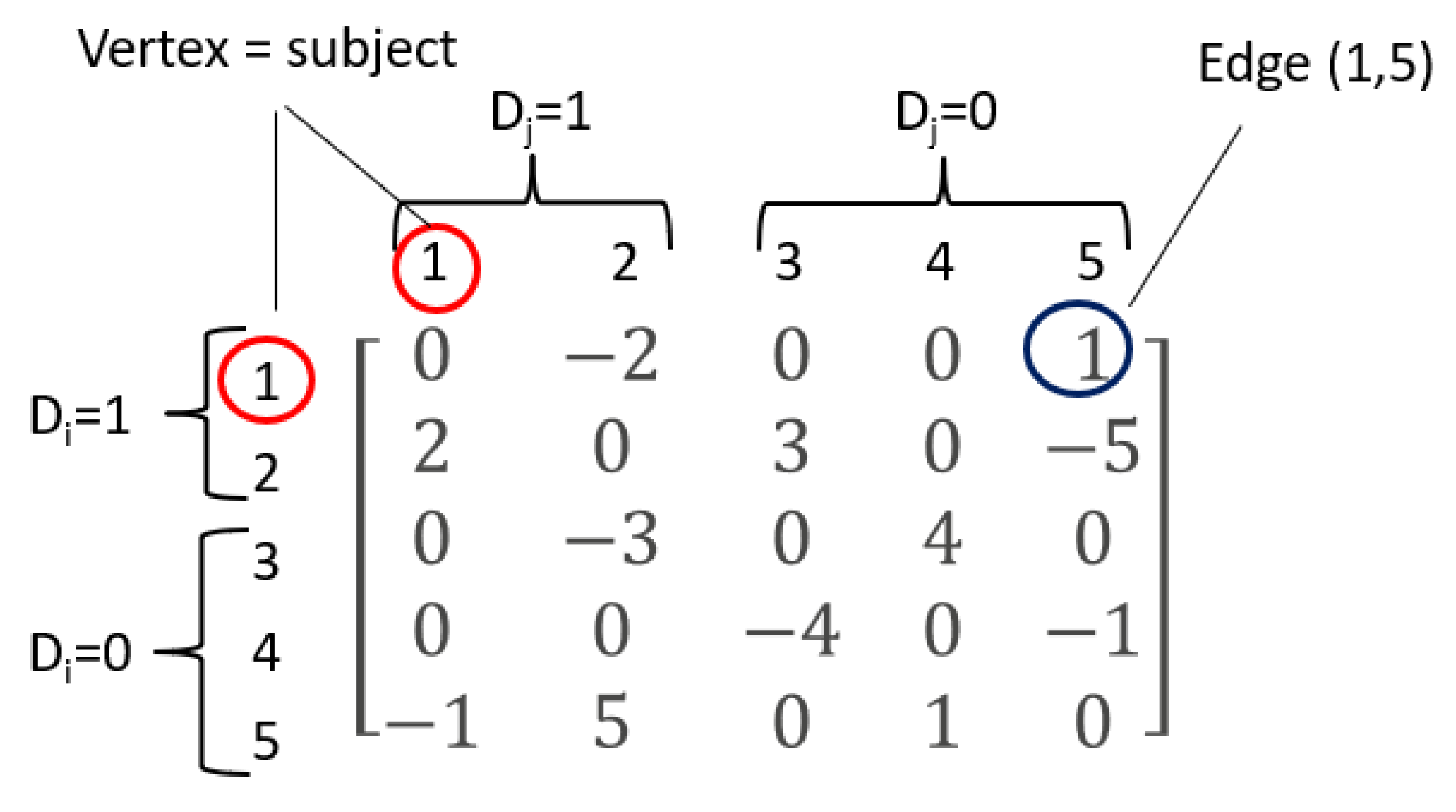
Any pairwise comparison analysis of an outcome measure in $N=n+m$ subjects, that allows for non-prioritized analyses and censoring corrected scores to denote the more favorable outcome, will result in a skew-symmetry $N\times N$ score matrix U with entries in the $\mathbb{R}$ field. This will be the case when evaluating both a single outcome measure, by use of the Mann–Whitney test, or the Gehan–Wilcoxon test, and when evaluating multiple outcomes, by a GPC analysis. In the remainder of this manuscript, we consider that the score matrix U has been produced by some further unspecified mechanism; the only restriction is the skewness and symmetry. A small example (Figure 1) illustrates such a U matrix.

Since all GPC statistics can be constructed from $W_T$ and $W_C$, it is our aim to compute the expectations and the variances of $W_T$ and $W_C$ as well as their covariance for both the permutation as the bootstrap distribution. These mean and (co)variances are computed over all possible permutations of the treatment arms or all possible bootstrap samples. For the net treatment benefit ($\Delta$),

$$\begin{array}{cc}\hfill \mathbb{E}(\Delta )& =\frac{\mathbb{E}\left(W_T\right)-\mathbb{E}\left(W_C\right)}{nm}\hfill \end{array}$$

(3)

$$\begin{array}{cc}\hfill \mathrm{Var}(\Delta )& =\frac{\mathrm{Var}\left(W_T\right)+\mathrm{Var}\left(W_C\right)-2\mathrm{Cov}\left(W_T{W}_C\right)}{{\left(nm\right)}^2}.\hfill \end{array}$$

(4)

For the win ratio $(\Psi )$, it is known that the logarithm of the win ratio is approximately normal distributed [24,26]. Its variance can then be approximated using the delta method:

$$\begin{array}{cc}\hfill \mathbb{E}(\Psi )& \approx \frac{\mathbb{E}\left(W_T\right)}{\mathbb{E}\left(W_C\right)}\hfill \end{array}$$

(5)

$$\begin{array}{cc}\hfill \mathrm{Var}(log\Psi )& \approx \frac{\mathrm{Var}\left(W_T\right)}{W_T^2}+\frac{\mathrm{Var}\left(W_C\right)}{W_C^2}-2\frac{\mathrm{Cov}\left(W_T{W}_C\right)}{W_T{W}_C}.\hfill \end{array}$$

(6)

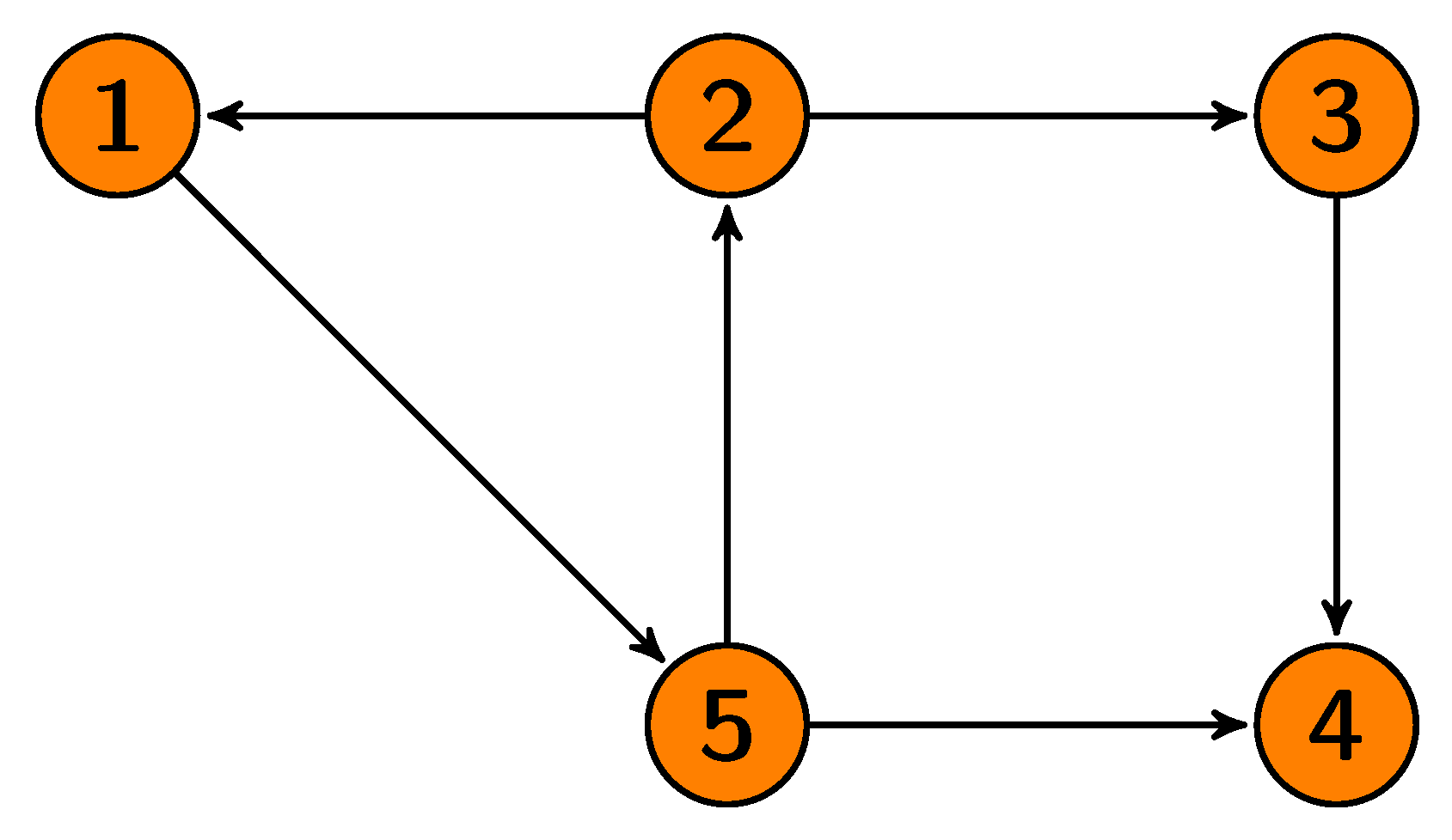
In order to derive the expectations, variances, and covariance for the $W_T$ and $W_C$, it will be convenient to think of the score matrix U as the adjacency matrix of a directed graph $\mathbb{G}$ [28] with N vertices, where a vertex represents a subject. A pair of subjects or vertices can be joined by an edge $e=(i,j)$. Since we are interested in the favorable outcomes, an edge $e=(i,j)$ is defined when $u_{ij}>0$. When $D_i=1$ and $D_j=0$, such an edge is called a treatment edge and when $D_i=0$ and $D_j=1$, it is called a control edge. The value $u_{ij}$ is called the weight of the edge, and it is denoted by $w_e$. Note that the score of the comparison of subject i with subject j is exactly the opposite of the score of the comparison of subject j with subject i. Hence, the edge $e=(i,j)$ is an ordered pair of distinct vertices, where the head of e is vertex j and the tail is vertex i. In a pictorial representation, the edge $e=(i,j)$ is represented by an arrow going from vertex i to vertex j (Figure 2). Let then E denote the total number of edges of $\mathbb{G}$. In our small example (Figure 1 and Figure 2), $E=6$.

Using the graph theory notation, the number of wins for the treatment, $W_T$, and control arm, $W_C$, can be redefined as follows. For a subject or vertex v, let $N_v$ denote the number of times that the vertex v appears in the sample. In a permutation sample, each subject can only appear once and $N_v=1$ for all samples. In a bootstrap sample, subjects can appear more than once and $N_v$ can be zero or higher. To count the number of wins for the treatment arm, the value $T_e$ is defined as the number of times that edge e is a treatment edge in the sample, and similarly, the value $C_e$ is the number of times that edge e is a control edge. If the treatment edge e has subjects $(v,w)$, the number of times this edge appears in the sample is then $T_e=N_v{N}_w$. For example, suppose that in a bootstrap sample of the five subjects in our small example (Figure 1), subjects 1 and 2 appear twice, subject 3 appears once, and subjects 4 and 5 do not appear at all; then, $N_1=N_2=2$, $N_3=1$, and $N_4=N_5=0$. Furthermore, the pair or treatment edge (2,1) will appear $T_{e(2,1)}=N_1\times N_2=4$ times, the treatment edge $T_{e(2,3)}=2$ times and all other treatments edges $T_e=0$ times. The vectors T and C are the $E\times 1$ column vectors composed of the various $T_e$ and $C_e$ and the vector W is the column vector of the weights $w_e$.

$W_T$ and $W_C$ are then redefined as:

$$\begin{array}{cc}\hfill W_T& ={\mathbf{W}}^t\mathbf{T}=\sum _e{w}_e{T}_e=[w_1,w_2,\dots ,w_E]\mathbf{T}\hfill \\ \hfill W_C& ={\mathbf{W}}^t\mathbf{C}=\sum _e{w}_e{C}_e=[w_1,w_2,\dots ,w_E]\mathbf{C}\hfill \end{array}$$

In our small example (Figure 1):

• Vector of edges = {(1,5),(2,1),(2,3),(3,4),(5,2),(5,4)};
• Vector ${\mathit{W}}^{\mathit{t}}$ = {1,2,3,4,5,1};
• Vector ${\mathit{T}}^{\mathit{t}}$ = {1,0,1,0,0,0} and $W_T=4$;
• Vector ${\mathit{C}}^{\mathit{t}}$ = {0,0,0,0,1,0} and $W_C=5$.

The development of the expectations and variances of $W_T$ and $W_C$, and their covariance for the permutation and the bootstrap distribution, then follow the same general pattern.

The expectation of $W_T$ is derived by:

$$\begin{array}{cc}\hfill \mathbb{E}\left(W_T\right)& =\mathbb{E}\left({\mathbf{W}}^t\mathbf{T}\right)\hfill \\ \hfill & =[w_1,w_2,\dots ,w_E]\mathbb{E}\left(\mathbf{T}\right)\hfill \\ \hfill & =\sum _e{w}_e\mathbb{E}\left(T_e\right).\hfill \end{array}$$

and similarly, $\mathbb{E}\left(W_C\right)={\sum }_e{w}_e\mathbb{E}\left(C_e\right)$.

The variance is derived by

$$\begin{array}{cc}\hfill \mathrm{Var}\left([W_T,W_C]\right)& =\mathrm{Var}\left(\left[\begin{array}{c}{\mathbf{W}}^t,{\mathbf{W}}^t\end{array}\right]\left[\begin{array}{c}\mathbf{T}\\ \mathbf{C}\end{array}\right]\right)\hfill \\ \hfill & =\left[\begin{array}{c}{\mathbf{W}}^t,{\mathbf{W}}^t\end{array}\right]\mathrm{Var}\left(\left[\begin{array}{c}\mathbf{T}\\ \mathbf{C}\end{array}\right]\right)\left[\begin{array}{c}\mathbf{W}\\ \mathbf{W}\end{array}\right]\hfill \\ \hfill & =\left[\begin{array}{c}{\mathbf{W}}^t,{\mathbf{W}}^t\end{array}\right]\left(\mathbb{E}\left(\left[\begin{array}{c}\mathbf{T}\\ \mathbf{C}\end{array}\right]{\left[\begin{array}{c}\mathbf{T}\\ \mathbf{C}\end{array}\right]}^t\right)-\left(\mathbb{E}\left[\begin{array}{c}\mathbf{T}\\ \mathbf{C}\end{array}\right]\right)\left(\mathbb{E}{\left[\begin{array}{c}\mathbf{T}\\ \mathbf{C}\end{array}\right]}^t\right)\right)\left[\begin{array}{c}\mathbf{W}\\ \mathbf{W}\end{array}\right]\hfill \\ \hfill & =\left[\begin{array}{c}{\mathbf{W}}^t,{\mathbf{W}}^t\end{array}\right]\left(\mathbb{E}\left(\left[\begin{array}{cc}\mathbf{T}{\mathbf{T}}^t& \mathbf{T}{\mathbf{C}}^t\\ \mathbf{C}{\mathbf{T}}^t& \mathbf{C}{\mathbf{C}}^t\end{array}\right]\right)-\left[\begin{array}{cc}\mathbb{E}\left(\mathbf{T}\right)\mathbb{E}\left({\mathbf{T}}^t\right)& \mathbb{E}\left(\mathbf{T}\right)\mathbb{E}\left({\mathbf{C}}^t\right)\\ \mathbb{E}\left(\mathbf{C}\right)\mathbb{E}\left({\mathbf{T}}^t\right)& \mathbb{E}\left(\mathbf{C}\right)\mathbb{E}\left({\mathbf{C}}^t\right)\end{array}\right]\right)\left[\begin{array}{c}\mathbf{W}\\ \mathbf{W}\end{array}\right]\hfill \end{array}$$

(7)

$$\begin{array}{cc}\hfill & =\left[\begin{array}{cc}{V}_{TT}& V_{TC}\\ V_{CT}& V_{CC}\end{array}\right]\hfill \end{array}$$

(8)

The variance of the GPC statistics thus requires two counting steps. In the first step, the expected values $\mathbb{E}\left(T_e\right)$, $\mathbb{E}\left(C_e\right)$ and the expected value of an ordered pair of edges $(e,f)$, not necessarily distinct, $\mathbb{E}\left(T_e{T}_f\right)$, $\mathbb{E}\left(T_e{C}_f\right)$, $\mathbb{E}\left(C_e{T}_f\right)$, and $\mathbb{E}\left(C_e{C}_f\right)$ are computed using elementary calculations involving binomial coefficients. These calculations differ between edge pairs, depending on the trial arm assignments and the geometric relationship of the edges. Note that because the variance matrix is symmetric, we do not explicitly need the individual terms $\mathbb{E}\left(C_e{T}_f\right)$. In the second step, the number of times that each of these geometric configurations of edges is present in the data set is counted.

3. The Permutation Distribution

In this section, it is shown that our derivation of the graph theory concepts lead to the exact same permutation test as proposed by Gehan [10], Gilbert [11], Mantel [20] and Finkelstein and Schoenfeld [6]. It allows, however, to develop a permutation test for the win ratio, and it can be extended to a bootstrap test.

In a permutation test, subjects are randomly re-sampled to the treatment groups without replacement. If all $\left(\genfrac{}{}{0pt}{}{m+n}{m}\right)$ possible permutations of m treatment assignments and n control assignments are considered, the $W_T$ and $W_C$ in each of these permutation samples will lead to their permutation distribution. The expectations, variances, and covariance of this permutation distribution of $W_T$ and $W_C$ can be calculated explicitly. An edge will thus always join the same subjects, but whether or not this edge contributes to the treatment wins or control wins depends on the treatment assignment in the permutation sample.

The expectations of $W_T$ and $W_C$ are the same in the permutation distribution (Supplementary Material S1 Section S4.1):

$${\mathbb{E}}_P\left(W_T\right)={\mathbb{E}}_P\left(W_C\right)={\displaystyle \frac{mn}{N(N-1)}}\sum _e{w}_e.$$

These provide the second half of the Equation (7). For our small example (Figure 1), the expectations of $W_T$ and $W_C$ equal ${\displaystyle \frac{6}{5\times 4}}(1+2+3+4+5+1)=4.8$.

The variance for the treatment wins, $W_T$, is then (Supplementary Material S1 Section S4.3)

$$\begin{array}{cc}\hfill {\mathrm{Var}}_P\left(W_T\right)=& {\displaystyle \frac{mn}{N(N-1)}}\sum _v{I}_v^s+{\displaystyle \frac{mn(m-1)}{N(N-1)(N-2)}}\sum _v(I_v^2-I_v^s)+{\displaystyle \frac{mn(n-1)}{N(N-1)(N-2)}}\sum _v(O_v^2-O_v^s)\hfill \\ \hfill & +{\displaystyle \frac{mn(m-1)(n-1)}{N(N-1)(N-2)(N-3)}}\left\{{(\sum _v{I}_v)}^2-\sum _v\left[I_v^s+(I_v^2-I_v^s)+(O_v^2-O_v^s)+2I_v{O}_v\right]\right\}\hfill \\ \hfill & -{\left[{\displaystyle \frac{mn}{N(N-1)}}\sum _v{I}_v\right]}^2,\hfill \end{array}$$

with

$$\begin{array}{cc}\hfill I_v& =\sum _i{w}_e\mathrm{the}\mathrm{column}\mathrm{sums}\mathrm{of}{w}_e\mathrm{for}\mathrm{vertex}v.\hfill \\ \hfill I_v^s& =\sum _i{w}_e^2\mathrm{the}\mathrm{column}\mathrm{sums}\mathrm{of}{w}_e^2\mathrm{for}\mathrm{vertex}v.\hfill \\ \hfill O_v& =\sum _j{w}_e\mathrm{the}\mathrm{row}\mathrm{sums}\mathrm{of}{w}_e\mathrm{for}\mathrm{vertex}v.\hfill \\ \hfill O_v^s& =\sum _j{w}_e^2\mathrm{the}\mathrm{row}\mathrm{sums}\mathrm{of}{w}_e^2\mathrm{for}\mathrm{vertex}v.\hfill \end{array}$$

Note that ${\sum }_v{I}_v={\sum }_v{O}_v={\sum }_e{w}_e$ and that, due to the symmetry of the U-matrix, the column sums of $w_e$ (or entries with $u_{ij}>0)$ are equal to the row sums of $u_{ij}<0$.

The variance for $W_C$ is similar, but with the roles of $I_v$ and $O_v$ reversed. The covariance of $W_T$ and $W_C$ equals (Supplementary Material S1 Section S4.3):

$$\begin{array}{cc}\hfill {\mathrm{Cov}}_P\left(W_T{W}_C\right)=& {\displaystyle \frac{mn}{N(N-1)}}\sum _v{I}_v{O}_v+{\displaystyle \frac{mn(m-1)(n-1)}{N(N-1)(N-2)(N-3)}}\left\{{(\sum _v{I}_v)}^2-\sum _v\left[I_v^s+(I_v^2-I_v^s)\right.\right.\hfill \\ \hfill & \left.\left.+(O_v^2-O_v^s)+2I_v{O}_v\right]\right\}-{\left[{\displaystyle \frac{mn}{N(N-1)}}\sum _v{I}_v\right]}^2\hfill \end{array}$$

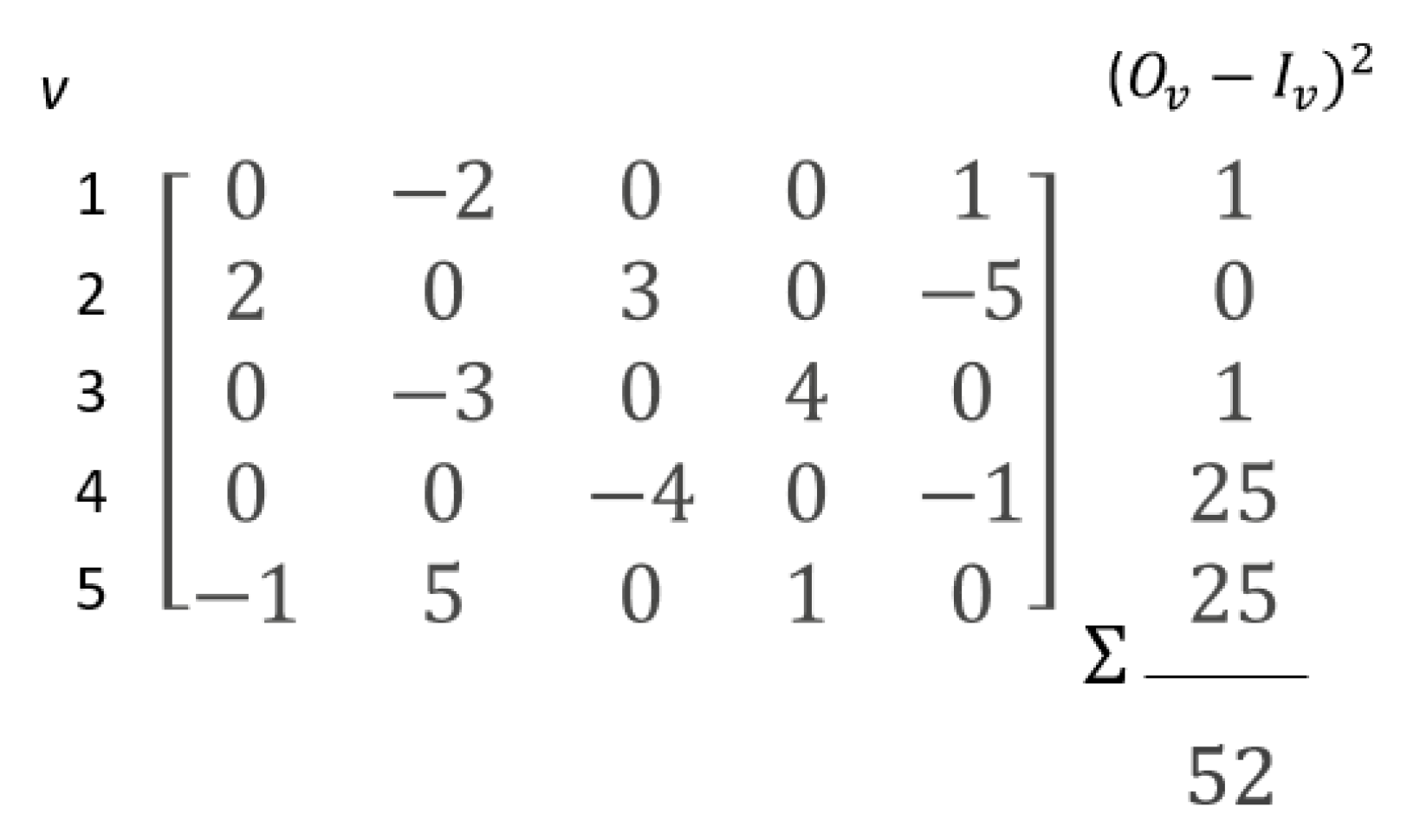
Finally, the variance of the Finkelstein–Schoenfeld statistic, the net treatment benefit and win ratio statistic can be calculated from (3)–(6). For the Finkelstein–Schoenfeld statistic (and the net treatment benefit), the exact permutation variance simplifies to simple row sums of $u_{ij}$ (Figure 3):

$$\begin{array}{cc}\hfill {\mathrm{Var}}_P(W_T-W_C)& ={\mathrm{Var}}_P\left(W_T\right)+{\mathrm{Var}}_P\left(W_C\right)-2{\mathrm{Cov}}_P\left(W_T{W}_C\right)\hfill \\ \hfill & =\frac{mn}{N(N-1)}(\sum _v{O}_v^2-2\sum _v{I}_v{O}_v+\sum _v{I}_v^2)\hfill \\ \hfill & =\frac{mn}{N(N-1)}\sum _v{(O_v-I_v)}^2\hfill \end{array}$$

It is easy to see that this is equal to (2), as proposed by Gehan [10], Gilbert [11], Mantel [20] and Finkelstein and Schoenfeld [6].

For our small example (Figure 1), it is possible to take every permutation sample, calculate the win difference for each sample and determine the variance of the win differences. If we do this, the variance coincides with what is calculated using the exact permutation formulas (see Supplementary Material S2, Section S1.1):

$${\mathrm{Var}}_P(W_T-W_C)=\frac{6}{5\times 4}\times 52=15.6.$$

Other examples can be found in Supplementary Material S2, Section S1.2.

4. The Bootstrap Distribution

Using a similar approach, we can now also develop a closed-form formula for the bootstrap distribution for both the net treatment benefit and the win ratio rather than the originally proposed re-sampling bootstrap test [8] for testing the hypothesis $H_0:\Delta =0$ or $H_0:\Psi =1$ or for the confidence interval construction.

In a bootstrap, subjects are randomly re-sampled with replacement within their treatment group. If all possible bootstrap samples, $m^m{n}^n$ in total, are considered, the number of treatment wins, $W_T$ and control wins, $W_C$, in each of these samples will lead to their bootstrap distribution. The expectations, variances, and covariance of this bootstrap distribution of $W_T$ and $W_C$ can also be calculated explicitly, following a similar reasoning as in the permutation. This method will be more accurate than actually re-sampling via bootstrap, since the randomization error is eliminated.

Since the bootstrap uses the same observed information as the permutation, the graph $\mathbb{G}$ described in Section 2 remains useful. The edges and vertices remain the same as previously. However, since an edge e can now be repeated in a sample, be present once, or not be present at all, the number of times an edge contributes to a win in T or C can now be between 0 and n, respectively, m. Additionally, since subjects or vertices remain in their treatment arm over the bootstrap samples, edges joining vertices within the same treatment arm ($D_i=D_j$) will never be a win in any bootstrap sample, and they will also not contribute to the variance. In other words, the variance of wins in a bootstrap sample does not depend on the within-arm comparisons. This is in contrast to the permutation variance, where within-arm comparisons contribute to the final variance.

There are thus ${(W_T+W_C)}^2$ ordered pairs of edges corresponding to wins and contributing to the variance. Let the indicator $D_v=1$ when $D_i=1$ and $D_j=0$, and $D_v=0$ when $D_i=0$ and $D_j=1$. An edge corresponding to a treatment win ($u_{ij}>0$ for $D_v=1$ and $u_{ij}<0$ for $D_v=0$) or a control win ($u_{ij}<0$ for $D_v=1$ and $u_{ij}>0$ for $D_v=0$) in the observed data will be called a treatment edge or a control edge.

One could also consider bootstrap sampling from the entire population to test the same null hypothesis of the permutation test, $H_0:F_1=F_2$. The formulas of the one-sample bootstrap are similar in spirit to those given here, and they are detailed in the Supplementary Material S1, Section S6.

Using elementary sums of multinomial coefficients, the expectations of $W_T$ and $W_C$ are shown to be ${\mathbb{E}}_B\left(W_T\right)={\sum }_e{w}_e{T}_e=W_T$ and similarly, ${\mathbb{E}}_B\left(W_C\right)={\sum }_e{w}_e{C}_e=W_C$ (Supplementary Material S1, Section S5.1). Consequently, the expectation of the win difference ${\mathbb{E}}_B(W_T-W_C)=W_T-W_C$ and the approximation of the expectation for the win ratio ${\mathbb{E}}_B\left(W_T\right)/{\mathbb{E}}_B\left(W_C\right)=W_T/W_C$.

The variance for the treatment wins, $W_T$, is then (Supplementary Material S1 Section S5.3)

$${\mathrm{Var}}_B\left(W_T\right)=\sum _{D_v=1}\#{\mathbb{T}}_v^s+\frac{n-1}{n}\sum _{D_v=1}\#{\mathbb{T}}_v^2+\frac{m-1}{m}\sum _{D_v=0}\#{\mathbb{T}}_v^2-\frac{m+n-1}{nm}{W}_T^2$$

(9)

with

$$\begin{array}{cc}\hfill \#{\mathbb{T}}_v& =\sum w_e\mathrm{the}\mathrm{row}\left(D_{v=1}\right)\mathrm{and}\mathrm{column}\left(D_{v=0}\right)\mathrm{sums}\mathrm{of}{w}_e>0\mathrm{for}\mathrm{vertex}v.\hfill \\ \hfill \#{\mathbb{T}}_v^s& =\sum w_e^2\mathrm{the}\mathrm{row}\left(D_{v=1}\right)\mathrm{and}\mathrm{column}\left(D_{v=0}\right)\mathrm{sums}\mathrm{of}{w}_e^2\mathrm{for}{w}_e>0\mathrm{vertex}v.\hfill \end{array}$$

The variance of $W_C$ is obtained similarly by replacing all treatment with control parameters and defining $\#{\mathbb{C}}_v$ as the row ($D_{v=1}$) and column ($D_{v=0}$) sums of $w_e<0$ for vertex v and $\#{\mathbb{C}}_v^s$ as the row ($D_{v=1}$) and column ($D_{v=0}$) sums of $w_e^2$ for $w_e<0$ vertex v. The covariance equals (Supplementary Material S1 Section S5.3):

$${\mathrm{Cov}}_B\left(W_T{W}_C\right)=\frac{n-1}{n}\sum _{D_v=1}\#{\mathbb{T}}_v\#{\mathbb{C}}_v+\frac{m-1}{m}\sum _{D_v=0}\#{\mathbb{T}}_v\#{\mathbb{C}}_v-\frac{m+n-1}{nm}{W}_T{W}_C$$

(10)

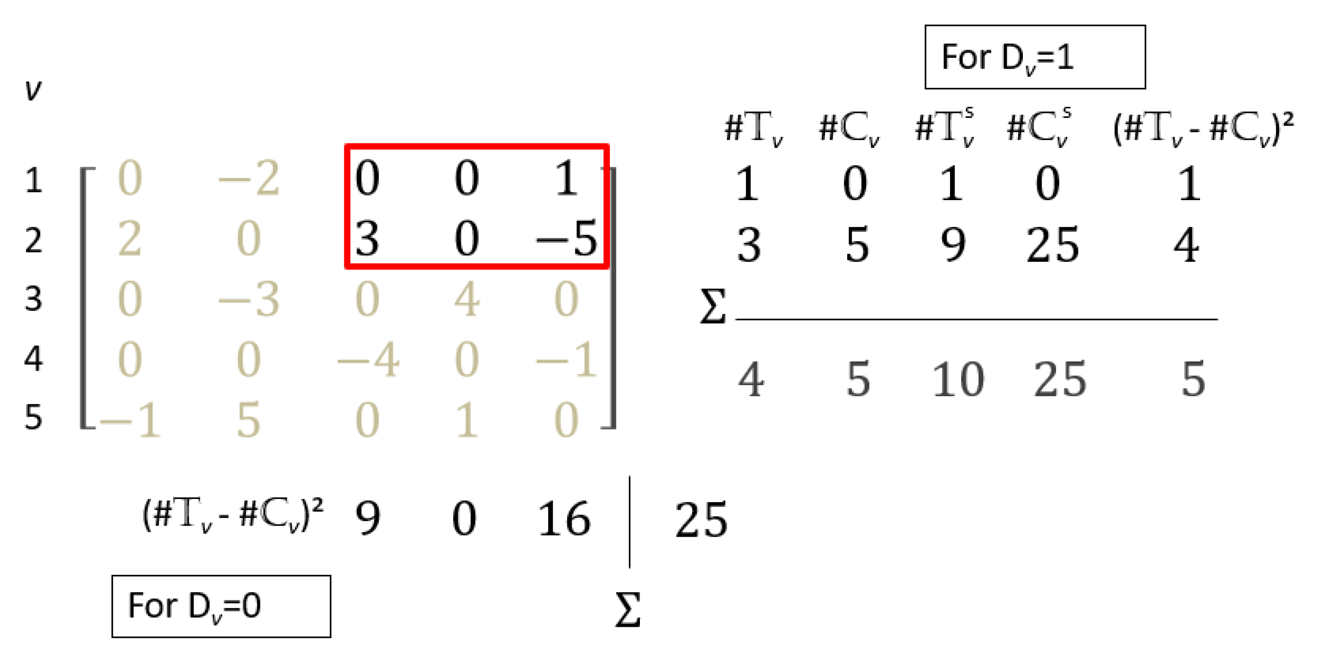
Finally, the variance of the Finkelstein–Schoenfeld statistic, the net treatment benefit and win ratio statistic can be calculated from (3)–(6). For the Finkelstein–Schoenfeld statistic and the net treatment benefit, the exact bootstrap variance simplifies to row and column sums of $\#\mathbb{T}$ and $\#\mathbb{C}$ counts (Figure 4).

For our small example (Figure 1), it is possible to take every bootstrap sample, calculate the win difference for each sample and determine the variance of the win differences. If we do this, the variance coincides with what is calculated using the exact bootstrap formulas (see Supplementary Material S2, Section S2.1):

$$\begin{array}{cc}\hfill {\mathrm{Var}}_B(W_T-W_C)& ={\mathrm{Var}}_B\left(W_T\right)+{\mathrm{Var}}_B\left(W_C\right)-2{\mathrm{Cov}}_B\left(W_T{W}_C\right)\hfill \\ \hfill & =\frac{n-1}{n}\left[\sum _{D_v=1}{(\#{\mathbb{T}}_v-\#{\mathbb{C}}_v)}^2\right]+\frac{m-1}{m}\left[\sum _{D_v=0}{(\#{\mathbb{T}}_v-\#{\mathbb{C}}_v)}^2\right]\hfill \\ \hfill & +\sum _{D_v=1}\#{\mathbb{T}}_v^s+\sum _{D_v=1}\#{\mathbb{C}}_v^s-\frac{m+n-1}{nm}{(W_T-W_C)}^2\hfill \\ \hfill & =\frac{2}{3}\left(5\right)+\frac{1}{2}\left(25\right)+10+25-\frac{4}{6}{(4-5)}^2=50.17\hfill \end{array}$$

Other examples can be found in Supplementary Material S2, Section S2.2.

5. Complexity

In any GPC analysis, a bounded number of computations for each pair of patients is performed to obtain the score matrix U, and the number of pairs is $O\left(N^2\right)$. The complexity of computing U is therefore $O\left(N^2\right)$. It is conceivable that one could reduce the complexity for special cases of GPC, however, our analysis works for arbitrary skew matrices, and in such cases, every pair of patients must be examined at least once.

For the variance of a GPC statistic, one could in principle consider all possible permutations or bootstrap samples, compute the numbers of treatment and control wins for each sample, and then compute the mean and variances. Such a computation would be exponential in N and hence completely unsatisfactory for a real example. We have performed such computations in some very small examples as a test of our algorithm (Supplementary Material S2).

For a specific vertex v, in order to compute the various vertex-dependent terms in the variance formulas, ($I_v$, $I_v^s$, $O_v$, $O_v^s$, $\#{\mathbb{T}}_v$, $\#{\mathbb{C}}_v$, $\#{\mathbb{T}}_v^s$, and $\#{\mathbb{C}}_v^s$), each other vertex must be examined once. Thus, the complexity of the computation at each vertex is $O\left(N\right)$, and computing at all vertices is thus $O\left(N^2\right)$. The total number of edges and the wins $W_T$ and $W_C$ are computed from these numbers in an additional $O\left(N\right)$ steps, and the final computations are $O\left(1\right)$. Accordingly, the time complexity of both the permutation and bootstrap algorithms is $O\left(N^2\right)$.

The exact computations will be faster than evaluating a large number of any permutation or bootstrap re-sampling, because evaluating only one sample is already $O\left(N^2\right)$.

6. Simulations

Similarly as for the Finkelstein-Schoenfeld test, inference for the permutation and bootstrap test is based on the standard normal assumption for the net treatment benefit and lognormal assumption for the win ratio of the asymptotic distribution of the permutation and bootstrap test statistic. While both the permutation and the bootstrap serve for hypothesis testing, albeit testing slightly different null hypotheses (see Introduction), only the bootstrap is additionally useful for confidence interval construction. As the permutation is estimating the variance under the null hypothesis, it is expected that the estimation bias of the variance under the alternative hypothesis will increase with increasing effect size. Since the bootstrap is estimating the variance under the alternative hypothesis, the bootstrap asymptotic distribution may be more likely to deviate from normality close to the boundary of potential values, which is 1 (or −1) for the NTB. Therefore, we will additionally evaluate an inverse hyperbolic tangent transformation of the test statistic, which limits the confidence interval within the boundaries of the NTB and under which the normality assumption may hold for smaller sample sizes [29].

By means of a simulation study, the appropriateness of the normality assumption is evaluated by means of the nominal type I error and the confidence interval coverage for small samples. The simulated samples contain 5, 10, 15, 20, 25, 30, 40, 50 or 75 observations from a normal distribution $N(0.3,0.1)$ for the experimental arm and an equal number of observations from a $N(\mu ,0.1)$ distribution with $\mu =0.3,0.264,0.205,0.119$ for the control arm. These correspond to a net treatment benefit of 0, 0.2, 0.5 and 0.8. Each simulation is repeated 10,000 times.

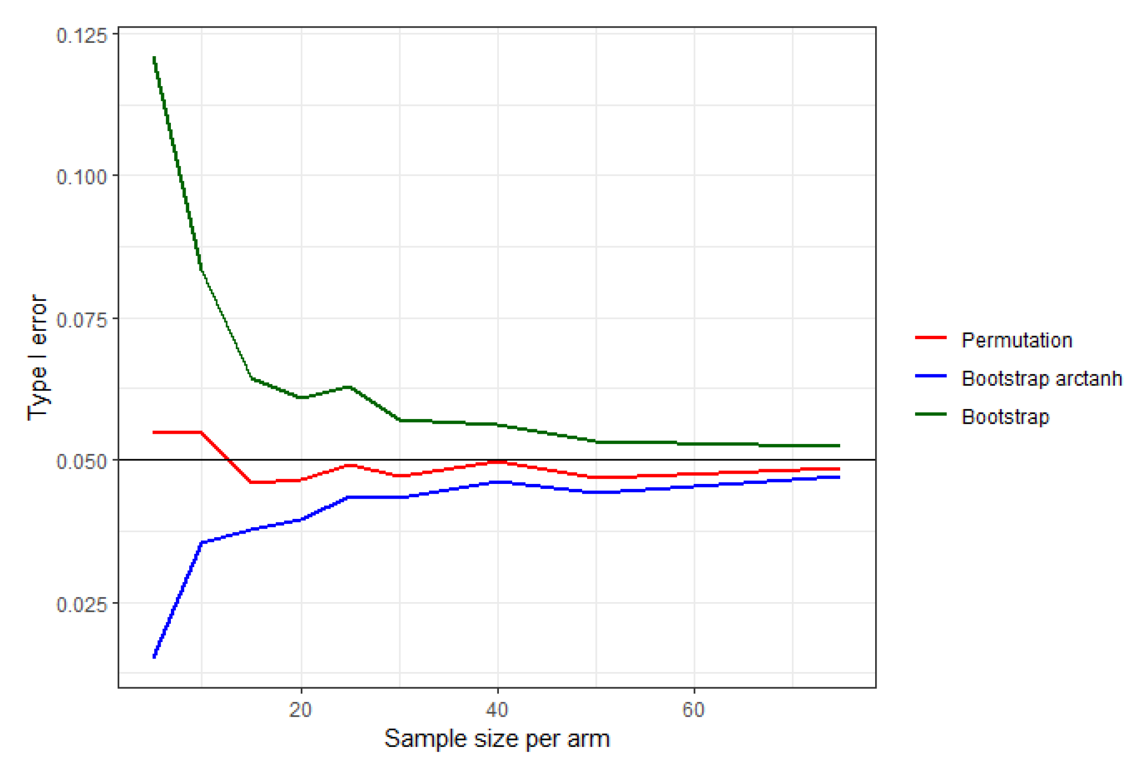
The permutation test controls the nominal alpha level well, even for very small sample sizes of five observations per treatment arm (Figure 5). The bootstrap test and its inverse hyperbolic tangent transformation on the other hand require at least 30–40 observations per treatment arm.

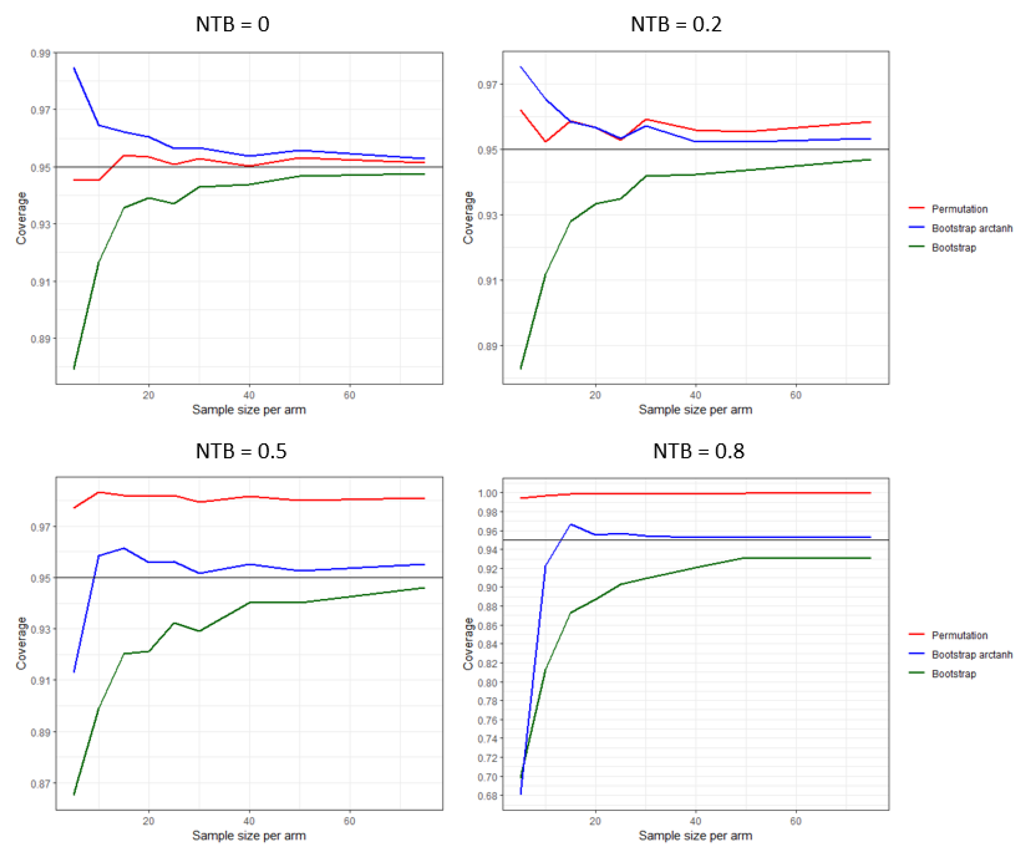
As anticipated, the confidence interval coverage based on the permutation distribution is good under the null hypothesis, but it increasingly deteriorates with increasing effect size (Figure 6). The coverage for the transformed bootstrap is for all effect sizes better in range than the untransformed bootstrap, and depending on the effect size requires 20–30 observations per treatment arm.

Further evaluation of the permutation and bootstrap Type I error control and confidence interval coverage, in comparison with other GPC methods for inference and with other type of data, is available in Verbeeck et al. [30].

7. Illustration

The rare, genetic skin disease epidermolysis bullosa simplex (EBS) is characterized by the formation of blisters under low mechanical stress [31]. An innovative immunomodulatory 1% diacerein cream was postulated to reduce the number of blisters compared to placebo and evaluated in a randomized, placebo-controlled, double-blind, two-period cross-over phase II/III trial in 16 pediatric patients [32]. After daily treatment during 4 weeks and monitoring for an additional 3 months, patients crossed over to the opposite treatment after a washout period. In each treatment period, both the number of blisters in a treated body surface area were counted and the quality of life (QoL) was assessed. The primary endpoint, the proportion of patients with more than 40% reduction in blisters at week 4 compared to baseline, however, leads to inconclusive results [32]. The primary analysis with the Barnard [33] test requires separate analyses per treatment period, which showed that during the first treatment period, there was a treatment effect in favor of the diacerein cream (p = 0.007) in contrast to the second treatment period (p = 0.32). Wally et al. [32] discuss reasons why the second period effect might be smaller.

Since the Barnard test is ignoring the cross-over design and the QoL, it only uses a fraction of the available information in the EBS trial. It is well known that the QoL of EBS patients is poor due to the hindrance of daily activities by the blisters [32]. While the reduction in the number of blisters is important, the healing but not yet disappearance of a blister may affect positively the QoL outcome, which is relevant for both the patient and clinician. The ability to add the QoL outcome with the blister outcome is clinically very relevant and very straightforward with GPC. We will re-analyze the EBS trial with a GPC both when prioritizing and not prioritizing the outcomes. Although GPC variants exist for matched designs [34], such as cross-over trials, under certain circumstances, which are applicable in the general GPC test, the matching can be ignored [35]. This means that we can consider the contribution of each subject to both treatment periods as a contribution of two independent subjects. Hence, the re-analysis will include all available information in a single analysis, which evades difficulties in interpreting conflicting results from separate analyses per treatment period.

The GPC permutation hypothesis test of the binary 40% reduction in blisters outcome and the continuous change in QoL outcome separately does not show evidence of a treatment effect of diacerin on the reduction in blisters ($p=0.0701$), while there is evidence for improvement in QoL ($p=0.0019$) (

Table 1. EBS trial data analysis of the composite blister and QoL outcomes with the prioritized and non-prioritized GPC. $W_T$ = number of wins for the diacerein arm, $W_C$ = number of wins for the placebo arm, $W_0$ = number of ties, NTB = net treatment benefit, CI = confidence interval.

	${\mathit{W}}_{\mathit{T}}$	${\mathit{W}}_{\mathit{C}}$	${\mathit{W}}_0$	NTB (95%CI)	p-Value Two-Sided
	Prioritized GPC
Blister	99 (44%)	24 (11%)		0.33
QoL	72 (32%)	14 (6%)		0.26
Total	171 (76%)	38 (17%)	16 (7%)	0.59 (0.19;0.82)	0.0051
	Non-Prioritized GPC
Blister	99 (44%)	24 (11%)	102 (45%)	0.33	0.0701
QoL	162 (72%)	22 (10%)	41 (18%)	0.62	0.0019
Total				0.48 (0.21;0.68)	0.0022

). In a prioritized GPC permutation test, where the blisters are evaluated first in the pairwise comparisons, there is evidence for a positive treatment effect of diacerin ($p=0.0051$) (Table 1). In addition, when evaluating all pairs for both outcomes in a non-prioritized GPC, the permutation test shows evidence for a positive treatment effect ($p=0.0022$) (Table 1). In addition, the confidence intervals around the net treatment benefit, obtained using the inverse hyperbolic tangent bootstrap, show that there is evidence for a treatment effect by diacerein, 59% (95% CI: 19–82%) with the prioritized GPC and 48% (95% CI:21–68%) for the non-prioritized GPC (Table 1).

8. Discussion

Efficient closed-form formulas to compute the expectation and the variance of the permutation and bootstrap distribution of GPC statistics are developed using graph theory notation. These methodologies are shown to give the exact means and variances and are not subject to sampling errors, which do result from any randomized permutation or bootstrap test. Additionally, it is shown that the time complexity is $O\left(N^2\right)$, which is faster than any randomization permutation or bootstrap test. Since in most of the applications of the GPC statistics, only the means and variances are used [36,37,38,39,40,41,42,43,44,45], the proposed exact methods eliminate the need for randomization tests. In order to construct a hypothesis test for the GPC statistics, any use of the means and variances would require the assumption of asymptotic normality. This normality assumption is either explicit or implicit in the various references. The normality assumption does seem satisfactory in simulations [30], even for sample sizes as small as 10 observations for the null permutation distribution, which is in concordance with the results from Gehan [10]. Slightly larger sample sizes are required for the null bootstrap distribution, which has been show to be normal for U-statistics [46], such as the net treatment benefit. Further research is required to improve the small sample behavior of the exact bootstrap test, which may include an Edgeworth expansion [29], alternative transformations [47], small sample corrections [48], wild bootstrap [49] or fractional-random-weighted bootstrap methods [50].

Even though the mean and variance for the null permutation distribution for absolute GPC statistics, such as the Finkelstein–Schoenfeld statistic and net treatment benefit, has been established in the literature [6,10,11,20], using the graph theory notation allows easy extension to the relative GPC statistic win ratio, allows extension to the bootstrap distribution with sampling within the treatment group and sampling over the entire population and allows the generalization to score entries in $\mathbb{R}$, which result from non-prioritized GPC and censoring correcting algorithms. Because of the special structure of GPC, we are able to determine the expected value and variance from the bootstrap distribution without actually using the randomization. This is not a unique feature, since Efron has shown that in some other statistics, the exact values for the bootstrap distribution can be computed [51] (Section 10.3). Our proposed approach means an improvement in both accuracy and speed for the win ratio bootstrap test [40,41,42,43,44,45].

In the case of a single outcome variable without censoring, the Mann–Whitney test [9], the Finkelstein–Schoenfeld formula (2) and the exact formula will all agree, because all are based on counting arguments using the exact permutation distribution of the trial arms. Similarly, in the case of a single outcome variable with censored observations, the Gehan–Wilcoxon test [10], Finkelstein–Schoenfeld formula (2) and the exact formula will agree. The exact computation of the bootstrap mean and variance is as easy as that for the permutation mean and variance used for the Mann–Whitney, Wilcoxon, or Gehan–Wilcoxon analyses. Accordingly, the bootstrap evaluation could be considered a practical alternative to the original permutation test-based analyses. It is important to note that for the GPC permutation and bootstrap test, the slightly different null hypotheses (see introduction) are subject to different assumptions. For example, when the observations in each treatment arm come from distributions with equal location but highly different variability, then we are under the null hypothesis for the bootstrap test but not for the permutation test [52]. Although, both tests are only consistent against location shift alternatives [21,22].

In addition to randomization hypothesis tests for the GPC statistics, asymptotic tests have been proposed as well [14,26,27]. In a direct comparison of the asymptotic tests and the exact methods for the net benefit and win ratio statistics under location shift models, with respect to type I error control, small sample bias and 95% confidence interval coverage, the exact methods are more accurate and at least as fast [30]. Especially in sample sizes below 100–200 subjects, the exact permutation test clearly outperforms the asymptotic based tests.

Recently, a hypothesis test for the net treatment benefit has been suggested based on U-statistic decomposition [52]. Interestingly, the variance estimator obtained from the second-order Hoeffding decomposition of the GPC statistics exactly equals the variance of the bootstrap distribution (Appendix B).

Importantly, the application of the variance of the permutation and bootstrap distribution assumes that the score in a pair of subjects remains constant over all possible permutation and bootstrap samples. For example, in the GPC scoring algorithms that use Kaplan–Meier estimators within treatment arms to correct for censored observations [15,17], the score in a pair differs between permutation and bootstrap samples. It is therefore not recommended to use the exact permutation and bootstrap inference for these scoring algorithms. Similarly, in the inverse probability censoring weighting algorithms [18,53] and the algorithm using the joined Kaplan–Meier estimators over both treatment arms [16], the score in a pair remains constant in all permutation samples but not in all bootstrap samples. Only the exact permutation inference is thus recommended for these scoring algorithms.