COVID-19 Data Analysis Using Bayesian Models and Nonparametric Geostatistical Models

Abstract

Since December 2019, many statistical spatial–temporal methods have been developed to track and predict the spread of the COVID-19 pandemic. In this paper, we analyzed the COVID-19 dataset which includes the number of biweekly infected cases registered in Ontario from March 2020 to the end of June 2021. We made use of Bayesian Spatial–temporal models and Area-to-point (ATP) and Area-to-area (ATA) Poisson Kriging models. With the Bayesian models, spatial–temporal effects and government intervention effects on infection risk are considered while the ATP Poisson Kriging models are used to display the spread of the pandemic over space.

1. Introduction

The pandemic caused by the corona virus in 2019 (COVID-19) has led to an unprecedented number of statistical papers, many of which focus on the estimation of the Basic or Effective Reproduction Number. Other papers describe the evolution of the virus in a geographichal region over time using SEIR model [1,2,3,4]. Few studies, however, have made use of geostatistical methods to analyze the spread of the virus. Kriging methods are often used to develop isopleth maps. However, simple kriging methods make use of data assumed to be measured at each point in space. The public health data is in practice based on areal aggregation. When performing point kriging of areal data, the user makes the practical assumption that all the inhabitants of the administrative unit live at the same location and the measured rate thus refers to this specific location. This assumption is reasonable whenever the units of aggregation are small with respect to the spacing of the interpolation grid. However, the size of public health units in Ontario are not relatively small. Therefore, the assumption of point measurement support becomes clearly inappropriate. There is a need to develop specific methods to incorporate the shape and size of those units in the analysis. Area-to-Point (ATP) Poisson Kriging and Area-to-Area (ATA) Poisson Kriging incorporate the size and shape of administrative units, as well as the population density into the mapping of the corresponding risk at a fine scale [5,6,7]. These kriging methods can be used to see how the virus spreads over space, and downscale the areal infected risks into point ones, which can show the spatial clustering feature of COVID-19 spreading.

Bayesian statistical techniques can be used to estimate areal risk by including relevant information from neighboring sites [8,9,10,11,12]. However, computational aspects is still the main challenge in Bayesian statistics. Markov Chain Monte Carlo (MCMC) methods [13,14,15] are normally used for Bayesian computation. Yet, the estimation of model parameters is usually time-consuming and requires intensive computational efforts. The Integrated Nested Laplace Approximation (INLA) [16] approach has been developed in 2009 as a computationally efficient alternative to MCMC. It can be used to latent Gaussian models that can be applied for analyzing spatial and spatial–temporal data. For this reason, INLA has been successfully used in a great variety of applications [17,18,19,20]. Bayesian spatial–temporal models can incorporate the spatial and temporal effects on the infected risk. They also can include other variables to analyze the association with the disease. In [21], environmental variables were taken into account. Government intervention methods which have played an important role since pandemic, are considered in the paper in order to determine their impact on mitigating the infection risks in Ontario. Also, the following two references [22,23] were brought to our attention after our paper was submitted.

In this paper, we apply Bayesian Spatial–temporal Models to assess the effectiveness of government instituted policy factors as well as to verify the importance of auxiliary variables. We then consider Area-to-Point (ATP) and Area-to-Area (ATA) Poisson Kriging to track the spread of the virus over Ontario. The prediction performance of the models and compare the models with respect to both short-term and longer-term prediction and the spatial clustering feature based on the ATP Poisson Kriging Model are discussed. Conclusions are drawn after comparing Bayesian methods with the ATA(ATP) Poisson Kriging Models. Based on these methods, an interactive website https://mujingrui.shinyapps.io/covid19 (accessed on 1 November 2021), was developed to show these tracking maps with the use of Shiny package in R.

2. Data

The Ontario Government published the dataset of Confirmed Cases in Ontario (see Supplemental Data), which includes case reported date, age group of the case, and Public Health Unit (PHU) where the confirmed case occurred. Age group information of each case can be used to provide an age-adjusted infection rate, which will be used in Poisson Kriging Models. Auxiliary data was also taken into account and are listed in Table S1 (see Supplemental Data). As well, we make use of Statistics Canada released COVID-19 relevant indicators from different characteristics based on the 2016 Canadian census (see Supplemental Data). Since March 2020, the Ontario Government published different policies to stop the spread of the virus. Among all policies implemented, there are three categories labeled as follows: Indoor Gathering, Outdoor Gathering and Non-essential Services, for a more in-depth analysis. As various restrictions and rules were imposed at different levels of enforcement across the different public health units or provinces, it is difficult to compare them directly. The levels within these three categories according to the common features of the restrictions are in the Table S2 in supplemental Data. The time lines for the implementation of these interventions are listed in Tables S3–S5, respectively, in Supplemental Data.

3. Methodologies

3.1. Bayesian Spatial–temporal Models

Spatial–temporal infected cases data can be represented as observations in N public health units in Ontario ${\mathbf{y}}_{⬝\mathbf{t}}={({\mathbf{y}}_{\mathbf{1}\mathbf{t}},\dots ,{\mathbf{y}}_{\mathbf{Nt}})}^{{}^{\prime }}$, where $t=1,\dots ,T$. Here, $\mathbf{y}={({\mathbf{y}}_{\mathbf{11}},{\mathbf{y}}_{\mathbf{12}},\dots ,{\mathbf{y}}_{\mathbf{1}\mathbf{T}},\dots ,{\mathbf{y}}_{\mathbf{NT}})}^{{}^{\prime }}$ represents the number of bi-weekly infected cases observed in each unit.

A three-stage hierarchical process in Bayesian spatial–temporal statistic models has been widely used [9,24]. The first stage consists of the model for infected cases where we assume $\mathit{y}={(y_{11},y_{12},\dots ,y_{NT})}^{{}^{\prime }}$ and $y_{it}\sim \mathrm{Poisson}\left({\mu }_{it}\right)$. For the second stage we place a regression equation on $log\left({\mu }_{it}\right)$, which includes an overall fixed effect (intercept, denoted $\alpha$), covariate effects and spatial, temporal, spatial–temporal interaction effects. We specify the prior distributions on each of the unknown parameters in the third stage, which are usually defined as weakly informative with Gaussian distributions having zero mean and large variance since the spatial and temporal effects discussed as follows are defined under the Gaussian Markov Random Field (GMRF) and the precision matrix in these two effects are sparse.

The spatial component included in the spatial–temporal model we built is the Leroux CAR specification [18]. A BYM specification [8] is also considered, but the performance is not good as the models with Leroux CAR. BYM specification directly decomposes spatial component into structured one and unstructured one, while parameter ${\lambda }_s$ is introduced to balance spatial structured effect and unstructured effect. However, it was used in analyzing the COVID-19 infection risk in Spain with environmental variables [21]. There are four ways to define the spatial–temporal interaction term [25]. Table 1 indicates the four types of interactions and hence the four different models are considered (Note: Table 1 reproduced from Schrödle and Held [26]). Here, the log-risk is modeled as:

$$log\left({\mu }_{it}\right)=\alpha +{\mathit{\beta }}^{{}^{\prime }}{X}_i+{\xi }_i+{\gamma }_t+{\varphi }_t+{\delta }_{it}$$

(1)

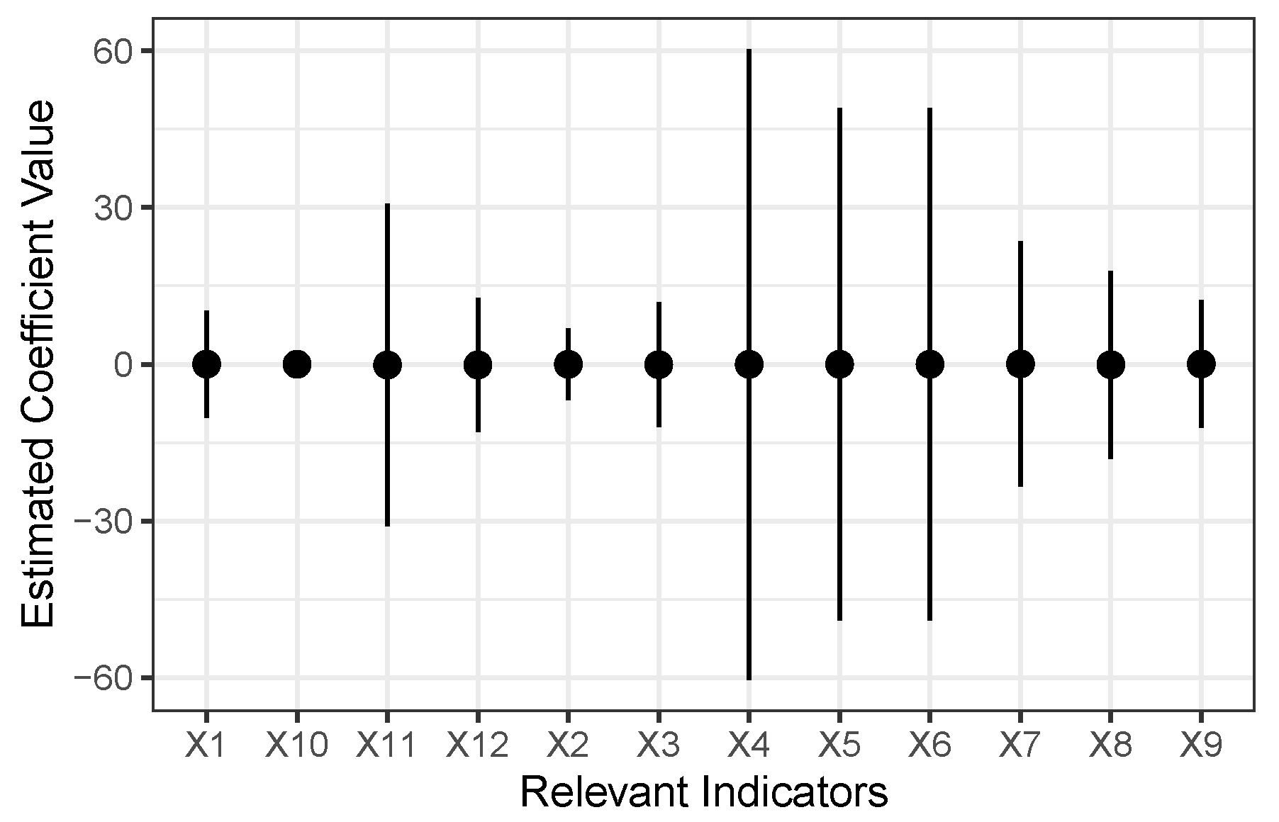
where ${\xi }_i$ is the spatial component, ${\varphi }_t$ and ${\gamma }_t$ represent unstructured and structured temporal effects, respectively and ${\delta }_{it}$ represents the space-time interaction term. $\mathit{\beta }={({\beta }_1,{\beta }_2,\dots ,{\beta }_p)}^{{}^{\prime }}$ represents the vector of covariate coefficients; $X_i={(x_{i1},x_{i2},\dots ,x_{ip})}^{{}^{\prime }}$ is the COVID-19 relevant covariate data vector to be discussed in Section 3.2. Denoting the vector of spatial effects by $\mathit{\xi }={({\xi }_i,\dots ,{\xi }_n)}^{{}^{\prime }}$, the Leroux CAR specification can be defined as:

$$\begin{array}{c}\hfill \mathit{\xi }\sim N(0,{\mathit{D}}_{\mathit{s}}({\sigma }_s^2,{\lambda }_s)),{\mathit{D}}_{\mathit{s}}={\sigma }_s^2{({\lambda }_s{\mathit{R}}_{\mathit{s}}+(1-{\lambda }_s){\mathit{I}}_{\mathit{s}})}^{-1}\end{array}$$

(2)

Table 1. Specification of the Four Types of Spatial–temporal Interaction.

Type of Spatial–Temporal Interaction	${\mathit{R}}_{\mathit{\delta }}$
I	$I_s⨂I_t$
II	$I_s⨂R_t$
III	$R_s⨂I_t$
IV	$R_s⨂R_t$

The term ${\gamma }_t$ represents the temporally structured effect where random walk of first order (RW1) is considered. That is $\mathit{\gamma }={({\gamma }_1,\dots ,{\gamma }_t)}^{{}^{\prime }}\sim N(\mathbf{0},{\sigma }_{\gamma }^2{\mathit{R}}_t^{-})$, where ${\sigma }_{\gamma }^2$ is the variance component. Gaussian distribution is chosen for unstructured temporal effect ${\varphi }_t$: ${\varphi }_t\sim N(0,{\sigma }_{\varphi }^2)$.

The identity matrices $I_s\left(I_t\right)$ correspond to the unstructured spatial (temporal) effect respectively, whereas $R_t\left(R_s\right)$ represent matrices that correspond to a specific structured temporal (spatial) effect (RW1) as follows. We also consider the random walk of second order (RW2), but the performance is not good as the one when RW1 is included.

$$R_t=\left[\begin{array}{ccccccccc}1& -1& & & & & & & \\ -1& 2& -1& & & & & & \\ & -1& 2& -1& & & & \\ & & -1& 2& -1& & & \\ & & \ddots & \ddots & \ddots & \ddots & \ddots & & & \\ & & & -1& 2& -1& 0& 0& \\ & & & & & -1& 2& -1& 0\\ & & & & & & -1& 2& -1\\ & & & & & & & -1& 1\end{array}\right]$$

$$R_s=\left\{\begin{array}{cc}{\displaystyle \sum _{k\sim i}}{\omega }_{ki},\hfill & i=k\hfill \\ -1,\hfill & i\sim k\hfill \\ 0,\hfill & otherwise\hfill \end{array}\right.$$

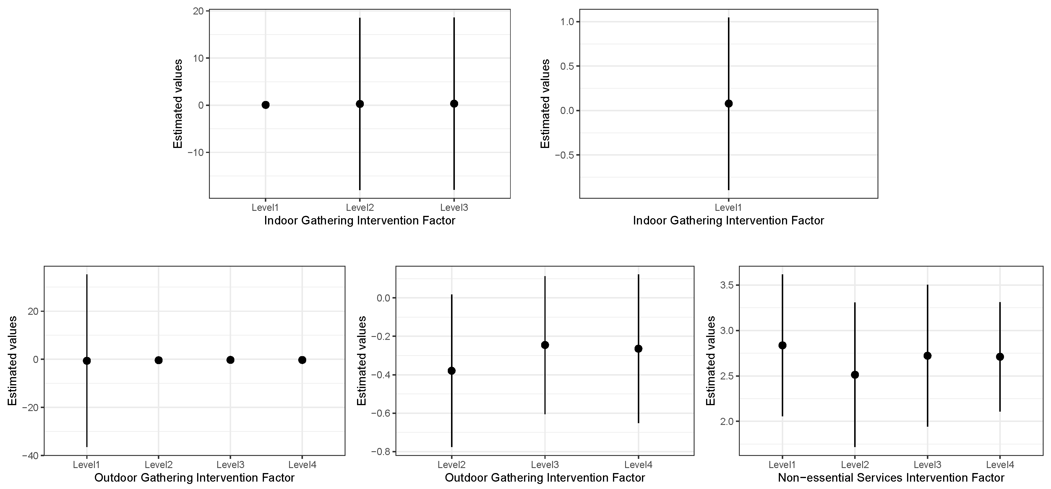
where ${\omega }_{ki}=1$ if areas k and i are sharing the same boundary. As discussed in Section 2, there are three different policies selected and categorized as three different variables. The variable Indoor Gathering (IG) will be defined as 3 indicator variables according to the different restrictions level: $I{G}_i=1$ if the i-th level gathering restriction was in place, and 0 otherwise, for $i=1,2,3$. The variables Outdoor Gathering (OG) and Non-essential service also can be defined as indicator variables according to the different restrictions level. These variables can also be included into the Bayesian Spatial–temporal Models to determine how they influence the infected risk:

$$\begin{array}{cc}\hfill & y_{it}\sim Poisson\left({\mu }_{it}\right)\hfill \\ \hfill & log\left({\mu }_{it}\right)=log\left(e_i\right)+{\theta }_{it}\hfill \\ \hfill & {\theta }_{it}=\alpha +\mathit{\beta }{}^{\prime }{X}_i+\sum _{j=1}^3{\beta }_{IGj}{G}_{ijt}+\sum _{j=1}^4{\beta }_{OGj}{G}_{ijt}+\sum _{j=1}^4{\beta }_{Ej}{E}_{ijt}+{\xi }_i+{\gamma }_t+{\varphi }_t+{\delta }_{it}\hfill \\ \hfill & \mathit{\xi }\sim N(0,{\mathit{D}}_{\mathit{s}}({\sigma }_s^2,{\lambda }_s)),{\mathit{D}}_{\mathit{s}}={\sigma }_s^2{({\lambda }_s{\mathit{R}}_{\mathit{s}}+(1-{\lambda }_s){\mathit{I}}_{\mathit{s}})}^{-1}\hfill \\ \hfill & {\gamma }_t|{\gamma }_{t-1}\sim N({\gamma }_{t-1},{\sigma }_{\gamma }^2),{\varphi }_t\sim N(0,{\sigma }_{\varphi }^2)\hfill \\ \hfill & \mathit{\delta }\sim N(0,{\sigma }_{\delta }^2{R}_{\delta }),\mathit{\delta }=({\delta }_{11},\dots ,{\delta }_{nT})\hfill \end{array}$$

(3)

The spatial component distribution can also be expressed as ${\xi }_i|{\xi }_{k\ne i}\sim N(\frac{{\lambda }_s}{1-{\lambda }_s+{\lambda }_s{m}_i}{\sum }_{k\sim i}{\xi }_i,\frac{{\sigma }_s^2}{1-{\lambda }_s+{\lambda }_s{m}_i})$ Where ${\lambda }_s$ is a spatial smoothing parameter taking values between 0 and 1, ${\mathit{I}}_{\mathit{s}}$ is an identity matrix of dimension $n\times n$ and ${\mathit{R}}_{\mathit{s}}$ is the spatial neighboring matrix which corresponds to the structured spatial effect. $m_i$ is the number of neighbors around area i. That is $m_i={\sum }_{k\sim i}{\omega }_{ki}$, with $k\sim i$ referring to neighbor regions i and j sharing a common boundary. When ${\lambda }_s=0$, the Leroux CAR reduces to $\mathit{\xi }\sim N(0,{\sigma }_s^2{\mathit{I}}_{\mathit{n}})$, and when ${\lambda }_s=1$, it is $\mathit{\xi }\sim N(0,{\sigma }_s^2{{\mathit{R}}_{\mathit{s}}}^{-})$. The unstructured temporal effect ${\mathit{\varphi }}_{\mathit{t}}$ is modelled as independent and identical normal distribution. That is, $\mathit{\varphi }\sim N(\mathbf{0},{\sigma }_{\varphi }^2{\mathit{I}}_{\mathit{t}})$. For the structured temporal effect ${\mathit{\gamma }}_{\mathit{t}}$, a random walk of first order is considered. That is $\mathit{\gamma }\sim N(\mathbf{0},{\sigma }_{\gamma }^2{{\mathit{R}}_{\mathit{t}}}^{-})$. The interaction terms $\mathit{\delta }={({\delta }_{11},\dots ,{\delta }_{nT})}^{{}^{\prime }}$ are assumed to be a normal distribution as $N(\mathbf{0},{\sigma }_{\delta }^2{\mathit{R}}_{\mathit{\delta }})$, where ${\sigma }_{\delta }^2$ is the hyper-parameter and ${\mathit{R}}_{\mathit{\delta }}$ is the matrix given by the Kronecker product of the corresponding matrices of the effects [27]. This model can be built in R-INLA with generic1 option [12].

3.2. Integrated Nested Laplace Approximation (INLA)

The model in Section 3.1 can be fitted using the following modelling framework:

$$\begin{array}{cc}\hfill & y_{it}\sim \mathrm{Poisson}\left({\mu }_{it}\right)\hfill \\ \hfill & log\left(\frac{{\mu }_{it}}{e_i}\right)=\alpha +\sum _{m=1}^M{\beta }_m{x}_{im}+\sum _{q=1}^Q{\eta }_q{x}_{itq}^{*}+\sum _{l=1}^L{f}_l(⬝)+h\left({\delta }_{it}\right)\hfill \end{array}$$

(4)

where $\alpha$ is a scalar representing the intercept; the coefficients $\mathit{\beta }={({\beta }_1,\dots ,{\beta }_M)}^{{}^{\prime }}$ and $\mathit{\eta }={({\eta }_1,\dots ,{\eta }_Q)}^{{}^{\prime }}$ quantify the effect of additional relevant covariates $X_i={(x_{i1},\dots ,x_{iM})}^{{}^{\prime }}$ and policy covariates $X_{it}^{*}={(x_{it1}^{*},\dots ,x_{itQ}^{*})}^{{}^{\prime }}$ on the response; and $\mathit{f}=\{f_1(⬝),\dots ,f_L(⬝)\}$ are a set of functions defined in terms of spatially, temporally correlated effects and ${\delta }_{it}$ is the interaction space and time effect; $\mathit{y}={(y_{11},\dots ,y_{NT})}^{{}^{\prime }}$ represents the vector of biweekly COVID-19 infected cases, N is the number of public health units in Ontario and T is the number of biweeks observed. For the Bayesian Spatial–temporal model in Section 3.1, we identify $f_1(⬝)\sim N(0,{\mathit{D}}_{\mathit{s}}({\sigma }_s^2,{\lambda }_s))$, $f_2(⬝)\sim N(\mathbf{0},{\sigma }_{\gamma }^2{{\mathit{R}}_{\mathit{t}}}^{-})$, $f_3(⬝)\sim N(\mathbf{0},{\sigma }_{\varphi }^2{\mathit{I}}_{\mathit{t}})$ and $h(⬝)\sim N(\mathbf{0},{\sigma }_{\delta }^2{\mathit{R}}_{\mathit{\delta }})$. Upon varying the form of the functions $f_l(⬝)$, this formulation can accommodate a wide range of models, from standard and hierarchical regression, to spatial and spatial–temporal models [16,28].

The spatial–temporal models fitted into this framework are built as Bayesian hierarchical models with three stages [24]. The first stage is the model for infected cases given parameters $p\left(\mathit{y}\right|\mathit{\theta })$, where $\mathit{y}$ denotes the observed cases. The second stage is the model on each parameter $p\left(\mathit{\theta }\right|\mathit{\psi })$. The third stage is the prior on the hyper-parameters $p\left(\mathit{\psi }\right)$. Note: $\mathit{\theta }={(\alpha ,\mathit{\beta },\mathit{\eta },\mathit{\xi },\mathit{\varphi },\mathit{\gamma },\mathit{\delta })}^{{}^{\prime }}$ and $\mathit{\psi }={({\psi }_1,{\psi }_2,\dots ,{\psi }_K)}^{{}^{\prime }}$.

The objectives of the Bayesian computation consist of calculating the marginal posterior distributions for each parameter and hyper-parameter:

$$\begin{array}{cc}\hfill p\left({\theta }_i\right|\mathit{y})& =\int p\left(\mathit{\psi }\right|\mathit{y})p\left({\theta }_i\right|\mathit{\psi },\mathit{y})d\mathit{\psi }\hfill \\ \hfill p\left({\psi }_k\right|\mathit{y})& =\int p\left(\mathit{\psi }\right|\mathit{y})d{\mathit{\psi }}_{-\mathit{k}}\hfill \end{array}$$

(5)

${\mathit{\psi }}_{-\mathit{k}}$ represents the vector but no kth component. The first item we need compute is an approximation to the posterior marginal distribution of the hyper-parameters as

$$p\left(\mathit{\psi }\right|\mathit{y})\propto \frac{p\left(\mathit{\psi }\right)p\left(\mathit{\theta }\right|\mathit{\psi }\left)p\right(\mathit{y}\left|\mathit{\theta }\right)}{p\left(\mathit{\theta }\right|\mathit{\psi },\mathit{y})}\approx {\left.\frac{p\left(\mathit{\psi }\right)p\left(\mathit{\theta }\right|\mathit{\psi }\left)p\right(\mathit{y}\left|\mathit{\theta }\right)}{\tilde{p}\left(\mathit{\theta }\right|\mathit{\psi },\mathit{y})}\right|}_{\mathit{\theta }={\mathit{\theta }}^{*}\left(\mathit{\psi }\right)}=:\tilde{p}\left(\mathit{\psi }\right|\mathit{y})$$

(6)

Next, $p\left({\theta }_i\right|\mathit{\psi },\mathit{y})$ is needed to be approximated, and it is possible to re-express the vector of parameters as $\mathit{\theta }=({\theta }_i,{\mathit{\theta }}_{-i})$ and make use of the Laplace approximation again to obtain:

$$p\left({\theta }_i\right|\mathit{\psi },\mathit{y})\propto \frac{p\left(\mathit{\psi }\right)p\left(\mathit{\theta }\right|\mathit{\psi }\left)p\right(\mathit{y}\left|\mathit{\theta }\right)}{p\left({\mathit{\theta }}_{-i}\right|{\theta }_i,\mathit{\psi },\mathit{y})}\approx {\left.\frac{p\left(\mathit{\psi }\right)p\left(\mathit{\theta }\right|\mathit{\psi }\left)p\right(\mathit{y}\left|\mathit{\theta }\right)}{\tilde{p}\left({\mathit{\theta }}_{-i}\right|{\theta }_i,\mathit{\psi },\mathit{y})}\right|}_{{\mathit{\theta }}_{-i}={\mathit{\theta }}_{-i}^{*}({\theta }_i,\mathit{\psi })}=:\tilde{p}\left({\theta }_i\right|\mathit{\psi },\mathit{y})$$

(7)

Here, $\tilde{p}\left({\theta }_i\right|\mathit{\psi },\mathit{y})$ represents the Gaussian approximation to $p\left({\theta }_i\right|\mathit{\psi },\mathit{y})$ and ${\mathit{\theta }}_{-i}={\mathit{\theta }}_{-i}^{*}({\theta }_i,\mathit{\psi })$ is its mode. The approximation typically works very well, but it can be very expensive in computational terms. Rue et al. [16] proposed the Simplified Laplace Approximation. Numerical integration is used to evaluate the conditional posteriors $\tilde{p}\left({\theta }_i\right|{\psi }_k,\mathit{y})$ and corresponding marginal posteriors $\tilde{p}\left({\theta }_i\right|\mathit{y})$ on a grid of selected values for ${\theta }_i$.

$$\tilde{p}\left({\theta }_i\right|\mathit{y})\approx \sum _{k=1}^K\tilde{p}\left({\theta }_i\right|{\psi }_k,\mathit{y})\tilde{p}\left({\psi }_k\right|\mathit{y}){▵}_k$$

(8)

3.3. Area-to-Point (ATP) and Area-to-Area (ATA) Poisson Kriging

We assume $v_i(i=1,\dots ,34)$ represents the public health unit in Ontario and u is the point location centered in each 15 × 15 square cell we partitioned and we use $s,s^{{}^{\prime }}$ to index different points in units $i,j$. The 15 × 15 cells are chosen since it has better performance after we tried different cells, 5 × 5, 8 × 8, and 10 × 10, 15 × 15. The observed age-adjusted bi-weekly COVID-19 infection rate is then denoted as $z\left(v_i\right)=S\left(v_i\right)/n\left(v_i\right)$, where $n\left(v_i\right)$ is the population size in public health unit i. At each unit i, the corresponding infected cases $S\left(v_i\right)$ can be assumed to follow a conditional Poisson distribution given local risk $R\left(v_i\right)$:

$$S\left(v_i\right)|R\left(v_i\right)\sim \mathrm{Poisson}\left(n\left(v_i\right)R\left(v_i\right)\right)$$

(9)

Therefore, these cases are spatially correlated in either the population sizes or in the risks. The risk variable $R\left(v_i\right)$ itself can be distributed as an unknown distribution with mean value m, variance value ${\sigma }_R^2$ and variance function $C_R(v_i,v_j)$ [5]. It is not realistic to just assume each unit $v_i$ to its geographic centroid because the distances between these public health units are large. Also, they have different shapes and sizes. The spatial correlation of each unit needs to be considered. Area-to-Area (ATA) Kriging is used to predict the areal risks and we assume areal supports are disjointed [29]. The estimated areal risk value $r\left(v_{\alpha }\right)$ in an arbitrary unit $\alpha$ thus can be expressed as a weighted linear combination of the K neighboring available areal infection rates:

$${\widehat{r}}_{PK}\left(v_{\alpha }\right)=\sum _{i=1}^K{\lambda }_i\left(v_{\alpha }\right)z\left(v_i\right)$$

(10)

where $z\left(v_i\right)$ is the biweekly age-adjusted infection rate in each public health unit i. The areal weights ${\lambda }_i\left(v_{\alpha }\right)$ can be calculated through the following system:

$$\begin{array}{cc}\hfill & \sum _{j=1}^K{\lambda }_j\left(v_{\alpha }\right)[{\overline{C}}_R(v_i,v_j)+{\delta }_{ij}\frac{m*}{n\left(v_i\right)}]+\mu \left(v_{\alpha }\right)={\overline{C}}_R(v_i,v_{\alpha })i=1,\dots ,K\hfill \\ \hfill & \sum _{j=1}^K{\lambda }_j\left(v_{\alpha }\right)=1\hfill \end{array}$$

(11)

where ${\overline{C}}_R(v_i,v_j)=\mathrm{Cov}\{z\left(v_i\right),z\left(v_j\right)\}$. The areal covariances are approximated by averaging point-to-point covariances $C(u_s,u_{s^{\prime }})$ calculated between any two points which can discretize the units $v_i$ and $v_j$:

$${\overline{C}}_R(v_i,v_j)=\frac{1}{{\sum }_{s=1}^{P_i}{\sum }_{s^{\prime }=1}^{P_j}{w}_{s{s}^{\prime }}}\sum _{s=1}^{P_i}\sum _{s^{\prime }=1}^{P_j}{w}_{s{s}^{\prime }}C(u_s,u_{s^{\prime }})$$

(12)

where $P_i$ and $P_j$ represent the number of points discretizing the corresponding two areas $v_i$ and $v_j$. The weights $w_{s{s}^{\prime }}$ are calculated as the product of population sizes in each 15 km × 15 km square cell centered on the points $u_s$ and $u_{s^{\prime }}$:$w_{s{s}^{\prime }}=n\left(u_s\right)\times n\left(u_{s^{\prime }}\right)$. Therefore, the sum of population size in each cell within unit is equal to the population size in each unit: $n\left(v_i\right)={\sum }_{s=1}^{P_i}n\left(u_s\right)$ and $n\left(v_j\right)={\sum }_{s=1}^{P_j}n\left(u_{s^{\prime }}\right)$. The kriging variance for estimated areal risk in unit $\alpha$ is computed as:

$${\sigma }_{PK}^2\left(v_{\alpha }\right)={\overline{C}}_R(v_{\alpha },v_{\alpha })-\sum _{i=1}^K{\lambda }_i\left(v_{\alpha }\right){\overline{C}}_R(v_i,v_{\alpha })-\mu \left(v_{\alpha }\right)$$

(13)

where ${\overline{C}}_R(v_{\alpha },v_{\alpha })$ is the covariance within the same area $\alpha$:

$${\overline{C}}_R(v_{\alpha },v_{\alpha })=\frac{1}{n^2\left(v_{\alpha }\right)}[\sum _{s=1}^{P_{\alpha }}{n}^2\left(u_s\right)C\left(\mathbf{0}\right)+\sum _{s=1}^{P_{\alpha }}\sum _{s^{\prime }=1}^{P_{\alpha }}{w}_{s{s}^{\prime }}C(u_s,u_{s^{\prime }}){\delta }_{s{s}^{\prime }}(s\ne s^{\prime })]$$

(14)

and ${\delta }_{s{s}^{\prime }}(s\ne s^{\prime })$ is the indicator function. Alternatively, kriging may be used to predict a value $r\left(u_s\right)$ also in use of K neighboring areal infection rates $\{z\left(v_i\right),i=1,\dots ,K\}$ [29]. The predicted point risk ${\widehat{r}}_{PK}\left(u_s\right)$ can also be expressed as a weighted linear combination. Here, $u_s$ represents the point location whose risk value will be estimated.

$${\widehat{r}}_{PK}\left(u_s\right)=\sum _{i=1}^K{\lambda }_i\left(u_s\right)z\left(v_i\right)$$

(15)

The system of linear equations that is used to compute the kriging weights is similar to the one used for calculating weights in the ATA kriging method. However, the area-to-area covariances ${\overline{C}}_R(v_i,v_{\alpha })$ on the right-side of first equation in (11) are replaced by area-to-point covariances ${\overline{C}}_R(v_i,u_s)$ approximated as follows:

$${\overline{C}}_R(v_i,u_s)=\frac{1}{{\sum }_{s^{\prime }=1}^{P_i}{w}_{s^{\prime }s}}\sum _{s^{\prime }=1}^{P_i}{w}_{s^{\prime }s}C(u_{s^{\prime }},u_s)$$

(16)

where $P_i$ is the number of points in area $v_i$. The area-to-point kriging variance is estimated as:

$${\sigma }_{PK}^2\left(u_s\right)=C_R\left(0\right)-\sum _{i=1}^K{\lambda }_i\left(u_s\right){\overline{C}}_R(v_i,u_s)-\mu \left(u_s\right)$$

(17)

In order to solve systems of equations, the covariance $C(u_s,u_{s^{\prime }})$ or equivalently the point-to-point semivariogram $\gamma (u_s,u_{s^{\prime }})$ is needed. It can be computed through the relationship [30,31]:

$${\gamma }_v\left(\mathbf{h}\right)=\overline{\gamma }(v,v_{\mathbf{h}})-{\overline{\gamma }}_{\mathbf{h}}(v,v)$$

(18)

here, $\mathbf{h}$ is the vector of distances. The second term on the right side is calculated by averaging point-to-point semivariogram values in the same unit for any pairs of units separated by given distances $\mathbf{h}$:

$${\overline{\gamma }}_{\mathbf{h}}(v,v)=\frac{1}{2N\left(\mathbf{h}\right)}\sum _{i=1}^{N\left(\mathbf{h}\right)}[\frac{1}{P_i^2}\sum _{s=1}^{P_i}\sum _{s^{\prime }=1}^{P_i}\gamma (u_s,u_{s^{\prime }})+\frac{1}{P_{i+\mathbf{h}}^2}\sum _{s=1}^{P_{i+\mathbf{h}}}\sum _{s^{\prime }=1}^{P_{i+\mathbf{h}}}\gamma (u_s,u_{s^{\prime }})],$$

(19)

where $P_i$ and $P_{i+\mathbf{h}}$ are the number of points in units $v_i$ and $v_{i+\mathbf{h}}$ respectively, $N\left(\mathbf{h}\right)$ is the number of pairs of units given distances $\mathbf{h}$. The area-to-area semivariogram value, $\overline{\gamma }(v,v_{\mathbf{h}})$, is also estimated through point-to-point semivariograms:

$$\overline{\gamma }(v,v_{\mathbf{h}})=\frac{1}{N\left(\mathbf{h}\right)}\sum _{i=1}^{N\left(\mathbf{h}\right)}\frac{1}{P_i{P}_{i+\mathbf{h}}}\sum _{s=1}^{P_i}\sum _{s^{\prime }=1}^{P_{i+\mathbf{h}}}\gamma (u_s,u_{s^{\prime }})$$

(20)

The estimating point-support semivariogram procedure starts with the choice of an initial one ${\gamma }^{\left(0\right)}\left(\mathbf{h}\right)$ and the estimation is best tackled using an iterative procedure until the difference between theoretically regularized areal semivariogram and experimental areal semivariogram is small [32,33].

4. Applications of Methodologies

4.1. Model Selection

Following the discussion in Section 3.1, there are 4 models proposed as indicated in Table 2:

Table 2. Model Specification.

Models	Components
Model 1	$\alpha +{\sum }_{j=1}^3{\beta }_{IGj}{G}_{ijt}+{\sum }_{j=1}^4{\beta }_{Ej}{E}_{ijt}+{\sum }_{j=1}^4{\beta }_{OGj}{B}_{ijt}+\mathit{\beta }{X}_i+{\xi }_i+{\gamma }_t+{\varphi }_t+{\delta }_{it}$ (Type I)
Model 2	$\alpha +{\sum }_{j=1}^3{\beta }_{IGj}{G}_{ijt}+{\sum }_{j=1}^4{\beta }_{Ej}{E}_{ijt}+{\sum }_{j=1}^4{\beta }_{OGj}{B}_{ijt}+\mathit{\beta }{X}_i+{\xi }_i+{\gamma }_t+{\varphi }_t+{\delta }_{it}$ (Type II)
Model 3	$\alpha +{\sum }_{j=1}^3{\beta }_{IGj}{G}_{ijt}+{\sum }_{j=1}^4{\beta }_{Ej}{E}_{ijt}+{\sum }_{j=1}^4{\beta }_{OGj}{B}_{ijt}+\mathit{\beta }{X}_i+{\xi }_i+{\gamma }_t+{\varphi }_t+{\delta }_{it}$ (Type III)
Model 4	$\alpha +{\sum }_{j=1}^3{\beta }_{IGj}{G}_{ijt}+{\sum }_{j=1}^4{\beta }_{Ej}{E}_{ijt}+{\sum }_{j=1}^4{\beta }_{OGj}{B}_{ijt}+\mathit{\beta }{X}_i+{\xi }_i+{\gamma }_t+{\varphi }_t+{\delta }_{it}$ (Type IV)

Here $X_i$ represents the vector of covariates discussed in Section 2. The models are assessed using the Deviance Information Criterion (DIC) as shown in Table 3 with lower values indicating a better fit [34]. The criterion takes into account the goodness-of-fit as well as a penalty term that is based on the complexity of the model via the estimated effective number of parameters. The DIC is defined as: $DIC=D\left(\widehat{\mathit{\theta }},\widehat{\mathit{\psi }}\right)+2p_D$. The Watanabe-Akaike information criterion (WAIC), also known as widely applicable Bayesian information criterion, is similar to the DIC but the effective number of parameters is computed in a different way [35,36]. Table 3 shows the DIC value and WAIC values for the different models under RW1. We have grouped together similar models with and without the Leroux specification for appropriate comparisons. The model with better performance will be chosen accordingly.

Table 3. DIC and WAIC Values under RW1.

Models	BYM Specification		Leroux CAR Specification
	DIC	WAIC	DIC	WAIC
Type I Interaction	8434.35	8211.21	8454.02	8361.58
Type II Interaction	8410.87	8266.66	8392.16	8247.07
Type III Interaction	8448.85	8239.20	8432.59	8220.86
Type IV Interaction	8442.71	8331.01	8423.18	8200.98

Bold faced values in the table indicate that Type II Interaction has a relatively better performance.

We also considered models with RW2 (second order of random walk). But Using the DIC criterion, models with RW1 structured temporal effect show better performance. It is seen that the model under Type II Interaction has the lowest DIC values when considering Leroux CAR specification for spatial component. In the following sections, we discuss the effects of the various coefficients in these models.

4.2. Covariates Effect

In Section 4.1, we evaluated all of the models. Regarding the effect of each covariate on the spread of COVID-2019, the summary of each coefficient on these indicators discussed in Section 2 is reflected in Figure 1:

Figure 1. Summary of the Estimates Obtained for the Coefficients Associated with Indicators for Model 2.

Figure 1 shows the range value of each coefficient from (mean-sd) to (mean+sd). It can be seen that almost all these covariates do not have significant associations with infected risk.

4.3. Policy Effect

For the policy analysis, regarding the effect of each intervention factor on the spread of COVID-2019, the summay of each coefficient on the intervention factors is reflected in Figure 2:

Figure 2. Summary of the Estimates Obtained for the Intervention Factors Associated with Covariates for Model 2.

Figure 2 also shows the same range value from (mean − sd) to (mean + sd) as in Figure 1. It can be seen from Figure 2 that the levels 1–4 in Non-essential Services Intervention Factor are significant, and the levels 2–4 in Outdoor Gathering Intervention Factor could be significant as well.

4.4. Spatial–Temporal Effect

The spatial–temporal effects help us to understand how the pandemic spreads over time and space in Ontario. The infected risks in each public health unit can be calculated by exponentiating the parameters for space, time, space-time, relevant additional, or government interaction, as $exp\left({\theta }_{it}\right)$. From Figure 3, we can see some regions in Southern Ontario with higher infection rates at some time point. At the beginning, the risks in the Northern area are relatively small, but they increase after January 2021, when the second wave started. Since the third wave, the infected current cases in Northern Ontario are more than in Southern Ontario.

Figure 3. Evolution of the Infected Risks at the Public Health Unit Level (Model 2).

5. Discussion and Conclusions

5.1. Prediction Performance on Bayesian Methods

We examined the prediction performance of our proposed models. We take the data until time $T^{*}$ and predict the infected risk within q bi-weeks ahead, i.e., $y_{it}^{*}$ for $t=T^{*}+1$, …,$T^{*}+q$. The prediction performance is evaluated using the absolute mean error of prediction (AMEP) given by

$$AMEP=\frac{1}{Iq}\sum _{T^{*}+1}^{T^{*}+q}\sum _{i=1}^I\parallel exp(\widehat{{\theta }_{it}}-exp\left({\theta }_{it}\right)\parallel$$

The results for q = 1 and q = 2, i.e., predicting 1 and 2 time periods ahead, are given in Table 4 and Table 5 respectively. We choose $T^{*}=30$ or $T^{*}=31$ to give a sufficient observed data for prediction. For each $T^{*}$ and q, the AMEP is reported for the Model 1–4. Model 2 (corresponding to Type II interaction) performs better by giving the smaller AMEP value when $T^{*}=30$ and q = 2. Model 3 (corresponding to Type III interaction ) gives the smallest AMEP value when $T^{*}=31$ and q = 1. Generally, Model 2 (Type II interaction) has a better performance when doing longer-term predictions. Prediction performance with Leroux CAR specification for spatial component is not as good as BYM specification’s.

Table 4. Results of 1-biweek Ahead Prediction for Models 1–4.

Models	BYM Specification	Leroux CAR Specification
Type I	63.3313	63.7554
Type II	30.8323	59.9799
Type III	27.5105	78.0949
Type IV	76.0943	81.1585

Table 5. Results of 2-biweeks Ahead Prediction for Models 1–4.

Models	BYM Specification	Leroux CAR Specification
Type I	84.7722	81.8366
Type II	17.7088	53.0448
Type III	27.2464	113.6560
Type IV	75.5361	76.2468

5.2. Estimation Performance on Poisson Kriging Models

We examine the estimation performance of Area-to-area (ATA) Poisson Kriging Model in use of Mean Absolute Error of Estimation (MAEE). Table 6 shows the result as follows:

$$MAEE=\frac{1}{I}\sum _{i=1}^{34}(\parallel {\widehat{r}}_{PK}\left(v_{\alpha }\right)-z\left({\mathbf{v}}_{\alpha }\right)\parallel )$$

Table 6. Estimation Performance with ATA Poisson Kriging Model.

Date	MAEE	Date	MAEE	Date	MAEE	Date	MAEE
31 March 2020	9.1583	14 April 2020	27.5731	30 November 2020	45.2185	14 December 2020	51.2377
30 April 2020	18.1985	14 May 2020	9.9172	31 December 2020	81.5218	14 January 2021	75.8301
31 May 2020	14.4495	14 June 2020	14.0699	31 January 2021	56.2901	14 February 2021	27.8829
30 June 2020	10.9806	14 July 2020	4.9548	28 February 2021	37.8338	14 March 2021	54.8017
31 July 2020	9.8015	14 August 2020	9.1887	31 March 2021	73.2944	14 April 2021	76.0162
31 August 2020	5.9091	14 September 2020	6.1367	30 April 2021	72.6466	14 May 2021	78.9172
30 September 2020	12.4405	14 October 2020	15.2833	31 May 2021	95.2153	14 June 2021	73.0008
31 October 2020	23.9789	14 November 2020	31.6626	31 June 2021	49.7580	-	-

It can be seen from Table 6 that generally the estimation performance is good. The range in point support semivariograms from ATP Poisson Kriging Model can show the spatial clustering feature of COVID-19 spreading reliably. Table 7 shows different ranges in each time period:

Table 7. Ranges in Point Support Semivariograms.

Date	Range	Date	Range	Date	Range	Date	Range
31 March 2020	75.4 km	14 April 2020	114.9 km	30 November 2020	44.0 km	14 December 2020	73.6 km
30 April 2020	28.0 km	14 May 2020	123.7 km	31 December 2020	151.0 km	14 January 2021	136 km
31 May 2020	240.0 km	14 June 2020	108.4 km	31 January 2021	106.0 km	14 February 2020	101.6 km
30 June 2020	126.8 km	14 July 2020	80.5 km	28 February 2021	151 km	14 March 2021	247.5 km
31 July 2020	116.7 km	14 August 2020	133.8 km	31 March 2021	76 km	14 April 2021	121 km
31 August 2020	102.0 km	14 September 2020	53.0 km	30 April 2021	84.8 km	14 May 2021	84.4 km
30 September 2020	87.6 km	14 October 2020	104.8 km	31 May 2021	355.9 km	14 June 2021	272.2 km
31 October 2020	104.4 km	14 November 2020	72.8 km	30 June 2021	74.3 km	-	-

In the case of semivariogram, for sample points with close distances, the difference in values between points tends to be small. In other words, the semivariance is small. But they are larger as the distances between sample points increase. It also means these point’s risk values are not correlated closely anymore [37]. The range represents the distance at which the model first flattens out. Therefore, range value can represent the spatial clustering feature. It can be seen that the largest range value is 355 km, which means the infected cases are clustered spatially within 355 km at most. Public health office can pay more attention to monitor the infected cases around each hotspot under 355 km.

5.3. Conclusions

Here are some conclusions made based on the previous analysis:

(1)

The Poisson Kriging methods display more clearly the spread of the virus spreads over space. Kriging methods in general produce a smoother surface, which leads to overestimated results at non-hot spot regions. Bayesian Spatial–temporal methods provide a more accurate predictions.

(2)

ATP Poisson Kriging model provides a good thought to downscale areal risk maps into point risk maps given a specific timeframe. The range values from point support semivariograms can be a good reference for government to monitor how the virus spreads around each hotspot at early stage of the pandemic.

(3)

The following government interventions were found to be significant: (a) levels 1–4 in non-essential services are sit-down dining and; (b) levels 2–4 in Outdoor Gathering Intervention.

(4)

The infected risk was nearly 0 over Ontario in March 2020. The second wave and third wave started from November 2020 and April 2021, respectively. At the start, the risks in the Northern area were relatively small, but they increased after January, 2021, when the second wave began. Since the third wave, the increment of infected current cases in Northern Ontario were more than in Southern Ontario.

(5)

The Bayesian Spatial–temporal Model 2 included interactions between unstructured spatial and structured temporal effects, whereas Model 3 included interaction between structured spatial and unstructured temporal effects.The results for short-term prediction were better for both Models.

(6)

The interactive website we developed displays the estimated risk maps by date and model choice: Bayesian Spatial–temporal or Kriging.

(7)

A Shinyapp website https://mujingrui.shinyapps.io/covid19 displays spatial–temporal maps exploiting these models.

References

- Park, H.; Kim, S.H. A study on herd immunity of COVID-19 in South Korea: Using a stochastic economic-epidemiological model. Environ. Resour. Econ. 2020, 76, 665–670. [Google Scholar] [CrossRef]
- Sarkar, K.; Khajanchi, S.; Nieto, J.J. Modeling and forecasting the COVID-19 pandemic in India. Chaos Solit. Fractals 2020, 139, 110049. [Google Scholar] [CrossRef] [PubMed]
- Taboe, H.B.; Salako, K.V.; Tison, J.M.; Ngonghala, C.N.; Kakaï, R.G. Predicting COVID-19 spread in the face of control measures in West Africa. Math. Biosci. 2020, 328, 108431. [Google Scholar] [CrossRef] [PubMed]
- Zhao, Z.; Li, X.; Liu, F.; Zhu, G.; Ma, C.; Wang, L. Prediction of the COVID-19 spread in African countries and implications for prevention and control: A case study in South Africa, Egypt, Algeria, Nigeria, Senegal and Kenya. Sci. Total Environ. 2020, 729, 138959. [Google Scholar] [CrossRef]
- Goovaerts, P. Geostatistical analysis of disease data: Accounting for spatial support and population density in the isopleth mapping of cancer mortality risk using area-to-point Poisson kriging. Int. J. Health Geogr. 2006, 5, 7. [Google Scholar] [CrossRef]
- Goovaerts, P. Geostatistical analysis of disease data: Estimation of cancer mortality risk from empirical frequencies using Poisson kriging. Int. J. Health Geogr. 2005, 4, 1–31. [Google Scholar] [CrossRef] [PubMed]
- Goovaerts, P. Geostatistical analysis of disease data: Visualization and propagation of spatial uncertainty in cancer mortality risk using Poisson kriging and p-field simulation. Int. J. Health Geogr. 2006, 5, 1–26. [Google Scholar] [CrossRef]
- Besag, J.; York, J.; Mollie, A. Bayesian image restoration with two applications in spatial statistics. Ann. Inst. Stat. Math. 1991, 43, 1–20. [Google Scholar] [CrossRef]
- Best, N.G.; Richardson, S.; Thomson, A. A comparison of Bayesian spatial models for disease mapping. Stat. Methods Med. Res. 2005, 14, 35–59. [Google Scholar] [CrossRef]
- MacNab, Y.C. On Gaussian Markov random fields and Bayesian disease mapping. Stat. Methods Med. Res. 2011, 20, 49–68. [Google Scholar] [CrossRef]
- Martínez-Bello, D.; López-Quílez, A.; Prieto, A.T. Spatiotemporal modeling of relative risk of dengue disease in Colombia. Stoch. Environ. Res. Risk Assess. 2018, 32, 1587–1601. [Google Scholar] [CrossRef]
- Ugarte, M.D.; Adin, A.; Goicoa, T.; Militino, A.F. On fitting spatio-temporal disease mapping models using approximate Bayesian inference. Stat. Methods Med. Res. 2014, 23, 507–530. [Google Scholar] [CrossRef] [PubMed]
- Brooks, S.; Gelman, A.; Jones, G.; Meng, X.L. (Eds.) Handbook of Markov Chain Monte Carlo; CRC Press: Boca Raton, FL, USA, 2011. [Google Scholar]
- Martínez-Bello, D.A.; López-Quílez, A.; Torres Prieto, A. Relative risk estimation of dengue disease at small spatial scale. Int. J. Health Geogr. 2017, 16, 31. [Google Scholar] [CrossRef] [PubMed]
- Robert, C.P.; Casella, G. The Metropolis—Hastings Algorithm. In Monte Carlo Statistical Methods; Springer: New York, NY, USA, 2004; pp. 267–320. [Google Scholar]
- Rue, H.; Martino, S.; Chopin, N. Approximate Bayesian inference for latent Gaussian models by using integrated nested Laplace approximations. J. R. Stat. Soc. Series. B. Stat. Methodol. 2009, 71, 319–392. [Google Scholar] [CrossRef]
- Lee, D. A comparison of conditional autoregressive models used in Bayesian disease mapping. Spat. Spatio-Temporal Epidemiol. 2011, 2, 79–89. [Google Scholar] [CrossRef] [PubMed]
- Leroux, B.G.; Lei, X.; Breslow, N. Estimation of disease rates in small areas: A new mixed model for spatial dependence. In Statistics Models in Epidemiology, the Environment and Clinical Trials; Springer: New York, NY, USA, 2000; pp. 179–191. [Google Scholar]
- Schrödle, B.; Held, L.; Riebler, A.; Danuser, J. Using integrated nested laplace approximations for the evaluation of veterinary surveillance data from Switzerland: A case-study. J. R. Stat. Soc. C Appl. Stat. 2011, 60, 261–279. [Google Scholar] [CrossRef]
- Schrödle, B.; Held, L. Spatio-temporal disease mapping using INLA. Environmetrics 2011, 22, 725–734. [Google Scholar] [CrossRef]
- Briz-Redón, Á. The impact of modelling choices on modelling outcomes: A spatio-temporal study of the association between COVID-19 spread and environmental conditions in Catalonia (Spain). Stoch. Environ. Res. Risk Assess. 2021, 35, 1701–1713. [Google Scholar] [CrossRef]
- Jaya, I.G.N.M.; Folmer, H. Bayesian spatiotemporal forecasting and mapping of COVID-19 risk with application to West Java Province, Indonesia. J. Reg. Sci. 2021, 61, 849–881. [Google Scholar] [CrossRef]
- Jaya, I.G.N.M.; Folmer, H. Spatiotemporal high-resolution prediction and mapping: Methodology and application to dengue disease. J. Geogr. Syst. 2022, 24, 527–581. [Google Scholar] [CrossRef]
- Martins, T.G.; Simpson, D.; Lindgren, F.; Rue, H. Bayesian computing with INLA: New features. Comput. Stat. Data. Anal. 2013, 67, 68–83. [Google Scholar] [CrossRef]
- Knorr-Held, L. Bayesian modelling of inseparable space-time variation in disease risk. Stat. Med. 2000, 19, 2555–2567. [Google Scholar] [CrossRef] [PubMed]
- Schrödle, B.; Held, L. A primer on disease mapping and ecological regression using INLA. Comput. Stat. 2011, 26, 241–258. [Google Scholar] [CrossRef]
- Clayton, D. Generalized linear mixed models. In Markov Chain Monte Carlo in Practice; Gilks, W., Richardson, S., Spiegelhalter, D., Eds.; Chapman and Hall: London, UK, 1996; pp. 275–301. [Google Scholar]
- Blangiardo, M.; Cameletti, M.; Baio, G.; Rue, H. Spatial and spatio-temporal models with R-INLA. Spat. Spatio-Temporal Epidemiol. 2013, 4, 33–49. [Google Scholar] [CrossRef] [PubMed]
- Kyriakidis, P.C. A geostatistical framework for area-to-point spatial interpolation. Geogr. Anal. 2004, 36, 259–289. [Google Scholar] [CrossRef]
- Goovaerts, P. Kriging and Semivariogram Deconvolution in the Presence of Irregular Geographical Units. Math. Geosci. 2008, 40, 101–128. [Google Scholar] [CrossRef]
- Journel, A.G.; Huijbregts, C.J. Mining Geostatistics; Academic Press: London, UK, 1978. [Google Scholar]
- Goovaerts, P.; Gebreab, S. How does Poisson kriging compare to the popular BYM model for mapping disease risks? Int. J. Health Geogr. 2008, 1, 6. [Google Scholar] [CrossRef]
- Molinski, S. Pyinterpolate: Spatial Interpolation in Python for point measurements and aggregated datasets. J. Open Source Softw. 2022, 7, 2869. [Google Scholar] [CrossRef]
- Spiegelhalter, D.J.; Best, N.G.; Carlin, B.P.; Van Der Linde, A. Bayesian measures of model complexity and fit. J. R. Stat. Soc. 2002, 64, 583–639. [Google Scholar] [CrossRef]
- Gelman, A.; Hwang, J.; Vehtari, A. Understanding predictive information criteria for Bayesian models. Stat. Comput. 2014, 24, 997–1016. [Google Scholar] [CrossRef]
- Watanabe, S.; Opper, M. Asymptotic equivalence of Bayes cross validation and widely applicable information criterion in singular learning theory. J. Mach. Learn. Res. 2010, 11. [Google Scholar]
- GISGeography. Semi-Variogram: Nugget, Range and Sill. 2022. Available online: https://gisgeography.com/semi-variogram-nugget-range-sill/ (accessed on 9 November 2022).
Disclaimer/Publisher’s Note: The statements, opinions and data contained in all publications are solely those of the individual author(s) and contributor(s) and not of MDPI and/or the editor(s). MDPI and/or the editor(s) disclaim responsibility for any injury to people or property resulting from any ideas, methods, instructions or products referred to in the content. |
© 2023 by the authors. Licensee MDPI, Basel, Switzerland. This article is an open access article distributed under the terms and conditions of the Creative Commons Attribution (CC BY) license (https://creativecommons.org/licenses/by/4.0/).