Article

Multivariate Forecasting Model for COVID-19 Spread Based on Possible Scenarios in Ecuador

1
Facultad de Ingeniería en Ciencias Agropecuarias y Ambientales, Universidad Técnica del Norte, Av. 17 de Julio 5-21 y Gral. José María Córdova, Ibarra 100105, Ecuador
2
Grupo de Investigación de Ciencias en Red (eCIER), Universidad Técnica del Norte, Av. 17 de Julio 5-21 y Gral. José María Córdova, Ibarra 100105, Ecuador
*
Author to whom correspondence should be addressed.
Mathematics 2023, 11(23), 4721; https://doi.org/10.3390/math11234721
Submission received: 30 August 2023 / Revised: 22 September 2023 / Accepted: 25 September 2023 / Published: 22 November 2023
(This article belongs to the Special Issue Analysis and Control of Nonlinear Dynamical System)

Abstract

:
So far, about 770.1 million confirmed cases of COVID-19 have been counted by August 2023, and around 7 million deaths have been reported from these cases to the World Health Organization. In Ecuador, the first confirmed COVID-19 case was registered on 19 February 2020, and the country’s mortality rate reached 0.43% with 12986 deaths, suggesting the need to establish a mechanism to show the virus spread in advance. This study aims to build a dynamic model adapted to health and socio-environmental variables as a multivariate model to understand the virus expansion among the population. The model is based on Susceptible-Infected-Recovered (SIR), which is a standard model in which the population is divided into six groups with parameters such as susceptible S(t), transit stage E(t), infected I(t), recovered R(t), deceased Me(t), infected asymptomatic Ia(t), infected symptomatic Is(t) and deceased by other causes M(t) to be considered and adapted. The model was validated by using consistent data from Chile and run by inconsistent data from Ecuador. The forecast error was analyzed based on the mean absolute error between real data and model forecast, showing errors within a range from 6.33% to 8.41% for Chile, with confidence a interval of 6.17%, then 3.87% to 4.70% range for Ecuador with a confidence interval of 2.59% until 23rd December 2020 of the database. The model forecasts exponential variations in biosecurity measures, exposed population, and vaccination.

1. Introduction

So far, about 770.1 million confirmed cases of COVID-19 have been counted by August 2023, and around 7 million deaths have been reported from these cases to the World Health Organization [1]. Globally, this disease exhibits a mortality rate ranging from 0.66% to 4.44% [2,3]. Ecuador’s first confirmed COVID-19 case was recorded on 19 February 2020 [4]. On 13th March, the National Emergency Operations Committee (COE in Spanish) assumed its functions and started providing daily updates on the national COVID-19 situation, sharing government data and information [5]. Ecuador’s mortality rate reached 0.43%, with 12,986 deaths [6], prompting the implementation of a color-coded mechanism, including red, yellow, and green restrictions, based on the number of virus-infected individuals, leading to quarantine measures. Numerous models and simulations have been developed to predict and analyze COVID-19, to understand the progression of respiratory diseases, and thus to predict the number of infections or the overall disease burden caused by such diseases in vulnerable populations [7,8,9,10]. Generally, there are two approaches to the analysis of pandemic diseases. One exploits natural variation in the distribution of COVID-19, and others develop a dynamic mathematical model [11]. Several studies have demonstrated the reliability of applying mathematical and statistical methods for the analysis of epidemiological data as long as there is a validation of the applied model [12]. While these models have provided significant insights and guided decisions, several gaps and limitations have been identified such as the initial parameters being steady. Due to the lack of detailed data, many models made initial assumptions about the primary reproduction number (R0), disease duration, and severity [13]. R0 has been calculated since Kermack and McKendric in 1920, who developed their model of malaria transmission inspired by the Ross model [14]. R0 is defined as the average number of people to whom an infected person can spread the virus, i.e., it describes the exponential growth of infection during the first phase of the epidemic [15]. However, this number cannot reflect the time-varying nature of an epidemic, as it is a static quantity that mainly accounts for what happens to the pandemic when public health policies are not adopted [16]. During any epidemic’s initial rapid growth phase, R0 numbers can reach high values due to the small initial sample size, low population awareness of the disease, and lack of health system response to deal with the outbreak [17]. However, high values may also occur due to poor availability of testing or delayed results confirming those infected. Consequently, the rate of growth of cases could be steadily altered due to factors such as the proportions of the population exposed or even because the number of cases exceeds the capacity of the system to count them. These difficulties typical of disease and health systems inevitably lead to changes in R0 values [18].
On the other hand, R0 can be modeled within SIRS models (a generic epidemiological model of an infectious disease transmission through individuals passing through the states: susceptible, infectious, recovered, and susceptible) using dynamic factors such as infection rate, recovery rate, growth assumptions of a linear system, and the probability of infection [17,19]. For this purpose, the universe of disease growth data in a specific population is used as a reference. The number can also be calculated using as a reference the mean and standard deviation according to confirmed cases and reporting dates [20], estimating the maximum likelihood using the serial interval distribution of the gamma distribution [21], or maximum likelihood elimination methods with bias correction obtained from chain binomial models [22]. The methods used for this value range from specific distributions for the daily case volume to stochastic models and include statistical inference of transmission chains down to minimum values [16]. By calculating the R0 value in dynamic models, there is a more realistic estimation of the disease’s growth, transmission, and spread in scenarios where the health system has few tools for disease containment and where the population has not yet achieved immunity [16]. Therefore, in the present investigation, a dynamic model was developed that allowed differential equations to identify the relationships between infected cases and the factors that influence their transmission and recovery, considering several scenarios that contemplated 25%, 50%, and 75% exposure in the population. Some studies have shown that the spread of contagious diseases is influenced by socioeconomic or cultural factors that establish the population’s exposure levels [23,24,25]. In this study, factors such as social, cultural, or economic that drove this behavior were not evaluated. Instead, the simulation was based on the exposed population’s conditions related to biosafety measures such as hand washing or face mask use. It was applied iterative methods to COVID-19 time series data to uncover the dynamic models that govern the epidemic patterns of pandemic behavior. Thus, a dynamic mathematical model was addressed to forecast the number of cases based on the rate of infection and recovery, where the R0 number is a key factor. One advantage of this research is that a global model of the early stages of the pandemic was created that can be adapted to any population if there is sufficient temporal information on the infection. Another advantage is that the approach overcomes the problem of heterogeneity because the System Dynamics Models assume that a population within one compartment is homogenous [26,27]. Finally, a relevant benefit is that the information could empower governments to make informed decisions based on scientific predictions and estimations.

2. Materials and Methods

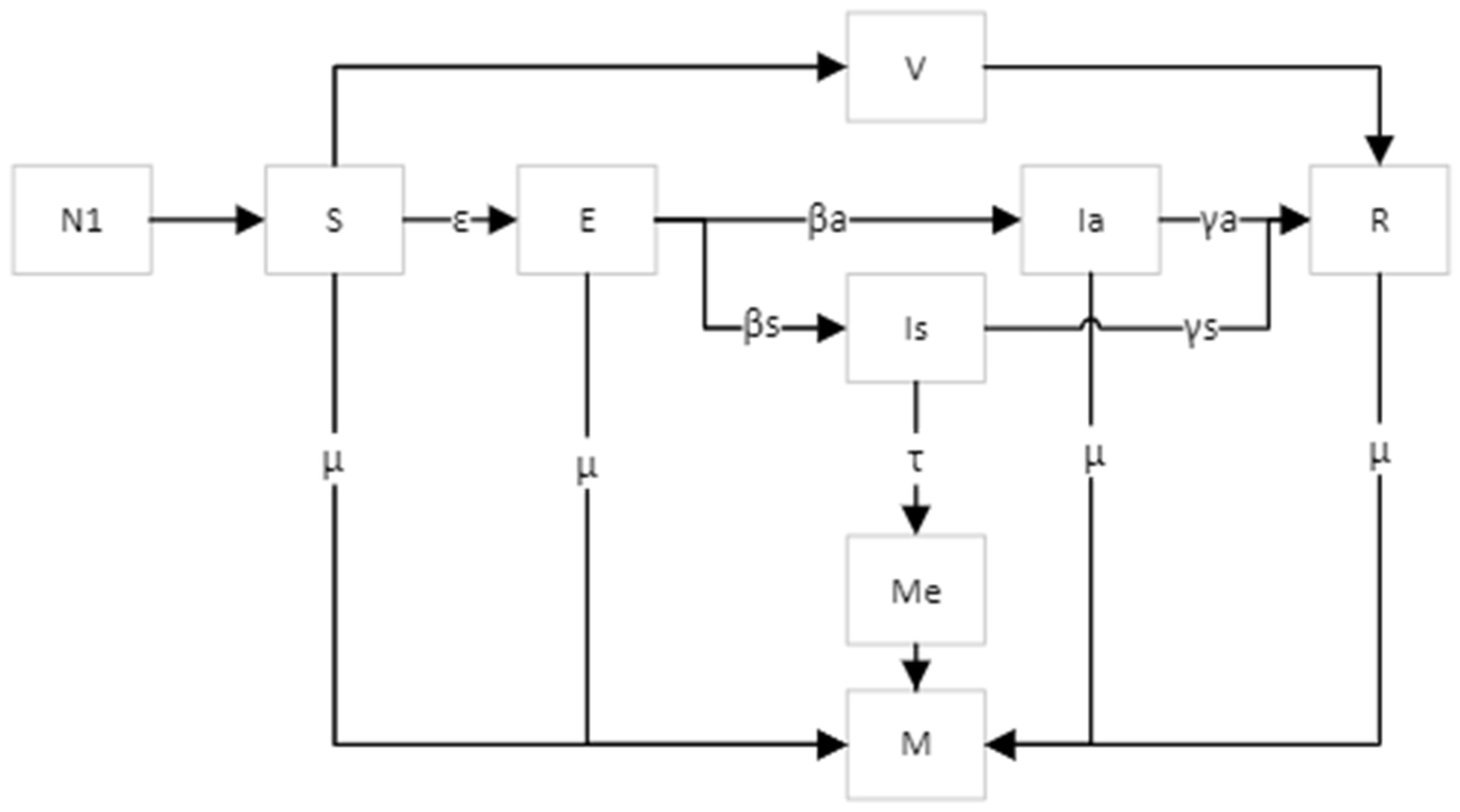
2.1. Model Development

First, the infection rates βs were calculated from a historical database covering the beginning of the pandemic. The initial conditions were determined via surveys to estimate the proportions of the population in various states: susceptible, in transition to infection, infected, recovered, and deceased from COVID-19. These initial conditions were arbitrarily adjusted according to the location of analysis, incorporating the subjective perception of the population in percentage form. This perception is considered critical, as it influences the infection rate through the biosecurity measures that people adopt. The model considers hand washing, the use of disinfectant alcohol, maintaining 2 m, and the use of protective glasses.
The model we developed was specifically designed to predict the spread of COVID-19 in Ecuador. We based our work on the SIR model, a standard in epidemiology that estimates the growth of infected people. The SIR model uses a system of differential equations in time, dividing the population into six distinct groups: susceptible S(t), in transition to infection N1(t) starting population exposed, E(t), infected I(t), recovered R(t), and deceased from COVID-19 Me(t) [28]. It was assumed that the total exposed population in a specific area remains constant, which was reflected in Equation (1) below. This equation was essential for understanding and modeling the evolution of the disease in each location during the pandemic period.
N 1 t = S o + I o + M e o + R o + E o
Regarding the model development, various other parameters were considered such as asymptomatic infections Ia(t), symptomatic infections Is(t), fatalities due to other causes M(t). Furthermore, an additional variable was introduced into the model: the daily vaccination rate, which can be arbitrarily integrated to examine disease spread. However, in this research, this variable has a value of zero and is only added when we want to consider a future scenario with a vaccination plan. The model also incorporated recovery rates for both symptomatic (γa) and asymptomatic (γs) populations. It was also accounted for the disease transmission factor (ε) and the COVID-19 mortality rate (τ). In this model, the inherent mortality rate of the population (μ) in the absence of the virus was addressed. These variables were utilized within the model to depict the dynamic changes in the system, as illustrated in Figure 1.
The population within the susceptible group comprised individuals at risk of acquiring the infection and transitioning to the infected population, whether presenting symptoms or not. From a mathematical perspective, the susceptible population group was modeled in relation to the total population, using the symptomatic infection factor βs. Simultaneously, another subset became infected without displaying symptoms, as characterized by the asymptomatic infection factor βa. The susceptible population underwent a state transition encompassing both the incubation period and the possibility of individuals succumbing to causes unrelated to COVID-19. Additionally, it was noted a segment of the susceptible population that had been vaccinated and was now immune to the virus, as depicted in Equation (2).
d s d t = β s S I s N 1 β a S I a N 1 μ S V
The transit stage refers to the period during which the infected group transitions from being susceptible to displaying symptoms, and it is represented as E(t), with a ɛ factor of 5.2 days [29]. Furthermore, when evaluating the model during this stage, consideration was given to the deceased population that was infected but died due to the overall population mortality unrelated to COVID-19, with a µ factor of 0.51% and 0.43% for Chile and Ecuador, respectively [6], as described in Equation (3).
d E d t = β s S I s N 1 + β a S I a N 1 ϵ E μ E
The infected population refers to individuals who have passed the transit stage and can either develop symptoms or remain asymptomatic. The α factor indicates that 30.8% of the infected population, after the transit stage, presents symptoms [30]. During this phase, the recovery or mortality of this group was associated with the recovery factor (γ) and the mortality factor (τ), which were estimated and projected based on the database. Equations (4)–(7) constitute a set of equations related to the infected population, both symptomatic and asymptomatic.
I a = I
I s = 1 I
d I s d t = 1 α ϵ E γ s I s τ I s μ I s
d I a d t = α ϵ E γ a I a μ I a
In the population that had surpassed the infection stage, whether asymptomatic or symptomatic, they were regarded as part of the recovery group. For this group, a γ factor of 14 days was employed as the necessary period to overcome the illness, which was uniformly applied to both asymptomatic (γa) and symptomatic (γs) individuals within the model’s context. Additionally, considerations were made for individuals who passed away due to causes unrelated to COVID-19. Those who had been vaccinated and experience milder effects of COVID-19 were also counted as part of the recovered population, as detailed in Equation (8).
d R d t = γ s I s + γ a I a μ R + V
The Ro factor, also known as the basic reproduction number, was a value that represents an infected person’s capacity to transmit the virus within their environment during the development of the disease. This factor was directly related to the COVID-19 infection rate and the recovery rate observed in the infected population. By analyzing this factor, we can assess the virus’s level of contagiousness and gain a deeper understanding of its effects on population dynamics, which was crucial for the model. Equation (9) presents the mathematical expression that quantifies this concept within the context of the analysis.
R o = β γ

2.2. Model Testing

The model was initially designed for application in the population of Ecuador. However, discrepancies were identified within its database, regarding the variability in the number of COVID-19 deaths during the months of April and May 2020, as reported by the Emergency Operations Council (COE) [4]. These data inconsistencies raised concerns about the reliability of the available information during the pandemic crisis. As a result, it was decided to choose reliable and consistent data that were found in Chile to test the model. The choice of the Chilean database was based on criteria of data frequency and availability, with the purpose of accurately and reliably assessing the behavior of COVID-19 within the model. Both countries share demographic similarities, but exhibit significantly different trends in COVID-19-related data, as illustrated in Figure 2.
For the model evaluation, first, an analysis was conducted on the population of Chile and subsequently on Ecuador. This analysis focused on the period from the initial records of confirmed cases to the commencement of the vaccination program, as this period exhibited similar conditions in both populations. In the case of Chile, the evaluation period spanned from 22 February to 23 December 2020, whereas for Ecuador, it extended from 29 February 2020 to 2 May 2021 [4,31]. To ensure uniform conditions, an arbitrary percentage value was implemented to reflect compliance with biosecurity measures in both populations, considering the probability of infection. These measures encompassed practices such as handwashing; the use of alcohol or hand sanitizer; maintaining 2-m social distancing; and the use of masks, gloves, and goggles.
Subsequently, the exposed population was divided into quartiles, and three tests were conducted for each of these quartiles. For the data related to the infected population, a dynamic variability of 1% was introduced every 14 days as a perturbation. This was carried out to assess the model’s robustness under the conditions that could introduce uncertainty into the data in Ecuador and to observe its evolution over time. It is important to note that while Chile was used to validate the model, the primary focus of this study was the population of Ecuador.
For the statistical analysis, a normality test of the residuals was applied by means of the Q-Q method for each projection, to determine the most appropriate test for evaluating the hypothesis. During the model validation process, Fisher’s Least Significant Difference (LSD) test with a confidence level of 95% was addressed. This methodology was utilized to compare the real data with the projections, allowing us to identify whether there was a significant difference between the model and the data published in Ecuador and Chile related to the spread of COVID-19.
One of the methods employed to validate the model was the Monte Carlo method, utilized to assess real data alongside predictions. This procedure was conducted for both Chile and Ecuador. The Mean Squared Error (MSE) was chosen as the statistical parameter to evaluate prediction accuracy, and a t-test was conducted to compare the means of MSE between both methods to determine if a significant difference existed. This approach facilitates a meticulous and statistically robust assessment of the prediction methods. Monte Carlo simulation, relying on random numbers to estimate numerical outcomes, becomes a valuable tool for evaluating method performance based on simulated data, thereby providing pertinent information for decision-making [32].

3. Results

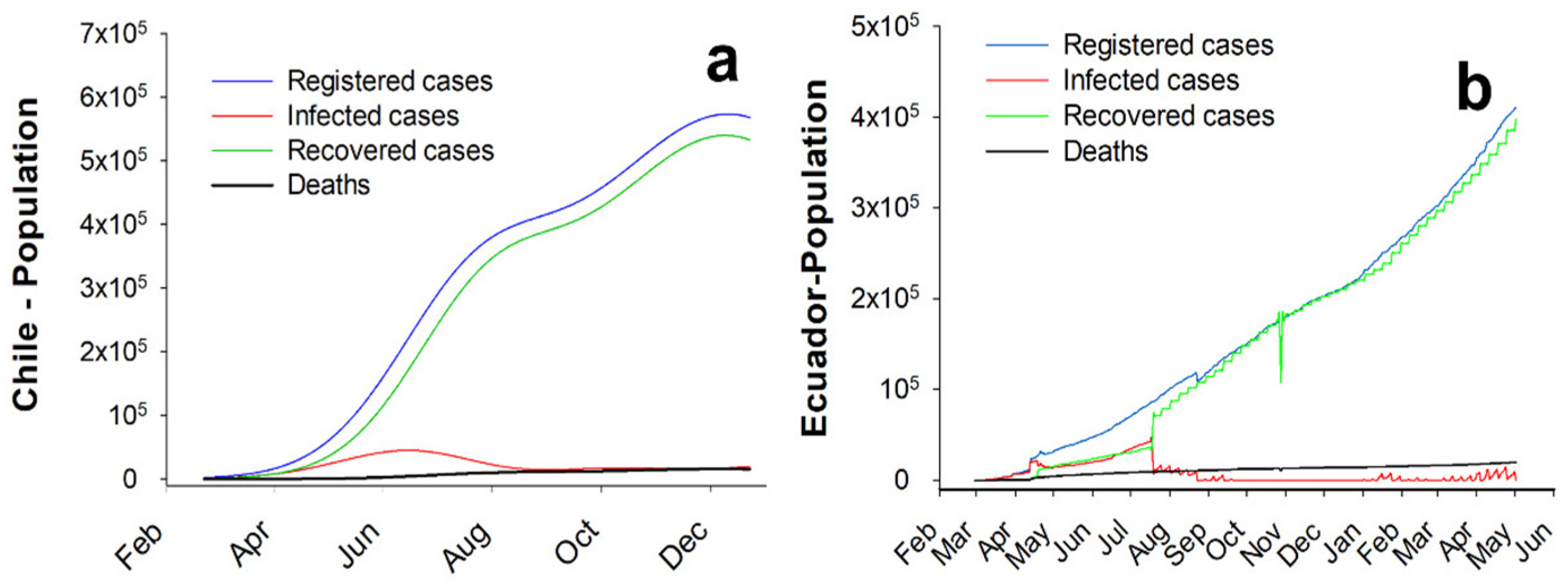
3.1. Database Model Testing

The behavior of Chile’s database regarding registered, infected, recovered, and deceased COVID-19 cases during the period from 22 February to 23 December 2020 is presented in Figure 2a. The curve exhibits noticeable data consistency, with an average Mean Absolute Error (MAE) of 8.47% for infected cases, in accordance with the model’s projections. Conversely, in Figure 2b, Ecuador’s database displays high variations on different dates that are contradictory and unrealistic in terms of variables such as registered cases, infections, recoveries, and COVID-19 deaths during the same period, prior to the implementation of the vaccination program.
The data were divided into quartiles with three tests for each projection when the disease symptoms started to appear on infected ones. There was normality in data calculated using the Q—Q Plot. The test for multiple ranks was applied to evaluate homogenous groups and determine if there is a relationship between forecast and real data. Indeed, Table 1 shows that forecast and real data homogeneity exists up to quartile 2 (Q2) according to a confidence level of 95%. Furthermore, when testing homogeneous group B using ANOVA analysis, the data indicate no significant statistical differences between real data and B homogeneous level due to a p-value of 0.902, with a level confidence of 95%.
The forecast error was analyzed based on the mean absolute error between real data and model forecast, showing errors within ranges from 6.33% (32,021.71 population) to 8.41% (33,639.93 population) for quartiles 2 and 3, respectively (Table 2).
The model analyses’ Pearson correlation factors between forecast and real data. The r values were 0.89 to Q1, 0.99 to Q2, and 1 to Q3 (Figure 3). Therefore, the model was validated by forecasting the period up to Q2 of analyzed data.

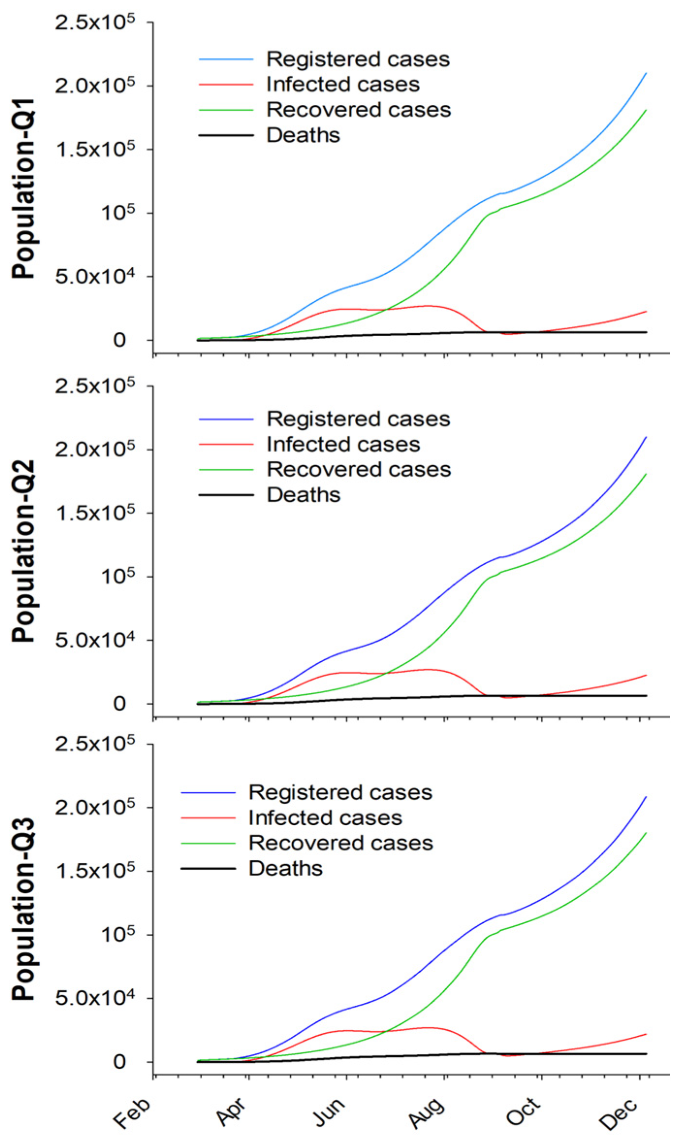
3.2. Ecuador Forecast Modelling

The model forecasted scenarios presenting the percentages of exposed individuals in groups of Q1, Q2, and Q3 and indicating similar values of infections without significant variation with an absolute mean error range of 3.83% to 4.38% for Q2 and Q3, respectively. This result shows that COVID-19 growth was independent of population exposure but dependent on the biosecurity measures requested in countries. Figure 3 illustrates the disease growth in three groups with similar trends.
On 23 December 2020, 13,612 people died of circumstances and symptoms related to COVID-19 [33]. Furthermore, a countless number of the infected population in the database died as of May of 2021, fluctuating to 42,000 (Figure 2). This situation caused inefficient management and decision making based on nonexistent data, turning the pandemic before the vaccination into a very difficult period to manage. In the beginning, when infected people started to test positive, the curve rapidly grew exponentially to the extent that it was impossible to trace the infection hot spots. Then, the mathematical model forecasted the growth of infected people since the spread of COVID-19, which was directly related to biosecurity measures adopted by the population. Therefore, these variables were determined when the infectious probability was based on their biosecurity. The dynamic models considered epidemiological parameters such as infection and recovery rates of sampled people and using these factors, which were dynamically predicted, smoothing the database curves of Ecuador.
In the case of Ecuador, the model considers biosecurity measures and the exposed population to the virus as the initial state. Then, it calculates the epidemic factors from the database, and finally, the dynamic model projects and analyses possible scenarios of infected, recovered, and deceased populations from the beginning to the end of the infection, as Table 3 reflects. The results showed that the Ro of infected and deceased populations are strictly related to the population exposed. Therefore, the infection numbers exponentially grew due to the people exposed. Furthermore, if the model varies these conditions, the results might indicate different values depending on people’s behavior.
Indeed, applying mathematical models to predict the potential impact, transmission growth rate, and virus identification was essential to mitigate the effects of this epidemic [9,34,35]. Worldwide, the use of Machine Learning and Deep Learning gives relevant information to assist medical and governmental agencies in advance [36,37,38,39].
Another method used to assess the projections involved applying the Monte Carlo method to compare real data from Chile and Ecuador. The results displayed a Mean Squared Error of 0.15% for Chile and 0.31% for Ecuador, both below 10%, showcasing the accuracy of the projections in relation to actual data. Subsequently, an evaluation of each Mean Squared Error was carried out through a t-test, indicating that there was no significant difference between the real data and the projections with a 95% confidence level. This analysis covered the period from 22 February to 23 December 2020, and a total of 1000 simulations were conducted following [40] methodology. These results substantiate the model’s robustness and effectiveness in the decision making process.

4. Discussion

Reported cases of SARS-CoV-2 or COVID-19 continue to increase worldwide due to person-to-person transmission of coronavirus diseases. As of 13 September 2023, according to [1], a total of 770,563,467 confirmed cases of COVID-19 have reported, resulting in 6,957,216 deaths. Thus, the prediction was the highest priority for controlling and managing resource-limited diseases [10]. This model predicted the spread of COVID-19 or SARS-CoV-2 virus based on infection, transit, and recovery factors that allow the calculation of a basic reproduction number (Ro). This study proposed and simulated COVID-19 transmission dynamics based on accessible data [4] for Ecuador from 29 February 2020 to 2 May 2021. However, the availability of data in Ecuador was a limiting factor for the model validation, so the data from Chile were collected from 22 February to 23 December 2020. Mathematical models are essential in decision making during outbreak control [41,42]. To determine pandemic expansion, It is necessary to estimate the Ro of the infectious disease, which must be reduced to an Ro of 1 or less to eliminate the outbreak. For example, a Ro = 2.5 represents a fraction of 60.0% [13]. In this model, the Ro was established based on population exposure, which was divided into quartiles of 25%, 50%, and 75% of the exposed population. The average estimated Ro was 3.42 (95% CI, 3.62 and 3.22). This value was higher than the global mean established by the WHO between 1.4 to 2.5 [43,44], but it was closer to the global Ro of 3.32 (95% CI, 2.81 to 3.82) determined by [13], which in the worldwide meta-analysis, established that these Ro ranges were closer to the reality, because they verified that the virus presented at least more than one generation of transmission. The estimated Ro confirmed that the reproduction and expansion of the virus were greater in Ecuador than in other countries in different periods of the year 2020. The Ro for India was 1.66 [10], Ro for Africa was 2.37 [45], and for several states of the United States, was 1.66 (IQR: 1.35–2.11) [46]. However, in this study, the R0 was smaller than the one determined for Brazil between 26 February 2020 and 25 March 2020, which was 5.25 [47]. In contrast, for this research, the Ro value was like the one found by [48], which resulted in the Ro in Ecuador reaching a maximum exponential growth of 3.45. In other words, the result presented in this investigation would explain a high wave of infection in the country. Therefore, the Ro was higher than the one found by [49], who established a value of 2.2 with 88% of susceptible/infected individuals. The Ro estimates for COVID-19, including the study Ro, were higher than the Ro values estimated for epidemics caused by coronaviruses that had high dissemination at the beginning of the century and the previous decade, such as the cases of Severe Acute Respiratory Syndrome (SARS) spread in Beijing, China, at the end of 2002 that affected at least 37 countries, with an estimated R0 between 2.2 to 4.91, and the Middle East Respiratory Syndrome (MERS) of 2012 had an R0 between 0.29 and 0.80 in 27 countries [44,50,51,52]. These data suggest that the spread and expansion of COVID-19 has been greater than other coronaviruses. Furthermore, the dynamic model that was created to test Ecuador differs from other models applied. For example, in India’s population of 1 billion, the virus dispersion was exponential, without considering biosecurity measures and only focusing on infected people [8]. Ref. [9] analyzed the disease growth based on confidence bounds by using the growing trend of COVID-19 in countries such as Switzerland, the United Kingdom, the Netherlands, Austria, Belgium, Norway, and Sweden, showing that the virus growth was exponential. This type of projection did not consider the factors that influenced the disease increase, which were intrinsic to the population and dynamic in time, limiting only to deterministic projections. The estimated Ro depends on factors such as the biology of the infectious agent, the simulation method used, the validity of the hypotheses considered, and fundamentally, the integration of social, demographic, or environmental variables that adequately characterize the environment [13,53]. The frequency of contact might depend on population size and social, economic, or cultural factors, which might vary from one locality to another [54]. In addition, the Ro estimates might be somewhat prone to error due to factors such as a short period of analysis, insufficient data, or both [55]. While the Ro values typically occur high in the early stages of an epidemic, both because of small sample size and lack of disease awareness, this does not mean that Ro values do not vary between different populations and even between subgroups within the same population [17,56]. One factor that might directly impact this variation is social behavior at the onset of the pandemic, characterized by failure to take adequate preventive measures [57,58]. Given the rapid spread of the disease and the high dependence of its control on the effectiveness of policies or guidelines that regulate or control social behavior, COVID-19 appeared to be relatively difficult to control [59]. The results suggested that prevention and containment measures such as confinement and social distancing were more than necessary to control this pandemic [60,61]. These actions, along with access to medical facilities and rapid population testing, significantly impacted the spread and thus, the cases and casualties [37,62]. All these aspects will undoubtedly influence traditional simulation methods and processes, while learning algorithms could be adapted, especially if multiple datasets are available for a given region. This approach can not only outperform SIR models but requires fewer input data to estimate trends and has a computational cost of about 0.24 s. Although, reliable results for Ecuadorian data were depicted, the lack and inconsistency led us to investigate the more consistent and regular data from a neighboring country, Chile, to validating estimates. This situation was necessary in order to continue testing these approaches and methods by means of other databases worldwide. Nevertheless, the results presented here emerged as a valuable and valid source of information and tool for evidence-based decision making.

5. Conclusions

The present study attempted to predict the spread in Ecuador using a basic reproduction number (Ro) in a dynamic model simulation. The main finding is that the estimated Ro for COVID-19 in Ecuador was 3.42, higher than the global average for COVID-19 in 2020, and even higher than previous epidemics of other coronaviruses such as SARS and MERS. The research findings confirmed that Ecuador was one of the countries where the virus spread the fastest. It is essential to emphasize that multiple factors, including social behaviors and preventive measures, influence the Ro value. Although, the development of a multivariate dynamic COVID-19 model based on the SIR model was able to predict the spread of the virus in the population of Ecuador. The validation of the model was performed by using data of the infection and spread of the virus from Chile, due to the lack of data of Ecuador.
The results showed that the mean absolute error is 4.21% and thus, the forecast based on data from Ecuador depicted the percentages of population exposure, without considering biosecurity measures for the spread of COVID-19. Therefore, the model could forecast up to Q2 of the database over time, with an error of no more than 10%. The forward simulation could predict variations within a linear system of the biosecurity measures taken by the population when exposed to the virus.
One of the main limitations of this model was the lack and inconsistency of the data, which led us to resort using more consistent and regular data from a neighboring country, such as Chile, to validate it. This situation was necessary in order to continue testing these approaches and methods in other databases worldwide. Additionally, it was noted that the accuracy of this model could be affected by changes in the virus’s transmission dynamics, such as the emergence of new variants or changes in social distancing measures. Therefore, the model’s performance must be continuously evaluated and updated as new data become available. Finally, it is recommended that for future research endeavors, enhancing the model’s accuracy should be pursued through the incorporation of supplementary variables, such as demographic and environmental factors, alongside the utilization of more advanced machine learning techniques.
This study delves into the impact of multiple factors on traditional simulation methods, with a particular emphasis on the adaptability of learning algorithms, especially when multiple datasets are accessible for a specific region. The proposed approach not only surpasses traditional SIR models but also operates efficiently, requiring fewer input data and boasting a low computational cost (approximately 0.24 s). However, it is important to note that while the study provides reliable results for Ecuadorian data, the limitations due to data scarcity and inconsistency led to the use of more consistent Chilean data for validation. This highlights the necessity of further testing and refinement of these methods in diverse global datasets. Nevertheless, these findings are a valuable resource for evidence-based decision making, particularly in the realm of public health and COVID-19 management and control, offering practical implications for resource allocation, vaccination campaigns, and social distancing measures.

Author Contributions

Conceptualization, J.G.; methodology, J.G.; software, J.G.; validation, J.G., J.C.G., K.P., P.A.-M., G.J., S.C., L.Á., H.C. and B.B.; formal analysis, J.G., J.C.G. and K.P.; investigation, J.C.G., K.P., P.A.-M., G.J., S.C. and L.Á.; resources, J.C.G., K.P., P.A.-M., G.J., S.C. and L.Á.; data curation, J.G.; writing—original draft preparation, J.G., P.A.-M., J.C.G. and K.P.; writing—review and editing, P.A.-M., G.J. and S.C.; visualization, J.G. and J.C.G.; supervision, resources, funding acquisition, J.G. and J.C.G. All authors have read and agreed to the published version of the manuscript.

Funding

The authors thank Universidad Técnica del Norte for supporting this research.

Data Availability Statement

COVID-19 Statistics, the government of Ecuador. https://www.coronavirusecuador.com/estadisticas-COVID-19/ (accessed on 14 January 2022). Data: National situation of COVID-19 in Chile, government of Chile. https://www.gob.cl/pasoapaso/cifrasoficiales/#datos (accessed on 21 October 2021).

Acknowledgments

Universidad Técnica del Norte was the institution that contributed to funding this study by providing all the technological tools to achieve the objectives.

Conflicts of Interest

The authors declare no conflict of interest.

References

  1. WHO (World Health Organization). WHO Coronavirus (COVID-19) Dashboard. 2023. Available online: https://covid19.who.int/ (accessed on 5 September 2023).
  2. Spychalski, P.; Błażyńska-Spychalska, A.; Kobiela, J. Estimating Case Fatality Rates of COVID-19. Lancet Infect. Dis. 2020, 20, 774–775. [Google Scholar] [CrossRef] [PubMed]
  3. Verity, R.; Okell, L.C.; Dorigatti, I.; Winskill, P.; Whittaker, C.; Imai, N.; Cuomo-Dannenburg, G.; Thompson, H.; Walker, P.G.; Fu, H.; et al. Estimates of the Severity of COVID-19 Disease. MedRxiv 2020, 2020-03. [Google Scholar]
  4. Gobierno de la República de Ecuador. Estadísticas COVID-19—Coronavirus Ecuador. 2022. Available online: https://www.coronavirusecuador.com/estadisticas-covid-19/ (accessed on 14 January 2022).
  5. Duque-Rengel, V.K.; Márquez-Domínguez, C.; Calva-Cabrera, K.D.; Zambrano, C.M.B. Comunicación Gubernamental y Redes Sociales Durante La Pandemia de 2020 En Ecuador: Derechos Humanos y Mensajes Educativos. Rev. Ibérica Sist. Tecnol. Informação 2021, 180–198. [Google Scholar]
  6. Vera, F.; Solórzano, M.; Ochoa, G.; García Bustos, S.; Cevallos, S. Mortality Tables of Continental Ecuador Using a Survival Analysis. Papeles De Población 2018, 24, 63–83. [Google Scholar] [CrossRef]
  7. Fanelli, D.; Piazza, F. Analysis and Forecast of COVID-19 Spreading in China, Italy and France. Chaos Solitons Fractals 2020, 134, 109761. [Google Scholar] [CrossRef] [PubMed]
  8. Khajanchi, S.; Sarkar, K.; Mondal, J. Dynamics of the COVID-19 Pandemic in India. arXiv 2020, arXiv:2005.06286. [Google Scholar] [CrossRef]
  9. Kumar, P.; Kalita, H.; Patairiya, S.; Sharma, Y.D.; Nanda, C.; Rani, M.; Rahmani, J.; Bhagavathula, A.S. Forecasting the Dynamics of COVID-19 Pandemic in Top 15 Countries in April 2020: ARIMA Model with Machine Learning Approach. MedRxiv 2020, 2020-03. [Google Scholar] [CrossRef]
  10. Samui, P.; Mondal, J.; Khajanchi, S. A Mathematical Model for COVID-19 Transmission Dynamics with a Case Study of India. Chaos Solitons Fractals 2020, 140, 110173. [Google Scholar] [CrossRef]
  11. Vespignani, A.; Tian, H.; Dye, C.; Lloyd-Smith, J.O.; Eggo, R.M.; Shrestha, M.; Scarpino, S.V.; Gutierrez, B.; Kraemer, M.U.; Wu, J.; et al. Modelling COVID-19. Nat. Rev. Phys. 2020, 2, 279–281. [Google Scholar] [CrossRef]
  12. Restif, O.; Hayman, D.T.; Pulliam, J.R.; Plowright, R.K.; George, D.B.; Luis, A.D.; Cunningham, A.A.; Bowen, R.A.; Fooks, A.R.; O’Shea, T.J.; et al. Model-Guided Fieldwork: Practical Guidelines for Multidisciplinary Research on Wildlife Ecological and Epidemiological Dynamics. Ecol. Lett. 2012, 15, 1083–1094. [Google Scholar] [CrossRef]
  13. Alimohamadi, Y.; Taghdir, M.; Sepandi, M. Estimate of the Basic Reproduction Number for COVID-19: A Systematic Review and Meta-Analysis. J. Prev. Med. Public Health 2020, 53, 151–157. [Google Scholar] [CrossRef] [PubMed]
  14. Kermack, W.O.; McKendrick, A.G. Contributions to the Mathematical Theory of Epidemics–I. 1927. Bull. Math. Biol. 1991, 53, 33–55. [Google Scholar] [PubMed]
  15. Shaw, C.L.; Kennedy, D.A. What the Reproductive Number R 0 Can and Cannot Tell Us about COVID-19 Dynamics. Theor. Popul. Biol. 2021, 137, 2–9. [Google Scholar] [CrossRef] [PubMed]
  16. Yuan, J.; Li, M.; Lv, G.; Lu, Z.K. Monitoring Transmissibility and Mortality of COVID-19 in Europe. Int. J. Infect. Dis. 2020, 95, 311–315. [Google Scholar] [CrossRef] [PubMed]
  17. Delamater, P.L.; Street, E.J.; Leslie, T.F.; Yang, Y.T.; Jacobsen, K.H. Complexity of the Basic Reproduction Number (R0). Emerg. Infect. Dis. 2019, 25, 1. [Google Scholar] [CrossRef] [PubMed]
  18. Omori, R.; Mizumoto, K.; Chowell, G. Changes in Testing Rates Could Mask the Novel Coronavirus Disease (COVID-19) Growth Rate. Int. J. Infect. Dis. 2020, 94, 116–118. [Google Scholar] [CrossRef] [PubMed]
  19. Hethcote, H.W. The basic epidemiology models: Models, expressions for R0, parameter estimation, and applications. In Mathematical Understanding of Infectious Disease Dynamics; Lecture Notes Series, Institute for Mathematical Sciences, National University of Singapore; World Scientific: Singapore, 2008; Volume 16, pp. 1–61. ISBN 978-981-283-482-9. [Google Scholar]
  20. Zhao, J.; Wang, Z.; Dong, Y.; Yang, Z.; Govers, G. How Soil Erosion and Runoff Are Related to Land Use, Topography and Annual Precipitation: Insights from a Meta-Analysis of Erosion Plots in China. Sci. Total Environ. 2022, 802, 149665. [Google Scholar] [CrossRef] [PubMed]
  21. Zhang, H.; Wei, J.; Yang, Q.; Baartman, J.E.M.; Gai, L.; Yang, X.; Li, S.; Yu, J.; Ritsema, C.J.; Geissen, V. An Improved Method for Calculating Slope Length (λ) and the LS Parameters of the Revised Universal Soil Loss Equation for Large Watersheds. Geoderma 2017, 308, 36–45. [Google Scholar] [CrossRef]
  22. Ferrari, M.J.; Bjørnstad, O.N.; Dobson, A.P. Estimation and Inference of R0 of an Infectious Pathogen by a Removal Method. Math. Biosci. 2005, 198, 14–26. [Google Scholar] [CrossRef]
  23. Anderson, R.M.; Heesterbeek, H.; Klinkenberg, D.; Hollingsworth, T.D. How Will Country-Based Mitigation Measures Influence the Course of the COVID-19 Epidemic? Lancet 2020, 395, 931–934. [Google Scholar] [CrossRef]
  24. Bates, I.; Fenton, C.; Gruber, J.; Lalloo, D.; Lara, A.M.; Squire, S.B.; Theobald, S.; Thomson, R.; Tolhurst, R. Vulnerability to Malaria, Tuberculosis, and HIV/AIDS Infection and Disease. Part 1: Determinants Operating at Individual and Household Level. Lancet Infect. Dis. 2004, 4, 267–277. [Google Scholar] [CrossRef] [PubMed]
  25. Khalatbari-Soltani, S.; Cumming, R.G.; Delpierre, C.; Kelly-Irving, M. Importance of Collecting Data on Socioeconomic Determinants from the Early Stage of the COVID-19 Outbreak Onwards. J. Epidemiol. Community Health 2020, 74, 620–623. [Google Scholar] [CrossRef] [PubMed]
  26. Liang, J.; Zhang, X.; Wang, K.; Tang, M.; Tian, M. Discovering Dynamic Models of COVID-19 Transmission. Transbounding Emerg. Dis. 2022, 69, e64–e70. [Google Scholar] [CrossRef] [PubMed]
  27. Wang, M.; Flessa, S. Modelling COVID-19 under Uncertainty: What Can We Expect? Eur. J. Health Econ. 2020, 21, 665–668. [Google Scholar] [CrossRef] [PubMed]
  28. Rachah, A.; Torres, D.F. Mathematical Modelling, Simulation, and Optimal Control of the 2014 Ebola Outbreak in West Africa. Discret. Dyn. Nat. Soc. 2015, 2015, 842792. [Google Scholar] [CrossRef]
  29. Hamzah, F.B.; Lau, C.; Nazri, H.; Ligot, D.V.; Lee, G.; Tan, C.L.; Shaib, M.; Zaidon, U.H.B.; Abdullah, A.B.; Chung, M.H.; et al. CoronaTracker: Worldwide COVID-19 Outbreak Data Analysis and Prediction. Bull. World Health Organ. 2020, 1, 1–32. [Google Scholar] [CrossRef]
  30. BBC News Mundo. Coronavirus: ¿cuándo Una Persona Enferma de COVID-19 Deja de Ser Contagiosa (Tenga o No Síntomas)? 2021. Available online: https://www.bbc.com/mundo/noticias-55988371 (accessed on 21 October 2021).
  31. Gobierno de Chile. Cifras: Situación Nacional Del COVID-19 En Chile 2020. Available online: https://www.gob.cl/pasoapaso/cifrasoficiales/#datos (accessed on 21 October 2021).
  32. Robert, C.P.; Casella, G. Monte Carlo Statistical Methods, 2nd ed.; Springer: New York, NY, USA, 2004; Volume 2. [Google Scholar]
  33. El Universo Casos de Coronavirus En Ecuador, al Jueves 3 de Diciembre: 195.884 Confirmados y 13.612 Fallecidos 2020. Available online: https://www.eluniverso.com/noticias/2020/12/03/nota/8070727/coronavirus-covid19-ecuador-casos-contagios-muertes-3-diciembre/ (accessed on 21 October 2021).
  34. Harjule, P.; Tiwari, V.; Kumar, A. Mathematical Models to Predict COVID-19 Outbreak: An Interim Review. J. Interdiscip. Math. 2021, 24, 259–284. [Google Scholar] [CrossRef]
  35. Muniyappan, A.; Sundarappan, B.; Manoharan, P.; Hamdi, M.; Raahemifar, K.; Bourouis, S.; Varadarajan, V. Stability and Numerical Solutions of Second Wave Mathematical Modeling on COVID-19 and Omicron Outbreak Strategy of Pandemic: Analytical and Error Analysis of Approximate Series Solutions by Using HPM. Mathematics 2022, 10, 343. [Google Scholar] [CrossRef]
  36. Ní Fhloinn, E.; Fitzmaurice, O. Challenges and Opportunities: Experiences of Mathematics Lecturers Engaged in Emergency Remote Teaching during the COVID-19 Pandemic. Mathematics 2021, 9, 2303. [Google Scholar] [CrossRef]
  37. Pinter, G.; Felde, I.; Mosavi, A.; Ghamisi, P.; Gloaguen, R. COVID-19 Pandemic Prediction for Hungary; A Hybrid Machine Learning Approach. Mathematics 2020, 8, 890. [Google Scholar] [CrossRef]
  38. Saleem, F.; AL-Ghamdi, A.S.A.-M.; Alassafi, M.O.; AlGhamdi, S.A. Machine Learning, Deep Learning, and Mathematical Models to Analyze Forecasting and Epidemiology of COVID-19: A Systematic Literature Review. Int. J. Environ. Res. Public Health 2022, 19, 5099. [Google Scholar] [CrossRef] [PubMed]
  39. Vytla, V.; Ramakuri, S.K.; Peddi, A.; Srinivas, K.K.; Ragav, N.N. Mathematical Models for Predicting COVID-19 Pandemic: A Review. J. Phys. Conf. Ser. 2021, 1797, 012009. [Google Scholar] [CrossRef]
  40. Xie, G. A Novel Monte Carlo Simulation Procedure for Modelling COVID-19 Spread over Time. Sci. Rep. 2020, 10, 13120. [Google Scholar] [CrossRef] [PubMed]
  41. Egger, M.; Johnson, L.; Althaus, C.; Schöni, A.; Salanti, G.; Low, N.; Norris, S.L. Developing WHO Guidelines: Time to Formally Include Evidence from Mathematical Modelling Studies. F1000Research 2017, 6, 1584. [Google Scholar] [CrossRef] [PubMed]
  42. James, L.P.; Salomon, J.A.; Buckee, C.O.; Menzies, N.A. The Use and Misuse of Mathematical Modeling for Infectious Disease Policymaking: Lessons for the COVID-19 Pandemic. Med. Decis. Mak. 2021, 41, 379–385. [Google Scholar] [CrossRef] [PubMed]
  43. Liu, S.L.; Dong, Y.H.; Li, D.; Liu, Q.; Wang, J.; Zhang, X.L. Effects of Different Terrace Protection Measures in a Sloping Land Consolidation Project Targeting Soil Erosion at the Slope Scale. Ecol. Eng. 2013, 53, 46–53. [Google Scholar] [CrossRef]
  44. Wu, J.T.; Leung, K.; Leung, G.M. Nowcasting and Forecasting the Potential Domestic and International Spread of the 2019-nCoV Outbreak Originating in Wuhan, China: A Modelling Study. Lancet 2020, 395, 689–697. [Google Scholar] [CrossRef]
  45. Musa, S.S.; Zhao, S.; Wang, M.H.; Habib, A.G.; Mustapha, U.T.; He, D. Estimation of Exponential Growth Rate and Basic Reproduction Number of the Coronavirus Disease 2019 (COVID-19) in Africa. Infect. Dis. Poverty 2020, 9, 96. [Google Scholar] [CrossRef]
  46. Sy, K.T.L.; White, L.F.; Nichols, B.E. Population Density and Basic Reproductive Number of COVID-19 across United States Counties. PLoS ONE 2021, 16, e0249271. [Google Scholar] [CrossRef]
  47. Crokidakis, N. Modeling the Early Evolution of the COVID-19 in Brazil: Results from a Susceptible–Infectious–Quarantined–Recovered (SIQR) Model. Int. J. Mod. Phys. C 2020, 31, 2050135. [Google Scholar] [CrossRef]
  48. Fernández-Naranjo, R.P.; Vásconez-González, E.; Simbaña-Rivera, K.; Gómez-Barreno, L.; Izquierdo-Condoy, J.S.; Cevallos-Robalino, D.; Ortiz-Prado, E. Statistical Data Driven Approach of COVID-19 in Ecuador: R 0 and R t Estimation via New Method. Infect. Dis. Model. 2021, 6, 232–243. [Google Scholar] [CrossRef] [PubMed]
  49. Espinosa, P.; Quirola-Amores, P.; Teran, E. Application of a Susceptible, Infectious, and/or Recovered (SIR) Model to the COVID-19 Pandemic in Ecuador. Front. Appl. Math. Stat. 2020, 6, 571544. [Google Scholar] [CrossRef]
  50. Breban, R.; Riou, J.; Fontanet, A. Interhuman Transmissibility of Middle East Respiratory Syndrome Coronavirus: Estimation of Pandemic Risk. Lancet 2013, 382, 694–699. [Google Scholar] [CrossRef] [PubMed]
  51. Gumel, A.B.; Ruan, S.; Day, T.; Watmough, J.; Brauer, F.; Van den Driessche, P.; Gabrielson, D.; Bowman, C.; Alexander, M.E.; Ardal, S.; et al. Modelling Strategies for Controlling SARS Outbreaks. Proc. R. Soc. Lond. Ser. B Biol. Sci. 2004, 271, 2223–2232. [Google Scholar] [CrossRef] [PubMed]
  52. Liu, Y.; Gayle, A.A.; Wilder-Smith, A.; Rocklöv, J. The Reproductive Number of COVID-19 Is Higher Compared to SARS Coronavirus. J. Travel Med. 2020, 27, taaa021. [Google Scholar] [CrossRef] [PubMed]
  53. Bustamante-Orellana, C.; Cevallos-Chavez, J.; Montalvo-Clavijo, C.; Sullivan, J.; Michael, E.; Mubayi, A. Modeling and Preparedness: The Transmission Dynamics of COVID-19 Outbreak in Provinces of Ecuador. MedRxiv 2020. [Google Scholar] [CrossRef]
  54. Vigl, J.; Strauss, H.; Talamini, F.; Zentner, M. Relationship Satisfaction in the Early Stages of the COVID-19 Pandemic: A Cross-National Examination of Situational, Dispositional, and Relationship Factors. PLoS ONE 2022, 17, e0264511. [Google Scholar] [CrossRef] [PubMed]
  55. Blumberg, S.; Lloyd-Smith, J.O. Comparing Methods for Estimating R0 from the Size Distribution of Subcritical Transmission Chains. Epidemics 2013, 5, 131–145. [Google Scholar] [CrossRef]
  56. Pandit, J. Managing the R0 of COVID-19: Mathematics Fights Back. Anaesthesia 2020, 75, 1643. [Google Scholar] [CrossRef]
  57. Oraby, T.; Tyshenko, M.G.; Maldonado, J.C.; Vatcheva, K.; Elsaadany, S.; Alali, W.Q.; Longenecker, J.C.; Al-Zoughool, M. Modeling the Effect of Lockdown Timing as a COVID-19 Control Measure in Countries with Differing Social Contacts. Sci. Rep. 2021, 11, 3354. [Google Scholar] [CrossRef]
  58. Shafer, L.A.; Nesca, M.; Balshaw, R. Relaxation of Social Distancing Restrictions: Model Estimated Impact on COVID-19 Epidemic in Manitoba, Canada. PLoS ONE 2021, 16, e0244537. [Google Scholar] [CrossRef]
  59. He, D.; Zhao, S.; Xu, X.; Lin, Q.; Zhuang, Z.; Cao, P.; Wang, M.H.; Lou, Y.; Xiao, L.; Wu, Y.; et al. Low Dispersion in the Infectiousness of COVID-19 Cases Implies Difficulty in Control. BMC Public Health 2020, 20, 1558. [Google Scholar] [CrossRef]
  60. Henry, B.F. Social Distancing and Incarceration: Policy and Management Strategies to Reduce COVID-19 Transmission and Promote Health Equity through Decarceration. Health Educ. Behav. 2020, 47, 536–539. [Google Scholar] [CrossRef]
  61. Sun, C.; Zhai, Z. The Efficacy of Social Distance and Ventilation Effectiveness in Preventing COVID-19 Transmission. Sustain. Cities Soc. 2020, 62, 102390. [Google Scholar] [CrossRef]
  62. Łukasik, M.; Porębska, A. Responsiveness and Adaptability of Healthcare Facilities in Emergency Scenarios: COVID-19 Experience. Int. J. Environ. Res. Public Health 2022, 19, 675. [Google Scholar] [CrossRef] [PubMed]
Figure 1. Unifilar diagram of COVID-19 Model.
Mathematics 11 04721 g001
Figure 2. COVID-19 growth curve of cases. (a) COVID-19 growth curve of cases in Chile from 22 February to 23 December 2020, (b) COVID-19 growth curve of cases in Ecuador from 29 February 2020 to 2 May 2021.
Mathematics 11 04721 g002
Figure 3. Disease growth forecast of 3 groups Q1, Q2, and Q3 quartiles.
Mathematics 11 04721 g003
Table 1. Test of Multiple Ranks.
TestCasesMeanHomogenous Groups
Chile 25% (Q1)-3306170,128A
Chile 25% (Q1)-2306171,818A
Chile 25%(Q1)-1306175,680A
Chile 50% (Q2)-2306279,780B
Chile 50%(Q2)-3306281,193B
Chile 50%(Q2)-1306281,381B
Chile 75%(Q3)-2306290,504B
Chile 75%(Q3)-3306290,632B
Chile 75% (Q3)-1306290,687B
Chile Real Data306298,163B
Table 2. Chile’s Mean Absolute Error Analysis.
Forecast Q1
1
Q1
2
Q1
3
Q2
1
Q2
2
Q2
3
Q3
1
Q3
2
Q3
3
Mean Absolute Error (%)47.4748.3848.858.478.628.416.336.396.34
Mean Forecast Error (population × 1000)163.61168.77171.0333.25 36.5033.6432.0232.7632.24
Table 3. Possible projected scenarios related to biosecurity measures of the infected, recovered, and deceased population of COVID-19 in Ecuador.
Biosecurity Measures *
[%]
Exposed
Population
RoConfirmed Cases
[Million]
DeathsInfected
Population
[%]
Wash hands9025%3.42274.0454,31223.21
Antiseptic gel90
Social distance (2 m)51
Face mask80
Globes1050%3.61738.04101,13146.25
Face shield1075%3.220412.05142,28569.28
* These percentages were random; however, small samples of people were taken in Imbabura to set the values.
Disclaimer/Publisher’s Note: The statements, opinions and data contained in all publications are solely those of the individual author(s) and contributor(s) and not of MDPI and/or the editor(s). MDPI and/or the editor(s) disclaim responsibility for any injury to people or property resulting from any ideas, methods, instructions or products referred to in the content.

