
Silver Price Forecasting Using Extreme Gradient Boosting (XGBoost) Method


Abstract
:1. Introduction
2. Materials and Methods
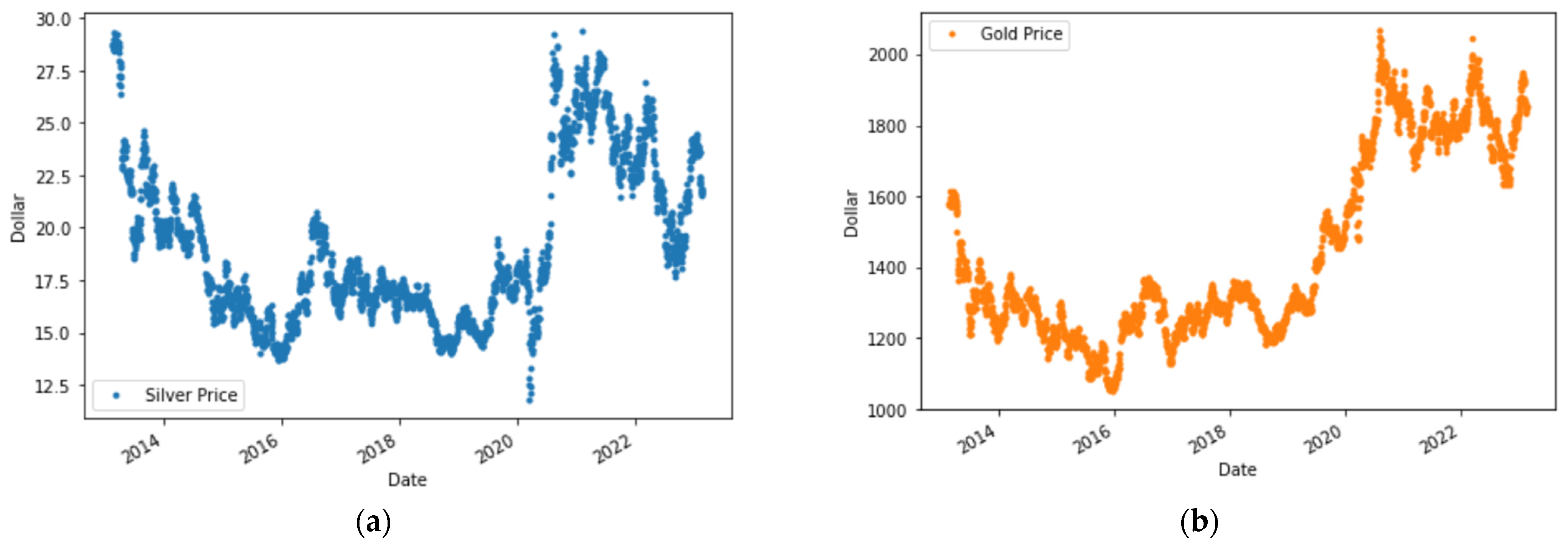
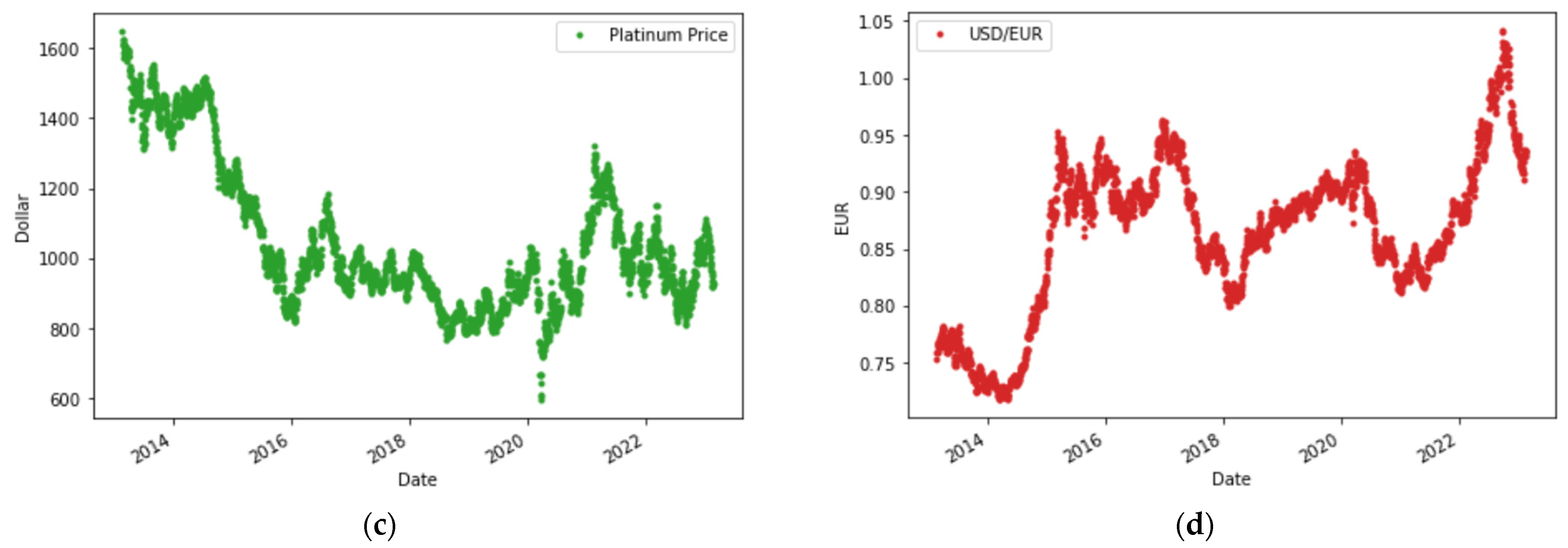
2.1. Data Collection
2.2. Random Forest
2.3. CatBoost
2.4. Extreme Gradient Boosting
2.5. Hyperparameter Tuning
2.6. Model Evaluation
2.6.1. Mean Absolute Percentage Error
2.6.2. Root Mean Square Error
2.6.3. Mean Absolute Error
2.6.4. Scatter Index
2.6.5. K-Fold Cross Validation
3. Methodology
4. Results and Discussion
4.1. Initial Model
4.2. Hyperparameter Tuning
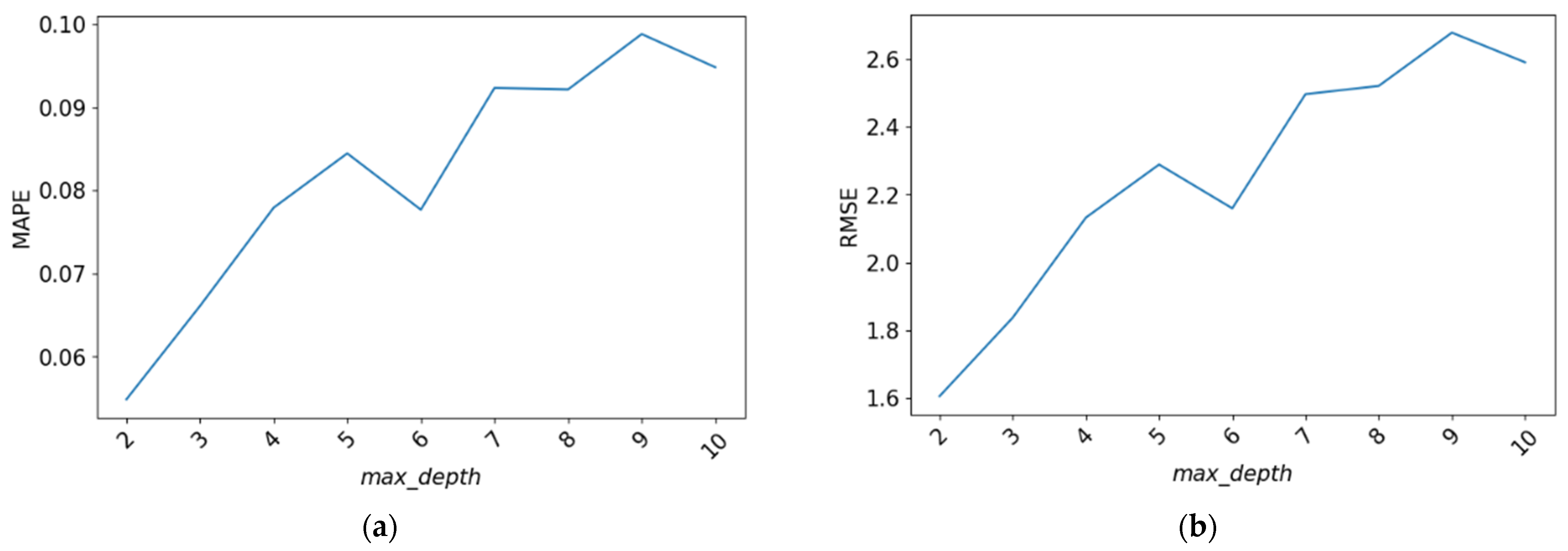
4.2.1. Max_Depth
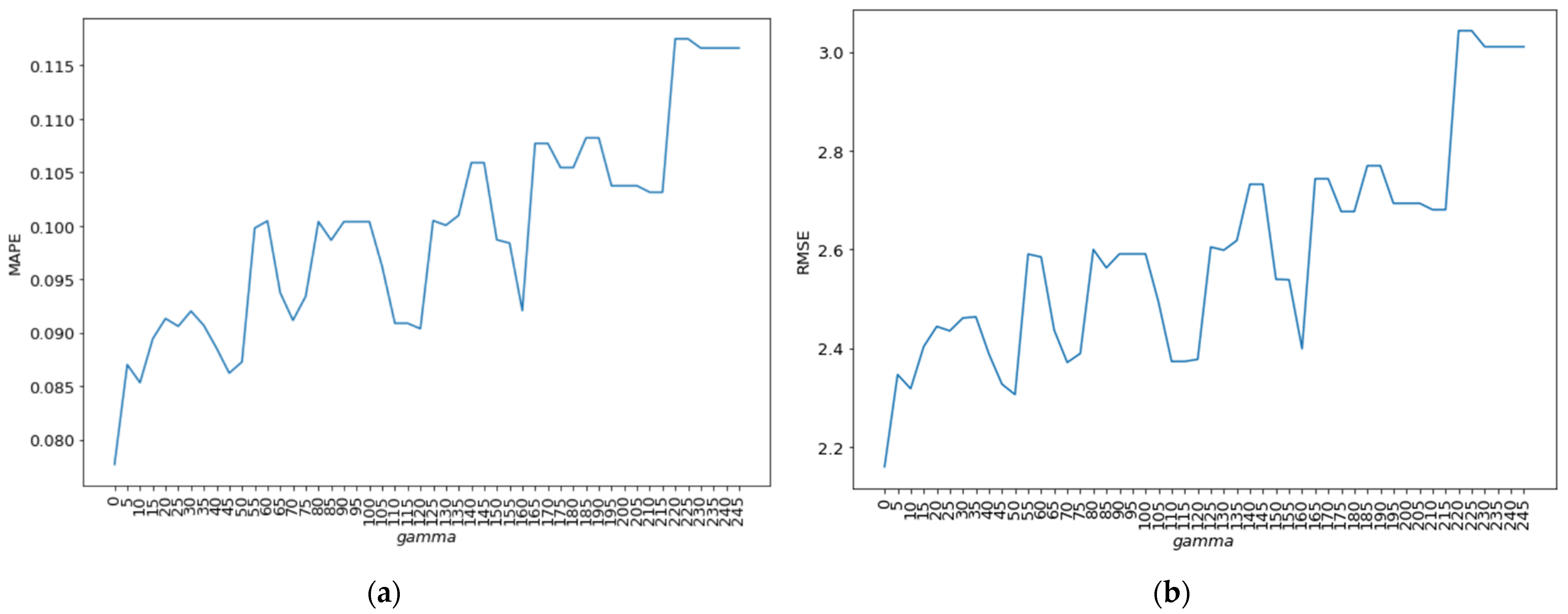
4.2.2. Gamma
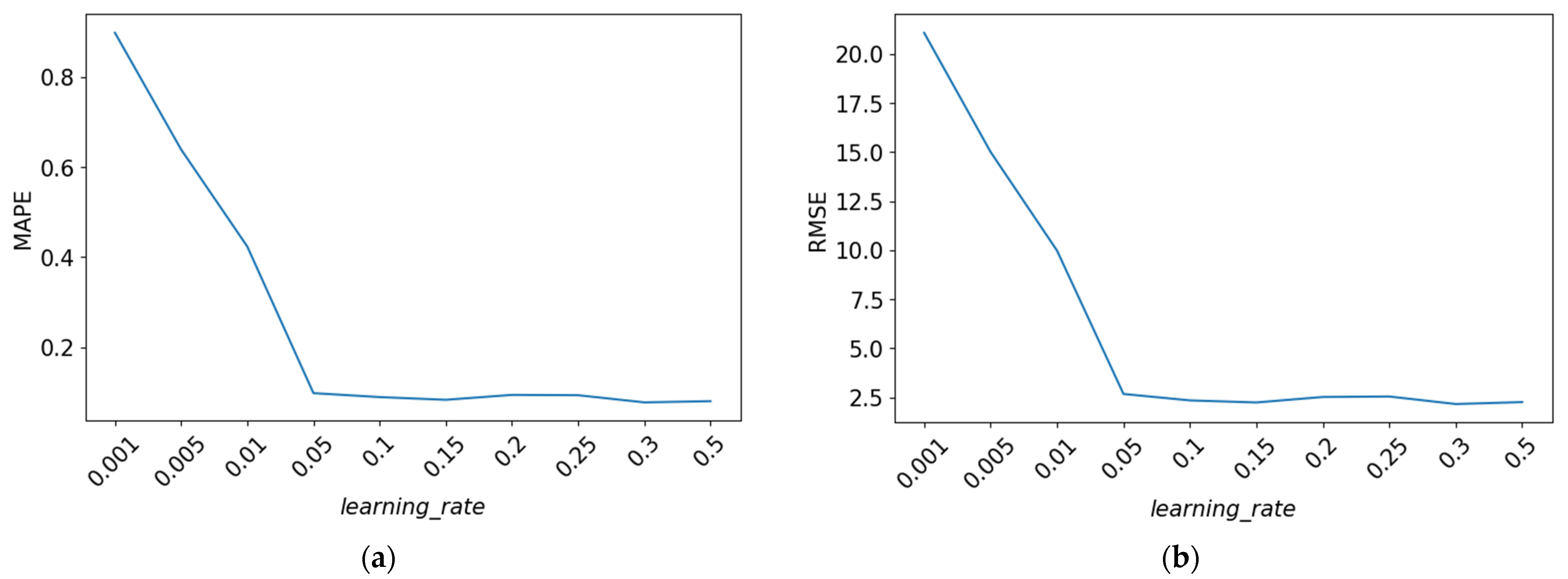
4.2.3. Learning_Rate
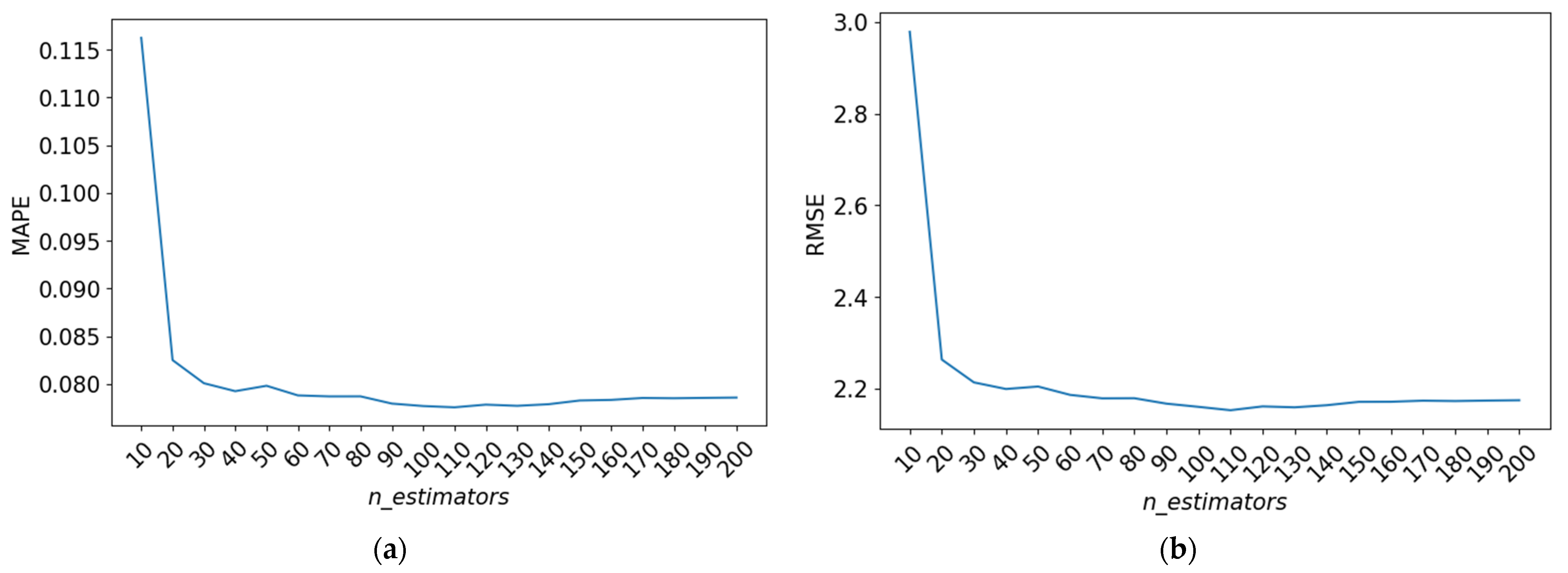
4.2.4. N_Estimators
4.2.5. Best Hyperparameter Combination
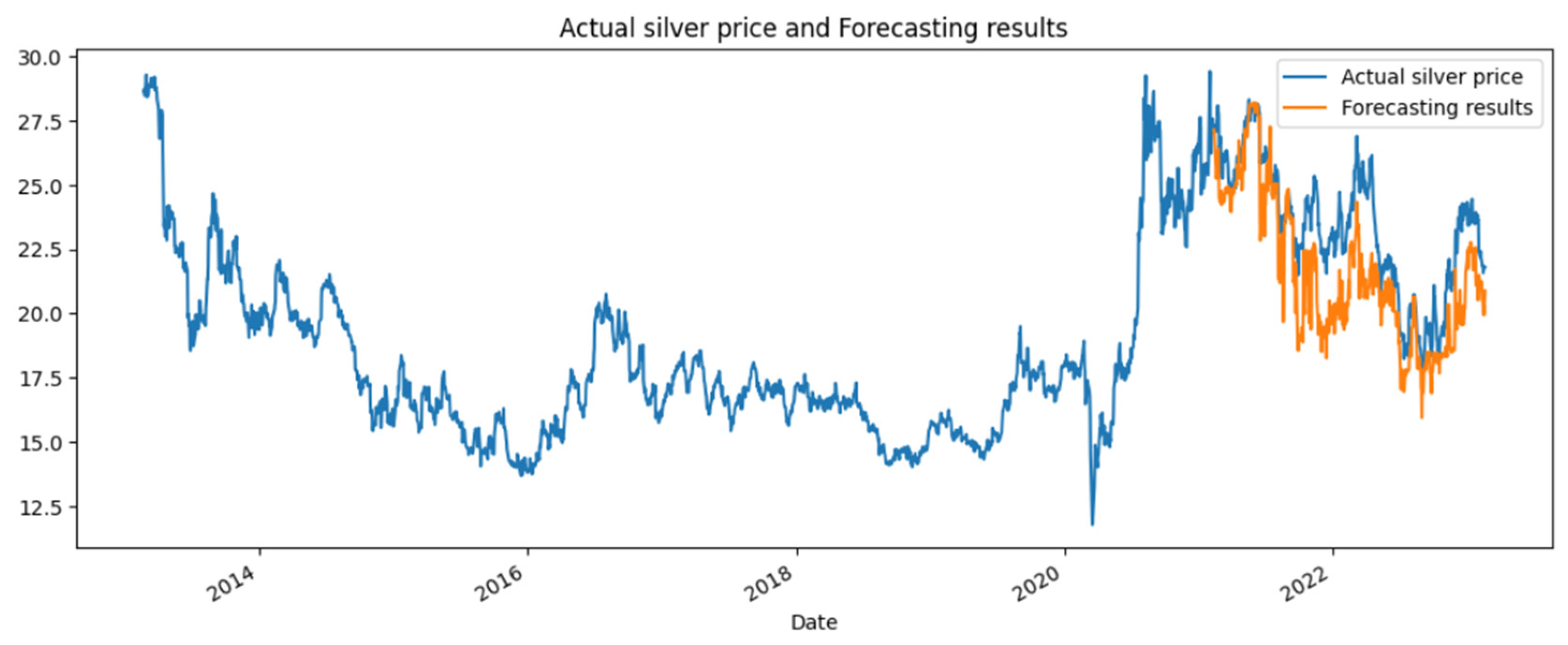
4.3. Forecasting Result
4.4. K-Fold Cross Validation
4.5. Comparison with Other Models
5. Conclusions
6. Recommendations
Author Contributions
Funding
Data Availability Statement
Conflicts of Interest
References
- Ciner, C. On the Long Run Relationship between Gold and Silver Prices A Note. Glob. Financ. J. 2001, 12, 299–303. [Google Scholar] [CrossRef]
- Lee, S.H.; Jun, B.-H. Silver Nanoparticles: Synthesis and Application for Nanomedicine. Int. J. Mol. Sci. 2019, 20, 865. [Google Scholar] [CrossRef] [PubMed]
- Dutta, A. Impact of Silver Price Uncertainty on Solar Energy Firms. J. Clean. Prod. 2019, 225, 1044–1051. [Google Scholar] [CrossRef]
- Al-Yahyaee, K.H.; Mensi, W.; Sensoy, A.; Kang, S.H. Energy, Precious Metals, and GCC Stock Markets: Is There Any Risk Spillover? Pac.-Basin Financ. J. 2019, 56, 45–70. [Google Scholar] [CrossRef]
- Hillier, D.; Draper, P.; Faff, R. Do Precious Metals Shine? An Investment Perspective. Financ. Anal. J. 2006, 62, 98–106. [Google Scholar] [CrossRef]
- O’Connor, F.A.; Lucey, B.M.; Batten, J.A.; Baur, D.G. The Financial Economics of Gold—A Survey. Int. Rev. Financ. Anal. 2015, 41, 186–205. [Google Scholar] [CrossRef]
- Jabeur, S.B.; Mefteh-Wali, S.; Viviani, J.L. Forecasting Gold Price with the XGBoost Algorithm and SHAP Interaction Values. Ann. Oper. Res. 2021. [Google Scholar] [CrossRef]
- Pierdzioch, C.; Risse, M. Forecasting Precious Metal Returns with Multivariate Random Forests. Empir. Econ. 2020, 58, 1167–1184. [Google Scholar] [CrossRef]
- Shaikh, I. On the Relation between Pandemic Disease Outbreak News and Crude Oil, Gold, Gold Mining, Silver and Energy Markets. Resour. Policy 2021, 72, 102025. [Google Scholar] [CrossRef]
- Investing.Com—Stock Market Quotes & Financial News. Available online: https://www.investing.com/ (accessed on 26 August 2023).
- Hyndman, R.J.; Athanasopoulos, G. Forecasting: Principles and Practice; OTexts, 2018. [Google Scholar]
- Divina, F.; García Torres, M.; Goméz Vela, F.A.; Vázquez Noguera, J.L. A Comparative Study of Time Series Forecasting Methods for Short Term Electric Energy Consumption Prediction in Smart Buildings. Energies 2019, 12, 1934. [Google Scholar] [CrossRef]
- Janiesch, C.; Zschech, P.; Heinrich, K. Machine Learning and Deep Learning. Electron. Mark. 2021, 31, 685–695. [Google Scholar] [CrossRef]
- Fang, Z.G.; Yang, S.Q.; Lv, C.X.; An, S.Y.; Wu, W. Application of a Data-Driven XGBoost Model for the Prediction of COVID-19 in the USA: A Time-Series Study. BMJ Open 2022, 12, e056685. [Google Scholar] [CrossRef] [PubMed]
- Chen, T.; Guestrin, C. XGBoost: A Scalable Tree Boosting System. In Proceedings of the ACM SIGKDD International Conference on Knowledge Discovery and Data Mining, San Francisco, CA, USA, 13–17 August 2016; Association for Computing Machinery: New York, NY, USA, 2016; pp. 785–794. [Google Scholar]
- Qin, C.; Zhang, Y.; Bao, F.; Zhang, C.; Liu, P.; Liu, P. XGBoost Optimized by Adaptive Particle Swarm Optimization for Credit Scoring. Math. Probl. Eng. 2021, 2021, 6655510. [Google Scholar] [CrossRef]
- Srinivasan, A.R.; Lin, Y.-S.; Antonello, M.; Knittel, A.; Hasan, M.; Hawasly, M.; Redford, J.; Ramamoorthy, S.; Leonetti, M.; Billington, J.; et al. Beyond RMSE: Do Machine-Learned Models of Road User Interaction Produce Human-like Behavior? IEEE Trans. Intell. Transp. Syst. 2023, 24, 7166–7177. [Google Scholar] [CrossRef]
- Nasiri, H.; Ebadzadeh, M.M. MFRFNN: Multi-Functional Recurrent Fuzzy Neural Network for Chaotic Time Series Prediction. Neurocomputing 2022, 507, 292–310. [Google Scholar] [CrossRef]
- Luo, M.; Wang, Y.; Xie, Y.; Zhou, L.; Qiao, J.; Qiu, S.; Sun, Y. Combination of Feature Selection and Catboost for Prediction: The First Application to the Estimation of Aboveground Biomass. Forests 2021, 12, 216. [Google Scholar] [CrossRef]
- Li, X.; Ma, L.; Chen, P.; Xu, H.; Xing, Q.; Yan, J.; Lu, S.; Fan, H.; Yang, L.; Cheng, Y. Probabilistic Solar Irradiance Forecasting Based on XGBoost. Energy Rep. 2022, 8, 1087–1095. [Google Scholar] [CrossRef]
- Qi, Y. Random Forest for Bioinformatics. Ensemble Mach. Learn. Methods Appl. 2012, 8, 307–323. [Google Scholar]
- Prokhorenkova, L.; Gusev, G.; Vorobev, A.; Dorogush, A.V.; Gulin, A. CatBoost: Unbiased Boosting with Categorical Features. Adv. Neural Inf. Process. Syst. 2018, 31, 6638–6648. [Google Scholar]
- Alruqi, M.; Hanafi, H.A.; Sharma, P. Prognostic Metamodel Development for Waste-Derived Biogas-Powered Dual-Fuel Engines Using Modern Machine Learning with K-Cross Fold Validation. Fermentation 2023, 9, 598. [Google Scholar] [CrossRef]
- Feng, D.-C.; Liu, Z.-T.; Wang, X.-D.; Chen, Y.; Chang, J.-Q.; Wei, D.-F.; Jiang, Z.-M. Machine Learning-Based Compressive Strength Prediction for Concrete: An Adaptive Boosting Approach. Constr. Build. Mater. 2020, 230, 117000. [Google Scholar] [CrossRef]
- Zhang, Y.; Li, S.; Liao, L. Input Delay Estimation for Input-Affine Dynamical Systems Based on Taylor Expansion. IEEE Trans. Circuits Syst. II Express Briefs 2020, 68, 1298–1302. [Google Scholar] [CrossRef]
- Yang, L.; Shami, A. On Hyperparameter Optimization of Machine Learning Algorithms: Theory and Practice. Neurocomputing 2020, 415, 295–316. [Google Scholar] [CrossRef]
- Probst, P.; Boulesteix, A.-L.; Bischl, B. Tunability: Importance of Hyperparameters of Machine Learning Algorithms. J. Mach. Learn. Res. 2019, 20, 1934–1965. [Google Scholar]
- Ma, Y.; Pan, H.; Qian, G.; Zhou, F.; Ma, Y.; Wen, G.; Zhao, M.; Li, T. Prediction of Transmission Line Icing Using Machine Learning Based on GS-XGBoost. J. Sens. 2022, 2022, 2753583. [Google Scholar] [CrossRef]
- Vivas, E.; Allende-Cid, H.; Salas, R. A Systematic Review of Statistical and Machine Learning Methods for Electrical Power Forecasting with Reported MAPE Score. Entropy 2020, 22, 1412. [Google Scholar] [CrossRef]
- Wang, W.; Lu, Y. Analysis of the Mean Absolute Error (MAE) and the Root Mean Square Error (RMSE) in Assessing Rounding Model. In Proceedings of the IOP Conference Series: Materials Science and Engineering, Kuala Lumpur, Malaysia, 15–16 December 2017; Volume 324, p. 12049. [Google Scholar]
- Chai, T.; Draxler, R.R. Root Mean Square Error (RMSE) or Mean Absolute Error (MAE). Geosci. Model Dev. Discuss. 2014, 7, 1525–1534. [Google Scholar]
- Mokhtar, A.; El-Ssawy, W.; He, H.; Al-Anasari, N.; Sammen, S.S.; Gyasi-Agyei, Y.; Abuarab, M. Using Machine Learning Models to Predict Hydroponically Grown Lettuce Yield. Front. Plant Sci. 2022, 13, 706042. [Google Scholar] [CrossRef]
- Gareth, J.; Daniela, W.; Trevor, H.; Robert, T. An Introduction to Statistical Learning: With Applications in R; Spinger: Berlin/Heidelberg, Germany, 2013. [Google Scholar]
- Marzban, C.; Liu, J.; Tissot, P. On Variability Due to Local Minima and K-Fold Cross Validation. Artif. Intell. Earth Syst. 2022, 1, e210004. [Google Scholar] [CrossRef]
- Elasra, A. Multiple Imputation of Missing Data in Educational Production Functions. Computation 2022, 10, 49. [Google Scholar] [CrossRef]


| Silver Price | Gold Price | Platinum Price | USD/EUR | |
|---|---|---|---|---|
| Mean | 19.11 | 1441.03 | 1048.56 | 0.8637 |
| Median | 17.82 | 1318.50 | 979.75 | 0.8797 |
| Std. Dev | 3.80 | 260.60 | 208.44 | 0.0664 |
| Maximum | 29.42 | 2069.40 | 1624.80 | 1.0421 |
| Minimum | 11.77 | 1049.60 | 595.20 | 0.7177 |
| Count | 2566 | 2566 | 2566 | 2566 |
| Hyperparameter | Description | Default Value |
|---|---|---|
| learning_rate | A hyperparameter that sets the step size shrinkage in the output value update | 0.3 |
| max_depth | A hyperparameter that sets the maximum depth of the tree | 6 |
| n_estimators | Hyperparameters that set the maximum number of trees | 100 |
| gamma | A hyperparameter that sets the minimum required branching constraint for each node | 0 |
| Learning_Rate | Max_Depth | N_Estimators | Gamma | MAPE (%) |
|---|---|---|---|---|
| 0.15 | 2 | 130 | 0 | 5.982 |
| 0.1 | 3 | 130 | 0 | 6.0558 |
| 0.15 | 2 | 100 | 0 | 6.0993 |
| Learning_Rate | Max_Depth | N_Estimators | Gamma | RMSE |
|---|---|---|---|---|
| 0.1 | 3 | 130 | 0 | 1.6967 |
| 0.15 | 2 | 130 | 0 | 1.6998 |
| 0.15 | 2 | 100 | 0 | 1.7277 |
| Date | Silver Price ($) (Model A) | Silver Price ($) (Model B) |
|---|---|---|
| 21 February 2023 | 21.7131 | 21.8824 |
| 22 February 2023 | 21.5283 | 20.8134 |
| 23 February 2023 | 21.9233 | 19.6417 |
| 24 February 2023 | 20.2312 | 20.8694 |
| 27 February 2023 | 21.7131 | 21.8824 |
| 28 February 2023 | 21.7131 | 21.8862 |
| Iteration | Model A | Model B | ||
|---|---|---|---|---|
| MAPE | RMSE | MAPE | RMSE | |
| 1 | 8.64% | 2.6586 | 7.45% | 2.36 |
| 2 | 4.23% | 0.8678 | 4.8% | 1.0121 |
| 3 | 5.78% | 1.1849 | 4.51% | 0.9577 |
| 4 | 15.37% | 3.1645 | 15.53% | 3.1704 |
| 5 | 5.98% | 1.6998 | 6.06% | 1.6967 |
| Average | 8% | 1.9151 | 7.67% | 1.8394 |
| Model | Average MAPE | Average RMSE |
|---|---|---|
| Model B | 7.67% | 1.8394 |
| Model A | 8% | 1.9151 |
| Models | RMSE | MAPE | MAE | SI |
|---|---|---|---|---|
| Proposed model A | 1.6998 | 0.0598 | 1.4051 | 0.0729 |
| Proposed model B | 1.6968 | 0.0606 | 1.4014 | 0.0728 |
| Random forest | 1.9745 | 0.0749 | 1.7288 | 0.0847 |
| XGBoost (initial) | 2.1600 | 0.0777 | 1.8001 | 0.0926 |
| CatBoost | 2.1689 | 0.0859 | 1.9776 | 0.0930 |
Disclaimer/Publisher’s Note: The statements, opinions and data contained in all publications are solely those of the individual author(s) and contributor(s) and not of MDPI and/or the editor(s). MDPI and/or the editor(s) disclaim responsibility for any injury to people or property resulting from any ideas, methods, instructions or products referred to in the content. |
© 2023 by the authors. Licensee MDPI, Basel, Switzerland. This article is an open access article distributed under the terms and conditions of the Creative Commons Attribution (CC BY) license (https://creativecommons.org/licenses/by/4.0/).
Share and Cite
Gono, D.N.; Napitupulu, H.; Firdaniza. Silver Price Forecasting Using Extreme Gradient Boosting (XGBoost) Method. Mathematics 2023, 11, 3813. https://doi.org/10.3390/math11183813
Gono DN, Napitupulu H, Firdaniza. Silver Price Forecasting Using Extreme Gradient Boosting (XGBoost) Method. Mathematics. 2023; 11(18):3813. https://doi.org/10.3390/math11183813
Chicago/Turabian StyleGono, Dylan Norbert, Herlina Napitupulu, and Firdaniza. 2023. "Silver Price Forecasting Using Extreme Gradient Boosting (XGBoost) Method" Mathematics 11, no. 18: 3813. https://doi.org/10.3390/math11183813
APA StyleGono, D. N., Napitupulu, H., & Firdaniza. (2023). Silver Price Forecasting Using Extreme Gradient Boosting (XGBoost) Method. Mathematics, 11(18), 3813. https://doi.org/10.3390/math11183813