Study of a New Software Reliability Growth Model under Uncertain Operating Environments and Dependent Failures

Abstract

The coronavirus disease (COVID-19) outbreak has prompted various industries to embark on digital transformation efforts, with software playing a critical role. Ensuring the reliability of software is of the utmost importance given its widespread use across multiple industries. For example, software has extensive applications in areas such as transportation, aviation, and military systems, where reliability problems can result in personal injuries and significant financial losses. Numerous studies have focused on software reliability. In particular, the software reliability growth model has served as a prominent tool for measuring software reliability. Previous studies have often assumed that the testing environment is representative of the operating environment and that software failures occur independently. However, the testing and operating environments can differ, and software failures can sometimes occur dependently. In this study, we propose a new model that assumes uncertain operating environments and dependent failures. In other words, the model proposed in this study takes into account a wider range of environments. The numerical examples in this study demonstrate that the goodness of fit of the new model is significantly better than that of the existing SRGM. Additionally, we show the utilization of the sequential probability ratio test (SPRT) based on the new model to assess the reliability of the dataset.

1. Introduction

A software reliability growth model (SRGM) is employed to assess the reliability and quality of software products. This enables consumers to evaluate products by referring to reliability information, and developers can efficiently manage development plans based on reliability considerations. For instance, using the mean value function m(t), it is possible to predict the number of failures at a future time point t. Additionally, it can be used to establish policies for determining the optimal release timing for selling products. In other words, the SRGM is used as a tool for predicting the number of failures in future time periods, predicting product reliability, determining release policies, and estimating development costs. A software reliability growth model is represented by a mean value function m(t) that exhibits unique characteristics. The form of m(t) varies depending on the assumed environments (such as the development, testing, and operating phases). Although there have been numerous studies on software reliability models, it is generally observed that software defects and failures do not occur at regular time intervals. In response to this, existing SRGMs predominantly adopt a nonhomogeneous Poisson process (NHPP) framework. NHPP SRGMs provide a mathematical framework for handling software reliability and are widely utilized due to their versatility in various applications. Previous NHPP software reliability models were primarily built on the assumptions that any faults detected during the testing phase are promptly resolved without any debugging delays, no new faults are introduced, and the software systems deployed in real-world environments are either identical to or closely resemble those used during development and testing.

Most SRGMs generally follow a NHPP and assume that the testing environments are the same as the operating environments, and failures occur independently. In addition, SRGM modeling studies consider assumptions such as debugging environments, testing coverage function, total number of faults, and fault detection rate function. Huang et al. [1] introduced an NHPP SRGM that considered imperfect debugging, various errors, and change-points during the testing phase. Lou et al. [2] discussed a generalized NHPP SRGM with imperfect debugging. Imperfect debugging refers to the state in which not all faults or bugs within the software are eliminated when they occur. Chiu et al. [3] proposed an SRGM in which the number of potential errors fluctuates throughout the debugging period. Gupta et al. [4] introduced a model that considered the coverage factor and power functions in development environments. Zhang et al. [5] proposed a model that introduced new errors during the debugging period owing to imperfect debugging. Nguyen et al. [6] developed a new NHPP SRGM with an S-shaped fault detection rate function having three parameters.

Uncertain operating environments refer to the actual environment in which consumers use the software, including factors such as the operating system, background environments, hardware specifications, etc. This encompasses various scenarios and possibilities. Pradhan et al. [7,8,9,10] developed a model that incorporated an S-shaped inflection as the testing coverage function and considered uncertain operating environments. Environment factors (EFs) refer to various internal and external environments such as testing environments, programming tools, programming effort, program structure, hardware specifications, etc. The testing environment is also not consistent. Haque et al. [11] considered uncertain testing environments such as testing effort, testing skills, and testing coverage. Chatterjee et al. [12] studied the randomness effort using uncertain testing environments and operating environments. The NHPP SRGM studies mentioned earlier assumed independent failures. Sometimes, software failures can occur dependently due to interactions among EFs. Lee et al. [13] and Kim et al. [14] assumed that failures occurred dependently.

SRGMs can be used not only to determine reliability but also to plan release or warranty policies. Raheem et al. [15] devised an optimal release policy based on an SRGM considering imperfect debugging. Minamino et al. [16] and Ke et al. [17] introduced an optimal release policy based on a change-point model. Several studies have been conducted on software reliability using various approaches. Saxena et al. [18], Kumar et al. [19], and Garg et al. [20] developed criteria to assess the goodness of fit of SRGMs. These criteria were derived from a combination of the entropy principle and existing evaluation measures. Several studies have focused on criteria evaluating the reliability of the software and hardware. Yaghoobi [21] proposed two multicriteria decision-making methods for comparing SRGMs. Zhu [22] introduced the concept of complex reliability, which considered both hardware and software components, and proposed maintenance policies applicable to such systems. Several recent software reliability studies have employed machine-learning and deep-learning techniques [23,24,25,26].

Hypothesis testing is worth considering to determine software reliability. However, classical hypothesis testing requires large datasets, which is often a limitation because most software failure datasets are small. To address this issue, we introduce the sequential probability ratio test (SPRT) pioneered by Wald [27], which enables testing with small datasets. Unlike traditional statistical hypothesis testing, the SPRT provides test results at each data collection point, saving time and reducing the cost of data collection by drawing conclusions with less data. In other words, the SPRT is an efficient hypothesis-testing method in terms of time and cost. Stieber [28] successfully applied Wald’s SPRT to ensure software reliability. In this study, we extend the SPRT methodology to estimate software reliability.

The aim of this study is as follows: First, we present a new SRGM that considers both uncertain operating environments and dependent failures. Most of the SRGM research assumes either uncertain operating environments or only considers fault dependency. However, in this study, we develop a model that takes both assumptions into account. Subsequently, we evaluate the performance of each model using real datasets. Numerical examples demonstrate that the proposed model outperforms other models that solely account for uncertain operating environments or dependent failures. This provides a more accurate prediction of the number of failures. Additionally, we demonstrate the effectiveness of the SPRT by utilizing optimal assumption cases based on our proposed model. This allows testers to determine when to stop testing based on the software reliability.

In Section 2, we provide the basic background of NHPP SRGMs and introduce the existing NHPP SRGM models as well as the model proposed in this paper. The SPRT procedure is outlined in Section 3. Section 4 presents the datasets and criteria used in this numerical study. We compare the fit of each model to the datasets and apply the SPRT. In Section 5, we discuss the results of the numerical example. Finally, Section 6 presents the conclusions of this study.

2. Software Reliability Growth Model

2.1. Nonhomogeneous Poisson Process

Most SRGMs assume the nonhomogeneous Poisson process (NHPP), which can be represented by the following equation:

$$\mathrm{Pr}\left\{\mathrm{N}\left(\mathrm{t}\right)=\mathrm{n}\right\}=\frac{\{{\mathrm{m}\left(\mathrm{t}\right)\}}^{\mathrm{n}}}{\mathrm{n}!}{\mathrm{e}}^{-\mathrm{m}\left(\mathrm{t}\right)},\mathrm{n}=0,1,2,3,\dots .$$

(1)

It characterizes the cumulative number of failures, denoted as $\mathrm{N}\left(\mathrm{t}\right)(\mathrm{t}\ge 0)$, up to a given execution time t. The mean value function m(t) represents the expected cumulative number of failures at time t. The function m(t) can be obtained by integrating the intensity function $\mathsf{\lambda }\left(\mathrm{t}\right)$ from 0 to t as follows:

$$\mathrm{m}\left(\mathrm{t}\right)={\int }_0^{\mathrm{t}}\mathsf{\lambda }\left(\mathrm{s}\right)\mathrm{d}\mathrm{s}.$$

(2)

The reliability function based on the NHPP can be expressed as follows using m(t) [29]. The reliability function R(t) is defined as the probability that there are no failures in the time interval (0, t), given by

$$\mathrm{R}\left(\mathrm{t}\right)=\mathrm{P}\left\{\mathrm{N}\left(\mathrm{t}\right)=0\right\}={\mathrm{e}}^{-\mathrm{m}\left(\mathrm{t}\right)}.$$

(3)

Equation (3) means the probability that a software error does not occur in the interval (0, t). If t + x is given, then the software reliability can be expressed as a conditional probability $\mathrm{R}\left(\mathrm{x}\right|\mathrm{t})$ as in Equation (4).

$$\mathrm{R}\left(\mathrm{x}|\mathrm{t}\right)=\mathrm{P}\left\{\mathrm{N}\left(\mathrm{t}+\mathrm{x}\right)-\mathrm{N}\left(\mathrm{t}\right)=0\right\}={\mathrm{e}}^{-[\mathrm{m}\left(\mathrm{t}+\mathrm{x}\right)-\mathrm{m}(\mathrm{t}\left)\right]}$$

(4)

Here, $\mathrm{R}\left(\mathrm{x}\right|\mathrm{t})$ is the probability that a software error does not occur in the interval (t, t + x), where $\mathrm{t}\ge 0$, $\mathrm{x}>0$. The density function of x is given by

$$\mathrm{f}\left(\mathrm{x}\right)=\mathsf{\lambda }(\mathrm{t}+\mathrm{x}){\mathrm{e}}^{-[\mathrm{m}\left(\mathrm{t}+\mathrm{x}\right)-\mathrm{m}(\mathrm{t}\left)\right]}$$

(5)

where $\mathsf{\lambda }\left(\mathrm{x}\right)=\frac{\partial }{\partial \mathrm{x}}\left[\mathrm{m}\right(\mathrm{x}\left)\right]$.

2.2. Existing SRGMs

The mean value function m(t) of the NHPP SRGM is obtained by solving a differential equation. The form of the mean value function depends on the assumptions and specific environments being studied. The commonly used differential equation is as follows [30]:

$$\frac{\mathrm{d}\mathrm{m}\left(\mathrm{t}\right)}{\mathrm{d}\mathrm{t}}=\mathrm{b}\left(\mathrm{t}\right)\left[\mathrm{a}\left(\mathrm{t}\right)-\mathrm{m}\left(\mathrm{t}\right)\right]$$

(6)

where the function $\mathrm{a}\left(\mathrm{t}\right)$ and represents the expected number of initial failures and newly introduced errors until the start point of testing period and $\mathrm{b}\left(\mathrm{t}\right)$ represents the failure detection rate per fault.

This paper presents a specific software reliability model with consideration of the uncertainty of the operating environment based on the work by Pham [26].

The NHPP SRGM is typically characterized by a differential equation that is widely recognized in the field. To account for the uncertain operating conditions considered in this study, the mean value function of the proposed model is obtained as follows [31]:

$$\frac{\mathrm{m}\left(\mathrm{t}\right)}{\mathrm{d}\mathrm{t}}=\mathsf{\eta }\mathrm{b}\left(\mathrm{t}\right)\left[\mathrm{a}\left(\mathrm{t}\right)-\mathrm{m}\left(\mathrm{t}\right)\right]$$

(7)

where η is a random variable. In order to explain the uncertain operating environment, this equation utilizes the random variable η, which has a $\mathsf{\Gamma }(\mathsf{\alpha },\mathsf{\beta })$.

2.3. Proposed Model

Most existing NHPP SRGMs assume that testing and operating environments are the same and that failures occur independently. However, sometimes software failures occur dependently, and the operating environments may differ from the testing environments. For example, if an error occurs in a particular class within a program code, then it may cause errors in other classes that refer to the affected class. Conflicts between program codes due to background processes can potentially impact other codes. These situations lead to the occurrence of dependent failures. Furthermore, constructing a testing environments that consider all operating environments is difficult for testers. The operating environment means the environment in which consumers use the software, including hardware specifications (CPU, GPU, RAM, etc.), operating systems (Window, Mac, Linux, etc.), and various concurrently running programs in the background. The proposed model considers dependent failures and uncertain operating environments. Quantifying the operating environments numerically is difficult. So, looking at Equation (7), the uncertain operating environments are represented by η, the random variable. The assumption of dependent failure occurrences is represented by the parameters of the gamma distribution followed by η, which will be discussed in detail when explaining Equation (10).

In this paper, we propose a model that incorporates both uncertain operating environments and dependent failures. The inclusion of the latter is motivated by the need to consider situations in which failures can propagate from one component to another. With the functions $\mathrm{a}\left(\mathrm{t}\right)=\mathrm{N}$ and $\mathrm{b}\left(\mathrm{t}\right)=\mathrm{c}/(1+\mathsf{\alpha }\exp \left(-\mathrm{b}\mathrm{t}\right))$, we can obtain the mean value function m(t) from Equation (7), as shown below:

$$\mathrm{m}\left(\mathrm{t}\right)=\int \mathrm{N}\left(1-{\mathrm{e}}^{-\mathsf{\eta }{\int }_0^{\mathrm{t}}\mathrm{b}\left(\mathrm{s}\right)\mathrm{d}\mathrm{s}}\right)\mathrm{d}\mathrm{g}\left(\mathsf{\eta }\right),$$

(8)

$$\mathrm{m}\left(\mathrm{t}\right)=\mathrm{N}{\left(1-\frac{\mathsf{\beta }}{\mathsf{\alpha }+\int \mathrm{b}\left(\mathrm{s}\right)\mathrm{d}\mathrm{s}}\right)}^{\mathsf{\alpha }}=\mathrm{N}{\left(1-\frac{\mathsf{\beta }}{\mathsf{\alpha }+{\int }_0^{\mathrm{t}}\frac{\mathrm{c}}{1+\mathsf{\alpha }{\mathrm{e}}^{-\mathrm{b}\mathrm{s}}}\mathrm{d}\mathrm{s}}\right)}^{\mathsf{\alpha }}$$

(9)

$$=\mathrm{N}{\left(1-\frac{\mathsf{\beta }}{\mathsf{\alpha }+\frac{\mathrm{c}}{\mathrm{b}}\mathrm{l}\mathrm{n}\left(\frac{\mathsf{\alpha }+{\mathrm{e}}^{\mathrm{b}\mathrm{t}}}{1+\mathsf{\alpha }}\right)}\right)}^{\mathsf{\alpha }}$$

(10)

The proposed model has five parameters, namely b, c, α, β, and N. In Equation (10), the parameters α and β are also the parameters of $\mathrm{g}\left(\mathsf{\eta }\right)=\frac{{\mathsf{\beta }}^{\mathsf{\alpha }}{\mathsf{\eta }}^{\mathsf{\alpha }-1}{\mathrm{e}}^{-\mathsf{\beta }\mathsf{\eta }}}{\mathsf{\Gamma }\left(\mathsf{\alpha }\right)}$, which is the gamma distribution, where η represents the uncertain operating environments in Equation (7).

The assumption of dependent failures in the proposed model arises from the interdependence of model parameters. Specifically, the values of $\mathsf{\alpha }$ and $\mathsf{\beta }$ in Equation (10) depend on the probability distribution of η, which characterizes the uncertain operating environments. As these parameters appear in Equation (7), which expresses the failure detection rate, the assumption of dependent failures is a natural consequence of the model design. Therefore, the correlation between model parameters is a crucial factor that underlies the assumption of dependent failures.

Table 1. Mean value functions for the existing NHPP SRGMs and the proposed model.

No.	Model	$\mathbf{m}\left(\mathbf{t}\right)$
1	DPF1 [13] (dependent failure model 1)	$\frac{\mathrm{a}}{1+\left(\frac{\mathrm{a}}{\mathrm{h}}{\left(\frac{\mathrm{b}+\mathrm{c}}{\mathrm{c}+\left(\mathrm{b}\exp \left(\mathrm{b}\mathrm{t}\right)\right)}\right)}^{\frac{\mathrm{a}}{\mathrm{b}}}\right)}$	$\mathrm{a}\left(\mathrm{t}\right)=\mathrm{a}$ $\mathrm{b}\left(\mathrm{t}\right)=\frac{\mathrm{b}}{1+\mathrm{c}{\mathrm{e}}^{-\mathrm{b}\mathrm{t}}}$
2	DPF2 [14] (dependent failure model 2)	$\frac{\mathrm{a}}{1+\left(\frac{\mathrm{a}}{\mathrm{h}}{\left(\frac{1+\mathrm{c}}{\mathrm{c}+\exp \left(\mathrm{b}\mathrm{t}\right)}\right)}^{\mathrm{a}}\right)}$	$\mathrm{a}\left(\mathrm{t}\right)=\mathrm{N}$ $\mathrm{b}\left(\mathrm{t}\right)=\frac{{\mathrm{b}}^2\mathrm{t}}{1+\mathrm{b}\mathrm{t}}$
3	DS [32] (delayed S-shaped model)	$\mathrm{a}\left(1-\left(1+\mathrm{b}\mathrm{t}\right)\exp \left(-\mathrm{b}\mathrm{t}\right)\right)$	$\mathrm{a}\left(\mathrm{t}\right)=\mathrm{a}$ $\mathrm{b}\left(\mathrm{t}\right)=\frac{{\mathrm{b}}^2\mathrm{t}}{1+\mathrm{b}\mathrm{t}}$
4	GO [33] (by Goel–Okumoto)	$\mathrm{a}\left(1-\exp \left(-\mathrm{b}\mathrm{t}\right)\right)$	$\mathrm{a}\left(\mathrm{t}\right)=\mathrm{a}$ $\mathrm{b}\left(\mathrm{t}\right)=\mathrm{b}$
5	IS [34] (inflection S-shaped model)	$\frac{\mathrm{a}\left(1-\exp \left(-\mathrm{b}\mathrm{t}\right)\right)}{1+\mathsf{\beta }\exp \left(-\mathrm{b}\mathrm{t}\right)}$	$\mathrm{a}\left(\mathrm{t}\right)=\mathrm{a}$ $\mathrm{b}\left(\mathrm{t}\right)=\frac{\mathrm{b}}{1+\mathsf{\beta }{\mathrm{e}}^{-\mathrm{b}\mathrm{t}}}$
6	YID [35] (imperfect debugging model by Yamada)	$\mathrm{a}\left(1-\exp \left(-\mathrm{b}\mathrm{t}\right)\right)\left(1-\frac{\mathsf{\alpha }}{\mathrm{b}}\right)+\mathsf{\alpha }\mathrm{a}\mathrm{t}$	$\mathrm{a}\left(\mathrm{t}\right)=\mathrm{a}(1+\mathsf{\alpha }\mathrm{t})$ $\mathrm{b}\left(\mathrm{t}\right)=\mathrm{b}$
7	PNZ [30] (by Pham–Nordmann–Zhang)	$\frac{\mathrm{a}\left(1-\exp \left(-\mathrm{b}\mathrm{t}\right)\right)\left(1-\frac{\mathsf{\alpha }}{\mathrm{b}}\right)+\mathsf{\alpha }\mathrm{a}\mathrm{t}}{1+\left(\mathsf{\beta }\exp \left(-\mathrm{b}\mathrm{t}\right)\right)}$	$\mathrm{a}\left(\mathrm{t}\right)=\mathrm{a}(1+\mathsf{\alpha }\mathrm{t})$ $\mathrm{b}\left(\mathrm{t}\right)=\frac{\mathrm{b}}{1+\mathsf{\beta }{\mathrm{e}}^{-\mathrm{b}\mathrm{t}}}$
8	PZ [36] (by Pham–Zhang)	$\frac{\left(\left(\mathrm{c}+\mathrm{a}\right)\left(1-\exp \left(-\mathrm{b}\mathrm{t}\right)\right)\right)-\left(\frac{\mathrm{a}\mathrm{b}}{\mathrm{b}-\mathsf{\alpha }}\left(\exp \left(-\mathrm{a}\mathrm{t}\right)-\exp \left(-\mathrm{b}\mathrm{t}\right)\right)\right)}{1+\left(\mathsf{\beta }\exp \left(-\mathrm{b}\mathrm{t}\right)\right)}$	$\mathrm{a}\left(\mathrm{t}\right)=\mathrm{c}+\mathrm{a}(1-{\mathrm{e}}^{\mathsf{\alpha }\mathrm{t}})$ $\mathrm{c}\left(\mathrm{t}\right)=\frac{\mathrm{b}}{1+\mathsf{\beta }{\mathrm{e}}^{-\mathrm{b}\mathrm{t}}}$
9	TC [37] (testing coverage model)	$\mathrm{N}\left(1-{\left(\frac{\mathsf{\beta }}{\mathsf{\beta }+{\left(\mathrm{a}\mathrm{t}\right)}^{\mathrm{b}}}\right)}^{\mathsf{\alpha }}\right)$	$\mathrm{a}\left(\mathrm{t}\right)=\mathrm{N}$ $\mathrm{c}\left(\mathrm{t}\right)=1-{\mathrm{e}}^{-{\left(\mathrm{a}\mathrm{t}\right)}^{\mathrm{b}}}$
10	VTUB [31] (VTUB model)	$\mathrm{N}\left(1-{\left(\frac{\mathsf{\beta }}{\mathsf{\beta }+\left({\mathrm{a}}^{{\mathrm{t}}^{\mathrm{b}}}\right)-1}\right)}^{\mathsf{\alpha }}\right)$	$\mathrm{a}\left(\mathrm{t}\right)=\mathrm{N}$ $\mathrm{b}\left(\mathrm{t}\right)=\mathrm{b}\ln \left(\mathrm{a}\right){\mathrm{t}}^{\mathrm{b}-1}{\mathrm{a}}^{{\mathrm{t}}^{\mathrm{b}}}$
11	NEW	$\mathrm{N}{\left(1-\frac{\mathsf{\beta }}{\mathsf{\alpha }+\frac{\mathrm{c}}{\mathrm{b}}\mathrm{l}\mathrm{n}\left(\frac{\mathsf{\alpha }+{\mathrm{e}}^{\mathrm{b}\mathrm{t}}}{1+\mathsf{\alpha }}\right)}\right)}^{\mathsf{\alpha }}$	$\mathrm{a}\left(\mathrm{t}\right)=\mathrm{N}$ $\mathrm{b}\left(\mathrm{t}\right)=\frac{\mathrm{c}}{1+\mathsf{\alpha }{\mathrm{e}}^{-\mathrm{b}\mathrm{t}}}$

lists the mean value functions for the existing NHPP SRGMs and the proposed model. Each model is referred to by abbreviations of its characteristics or author names. DPF1 and DPF2 assume dependent failures, whereas the others assume independent failures. VTUB assumes uncertain operating environments, whereas the proposed model (NEW) assumes dependent failures and uncertain operating environments.

3. Sequential Probability Ratio Test

Wald’s SPRT is widely used as a hypothesis-testing technique [27]. It tests the probability ratios of two hypotheses, ${\mathrm{p}}_0$ and ${\mathrm{p}}_1$, against a predetermined threshold value at each time point. The SPRT algorithm is iterative and requires additional data collection and testing if the probability ratio falls within a certain acceptance region (A and B). Equation (11) expresses the relationship between ${\mathrm{p}}_0$ and ${\mathrm{p}}_1$ and the thresholds A and B.

$$\mathrm{B}<\frac{{\mathrm{p}}_1}{{\mathrm{p}}_0}<\mathrm{A}$$

(11)

where $\mathrm{A}$ and $\mathrm{B}$ are constants used to determine the acceptance and rejection of the null hypothesis ${\mathrm{H}}_0$. If ${\mathrm{p}}_1/{\mathrm{p}}_0\ge \mathrm{A}$, then ${\mathrm{H}}_0$ is rejected. If ${\mathrm{p}}_1/{\mathrm{p}}_0\le \mathrm{B}$, then ${\mathrm{H}}_0$ is accepted.

Moreover, A and B depend on $\mathsf{\alpha }$ and $\mathsf{\beta }$, as shown in Equations (11) and (12). Here, $\mathsf{\alpha }$ and β are type 1 and type 2 errors, respectively. In other words, $\mathsf{\alpha }$ is the producer’s risk, and $\mathsf{\beta }$ is the consumer’s risk.

$$1-\mathsf{\beta }\ge \mathrm{A}\mathsf{\alpha },\mathsf{\beta }\le \left(1-\mathsf{\alpha }\right)\mathrm{B}$$

(12)

$$\mathrm{A}\le \frac{1-\mathsf{\beta }}{\mathsf{\alpha }},\mathrm{B}\ge \frac{\mathsf{\beta }}{1-\mathsf{\alpha }}$$

(13)

The values of A and B depend on the prespecified risk probabilities, α and β, which represent type 1 (producer’s risk) and type 2 (consumer’s risk) errors and are typically set to 0.05 or 0.1, respectively. The upper line that determines rejection is called ${\mathrm{N}}_{\mathrm{U}}\left(\mathrm{t}\right)$, and the lower line that determines acceptance is called ${\mathrm{N}}_{\mathrm{L}}\left(\mathrm{t}\right)$ are represented as follows:

$${\mathrm{N}}_{\mathrm{L}}\left(\mathrm{t}\right)=\mathrm{a}\mathrm{t}-{\mathrm{b}}_1,{\mathrm{N}}_{\mathrm{U}}\left(\mathrm{t}\right)=\mathrm{a}\mathrm{t}+{\mathrm{b}}_2.$$

(14)

where $\mathrm{a}$, ${\mathrm{b}}_1$, and ${\mathrm{b}}_2$ are given as follows

$$\mathrm{a}=\frac{\left({\mathsf{\lambda }}_1-{\mathsf{\lambda }}_0\right)}{\ln \left(\frac{{\mathsf{\lambda }}_1}{{\mathsf{\lambda }}_0}\right)},{\mathrm{b}}_1=\frac{\ln \left(\frac{1-\mathsf{\alpha }}{\mathsf{\beta }}\right)}{\ln \left(\frac{{\mathsf{\lambda }}_1}{{\mathsf{\lambda }}_0}\right)},{\mathrm{b}}_2=\frac{\ln \left(\frac{1-\mathsf{\beta }}{\mathsf{\alpha }}\right)}{\ln \left(\frac{{\mathsf{\lambda }}_1}{{\mathsf{\lambda }}_0}\right)}$$

(15)

Figure 1 shows the reliable region of SPRT. If the data value (blue dot) at a certain time point exists within the reliable region, then it is labeled as “Continue”. If the value is outside the region, then a conclusion of “Reject” or “Accept” is made.

Stieber [28] applied the SPRT to estimate the reliability of NHPP SRGMs, which involved redefining the probability ratios ${\mathrm{p}}_0$ and ${\mathrm{p}}_1$ of Equation (11) in terms of the mean value function m(t). Here, ${\mathrm{p}}_0$ and ${\mathrm{p}}_1$ are expressed as follows:

$${\mathrm{p}}_0=\frac{{\mathrm{e}}^{-{\mathrm{m}}_0\left(\mathrm{t}\right)}{\left[{\mathrm{m}}_0\left(\mathrm{t}\right)\right]}^{\mathrm{N}\left(\mathrm{t}\right)}}{\mathrm{N}\left(\mathrm{t}\right)!},{\mathrm{p}}_1=\frac{{\mathrm{e}}^{-{\mathrm{m}}_1\left(\mathrm{t}\right)}{\left[{\mathrm{m}}_1\left(\mathrm{t}\right)\right]}^{\mathrm{N}\left(\mathrm{t}\right)}}{\mathrm{N}\left(\mathrm{t}\right)!},$$

(16)

$$\frac{\ln \left(\frac{\mathsf{\beta }}{1-\mathsf{\alpha }}\right)+{\mathrm{m}}_1\left(\mathrm{t}\right)-{\mathrm{m}}_0\left(\mathrm{t}\right)}{\ln {\mathrm{m}}_1\left(\mathrm{t}\right)-\ln {\mathrm{m}}_0\left(\mathrm{t}\right)}<\mathrm{N}\left(\mathrm{t}\right)<\frac{\ln \left(\frac{1-\mathsf{\beta }}{\mathsf{\alpha }}\right)+{\mathrm{m}}_1\left(\mathrm{t}\right)-{\mathrm{m}}_0\left(\mathrm{t}\right)}{\ln {\mathrm{m}}_1\left(\mathrm{t}\right)-\ln {\mathrm{m}}_0\left(\mathrm{t}\right)}.$$

(17)

The constant B of Equation (11) is on the left side of Equation (17), whereas the constant A of Equation (11) is on the right side of Equation (17). In addition, $\mathrm{N}\left(\mathrm{t}\right)$ in Equation (17) is the probability ratio ${\mathrm{p}}_1/{\mathrm{p}}_0$.

4. Numerical Example

In this section, we fit the proposed model and existing models with actual data to estimate the criteria and compare their goodness of fit. We apply the sequential probability ratio test (SPRT) to evaluate the reliability of the data set. Firstly, we fit the data set to each model (mean value function) and estimate the parameters of each model using the least-squares estimation (LSE) method. Then, we calculate the criteria using the estimated parameter values ($\widehat{\mathrm{m}}\left(\mathrm{t}\right)$) and compare the goodness of fit. Lastly, we construct an equidistant scale for the parameter set of the proposed model and determine the threshold for the SPRT test based on this parameter set. Finally, we examine the results of applying SPRT to Dataset 1.

4.1. Datasets

We employed two datasets to compare the goodness of fit of the different models [29]. The first dataset (

Table 2. Dataset 1 (the unit of time is weeks).

Time	Failures	Cumulative Failures	Time	Failures	Cumulative Failures
1	10	10	7	4	40
2	2	12	8	3	43
3	4	16	9	1	44
4	6	22	10	6	50
5	6	28	11	1	51
6	8	36	12	4	55

) was collected by ABC Software Company. The project team comprised a unit manager, one user interface software engineer, and ten software engineers/testers. The dataset was observed over a period of 12 weeks (the unit of time in the table is weeks), and 55 failures were observed during this time.

The second dataset (

Table 3. Dataset 2 (the unit of time is hours).

Time	Failures	Cumulative Failures	Time	Failures	Cumulative Failures
1	27	27	14	5	111
2	16	43	15	5	116
3	11	54	16	6	122
4	10	64	17	0	122
5	11	75	18	5	127
6	8	83	19	1	128
7	1	84	20	1	129
8	5	89	21	2	131
9	3	92	22	1	132
10	1	93	23	2	134
11	4	97	24	1	135
12	7	104	25	1	136
13	2	106

) was collected from a real-time command and control system developed by Bell Laboratories. The failure data corresponds to the observed failures during system testing, and 136 failures were recorded within a period of 25 h.

4.2. Criteria

Different criteria have been suggested for evaluating how well a model fits the data [9]. This study discusses 10 criteria (MSE, PRR, PP, SAE, R², AIC, PRV, RMSPE, MAE, and MEOP) to compare the proposed model with 10 existing NHPP SRGMs.

Table 4. Criteria.

No.	Criteria
1	Mean-square error (MSE) [29]	$\frac{{\sum }_{\mathrm{i}=1}^{\mathrm{n}}{\left(\widehat{\mathrm{m}}\left({\mathrm{t}}_{\mathrm{i}}\right)-{\mathrm{y}}_{\mathrm{i}}\right)}^2}{\mathrm{n}-\mathrm{m}}$
2	Predictive ratio risk (PRR) [29]	${\sum }_{\mathrm{i}=1}^{\mathrm{n}}{\left(\frac{\widehat{\mathrm{m}}\left({\mathrm{t}}_{\mathrm{i}}\right)-{\mathrm{y}}_{\mathrm{i}}}{\widehat{\mathrm{m}}\left({\mathrm{t}}_{\mathrm{i}}\right)}\right)}^2$
3	Predictive power (PP) [29]	${\sum }_{\mathrm{i}=1}^{\mathrm{n}}{\left(\frac{\widehat{\mathrm{m}}\left({\mathrm{t}}_{\mathrm{i}}\right)-{\mathrm{y}}_{\mathrm{i}}}{{\mathrm{y}}_{\mathrm{i}}}\right)}^2$
4	Sum of absolute errors (SAE) [38]	${\sum }_{i=1}^n\left|\widehat{\mathrm{m}}\left({\mathrm{t}}_{\mathrm{i}}\right)-{\mathrm{y}}_{\mathrm{i}}\right|$
5	R-square (${\mathrm{R}}^2$) [39]	$1-\frac{{\sum }_{\mathrm{i}=1}^{\mathrm{n}}{\left(\widehat{\mathrm{m}}\left({\mathrm{t}}_{\mathrm{i}}\right)-{\mathrm{y}}_{\mathrm{i}}\right)}^2}{{\sum }_{\mathrm{i}=1}^{\mathrm{n}}{\left({\mathrm{y}}_{\mathrm{i}}-{\overline{\mathrm{y}}}_{\mathrm{i}}\right)}^2}$
6	Akaike’s information criterion (AIC) [40]	$-2\log \mathrm{L}+2\mathrm{m}$
7	Predicted relative variation (PRV) [41]	$\sqrt{\frac{{\sum }_{\mathrm{i}=1}^{\mathrm{n}}{\left(\widehat{\mathrm{m}}\left({\mathrm{t}}_{\mathrm{i}}\right)-{\mathrm{y}}_{\mathrm{i}}-\mathrm{B}\mathrm{i}\mathrm{a}\mathrm{s}\right)}^2}{\mathrm{n}-1}}$
8	Root-mean-square prediction error (RMSPE) [41]	$\sqrt{{\mathrm{B}\mathrm{i}\mathrm{a}\mathrm{s}}^2+{\mathrm{P}\mathrm{R}\mathrm{V}}^2}$
9	Mean absolute error (MAE) [42]	$\frac{{\sum }_{\mathrm{i}=1}^{\mathrm{n}}\left|\widehat{\mathrm{m}}\left({\mathrm{t}}_{\mathrm{i}}\right)-{\mathrm{y}}_{\mathrm{i}}\right|}{\mathrm{n}-\mathrm{m}}$
10	Mean error of prediction (MEOP) [42]	$\frac{{\sum }_{\mathrm{i}=1}^{\mathrm{n}}\left|\widehat{\mathrm{m}}\left({\mathrm{t}}_{\mathrm{i}}\right)-{\mathrm{y}}_{\mathrm{i}}\right|}{\mathrm{n}-\mathrm{m}+1}$

presents various criteria used to evaluate the goodness of fit of different NHPP SRGMs and the proposed model. These criteria measure the distance or error between the predicted number of failures based on the mean value function of the model, denoted as $\mathrm{m}\left({\mathrm{t}}_{\mathrm{i}}\right)$, and the actual observed data, denoted as ${\mathrm{y}}_{\mathrm{i}}$. The number of data points is represented as n, and the number of parameters in the model is represented as m. The shorter the distance between the predicted and actual values, the better the mean value function of the model is at predicting the number of failures in the dataset.

The criteria used in the evaluation include the following: The MSE considers the number of parameters in the model, and the number of data points used to measure the distance between the predicted and actual values. The PRR measures the distance between the predicted and actual values while considering the value predicted by the model. The PP measures the distance between the predicted and actual values while considering only the actual data. The SAE measures the total distance between the predicted and actual values.

The coefficient of determination (R²) is a measure of the regression fit. It represents the proportion of the regression sum of squares to the total sum of squares in the model. The closer the value is to 1, the better the fit of the model.

The AIC is a statistical measure that evaluates the ability of a model to fit the data. The likelihood function ($\mathrm{L}$) of the model is maximized, and the AIC is adjusted for the number of parameters in the model. Typically, a model with more parameters has a better fit; however, the AIC prevents overfitting by penalizing models with too many parameters. Specifically, the AIC is calculated as the log-likelihood function ($\mathrm{l}\mathrm{o}\mathrm{g}\mathrm{L}$) plus a penalty term that depends on the number of parameters in the model. The likelihood function ($\mathrm{L}$) and the log-likelihood function ($\mathrm{l}\mathrm{o}\mathrm{g}\mathrm{L}$) are defined as follows:

$$\mathrm{L}=\prod _{\mathrm{i}=1}^{\mathrm{n}}\frac{{(\widehat{\mathrm{m}}\left({\mathrm{t}}_{\mathrm{i}}\right)-\widehat{\mathrm{m}}({\mathrm{t}}_{\mathrm{i}-1}\left)\right)}^{{\mathrm{y}}_{\mathrm{i}}-{\mathrm{y}}_{\mathrm{i}-1}}}{\left({\mathrm{y}}_{\mathrm{i}}-{\mathrm{y}}_{\mathrm{i}-1}\right)!},$$

(18)

$$\log \mathrm{L}=\sum _{\mathrm{i}=1}^{\mathrm{n}}\left\{\left({\mathrm{y}}_{\mathrm{i}}-{\mathrm{y}}_{\mathrm{i}-1}\right)\log \left(\widehat{\mathrm{m}}\left({\mathrm{t}}_{\mathrm{i}}\right)-\widehat{\mathrm{m}}\left({\mathrm{t}}_{\mathrm{i}-1}\right)\right)-\left(\widehat{\mathrm{m}}\left({\mathrm{t}}_{\mathrm{i}}\right)-\widehat{\mathrm{m}}\left({\mathrm{t}}_{\mathrm{i}-1}\right)\right)-\log (\left({\mathrm{y}}_{\mathrm{i}}-{\mathrm{y}}_{\mathrm{i}-1}\right)!)\right\}.$$

(19)

The PRV, also known as variation or variance, calculates the standard deviation of the prediction bias; a smaller value indicates a better model fit. The bias is defined as $\sum _{\mathrm{i}=1}^{\mathrm{n}}\left|\frac{\widehat{\mathrm{m}}\left({\mathrm{t}}_{\mathrm{i}}\right)-{\mathrm{y}}_{\mathrm{i}}}{\mathrm{n}}\right|$. The RMSPE determines the closeness of the predicted value to the actual data, considering bias and the PRV. The MAE measures the mean absolute error between the predicted value and the actual data. The MEOP calculates the SAE with the predicted value of the model.

In summary, the goodness of fit of a model can be evaluated using 10 criteria. A larger value of R² indicates a better fit of the model. Other criteria, such as the MSE, PRR, PP, SAE, AIC, PRV, RMSPE, MAE, and MEOP, indicate the degree of closeness between the predicted and actual values in comparison with other models on the same dataset. In general, smaller values for these criteria suggest a better fit of the model.

4.3. Results of Goodness of Fit

Table 5. Parameters estimation of Dataset 1.

No.	Model	$\widehat{\mathbf{a}}$	$\widehat{\mathbf{b}}$	$\widehat{\mathsf{\alpha }}$	$\widehat{\mathsf{\beta }}$	$\widehat{\mathbf{N}}$	$\widehat{\mathbf{c}}$
1	GO	94.344	0.0733	-	-	-	-
2	DS	57.478	0.344	-	-	-	-
3	IS	65.781	0.206	-	1.293	-	-
4	PNZ	64.922	0.208	0.001	1.286	-	-
5	PZ	7.617	0.210	0.005	1.321	-	64.992
6	TC	0.005	1.075	2001.000	84.681	80.373	-
7	VTUB	5.0693	1.793	0.0181	0.0004	57.6685	-
8	DPF1	55.893	0.004	-	-	-	0.548
9	DPF2	56.058	0.008	-	-	-	0.093
10	NEW	-	1.490	43.371	2.098	83.496	17.472

and

Table 6. Parameters estimation of Dataset 2.

No.	Model	$\widehat{\mathbf{a}}$	$\widehat{\mathbf{b}}$	$\widehat{\mathsf{\alpha }}$	$\widehat{\mathsf{\beta }}$	$\widehat{\mathbf{N}}$	$\widehat{\mathbf{c}}$
1	GO	135.800	0.139	-	-	-	-
2	DS	124.630	0.357	-	-	-	-
3	IS	136.090	0.138	-	0.0001	-	-
4	PNZ	80.564	0.347	0.034	0.0001	-	-
5	PZ	0.0002	0.139	10,000	0.0001	-	135.800
6	TC	0.9920	0.716	0.468	4.740	335.580	-
7	VTUB	1.5416	0.70439	0.2943	0.6996	187.0933	-
8	DPF1	136.830	0.001	-	-	-	0.724
9	DPF2	137.416	0.007	-	-	-	4.477
10	NEW	-	6.571	0.480	0.484	232.760	0.010

present the estimated parameters of the models, which are obtained through the application of least-squares estimation.

Table 7. Comparison of the criteria values of the models for Dataset 1.

Model	MSE	PRR	PP	SAE	R2	AIC	PRV	RMSPE	MAE	MEOP
GO	4.0245	0.2932	0.1627	19.4170	0.9855	57.7076	58.6775	1.9120	1.9127	1.9417
DS	8.2096	7.3679	0.6177	20.9540	0.9704	69.6251	70.5950	2.6305	2.7236	2.0954
IS	4.0555	0.4815	0.1905	17.0520	0.9868	60.1451	61.5998	1.8126	1.8208	1.8947
PNZ	4.5632	0.4818	0.1906	17.0566	0.9868	62.1389	64.0786	1.8128	1.8210	2.1321
PZ	5.2153	0.4890	0.1917	17.0459	0.9868	64.1689	66.5934	1.8125	1.8210	2.4351
TC	5.6420	0.4307	0.1888	18.3723	0.9857	64.2519	66.6765	1.8906	1.8945	2.6246
VTUB	2.9516	0.0320	0.0296	12.6030	0.9925	59.5514	61.9760	1.3688	1.3704	1.8004
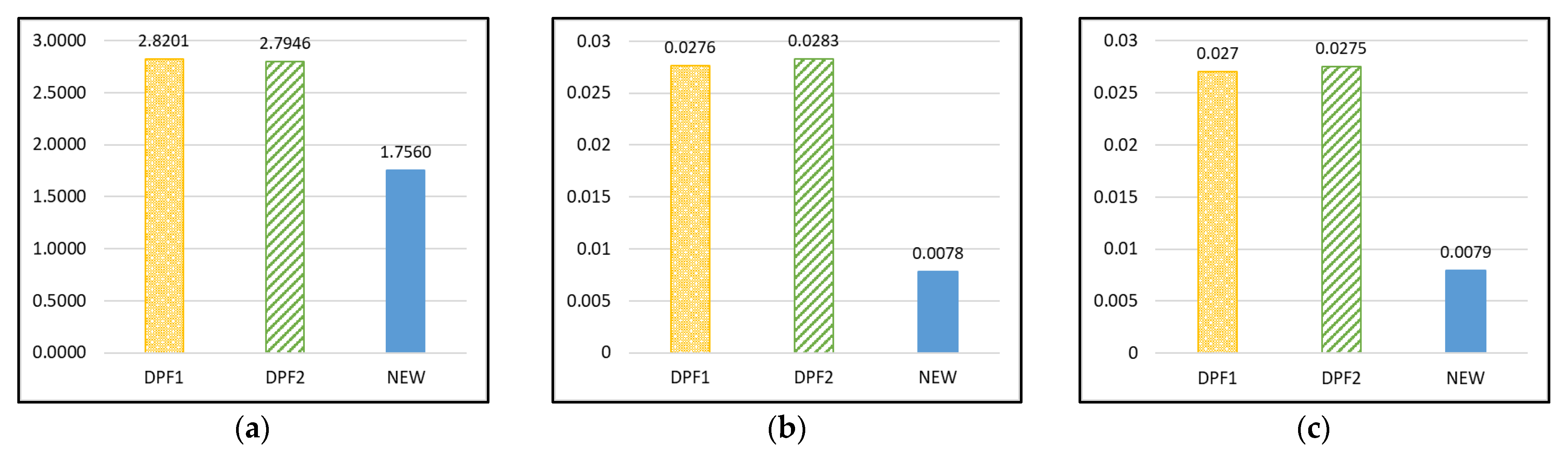
DPF1	2.8201	0.0276	0.0270	12.7389	0.9919	58.6958	60.6354	1.4321	1.4321	1.5924
DPF2	2.7946	0.0283	0.0275	12.7515	0.9919	58.6274	60.5670	1.4256	1.4256	1.5939
NEW	1.7560	0.0078	0.0079	9.0969	0.9956	57.1869	59.6115	1.0571	1.0571	1.2996

and

Table 8. Comparison of the criteria values of the models for Dataset 2.

Model	MSE	PRR	PP	SAE	R2	AIC	PRV	RMSPE	MAE	MEOP
GO	33.8121	0.4650	0.2567	119.2816	0.9658	122.0078	124.4456	5.6246	5.6897	5.1862
DS	134.5741	12.6273	1.1757	239.4995	0.8641	210.6486	213.0863	11.1425	11.3479	10.4130
IS	35.3621	0.4784	0.2614	118.4177	0.9658	123.8758	127.5324	5.6203	5.6905	5.3826
PNZ	9.8972	0.0324	0.0293	60.7847	0.9909	118.4497	123.3252	2.9414	2.9427	2.8945
PZ	38.8875	0.4653	0.2567	119.2828	0.9658	128.0082	134.1026	5.6246	5.6899	5.9641
TC	7.6738	0.0200	0.0201	47.3312	0.9933	116.9172	123.0116	2.5288	2.5288	2.3666
VTUB	7.7044	0.0223	0.0226	47.6464	0.9932	116.8753	122.9696	2.5337	2.5338	2.3823
DPF1	27.9981	0.1921	0.3654	86.1298	0.9742	141.7791	146.6546	4.9481	4.9495	4.1014
DPF2	29.5188	0.2080	0.3988	84.9504	0.9728	143.8089	148.6844	5.0737	5.0819	4.0453
NEW	7.2890	0.0163	0.0161	45.6681	0.9936	116.7360	122.8303	2.4646	2.4646	2.2834

present the estimated criteria values of the models for the two datasets. For Dataset 1, the proposed model shows the smallest MSE, PRR, PP, SAE, AIC, RMSPE, MAE, and MEOP at 1.7560, 0.0078, 0.0079, 9.0969, 57.1869, 1.0571, 1.0571, and 1.2996, respectively. The proposed model shows the largest R² at 0.9956 and the second smallest PRV at 59.6115. For Dataset 2, the proposed model shows the smallest MSE, PRR, PP, SAE, AIC, PRV, RMSPE, MAE, and MEOP at 7.2890, 0.0163, 0.0161, 45.6681, 116.7360, 122.8303, 2.4646, 2.4646, and 2.2834, respectively. The proposed model shows the largest R² at 0.9936. The results indicate that the proposed model performs better than the other models in predicting the cumulative number of failures in the datasets.

The MSE, PRR, and PP are particularly commonly used criteria. Figure 2 and Figure 3 show the top three models for the criteria (MSE, PRR, and PP) in Table 7 and Table 8. In Figure 2, the goodness of fit of the proposed model for Dataset 1 is better than that of the DPF1 and DPF2 models, which assume only dependent failures. Similarly, Figure 3 shows that the goodness of fit of the proposed model for Dataset 2 is better than that of the VTUB model, which assumes only uncertain operating environments. Thus, the proposed model, which considers both dependent failures and uncertain operating environments, is a reasonable approach for studying software reliability.

4.4. Results of SPRT

As the model proposed herein is the best fit for the datasets, we propose a method for measuring reliability by applying the SPRT based on the proposed model. Dataset 1 is used in this study. To test reliability, the SPRT is used on individual parameters or a set of parameters. For the proposed model, applying the SPRT to the parameters $\mathsf{\alpha }$ and β can lead to sensitivity issues and potentially skew the SPRT results. Therefore, the SPRT is applied specifically to parameters b, N, and c.

$${\mathrm{m}}_0\left(\mathrm{t}\right)={\mathrm{N}}_0{\left(1-\frac{\mathsf{\beta }}{\mathsf{\alpha }+\frac{{\mathrm{c}}_0}{{\mathrm{b}}_0}\ln \left(\frac{\mathsf{\alpha }+{\mathrm{e}}^{{\mathrm{b}}_0\mathrm{t}}}{1+\mathsf{\alpha }}\right)}\right)}^{\mathsf{\alpha }},{\mathrm{m}}_1\left(\mathrm{t}\right)={\mathrm{N}}_1{\left(1-\frac{\mathsf{\beta }}{\mathsf{\alpha }+\frac{{\mathrm{c}}_1}{{\mathrm{b}}_1}\ln \left(\frac{\mathsf{\alpha }+{\mathrm{e}}^{{\mathrm{b}}_1\mathrm{t}}}{1+\mathsf{\alpha }}\right)}\right)}^{\mathsf{\alpha }}.$$

(20)

Equation (20) shows the null and alternative hypotheses, ${\mathrm{m}}_0\left(\mathrm{t}\right)$ and ${\mathrm{m}}_1\left(\mathrm{t}\right)$, created based on the interval scale of the parameter groups. The parameters (${\mathrm{b}}_0$, $\mathsf{\alpha }$, $\mathsf{\beta }$, ${\mathrm{N}}_0$, and ${\mathrm{c}}_0$) represent ${\mathrm{m}}_0\left(\mathrm{t}\right)$, whereas ${\mathrm{m}}_1\left(\mathrm{t}\right)$ is represented by (${\mathrm{b}}_1$, $\mathsf{\alpha }$, $\mathsf{\beta }$, ${\mathrm{N}}_1$, and ${\mathrm{c}}_1$). The values of ${\mathrm{b}}_0$ and ${\mathrm{b}}_1$ are calculated as $\widehat{\mathrm{b}}-\mathsf{\delta }$ and $\widehat{\mathrm{b}}+\mathsf{\delta }$, respectively, where $\mathsf{\delta }$ is set as the percentile of the parameter value. For instance, when $\mathsf{\delta }$ is considered to be 1% of each parameter value, ${\mathrm{b}}_0$ is computed as $\widehat{\mathrm{b}}-0.01\times \widehat{\mathrm{b}}$, and ${\mathrm{b}}_1$ is calculated as $\widehat{\mathrm{b}}+0.01\times \widehat{\mathrm{b}}$. Similarly, percentile values are used to determine the interval scales (${\mathrm{N}}_0$, ${\mathrm{N}}_1$, ${\mathrm{c}}_0$, and ${\mathrm{c}}_1$) for N and c. The values ${\mathrm{m}}_0\left(\mathrm{t}\right)$ and ${\mathrm{m}}_1\left(\mathrm{t}\right)$ in Equation (20) are substituted into Equation (17) and based on whether $\mathrm{N}\left(\mathrm{t}\right)$ satisfies Equation (17), the conclusion is reached as “Continue” if it is satisfied. If $\mathrm{N}\left(\mathrm{t}\right)$ is smaller than the left term of Equation (17), then it is concluded as “Acceptance”. If $\mathrm{N}\left(\mathrm{t}\right)$ is bigger than the right term of Equation (17), it is concluded as “Rejection”.

To compare the SPRT results, various cases of $\mathsf{\delta }$ are considered in this study, and

Table 9. Estimation parameters of Dataset 1.

Parameter	$\mathsf{\delta }$ (30 Cases)
$\widehat{\mathrm{b}}=1.490$	${\mathsf{\delta }}_1$ = 1.490 × 0.01, ${\mathsf{\delta }}_2$ = 1.490 × 0.02, ${\mathsf{\delta }}_3$ = 1.490 × 0.03, …, ${\mathsf{\delta }}_{28}$ = 1.490 × 0.28, ${\mathsf{\delta }}_{29}$ = 1.490 × 0.29, ${\mathsf{\delta }}_{30}$ = 1.490 × 0.30
$\widehat{\mathrm{N}}=43.371$	${\mathsf{\delta }}_1$ = 43.371 × 0.01, ${\mathsf{\delta }}_2$ = 43.371 × 0.02, ${\mathsf{\delta }}_3$ = 43.371 × 0.03, …, ${\mathsf{\delta }}_{28}$ = 43.371 × 0.28, ${\mathsf{\delta }}_{29}$ = 43.371 × 0.29, ${\mathsf{\delta }}_{30}$ = 43.371 × 0.30
$\widehat{\mathrm{c}}=17.472$	${\mathsf{\delta }}_1$ = 17.472 × 0.01, ${\mathsf{\delta }}_2$ = 17.472 × 0.02, ${\mathsf{\delta }}_3$ = 17.472 × 0.03, …, ${\mathsf{\delta }}_{28}$ = 17.472 × 0.28, ${\mathsf{\delta }}_{29}$ = 17.472 × 0.29, ${\mathsf{\delta }}_{30}$ = 17.472 × 0.30

presents 30 cases of $\mathsf{\delta }$ values for $\mathrm{b}$, $\mathrm{N}$, and $\mathrm{c}$.

Table 10. Comparison of SPRT results for Dataset 1 (Cases 1–5).

T	Data	Case 1		Case 2		Case 3		Case 4		Case 5
		B	A	B	A	B	A	B	A	B	A
1	10	−91.6485	111.9572	−40.7429	61.0500	−23.7732	44.0777	−15.2878	35.5887	−10.1965	30.4928
2	12	−63.4548	86.9885	−25.8408	49.3760	−13.3007	36.8385	−7.0287	30.5700	−3.2636	26.8096
3	16	−37.5227	69.4399	−10.7830	42.7032	−1.8689	33.7940	2.5897	29.3425	5.2665	26.6746
4	22	−27.5646	72.2082	−2.6239	47.2618	5.6860	38.9424	9.8369	34.7784	12.3229	32.2753
5	28	−24.5062	82.1106	2.1452	55.4461	11.0220	46.5477	15.4519	42.0875	18.1005	39.4000
6	36	−23.4268	92.2987	5.5017	63.3539	15.1360	53.6925	19.9426	48.8478	22.8150	45.9266
7	40	−22.9201	101.2277	8.1138	70.1761	18.4491	59.8111	23.6054	54.6134	26.6865	51.4790
8	43	−22.6278	108.8320	10.2339	75.9518	21.1782	64.9767	26.6384	59.4733	29.9013	56.1548
9	44	−22.4486	115.3179	11.9897	80.8607	23.4592	69.3597	29.1818	63.5929	32.6019	60.1160
10	50	−22.3433	120.8964	13.4632	85.0707	25.3887	73.1133	31.3391	67.1181	34.8956	63.5040
11	51	−22.2903	125.7391	14.7136	88.7159	27.0381	76.3591	33.1879	70.1642	36.8639	66.4301
12	55	−22.2751	129.9798	15.7851	91.9001	28.4617	79.1912	34.7875	72.8201	38.5691	68.9802
		Continue		Continue		Continue		Continue		Continue

,

Table 11. Comparison of SPRT results for Dataset 1 (Cases 6–10).

T	Data	Case 6		Case 7		Case 8		Case 9		Case 10
		B	A	B	A	B	A	B	A	B	A
1	10	−6.8025	27.0931	−4.3786	24.6624	−2.5613	22.8372	−1.14839	21.41546	−0.0188	20.2760
2	12	−0.7517	24.3033	1.0442	22.5140	2.3929	21.1729	3.44359	20.13081	4.2858	19.2981
3	16	7.0530	24.8990	8.3312	23.6337	9.2920	22.6877	10.04157	21.95486	10.6435	21.3715
4	22	13.9757	30.6019	15.1516	29.4019	16.0287	28.4971	16.70621	27.78849	17.2434	27.2169
5	28	19.8563	37.5968	21.1001	36.2971	22.0223	35.3105	22.72883	34.53135	23.2831	33.8961
6	36	24.7175	43.9644	26.0635	42.5480	27.0597	41.4705	27.82083	40.61732	28.4158	39.9195
7	40	28.7271	49.3734	30.1705	47.8530	31.2385	46.6962	32.05422	45.77975	32.6915	45.0298
8	43	32.0626	53.9257	33.5915	52.3165	34.7230	51.0923	35.58749	50.12279	36.2631	49.3296
9	44	34.8675	57.7810	36.4707	56.0957	37.6575	54.8140	38.56454	53.79936	39.2739	52.9697
10	50	37.2520	61.0773	38.9198	59.3262	40.1549	57.9950	41.09925	56.94153	41.8382	56.0806
11	51	39.2999	63.9232	41.0244	62.1147	42.3019	60.7404	43.27912	59.65319	44.0442	58.7651
12	55	41.0753	66.4027	42.8500	64.5438	44.1650	63.1314	45.17131	62.01465	45.9596	61.1028
		Continue		Continue		Continue		Continue		Continue

,

Table 12. Comparison of SPRT results for Dataset 1 (Cases 11–15).

T	Data	Case 11		Case 12		Case 13		Case 14		Case 15
		B	A	B	A	B	A	B	A	B	A
1	10	0.9045	19.3416	1.6731	18.5610	2.3225	17.8985	2.8781	17.3287	3.3586	16.8329
2	12	4.9765	18.6179	5.5537	18.0521	6.0437	17.5744	6.4652	17.1661	6.8321	16.8132
3	16	11.1384	20.8971	11.5532	20.5046	11.9066	20.1753	12.2119	19.8959	12.4789	19.6564
4	22	17.6783	26.7445	18.0360	26.3461	18.3340	26.0045	18.5850	25.7072	18.7981	25.4452
5	28	23.7255	33.3645	24.0831	32.9097	24.3745	32.5130	24.6132	32.1613	24.8089	31.8448
6	36	28.8886	39.3332	29.2682	38.8293	29.5751	38.3874	29.8237	37.9933	30.0246	37.6362
7	40	33.1975	44.3994	33.6035	43.8570	33.9311	43.3811	34.1959	42.9560	34.4093	42.5704
8	43	36.7997	48.6630	37.2305	48.0897	37.5784	47.5868	37.8598	47.1377	38.0867	46.7305
9	44	39.8377	52.2728	40.2907	51.6738	40.6570	51.1487	40.9537	50.6801	41.1935	50.2556
10	50	42.4260	55.3578	42.8987	54.7370	43.2815	54.1932	43.5921	53.7084	43.8436	53.2694
11	51	44.6532	58.0200	45.1435	57.3804	45.5410	56.8205	45.8640	56.3218	46.1262	55.8706
12	55	46.5875	60.3381	47.0935	59.6822	47.5042	59.1084	47.8384	58.5976	48.1102	58.1359
		Continue		Continue		Continue		Continue		Continue

,

Table 13. Comparison of SPRT cases for Dataset 1 (Cases 16–20).

T	Data	Case 16		Case 17		Case 18		Case 19		Case 20
		B	A	B	A	B	A	B	A	B	A
1	10	3.7780	16.3971	4.1469	16.0107	4.4737	15.6653	4.7649	15.3544	5.0258	15.0727
2	12	7.1545	16.5056	7.4406	16.2352	7.6962	15.9959	7.9264	15.7829	8.1349	15.5922
3	16	12.7150	19.4497	12.9257	19.2699	13.1153	19.1127	13.2874	18.9747	13.4446	18.8529
4	22	18.9802	25.2116	19.1368	25.0014	19.2718	24.8106	19.3887	24.6360	19.4901	24.4751
5	28	24.9691	31.5563	25.0995	31.2903	25.2045	31.0426	25.2875	30.8097	25.3516	30.5891
6	36	30.1858	37.3084	30.3133	37.0037	30.4120	36.7175	30.4856	36.4460	30.5372	36.1863
7	40	34.5797	42.2158	34.7138	41.8856	34.8165	41.5748	34.8918	41.2794	34.9430	40.9961
8	43	38.2682	46.3561	38.4112	46.0076	38.5209	45.6795	38.6016	45.3676	38.6567	45.0686
9	44	41.3858	49.8655	41.5378	49.5027	41.6551	49.1613	41.7421	48.8371	41.8023	48.5264
10	50	44.0459	52.8664	44.2065	52.4919	44.3311	52.1400	44.4243	51.8059	44.4899	51.4860
11	51	46.3377	55.4568	46.5061	55.0725	46.6376	54.7117	46.7368	54.3695	46.8075	54.0421
12	55	48.3300	57.7128	48.5057	57.3202	48.6435	56.9519	48.7483	56.6029	48.8239	56.2693
		Continue		Continue		Continue		Continue		Continue

,

Table 14. Comparison of SPRT cases for Dataset 1 (Cases 21–25).

T	Data	Case 21		Case 22		Case 23		Case 24		Case 25
		B	A	B	A	B	A	B	A	B	A
1	10	5.2607	14.8159	5.4729	14.5805	5.6654	14.3638	5.8406	14.1631	6.0004	13.9767
2	12	8.3249	15.4207	8.4990	15.2658	8.6592	15.1253	8.8072	14.9975	8.9446	14.8808
3	16	13.5891	18.7453	13.7228	18.6499	13.8470	18.5651	13.9631	18.4897	14.0721	18.4226
4	22	19.5781	24.3260	19.6547	24.1871	19.7213	24.0570	19.7791	23.9346	19.8292	23.8192
5	28	25.3990	30.3786	25.4317	30.1766	25.4512	29.9817	25.4591	29.7928	25.4564	29.6089
6	36	30.5691	35.9361	30.5835	35.6935	30.5821	35.4568	30.5662	35.2248	30.5371	34.9965
7	40
$⋮$	$⋮$
12	55
		Reject		Reject		Reject		Reject		Reject

and

Table 15. Comparison of SPRT cases for Dataset 1 (Cases 26–30).

T	Data	Case 26		Case 27		Case 28		Case 29		Case 30
		B	A	B	A	B	A	B	A	B	A
1	10	6.1466	13.8027	6.2806	13.6396	6.4036	13.4863	6.5167	13.3417	6.6209	13.2047
2	12	9.0727	14.7739	9.1923	14.6758	9.3045	14.5856	9.4099	14.5023	9.5093	14.4254
3	16	14.1747	18.3628	14.2718	18.3095	14.3640	18.2621	14.4517	18.2199	14.5353	18.1823
4	22	19.8727	23.7098	19.9102	23.6060	19.9424	23.5071	19.9701	23.4128	19.9937	23.3227
5	28	25.4443	29.4293	25.4237	29.2535	25.3953	29.0810	25.3599	28.9113	25.3182	28.7442
6	36	30.4958	34.7708	30.4433	34.5472	30.3803	34.3251	30.3077	34.1038	30.2260	33.8831
7	40
$⋮$	$⋮$
12	55
		Reject		Reject		Reject		Reject		Reject

show the SPRT results for Dataset 1. The SPRT results from case 1 to case 20 are “Continue.” This indicates “after collecting data for the next time point, and test for the next time point.” From case 21 to case 30, the results are “Reject” at $\mathrm{t}=6,$ which indicates “stop data collection, and reject the reliability.” If the result is “Accept”, then this indicates “stop the data collection, and accept the reliability”. As the value of $\mathsf{\delta }$ increases, the area of acceptance and rejection increases, and as the value of $\mathsf{\delta }$ decreases, the area of “Continue” increases. Therefore, determining an appropriate level of $\mathsf{\delta }$ is important for the SPRT.

From Section 2.1, we can estimate reliability function $\mathrm{R}\left(\mathrm{x}|\mathrm{t}\right)$ of Dataset 1, where x is given as 0.1. Figure 4 shows the results. In Figure 4, it can be observed that the reliability sharply decreases until just before time point 5. This is estimated to be due to the rapid increase in the number of failures in Dataset 1, as indicated in Table 2. The SPRT results (cases 21–30) concluded the rejection of product reliability at the 6th time point, which aligns with the substantial number of failures in Dataset 1 up to the 6th time point. Although Dataset 1 in this study is tested for 12 weeks, according to the results of SPRT, it can be concluded that testing should be discontinued at the 6th week and efforts should be made to improve reliability.

5. Discussion

Most NHPP SRGMs assume that the testing environment is the same as the operating environment or that software failures occur independently. In this study, we propose a new NHPP SRGM that assumes uncertain operating environments and dependent failures. The results of numerical examples demonstrate the superiority of the proposed model over the models that consider only uncertain operating environments (VTUB) or only dependent failures (DPF 1 and DPF 2). Thus, the proposed model estimates the number of failures better than the existing NHPP SRGMs. This study also demonstrates how we can estimate software reliability using the proposed model by applying the SPRT. As the value of $\mathsf{\delta }$ increases, the “Continue” region becomes narrower, and the “Accept/Reject” regions become wider. Therefore, it is important to choose an appropriate level of $\mathsf{\delta }$, and further research on this matter is needed. Wood [43] explained that SRGMs can be used to predict the number of failures and provide software reliability to consumer. This study illustrates that the proposed model can be utilized in real environments.

6. Conclusions

This study had two objectives. First, we proposed a model that considered both dependent failures and uncertain operating environments. The results of the numerical examples demonstrated that the proposed model exhibited a significantly better fit than the models that considered only dependent failures (DPF 1 and DPF 2) or uncertain operating environments (VTUB).

Second, by leveraging the proposed model, we introduced a method for assessing software reliability through the application of the SPRT. Specifically, although the dataset was actually tested for 12 weeks, according to the results of the SPRT, testing was discontinued at the 6th week, and it was concluded that measures should be taken to improve the reliability. From the dataset and the values of the reliability function, it was observed that the number of failures in the observed dataset until a certain time point was higher than the number of failures after that point. In other words, even with a limited dataset, this study achieved the goal of an early reliability assessment by applying the SPRT. Further studies that link the SPRT with future software release policies will contribute to efficient development planning processes.

References

- Huang, Y.-S.; Chiu, K.-C.; Chen, W.-M. A software reliability growth model for imperfect debugging. J. Syst. Softw. 2022, 188, 111267. [Google Scholar] [CrossRef]
- Luo, H.; Xu, L.; He, L.; Jiang, L.; Long, T. A Novel Software Reliability Growth Model Based on Generalized Imperfect Debugging NHPP Framework. IEEE Access 2023, 11, 71573–71593. [Google Scholar] [CrossRef]
- Chiu, K.C.; Huang, Y.S.; Huang, I.C. A study of software reliability growth with imperfect debugging for time-dependent potential errors. Int. J. Ind. Eng.-Theory Appl. Pract. 2019, 26. [Google Scholar] [CrossRef]
- Gupta, R.; Jain, M.; Jain, A. Software Reliability Growth Model in Distributed Environment Subject to Debugging Time Lag; Springer: Berlin/Heidelberg, Germany, 2019; pp. 105–118. [Google Scholar] [CrossRef]
- Zhang, C.; Yuan, Y.; Jiang, W.; Sun, Z.; Ding, Y.; Fan, M.; Li, W.; Wen, Y.; Song, W.; Liu, K. Software Reliability Model Related to Total Number of Faults under Imperfect Debugging; Springer: Berlin/Heidelberg, Germany, 2022; pp. 48–60. [Google Scholar] [CrossRef]
- Nguyen, H.C.; Huynh, Q.T. New non-homogeneous Poisson process software reliability model based on a 3-parameter S-shaped function. IET Softw. 2022, 16, 214–232. [Google Scholar] [CrossRef]
- Pradhan, V.; Dhar, J.; Kumar, A.; Bhargava, A. An S-Shaped Fault Detection and Correction SRGM Subject to Gamma-Distributed Random Field Environment and Release Time Optimization; Springer: Berlin/Heidelberg, Germany, 2020; pp. 285–300. [Google Scholar]
- Pradhan, S.K.; Kumar, A.; Kumar, V. A Testing Coverage Based SRGM Subject to the Uncertainty of the Operating Environment. In Proceedings of the 1st International Online Conference on Mathematics and Applications, online, 1–15 May 2023; MDPI: Basel, Switzerland, 2023; p. 44. [Google Scholar]
- Pradhan, S.K.; Kumar, A.; Kumar, V. A New Software Reliability Growth Model with Testing Coverage and Uncertainty of Operating Environment. Comput. Sci. Math. Forum. 2023, 7, 44. [Google Scholar] [CrossRef]
- Pradhan, V.; Dhar, J.; Kumar, A. Testing coverage-based software reliability growth model considering uncertainty of operating environment. Syst. Eng. 2023, 26, 449–462. [Google Scholar] [CrossRef]
- Haque, M.A.; Ahmad, N. Software reliability modeling under an uncertain testing environment. Int. J. Model. Simul. 2023, 1–7. [Google Scholar] [CrossRef]
- Chatterjee, S.; Saha, D.; Sharma, A.; Verma, Y. Reliability and optimal release time analysis for multi up-gradation software with imperfect debugging and varied testing coverage under the effect of random field environments. Ann. Oper. Res. 2022, 312, 65–85. [Google Scholar] [CrossRef]
- Lee, D.H.; Chang, I.H.; Pham, H. Software Reliability Model with Dependent Failures and SPRT. Mathematics 2020, 8, 1366. [Google Scholar] [CrossRef]
- Kim, Y.S.; Song, K.Y.; Pham, H.; Chang, I.H. A Software Reliability Model with Dependent Failure and Optimal Release Time. Symmetry 2022, 14, 343. [Google Scholar] [CrossRef]
- Raheem, A.R.; Akthar, S.; Rafi, S.M. An Imperfect Debugging Software Reliability Growth Model: Optimal Release Problems through Warranty Period based on Software Maintenance Cost Model. Rev. Geintec 2021, 11, 4623–4631. [Google Scholar] [CrossRef]
- Minamino, Y.; Inoue, S.; Yamada, S. Change-point–based software reliability modeling and its application for software development management. In Recent Advancements in Software Reliability Assurance; CRC Press: Boca Raton, FL, USA, 2019; pp. 59–92. [Google Scholar]
- Ke, S.Z.; Huang, C.Y. Software reliability prediction and management: A multiple change-point model approach. Qual. Reliab. Eng. Int. 2020, 36, 1678–1707. [Google Scholar] [CrossRef]
- Saxena, P.; Kumar, V.; Ram, M. A novel CRITIC-TOPSIS approach for optimal selection of software reliability growth model (SRGM). Qual. Reliab. Eng. Int. 2022, 38, 2501–2520. [Google Scholar] [CrossRef]
- Kumar, V.; Saxena, P.; Garg, H. Selection of optimal software reliability growth models using an integrated entropy–Technique for Order Preference by Similarity to an Ideal Solution (TOPSIS) approach. In Mathematical Methods in the Applied Sciences; Wiley: Hoboken, NJ, USA, 2021. [Google Scholar] [CrossRef]
- Garg, R.; Raheja, S.; Garg, R.K. Decision Support System for Optimal Selection of Software Reliability Growth Models Using a Hybrid Approach. IEEE Trans. Reliab. 2022, 71, 149–161. [Google Scholar] [CrossRef]
- Yaghoobi, T. Selection of optimal software reliability growth model using a diversity index. Soft Comput. 2021, 25, 5339–5353. [Google Scholar] [CrossRef]
- Zhu, M. A new framework of complex system reliability with imperfect maintenance policy. Ann. Oper. Res. 2022, 312, 553–579. [Google Scholar] [CrossRef]
- Wang, J.; Zhang, C. Software reliability prediction using a deep learning model based on the RNN encoder–decoder. Reliab. Eng. Syst. Saf. 2018, 170, 73–82. [Google Scholar] [CrossRef]
- San, K.K.; Washizaki, H.; Fukazawa, Y.; Honda, K.; Taga, M.; Matsuzaki, A. Deep Cross-Project Software Reliability Growth Model Using Project Similarity-Based Clustering. Mathematics 2021, 9, 2945. [Google Scholar] [CrossRef]
- Li, L. Software reliability growth fault correction model based on machine learning and neural network algorithm. Microprocess. Microsyst. 2021, 80, 103538. [Google Scholar] [CrossRef]
- Banga, M.; Bansal, A.; Singh, A. Implementation of machine learning techniques in software reliability: A framework. In Proceedings of the 2019 International Conference on Automation, Computational and Technology Management (ICACTM), London, UK, 24–26 April 2019; IEEE: New York, NY, USA, 2019; pp. 241–245. [Google Scholar] [CrossRef]
- Wald, A. Sequential Analysis; Dover Publications: Mineola, NY, USA, 2004; ISBN 978-0-486-61579-0. [Google Scholar]
- Stieber, H.A. Statistical quality control: How to detect unreliable software components. In Proceedings of the Eighth International Symposium on Software Reliability Engineering, Albuquerque, NM, USA, 2–5 November 1997; IEEE Computer Society: Washington, DC, USA, 1997; pp. 8–12. [Google Scholar]
- Pham, H. System Software Reliability; Springer: London, UK, 2006. [Google Scholar]
- Pham, H.; Nordmann, L.; Zhang, X. A general imperfect-software-debugging model with S-shaped fault-detection rate. IEEE Trans. Reliab. 1999, 48, 169–175. [Google Scholar] [CrossRef]
- Pham, H. A new software reliability model with Vtub-shaped fault-detection rate and the uncertainty of operating environments. Optimization 2014, 63, 1481–1490. [Google Scholar] [CrossRef]
- Yamada, S.; Ohba, M.; Osaki, S. S-shaped reliability growth modeling for software fault detection. IEEE Trans. Reliab. 1983, 32, 475–484. [Google Scholar] [CrossRef]
- Goel, A.L.; Okumoto, K. Time-Dependent Error-Detection Rate Model for Software Reliability and Other Performance Measures. IEEE Trans. Reliab. 1979, 28, 206–211. [Google Scholar] [CrossRef]
- Yamada, S.; Ohba, M.; Osaki, S. S-shaped Software Reliability Growth Models and Their Applications. IEEE Trans. Reliab. 1984, 33, 289–292. [Google Scholar] [CrossRef]
- Yamada, S.; Tokuno, K.; Osaki, S. Imperfect debugging models with fault introduction rate for software reliability assessment. Int. J. Syst. Sci. 1992, 23, 2241–2252. [Google Scholar] [CrossRef]
- Pham, H.; Zhang, X. An NHPP Software Reliability Model and Its Comparison. Int. J. Reliab. Qual. Saf. Eng. 1997, 04, 269–282. [Google Scholar] [CrossRef]
- Chang, I.H.; Pham, H.; Lee, S.W.; Song, K.Y. A testing-coverage software reliability model with the uncertainty of operating environments. Int. J. Syst. Sci. Oper. Logist. 2014, 1, 220–227. [Google Scholar] [CrossRef]
- Song, K.Y.; Chang, I.H.; Pham, H. A software reliability model with a Weibull fault detection rate function subject to operating environments. Appl. Sci. 2017, 7, 983. [Google Scholar] [CrossRef]
- Li, Q.; Pham, H. A testing-coverage software reliability model considering fault removal efficiency and error generation. PLoS ONE 2017, 12, e0181524. [Google Scholar] [CrossRef]
- Akaike, H. A new look at the statistical model identification. IEEE Trans. Automat. Contr. 1974, 19, 716–723. [Google Scholar] [CrossRef]
- Pillai, K.; Sukumaran Nair, V.S. A model for software development effort and cost estimation. IEEE Trans. Softw. Eng. 1997, 23, 485–497. [Google Scholar] [CrossRef]
- Anjum, M.; Haque, M.A.; Ahmad, N. Analysis and ranking of software reliability models based on weighted criteria value. Int. J. Inf. Technol. Comput. Sci. 2013, 5, 1–14. [Google Scholar] [CrossRef]
- Wood, A. Software Reliability Growth Models; TANDEM Technical Report; Tandem Computers: Cupertino, CA, USA, 1996; Volume 96. [Google Scholar]