Numerical Investigation of a Combustible Polymer in a Rectangular Stockpile: A Spectral Approach

Abstract

Despite the wide application of combustion in reactive materials, one of the challenges faced globally is the auto-ignition of such materials, resulting in fire and explosion hazards. To avoid this unfortunate occurrence, a mathematical model describing the thermal decomposition of combustible polymer material in a rectangular stockpile is formulated. A nonlinear momentum equation is provided with the assumption that the combustible polymer follows a Carreau constitutive relation. The chemical reaction of the polymer material is assumed to be exothermic; therefore, Arrhenius’s kinetic theory is considered in the energy balance equation. The bivariate spectral local linearization scheme (BSLLS) is utilized to provide a numerical solution for the dimensionless equations governing the problem. The obtained results are validated by the collocation weighted residual method (CWRM), and a good agreement is achieved. Dimensionless velocity, temperature, and thermal stability results are presented and explained comprehensively with suitable applications. Some of the obtained results show that thermal criticality increases with increasing power law index $(n)$ and radiation $(Ra)$ values and decreases with increasing variable viscosity (${\beta }_1$) and material parameter ($W_e$) values.

1. Introduction

In engineering and industries, burning combustible materials in a slab is important for storing cellulosic materials, solid combustion, refuse cremation, heavy oil recovery, and other processes [1,2,3]. Polymers can undergo combustion and release a large amount of energy, which can then be used for transportation, generating electric power, and providing heat for various domestic and industrial applications. Compared with other energy sources, like solar cells, wind generators, and turbines, polymers are quite inexpensive. However, there are some challenges with polymer burning, such as fire ignitions due to human negligence and the physical characteristics of hydrocarbon polymers. These have caused extensive property destruction and claimed the lives of an unknown number of people. From this perspective, several authors have been prompted to study the causes of fire ignition in the combustion process and how it can be controlled.

Drysdale [4] described ignition as the process of initiating a fast exothermic reaction, which then propagates and causes changes in the materials involved and as well generates temperatures in excess. Also, ref. [4] distinguished between two kinds of ignition: (1) piloted ignition, in which a flammable mixture is ignited by a pilot such as an electrical spark or an autonomous flame, and (2) auto-ignition, in which flame develops spontaneously within the mixture. Shi and Chew [5] studied polymers’ responses to fire under auto-ignition conditions within a cone-shaped calorimeter and concluded that the $CO$ and $C{O}_2$ production process for polymers is a two-step reaction. In the first-step reaction, $CO$ and other flammable substances are generated following Arrhenius’s law. The second stage is the oxidation reaction of $CO$ in the presence of air. The whole process is expressed as follows:

$$\left\{\begin{array}{l}Step1:Polymer+O_2\to H_{2}O+CO+others product\\ Step2:CO+0.5O_2\to C{O}_2.\end{array}\right.$$

It was also discovered in [5] that the $CO$ and $C{O}_2$ emissions from flaming combustion are greater than those from non-flaming combustion.

Moreover, the combustion of polyethylene and polyvinyl chloride was examined in [6,7,8]. These investigations used experimental settings, allowing researchers to acquire more information and factors for pyrolysis, ignition, and combustion. Geschwindner et al. [9] incorporated a mix of high-speed planar laser-induced fluorescence of the HO radical (OH-PLIF) and a thermal decomposition analysis to examine the combustion of micrometer-sized polypropylene (PP) particles. They found that the highest density of flame-retardant polymer particles decreases during ignition and the early stage of burning. Lohrer et al. [10,11] investigated the effects of physical factors such as material wetness, atmospheric humidity, and concentrations of oxygen on the combustion of reactive materials and discovered that water in the reactive material increases auto-ignition.

Some mathematical models that are less expensive and faster than experimental approaches have been implemented in the literature to explain the auto-ignition of combustible materials in a stockpile. For instance, a one-step combustion process of heat transfer in a spherical channel was investigated in [12,13]. According to their reports, the system maintains stability as heat escapes into the atmosphere. In addition, enhancement in the chemical reaction rate leads to increased heat generation in the stockpile, resulting in quick auto-ignition. Lebelo et al. [14,15,16] examined the two-step thermal decomposition of combustible materials in a sphere. They identified that elevation in the two-step kinetic parameter diminishes the rate of heat loss on the sphere’s surface, which, in turn, speeds up auto-ignition.

In the literature above reviewed, the authors did not consider flow behavior in their studies. However, an increase or decrease in flow speed contributes to the heat transfer performance of combustible materials. It was discovered in the literature that the Carreau fluid model well describes the flow behavior of polymeric solutions because of its shear rate properties [17]. Several studies on Carreau fluid constitutive relations have been documented. For instance, Siska et al. [18] examined the terminal velocity of non-spherical particles falling through a Carreau fluid and concluded that the Carreau fluid model can well characterize the rheology of various polymeric solutions, such as 1% methylcellulose tylose in glycerol solutions and 3% hydroxyethyl–cellulose Natrosol HHX in glycerol solutions. Ref. [19] reported an intriguing study on the entropy production of Carreau fluid in the presence of infinite shear rate viscosity. Also, the behavior of a Carreau fluid flow past a stretching sheet was extensively analyzed in [20,21]. In addition, the peristaltic movement of a Carreau fluid was also extensively studied in [22,23,24]. For more on the Carreau fluid model with different configurations, see [25,26,27].

Motivated by the reviewed literature in [12,13,14,22,28], this study focuses on an investigation of the thermal decomposition of Carreau fluid in a rectangular stockpile with variable thermophysical properties. It is believed that this present study has not been reported in the literature. However, the outcome of this study could be useful for engineers dealing with the combustion of polymers by determining the conditions necessary for explosions and how to control them. The rest of the article is structured as follows: a mathematical model for the unsteady, fully developed flow and temperature of the polymer is presented in Section 2; Section 3 deals with the application of BSLLM to the dimensionless initial-boundary value problem; in Section 4, an extensive discussion of the obtained findings is provided; and concluding remarks are provided in Section 5.

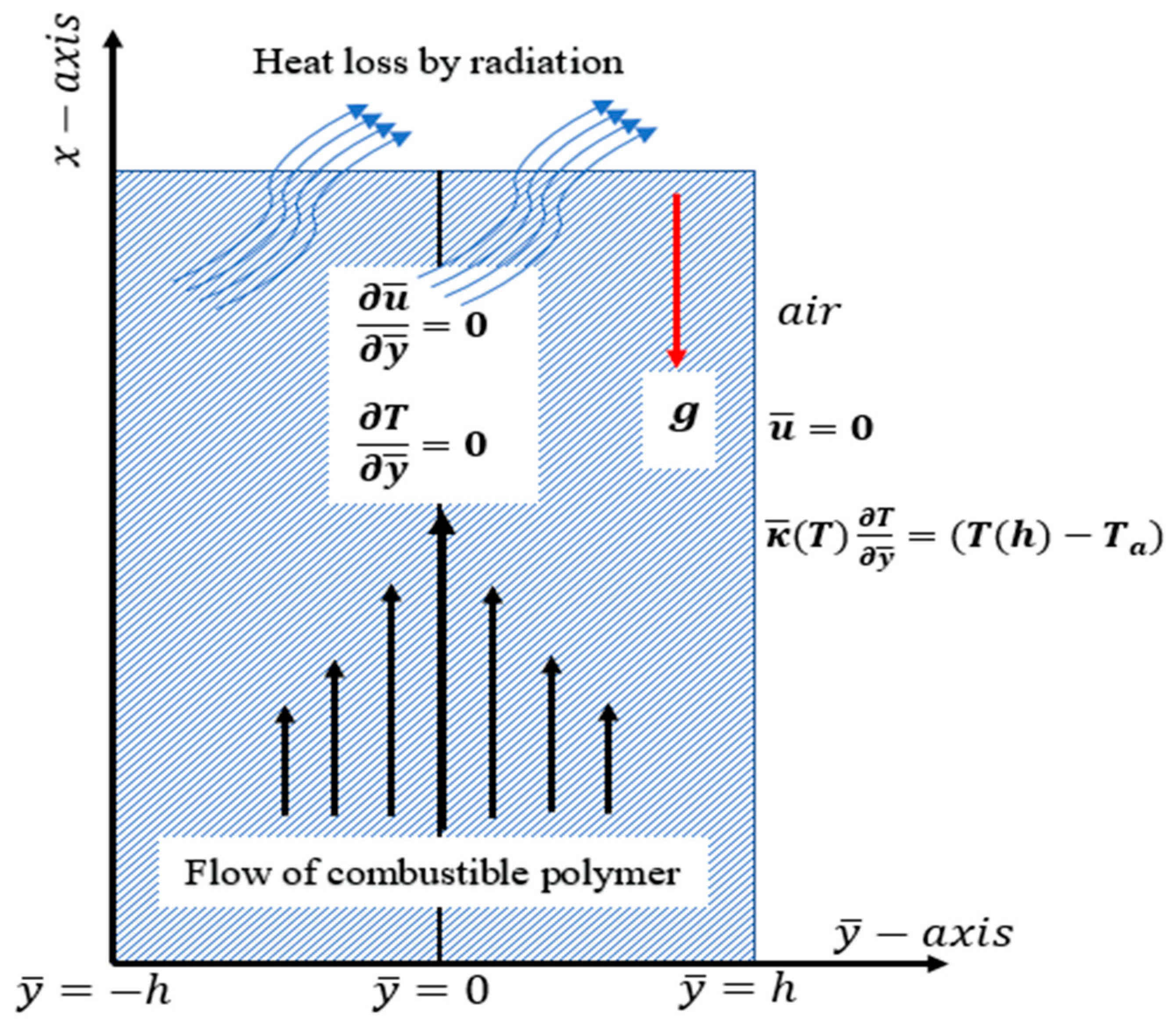
2. Mathematical Analysis

A transient laminar flow of a reactive incompressible Carreau fluid material in a combustible stockpile positioned at a distance of $2h$ apart is considered (see Figure 1). $\hat{x}-axis$ is parallel to the flow direction, and $\hat{y}-axis$ traversed to it. Initially, the fluid is assumed to be fully developed in the stockpile of the temperature, $T_0$, and the material’s viscosity and thermal conductivity, denoted as $\mu ={\mu }_0$ and $\kappa ={\kappa }_0$, respectively, are assumed to be constant. At time $\hat{t}>0$, the combustion process begins, and the material properties become temperature-dependent: $\mu =\mu (\mathrm{T})$ and $\kappa =\kappa (\mathrm{T})$. The chemistry involved in this problem assumes two-step Arrhenius kinetics. The reactant consumption is assumed negligible in this model. We also assume that the means of heat loss into the environment of the temperature, $T_a$, is mainly via radiation and convection. The influence of density variation with temperature is approximated following Boussinesque approximation. The equations governing the momentum and energy balance under the assumptions above are as follows [14,15,16,20,26]:

$$\rho \frac{\partial \hat{u}}{\partial \hat{t}}=-\frac{\partial \hat{P}}{\partial \hat{x}}+\frac{\partial }{\partial \hat{y}}\left(\mu (\mathrm{T}){\left(1+{\Gamma }^2{\left(\frac{\partial \hat{u}}{\partial \hat{y}}\right)}^2\right)}^{\frac{n-1}{2}}\frac{\partial \hat{u}}{\partial \hat{y}}\right)+\rho g\beta \left(T-T_0\right),$$

(1)

$$\begin{array}{l}\rho c_p\frac{\partial T}{\partial \hat{t}}=\frac{\partial }{\partial \hat{y}}\left(\kappa (\mathrm{T})\frac{\partial T}{\partial \hat{y}}\right)+\mu (\mathrm{T})\left({\left(1+{\Gamma }^2{\left(\frac{\partial \hat{u}}{\partial \hat{y}}\right)}^2\right)}^{\frac{n-1}{2}}{\left(\frac{\partial \hat{u}}{\partial \hat{y}}\right)}^2\right)+\\ \hspace{1em}{Q}_1{A}_1{C}_1{e}^{-\frac{E_1}{RT}}+Q_2{A}_2{C}_2{e}^{-\frac{E_2}{RT}}-\epsilon \sigma \left(T^4-T_0^4\right),\end{array}$$

(2)

with the initial-boundary conditions

$$\left.\begin{array}{l}\hat{u}\left(\hat{y},0\right)=0,T\left(\hat{y},0\right)=T_0\\ \frac{\partial \hat{u}}{\partial \hat{y}}\left(0,\hat{t}\right)=0, \frac{\partial T}{\partial \hat{y}}\left(0,\hat{t}\right)=0, \mathrm{for} \hat{t}>0\\ \hat{u}\left(\mathrm{h},\hat{t}\right)=0, -\kappa (T)\frac{\partial T}{\partial \hat{y}}(h,\hat{t})=h_t[T(h,\hat{t})-T_a], \mathrm{for} \hat{t}>0\end{array}\right\}$$

(3)

$\hat{u}—$axial velocity, $\hat{P}—$modified pressure, $T—$absolute temperature, $T_a—$ambient temperature, $T_0—$initial temperature of the stockpile, ${\mu }_0—$material’s dynamic viscosity at temperature $T_0$, ${\kappa }_0—$material’s thermal conductivity at $T_0$, $c_p—$specific heat at constant pressure, $\rho —$material’s density, $Q_1,Q_2—$first- and second-step heat of reaction, $A_1,A_2—$first- and second-step rate constants, $C_1,C_2—$first- and second-step reactant’s concentration, $E_1, E_2—$first and second step activation energies, $\epsilon —$stockpile’s emissivity $\left(0<\epsilon <1\right)$, $\sigma —$Stefan–Boltzmann constant, $\beta —$volumetric coefficient, $g—$gravitational acceleration, $h_t—$coefficient of heat transfer, $\Gamma —$time constant, $n—$dimensionless power law index. $n<1$ represents shear-thinning fluids, $n=0$ represents Newtonian fluids, and $n>1$ represents shear-thickening fluids The variable viscosity and thermal conductivity, $\overline{\mu }(\mathrm{T})$ and $\overline{\kappa }(\mathrm{T})$, are expressed, respectively, as

$$\overline{\mu }(\mathrm{T})={\mu }_0{e}^{-b_1(\mathrm{T}-{\mathrm{T}}_0)} \mathrm{and} \overline{\kappa }(\mathrm{T})={\kappa }_0{e}^{-b_2(\mathrm{T}-{\mathrm{T}}_0)},$$

(4)

where $b_1$ and $b_2$ are dynamic viscosity and thermal conductivity variation parameters. We then introduce the below dimensionless parameters to Equations (1)–(3):

$$\begin{array}{l}y=\frac{\overline{y}}{h},\mathrm{x}=\frac{\overline{x}}{h},t=\frac{\nu \overline{t}}{h^2},u=\frac{\overline{u}h}{\nu },\mu =\frac{\overline{\mu }}{{\mu }_0},\kappa =\frac{\overline{\kappa }}{{\kappa }_0},\nu =\frac{{\mu }_0}{\rho },P=\frac{\overline{P}{h}^2}{{\nu }^2},\theta =\frac{E_1\left(T-T_0\right)}{R{T}_0^2},{\theta }_a=\frac{E_1\left(T_a-T_0\right)}{R{T}_0^2}\\ ,{\beta }_1=\frac{b_{1}R{T}_0^2}{E_1},{\beta }_2=\frac{b_{2}R{T}_0^2}{E_1},W_e=\frac{\Gamma \nu }{h^2},\mathrm{Pr}=\frac{{\mu }_0{c}_p}{{\kappa }_0},\lambda =\frac{Q_1{E}_1{A}_1{h}^2{C}_1{e}^{-\frac{E_1}{R{T}_0}}}{T_0^{2}R{\kappa }_0},A=-\frac{\partial \hat{P}}{\partial \overline{x}},Gr=\frac{g\beta R{T}_0^2{h}^3{\rho }^2}{E_1{\mu }_0^2}\\ {ϵ}_1=\frac{R{T}_0}{E_1},{ϵ}_2=\frac{E_2}{E_1},V_d=\frac{{\mu }_0^3{e}^{\frac{E_1}{R{T}_0}}}{{\rho }^2{Q}_1{A}_1{h}^4{C}_1},Ra=\frac{\epsilon \sigma h^2{E}_1{T}_0^2}{R{\kappa }_0},\omega =\frac{Q_2{A}_2{E}_2}{Q_1{A}_1{E}_1}{e}^{\frac{\left(E_1-E_2\right)}{R{T}_0}},Bi=\frac{h{h}_t}{{\kappa }_0}.\\ \end{array}$$

(5)

The following dimensionless equations are then obtained:

$$\frac{\partial u}{\partial t}=A+\frac{\partial }{\partial y}\left(e^{-{\beta }_1\theta }{\left(1+W_e^2{\left(\frac{\partial u}{\partial y}\right)}^2\right)}^{\frac{n-1}{2}}\frac{\partial u}{\partial y}\right)+Gr\theta ,$$

(6)

$$\begin{array}{l}\mathrm{Pr}\frac{\partial \theta }{\partial t}=\frac{\partial }{\partial y}\left(e^{-{\beta }_2\theta }\frac{\partial \theta }{\partial y}\right)+\lambda \left(e^{\frac{\theta }{1+{ϵ}_1\theta }}+\omega e^{\frac{{ϵ}_2\theta }{1+{ϵ}_1\theta }}+V_d{e}^{-{\beta }_1\theta }{\left(1+W_e^2{\left(\frac{\partial u}{\partial y}\right)}^2\right)}^{\frac{n-1}{2}}{\left(\frac{\partial u}{\partial y}\right)}^2\right)\\ \hspace{1em}-Ra\left({\left({ϵ}_1\theta +1\right)}^4-1\right),\end{array}$$

(7)

$$\left.\begin{array}{l}u\left(y,0\right)=0,\hspace{1em}\theta \left(y,0\right)=0,\\ \frac{\partial u}{\partial y}\left(0,t\right)=0,\hspace{1em}\frac{\partial \theta }{\partial y}\left(0,t\right)=0, \mathrm{for} t>0\\ u\left(1,t\right)=0,\hspace{1em}\frac{\partial \theta }{\partial y}(1,t)=-Bi{e}^{{\beta }_2\theta }[\theta (1,t)-{\theta }_a], \mathrm{for} t>0\end{array}\right\},$$

(8)

where ${\beta }_1,{\beta }_2,W_e,\mathrm{Pr},\lambda ,{ϵ}_1,{ϵ}_2,\mathrm{A},\mathrm{Gr},{\mathrm{V}}_d,Ra,\omega ,Bi,{\theta }_a$ are, respectively, the variable viscosity parameter, the variable thermal conductivity parameter, the material parameter, the Prandtl number, the Frank–Kamenetskii parameter, the activation energy parameter, the activation energy ratio parameter, the pressure gradient, the Buoyancy parameter, the viscous heating parameter, the radiation parameter, the two-step exothermic reaction parameter, the Biot number, and the ambient temperature parameter. We also considered the Nusselt number, defined as follows:

$$Nu=\frac{h{E}_1{q}_w}{\kappa (\mathrm{T})R{\mathrm{T}}_0^2}=-{\left.\frac{\partial \theta }{\partial y}\right|}_{y=1}, \mathrm{where} q_w=-\kappa (\mathrm{T}){\left.\frac{\partial T}{\partial \hat{y}}\right|}_{\hat{y}=h}.$$

3. Solution Method

In this section, the BSLLS is implemented to provide a numerical solution for Equations (6)–(8), as outlined in [29,30]. For further studies on the convergence analysis of the BSLLS, see [31]. To adopt the BSLLS, the nonlinear equations, (6) and (7), and the nonlinear convective boundary conditions (8) are, respectively, represented by $F$, $\Theta$, and $Bc$.

$$F=A+\frac{\partial }{\partial y}\left(e^{-{\beta }_1\theta }{\left(1+W_e^2{\left(\frac{\partial u}{\partial y}\right)}^2\right)}^{\frac{n-1}{2}}\frac{\partial u}{\partial y}\right)+Gr\theta -\frac{\partial u}{\partial t},$$

(9)

$$\begin{array}{l}\Theta =\frac{\partial }{\partial y}\left(e^{-{\beta }_2\theta }\frac{\partial \theta }{\partial y}\right)+\lambda \left(e^{\frac{\theta }{1+{ϵ}_1\theta }}+\omega e^{\frac{{ϵ}_2\theta }{1+{ϵ}_1\theta }}+V_d{e}^{-{\beta }_1\theta }{\left(1+W_e^2{\left(\frac{\partial u}{\partial y}\right)}^2\right)}^{\frac{n-1}{2}}{\left(\frac{\partial u}{\partial y}\right)}^2\right)\\ \hspace{1em}-Ra\left({\left({ϵ}_1\theta +1\right)}^4-1\right)-\mathrm{Pr}\frac{\partial \theta }{\partial t},\end{array}$$

(10)

$$Bc=\frac{\partial \theta }{\partial y}(1,t)+Bi{e}^{{\beta }_2\theta (1,t)}[\theta (1,t)-{\theta }_a]$$

(11)

The iteration technique (quasi-linearization method) is applied independently to Equations (9)–(11) to arrive at

$$\begin{array}{l}{\alpha }_{0,r}(y,t)\frac{{\partial }^2{u}_{r+1}}{\partial y^2}+{\alpha }_{1,r}(y,t)\frac{\partial u_{r+1}}{\partial y}+{\alpha }_{2,r}(y,t)\frac{\partial u_{r+1}}{\partial t}={ℝ}_{1,r}(y,t),\\ \end{array}$$

(12)

$${\beta }_{0,r}(y,t)\frac{{\partial }^2{\theta }_{r+1}}{\partial y^2}+{\beta }_{1,r}(y,t)\frac{\partial {\theta }_{r+1}}{\partial y}+{\beta }_{2,r}(y,t){\theta }_{r+1}+{\beta }_{3,r}(y,t)\frac{\partial {\theta }_{r+1}}{\partial t}={ℝ}_{2,r}(y,t),$$

(13)

$$c_{0,r}(1,t)\frac{\partial {\theta }_{r+1}}{\partial y}+c_{1,r}(1,t){\theta }_{r+1}=d_r(1,t),$$

(14)

where

$$\begin{array}{l}{\alpha }_{0,r}(y,t)=\frac{\partial F}{\partial \left(\frac{{\partial }^{2}u}{\partial y^2}\right)}=e^{-{\beta }_1\theta }\left(1+n{W}_e^2{\left(\frac{\partial u}{\partial y}\right)}^2\right){\left(1+W_e^2{\left(\frac{\partial u}{\partial y}\right)}^2\right)}^{\frac{n-3}{2}},\\ {\alpha }_{1,r}(y,t)=\frac{\partial F}{\partial \left(\frac{\partial u}{\partial y}\right)}=e^{-{\beta }_1\theta }\left(\begin{array}{l}\left(n-1\right)W_e^2\frac{\partial u}{\partial y}\left(3+n{W}_e^2{\left(\frac{\partial u}{\partial y}\right)}^2\right)\frac{{\partial }^{2}u}{\partial y^2}-\\ {\beta }_1\left(1+W_e^2{\left(\frac{\partial u}{\partial y}\right)}^2\right)\left(1+n{W}_e^2{\left(\frac{\partial u}{\partial y}\right)}^2\right)\frac{\partial \theta }{\partial y}\end{array}\right){\left(1+W_e^2{\left(\frac{\partial u}{\partial y}\right)}^2\right)}^{\frac{n-5}{2}},\\ {\alpha }_{2,r}(y,t)=\frac{\partial F}{\partial \left(\frac{\partial u}{\partial t}\right)}=-1,{\beta }_{0,r}(y,t)=\frac{\partial T}{\partial \left(\frac{{\partial }^2\theta }{\partial y^2}\right)}=e^{-{\beta }_2\theta },{\beta }_{1,r}(y,t)=\frac{\partial T}{\partial \left(\frac{\partial \theta }{\partial y}\right)}=-2{\beta }_2{e}^{-{\beta }_2\theta }\frac{\partial \theta }{\partial y},\end{array}$$

$$\begin{array}{l}{\beta }_{2,r}(y,t)=\frac{\partial T}{\partial \theta }=\frac{\lambda \left({\beta }_2{V}_d{\left(\frac{\partial u}{\partial y}\right)}^2\left(-e^{-{\beta }_2\theta }\right){\left({ϵ}_1\theta +1\right)}^2{\left(W_e^2{\left(\frac{\partial u}{\partial y}\right)}^2+1\right)}^{\frac{n-1}{2}}+\omega {ϵ}_2{e}^{\frac{{ϵ}_2\theta }{{ϵ}_1\theta +1}}+e^{\frac{\theta }{{ϵ}_1\theta +1}}\right)}{{\left({ϵ}_1\theta +1\right)}^2}+\\ \hspace{1em}{\beta }_2^2{e}^{-{\beta }_2\theta }{\left(\frac{\partial \theta }{\partial y}\right)}^2-{\beta }_2{e}^{-{\beta }_2\theta }\frac{{\partial }^2\theta }{\partial y^2}-4\mathrm{Ra}{ϵ}_1{\left({ϵ}_1\theta +1\right)}^3,\end{array}$$

$${\beta }_{3,r}(y,t)=\frac{\partial T}{\partial \left(\frac{\partial \theta }{\partial t}\right)}=-\mathrm{Pr}, c_{0,r}(1,t)=\frac{\partial Bc}{\partial \left(\frac{\partial \theta }{\partial y}\right)}=1,$$

$$\begin{array}{l}{c}_{1,r}(1,t)=\frac{\partial Bc}{\partial \theta }={\beta }_{2}Bi{\theta }_r(1,t)+Bi{e}^{{\beta }_2{\theta }_r(1,t)}-{\beta }_{2}Bi{\theta }_a{e}^{{\beta }_2{\theta }_r(1,t)},\\ d_r(1,t)=c_{0,r}(1,t)\frac{\partial {\theta }_r}{\partial y}+c_{1,r}(1,t){\theta }_r-B{c}_r(1,t),\\ {ℝ}_{1,r}(y,t)={\alpha }_{0,r}(y,t)\frac{{\partial }^2{u}_r}{\partial y^2}+{\alpha }_{1,r}(y,t)\frac{\partial u_r}{\partial y}+{\alpha }_{2,r}(y,t)\frac{\partial u_r}{\partial t}-F_r(y,t),\\ {ℝ}_{2,r}(y,t)={\beta }_{0,r}(y,t)\frac{{\partial }^2{\theta }_r}{\partial y^2}+{\beta }_{1,r}(y,t)\frac{\partial {\theta }_r}{\partial y}+{\beta }_{2,r}(y,t){\theta }_r+{\beta }_{3,r}(y,t)\frac{\partial {\theta }_r}{\partial t}-{\Theta }_r(y,t).\end{array}$$

The next step is to transform the physical domains, $t\in [0,T]$ and $y\in [0,1]$, respectively, into domains $\tau \in [-1,1]$ and $x\in [-1,1]$ using transformations $t=\frac{T(\tau +1)}{2}$ and $y=\frac{(x+1)}{2}$,

with collocation points

$$x_i={\left\{cos(\frac{\pi i}{N_x})\right\}}_{i=0}^{N_x} \mathrm{and} {\tau }_j={\left\{cos(\frac{\pi j}{N_{\tau }})\right\}}_{j=0}^{N_{\tau }}.$$

It is assumed that solutions to $u(\tau ,x)$ and $\theta (\tau ,x)$, in the form of bivariate Lagrange’s interpolating polynomials, are defined as:

$$\begin{array}{l}u(x,\tau )\approx {\displaystyle \sum _{p=0}^{N_y}{\displaystyle \sum _{q=0}^{N_t}u\left(x_i,{\tau }_j\right)L_p(x)L_q(\tau )}},\\ \theta (x,\tau )\approx {\displaystyle \sum _{p=0}^{N_y}{\displaystyle \sum _{q=0}^{N_t}\theta \left(x_i,{\tau }_j\right)L_p(x)L_q(\tau )}},\end{array}$$

(15)

where function $L_p(x)$ represents the Lagrange cardinal polynomial of the Chebyshev–Gaus–Lobatto grid points,

$$L_p\left(x\right)={\displaystyle \prod _{\begin{array}{c}p=0\\ p\ne i\end{array}}^{N_x}\frac{x-x_i}{x_p-x_i}},$$

(16)

with $L_p(x_i)={\delta }_{ip}=\left\{\begin{array}{l}0,i\ne p\hfill \\ 1,i=p\hfill \end{array}\right.$.

The $L_q\left(\tau \right)$ function is defined similarly. The derivative values at the Chebyshev–Gaus–Lobatto points $(x_i,{\tau }_j)$ are computed as follows:

$$\begin{array}{l}\frac{{\partial }^{r}u}{\partial x^r}(x_i,{\tau }_j)=2^r{\displaystyle \sum _{p=0}^{N_x}{D}_{i,p}^{r}u(x_p,{\tau }_j)}=D^r{u}_j,\\ \frac{\partial u}{\partial \tau }(x_i,{\tau }_j)=\frac{2}{T}{\displaystyle \sum _{q=0}^{N_{\tau }}{d}_{j,q}u(x_i,{\tau }_q)={\displaystyle \sum _{q=0}^{N_{\tau }}{\hat{d}}_{j,q}{u}_q}},\\ \frac{{\partial }^r\theta }{\partial x^r}(x_i,{\tau }_j)=2^r{\displaystyle \sum _{p=0}^{N_x}{D}_{i,p}^r\theta (x_p,{\tau }_j)}=D^r{\theta }_j,\\ \frac{\partial \theta }{\partial \tau }(x_i,{\tau }_j)=\frac{2}{T}{\displaystyle \sum _{q=0}^{N_{\tau }}{d}_{j,q}\theta (x_i,{\tau }_q)}={\displaystyle \sum _{q=0}^{N_{\tau }}{\hat{d}}_{j,q}{\theta }_q},\end{array}$$

(17)

where r is the order of the derivative, and $D^r=2^r{D}_{i,p}^r$ and ${\hat{d}}_{j,q}=\frac{2}{T}{d}_{j,q}$ are Chebyshev differentiation matrices $(N_x+1)\times (N_x+1)$ and $(N_{\tau }+1)\times (N_{\tau }+1)$ respectively. $u_j$ and ${\theta }_j$ are defined as

$$\begin{array}{l}{u}_j={[u(x_0,{\tau }_j),u(x_1,{\tau }_j),u(x_2,{\tau }_j),\dots ,u(x_{N_x},{\tau }_j)]}^T, for j=0,1,2,\dots ,N_{\tau },\\ {\theta }_j={[\theta (x_0,{\tau }_j),\theta (x_1,{\tau }_j),\theta (x_2,{\tau }_j),\dots ,\theta (x_{N_x},{\tau }_j)]}^T,for j=0,1,2,\dots ,N_{\tau },\end{array}$$

(18)

Superscript T denotes a transpose. Substituting Equations (17) and (18) into (12) and (13) yields

$$\begin{array}{l}{\alpha }_{0,r}(x,{\tau }_j)D^2{u}_{r+1,j}+{\alpha }_{1,r}(x,{\tau }_j)D{u}_{r+1,j}+{\alpha }_{{}_{2,r}}(x,{\tau }_j){\displaystyle \sum _{q=0}^{N_{\tau }}{\hat{d}}_{j,q}{u}_{r+1,q}}={ℝ}_{1,r}(x,{\tau }_j),\\ {\beta }_{{}_{0,r}}(x,{\tau }_j)D^2{\theta }_{r+1,j}+{\beta }_{1,r}(x,{\tau }_j)D{\theta }_{r+1,j}+{\beta }_{2,r}(x,{\tau }_j)I+{\beta }_{3,r}(x,{\tau }_j){\displaystyle \sum _{q=0}^{N_{\tau }}{\hat{d}}_{j,q}{\theta }_{r+1,q}}={ℝ}_{2,r}(x,{\tau }_j),\end{array}$$

(19)

where

$$\begin{array}{l}{\alpha }_{k,r}(x,{\tau }_j) (k=0,1,2)=\left(\begin{array}{ccc}{\alpha }_{k,r}(x_0,{\tau }_j)& & \\ & \ddots & \\ & & {\alpha }_{k,r}(x_{N_x},{\tau }_j)\end{array}\right),\\ {\beta }_{k,r}(x,{\tau }_j) (k=0,1,2,3)=\left(\begin{array}{ccc}{\beta }_{k,r}(x_0,{\tau }_j)& & \\ & \ddots & \\ & & {\beta }_{k,r}(x_{N_x},{\tau }_j)\end{array}\right),\end{array}$$

$$\begin{array}{l}{ℝ}_{1,r}(x,{\tau }_j)={\alpha }_{0,r}(x,{\tau }_j)D^2{u}_{r,j}+{\alpha }_{1,r}(x,{\tau }_j)D{u}_{r,j}+{\alpha }_{{}_{2,r}}(x,{\tau }_j){\displaystyle \sum _{q=0}^{N_{\tau }}{\hat{d}}_{j,q}{u}_{r,q}}-F_r(x,{\tau }_j),\\ {ℝ}_{2,r}(x,{\tau }_j)={\beta }_{0,r}(x,{\tau }_j)D^2{\theta }_{r,j}+{\beta }_{1,r}(x,{\tau }_j)D{\theta }_{r,j}+{\beta }_{2,r}(x,{\tau }_j){\theta }_{r,j}+{\beta }_{3,r}(x,{\tau }_j){\displaystyle \sum _{q=0}^{N_{\tau }}{\hat{d}}_{j,q}{\theta }_{r,q}}-{\Theta }_r(x,{\tau }_j),\end{array}$$

and $I$ is an identity matrix. Applying spectral collocation to the boundary conditions (8) and the convective boundary condition (14), we have

$$\begin{array}{l}{\displaystyle \sum _{p=0}^{N_x}2D_{N_x,p}{u}_{r+1}(x_p,{\tau }_j)}=0,\hspace{1em}{u}_{r+1}\left(x_0,{\tau }_j\right)=0,\\ {\displaystyle \sum _{p=0}^{N_x}2D_{N_x,p}{\theta }_{r+1}(x_p,{\tau }_j)}=0,\hspace{1em}{c}_{0,r}(x_0,{\tau }_j){\displaystyle \sum _{p=0}^{N_x}2D_{0,p}{\theta }_{r+1}(x_p,{\tau }_j)}+c_{1,r}(x_0,{\tau }_j){\theta }_{r+1}(x_0,{\tau }_j)=d_r(x_0,{\tau }_j).\end{array}$$

Imposing boundary conditions on Equation (19) for $j=0,1,\dots ,N_{\tau }-1$, we obtain the following $N_{\tau }(N_x+1)\times N_{\tau }(N_x+1)$ system of matrices:

$$\begin{array}{l}\left[\begin{array}{cccc}{A}_{1(0,0)}& A_{1(0,1)}& \dots & A_{1(0,N_{\tau }-1)}\\ A_{1(1,0)}& A_{1(1,1)}& \dots & A_{1(1,N_{\tau }-1)}\\ ⋮& ⋮& ⋮& ⋮\\ A_{1(N_{\tau }-1,0)}& A_{1(N_{\tau }-1,1)}& \dots & A_{1(N_{\tau }-1,N_{\tau }-1)}\end{array}\right] \left[\begin{array}{c}{u}_{r+1,0}\\ u_{r+1,1}\\ ⋮\\ u_{r+1,N_{\tau }-1}\end{array}\right]=\left[\begin{array}{c}{ℝ}_1(x,0)\\ {ℝ}_1(x,1)\\ ⋮\\ {ℝ}_1(x,N_{\tau }-1)\end{array}\right],\\ \left[\begin{array}{cccc}{A}_{2(0,0)}& A_{2(0,1)}& \dots & A_{2(0,N_{\tau }-1)}\\ A_{2(1,0)}& A_{2(1,1)}& \dots & A_{2(1,N_{\tau }-1)}\\ ⋮& ⋮& ⋮& ⋮\\ A_{2(N_{\tau }-1,0)}& A_{2(N_{\tau }-1,1)}& \dots & A_{2(N_{\tau }-1,N_{\tau }-1)}\end{array}\right]\left[\begin{array}{c}{\theta }_{r+1,0}\\ {\theta }_{r+1,1}\\ ⋮\\ {\theta }_{r+1,N_{\tau }-1}\end{array}\right]=\left[\begin{array}{c}{ℝ}_2(x,0)\\ {ℝ}_2(x,1)\\ ⋮\\ {ℝ}_2(x,N_{\tau }-1)\end{array}\right],\end{array}$$

(20)

with

$$\begin{array}{l}{A}_{1(j,j)}={\alpha }_{0,r}(x,{\tau }_j)D^2+{\alpha }_{1,r}(x,{\tau }_j)D+{\alpha }_{{}_{2,r}}(x,{\tau }_j){\hat{d}}_{j,j}I=,j=0,1,\cdots ,N_{\tau }-1,\\ A_{1(j,i)}={\alpha }_{{}_{2,r}}(x,{\tau }_j){\hat{d}}_{j,i}I,when j\ne i, \\ {ℝ}_1(x,{\tau }_j)={ℝ}_{1,r}(x,{\tau }_j)-{\alpha }_{{}_{2,r}}(x,{\tau }_j){\hat{d}}_{j,N_{\tau }}{u}_{r+1,N_{\tau }},\hspace{1em}for\hspace{1em}j=0,1,\cdots ,N_{\tau }-1,\\ A_{2(j,j)}={\beta }_{{}_{0,r}}(x,{\tau }_j)D^2+{\beta }_{1,r}(x,{\tau }_j)D+{\beta }_{2,r}(x,{\tau }_j)I+{\beta }_{3,r}(x,{\tau }_j){\hat{d}}_{j,j}I,\hspace{1em}j=0,1,\cdots ,N_{\tau }-1,\\ A_{2(j,i)}={\beta }_{3,r}(x,{\tau }_j){\hat{d}}_{j,i},\hspace{1em}when\hspace{1em}j\ne i,\\ {ℝ}_2(x,{\tau }_j)={ℝ}_{2,r}(x,{\tau }_j)-{\beta }_{{}_{3,r}}(x,{\tau }_j){\hat{d}}_{j,N_{\tau }}{\theta }_{r+1,N_{\tau }},\hspace{1em}for\hspace{1em}j=0,1,\cdots ,N_{\tau }-1,\\ \end{array}$$

The vectors $u_{r+1,N_{\tau }}$ and ${\theta }_{r+1,N_{\tau }}$ correspond to the initial condition given in Equation (8). The matrices (20) are solved iteratively until suitable results are obtained.

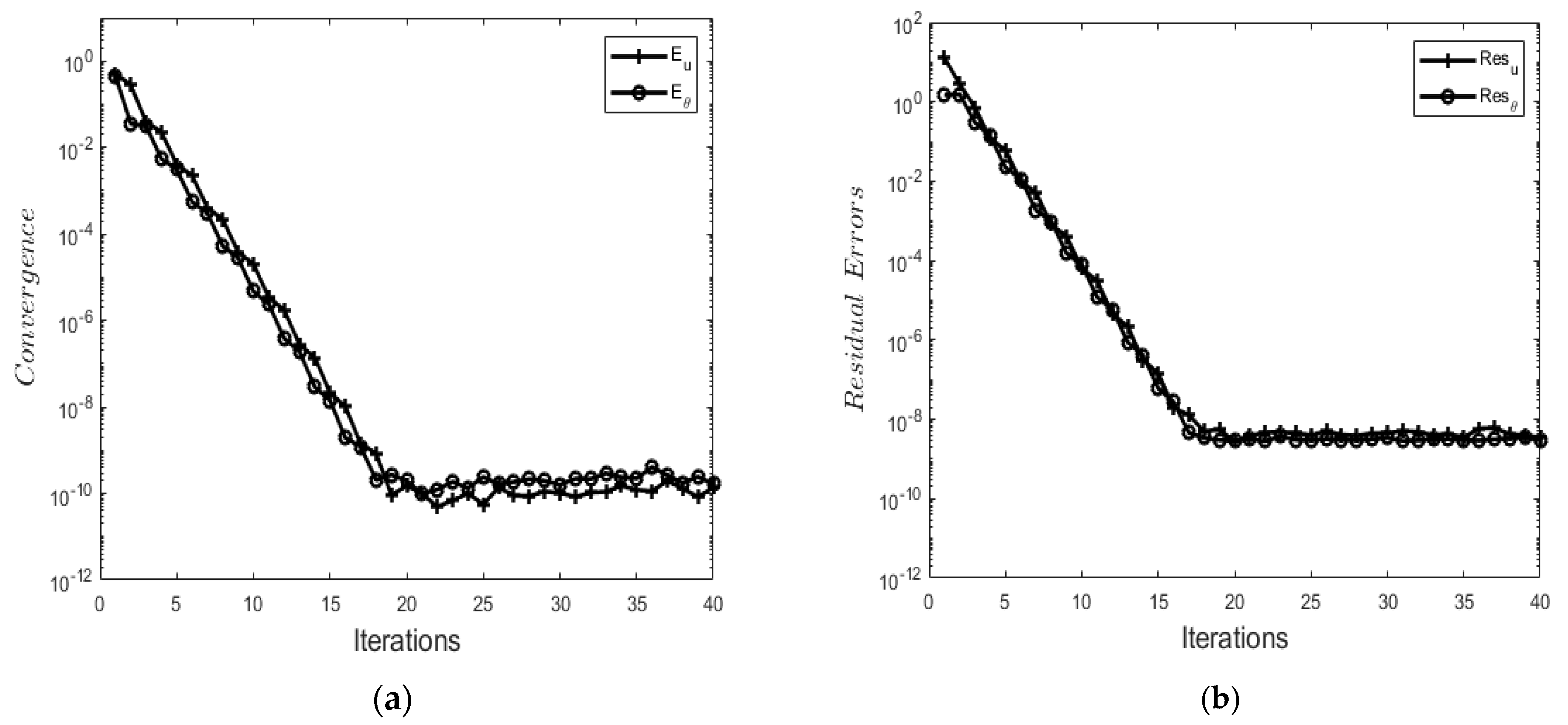
Convergence Analysis

The convergence of the BSLLS is evaluated by considering the error norms between two successive iterations. Error norms are defined as

$$\begin{array}{l}{E}_u=\underset{0<i<N_t}{{\displaystyle \max }}‖u_{r+1,i}-u_{r,i}‖,\\ E_{\theta }=\underset{0<i<N_t}{{\displaystyle \max }}‖{\theta }_{r+1,i}-{\theta }_{r,i}‖,\end{array}$$

(21)

$E_u$ and $E_{\theta }$ decrease swiftly as the number of iterations increases (see Figure 2a. This shows that the BSLLS converges within a few iterations. Also, residual error norms are computed to show the accuracy of the BSLLS. Residual error norms are expressed as

$$\begin{array}{l}{R}_u=\underset{0<i<N_t}{{\displaystyle \max }}‖{\partial }_u\left(F\right)‖,\\ R_{\theta }=\underset{0<i<N_t}{{\displaystyle \max }}‖{\partial }_{\theta }\left(\Theta \right)‖,\end{array}$$

(22)

where ${\partial }_u$ and ${\partial }_{\theta }$ are corresponding nonlinear partial differential equations: Equations (9) and (10), respectively. Figure 2b depicts residual errors $R_u$ and $R_{\theta }$ against the number of iterations. Residual errors are found to decrease rapidly with an increasing number of iterations.

4. Results and Discussion

In this section, we employ the parameter values, $n=0.5, W_e=0.5, A=1, {\beta }_1=0.1, {\beta }_2=0.1,$ $\lambda =0.1, {ϵ}_1=0.1,\hspace{1em}{ϵ}_2=0.1, \omega =1, Ra=0.1, \mathrm{Pr}=10, Gr=1, V_d=0.5,\hspace{1em}{\theta }_a=0.1, A=1,T=120,$ as default values, unless otherwise stated in graphs and tables. The results obtained by using the BSLLS are validated with the ones obtained using the collocation weighted residual method (see

Table 1. Validation of bivariate spectral local linearization method with Chebyshev collocation method.

$\mathbf{y}$	${\mathbf{u}}_{\mathit{B}\mathit{S}\mathit{L}\mathit{L}\mathit{M}}$	${\mathbf{u}}_{\mathit{C}\mathit{W}\mathit{R}\mathit{M}}$	${\mathbf{\theta }}_{\mathit{B}\mathit{S}\mathit{L}\mathit{L}\mathit{M}}$	${\mathbf{\theta }}_{\mathit{C}\mathit{W}\mathit{R}\mathit{M}}$
0.00	0.8472544166	$0.8472544291$	0.5231137461	0.5231137500
0.25	0.7969166162	$0.7969166280$	0.5149631360	$0.5149631391$
0.50	0.6436905650	$0.6436905747$	0.4901023867	$0.4901023899$
0.75	0.3812086637	$0.3812086696$	0.4472855132	$0.4472855163$
1.00	$-9.59276\times {10}^{-14}$	$-1.12618\times {10}^{-23}$	0.3843857453	$0.3843857480$

), and a good agreement is observed.

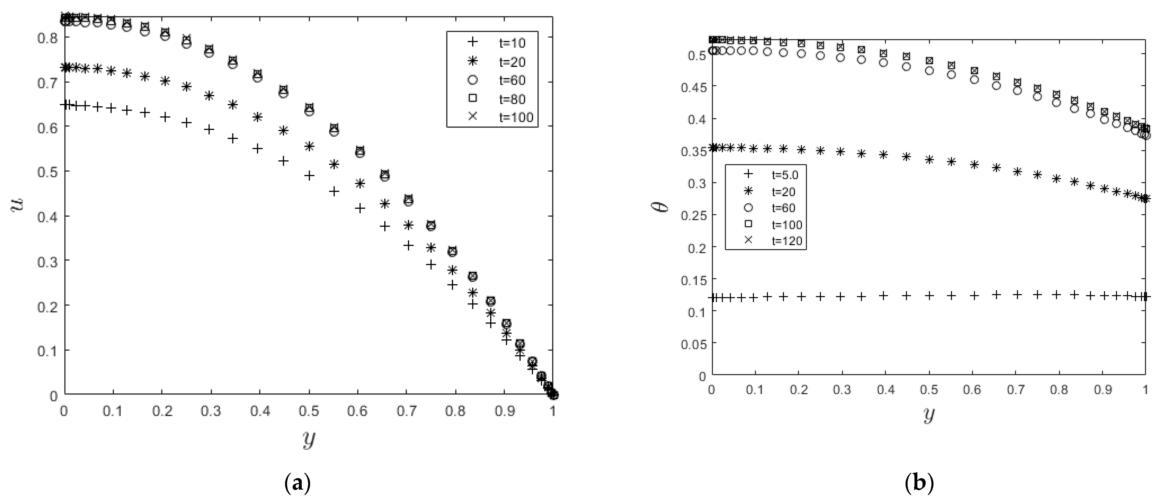
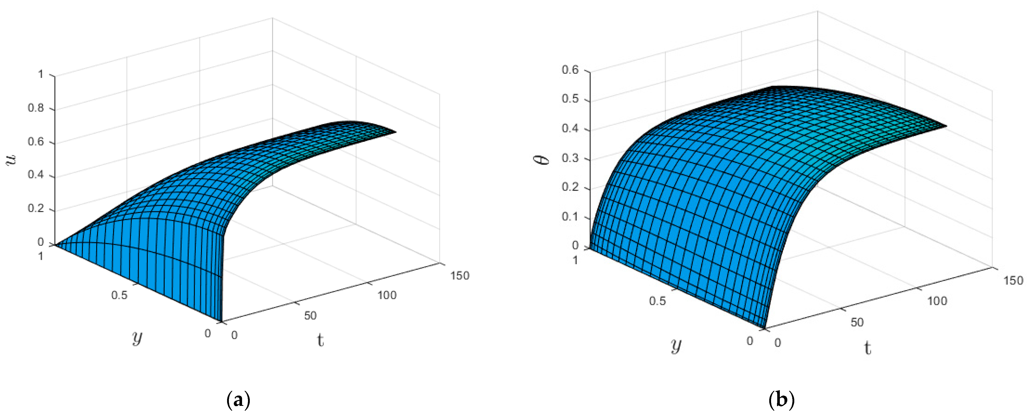
4.1. Transient Profiles for Velocity and Temperature

Figure 3 and Figure 4 show the time development of the velocity and temperature profiles. As time passes, the velocity (Figure 3a) and temperature (Figure 3b) profiles rise until they reach steady-state maximum values. Furthermore, the velocity profile reaches a steady state faster than the temperature profile. This is expected since velocity acts as a source of heat for the combustion process and, hence, increases the temperature profile.

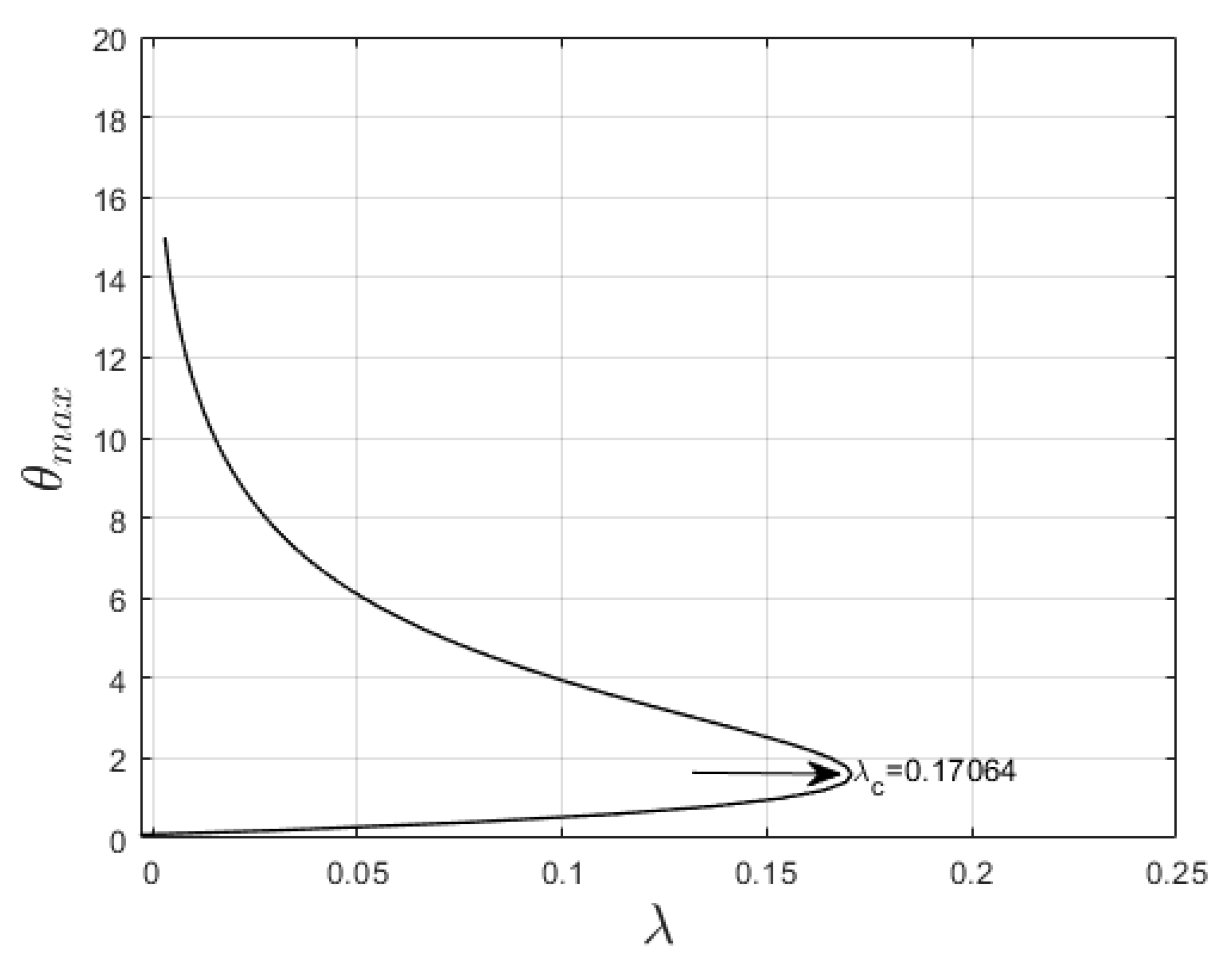
4.2. Solution Blow-Up Profile

The bifurcation plot of the maximum temperature, $(\theta (0))$, versus the Frank–Kamenetskii parameter, $\lambda$, is provided to examine the thermal criticality condition of the system. The critical value, ${\lambda }_c$, is computed at a steady state (when combustion is independent of time) to explain auto-ignition during the combustion process. Figure 5 displays a bifurcation diagram explaining the thermal behavior of the system as $\lambda$ increases. The bifurcation diagram illustrates that the solution to Equation (7), at a steady state, is finite for $\lambda$ between interval $0$ and ${\lambda }_c$. Auto-ignition is observed at the upper limit of the interval, ${\lambda }_c$, and a real solution does not exist when $\lambda >{\lambda }_c$.

To prevent or control spontaneous ignition, the impact of the thermophysical parameters on the thermal criticality is examined (see

Table 2. Variations in criticality values for $A=1, \omega =1, Gr=1, \mathrm{Pr}=10,{ϵ}_1=0.1,\hspace{1em}{ϵ}_2=0.1,\hspace{1em}{V}_d=0.5,T=120$.

${\mathbf{\beta }}_1$	${\mathbf{\beta }}_2$	${\mathbf{W}}_{\mathit{e}}$	$\mathbf{n}$	$\mathbf{R}\mathbf{a}$	$\mathbf{B}\mathbf{i}$	${\mathbf{\lambda }}_{\mathit{c}}$
0.1	0.1	0.5	0.5	0.1	1.0	0.17064
0.3	0.1	0.5	0.5	0.1	1.0	0.15603
0.5	0.1	0.5	0.5	0.1	1.0	0.14231
0.1	0.1	0.5	0.5	0.1	1.0	0.17064
0.1	0.3	0.5	0.5	0.1	1.0	0.15942
0.1	0.5	0.5	0.5	0.1	1.0	0.14860
0.1	0.1	0.1	0.5	0.1	1.0	0.18038
0.1	0.1	0.3	0.5	0.1	1.0	0.17695
0.1	0.1	0.5	0.5	0.1	1.0	0.17064
0.1	0.1	0.5	0.5	0.1	1.0	0.17064
0.1	0.1	0.5	1.0	0.1	1.0	0.18081
0.1	0.1	0.5	1.5	0.1	1.0	0.18591
0.1	0.1	0.5	0.5	0.1	1.0	0.17064
0.1	0.1	0.5	0.5	0.3	1.0	0.19447
0.1	0.1	0.5	0.5	0.5	1.0	0.21836
0.1	0.1	0.5	0.5	0.1	0.5	0.10362
0.1	0.1	0.5	0.5	0.1	1.0	0.17064
0.1	0.1	0.5	0.5	0.1	1.5	0.22120

). Thermal criticality increases with increasing values of the power law index $(n)$, radiation $(Ra)$, and the Biot number $(Bi)$ and decreases with increasing values of variable viscosity (${\beta }_1$), the variable thermal conductivity parameter (${\beta }_2$), and the material parameter ($W_e$). This implies that these factors are important in minimizing auto-ignition. In other words, for thermal stability to be maintained during combustion processes, these parameters should be made significant.

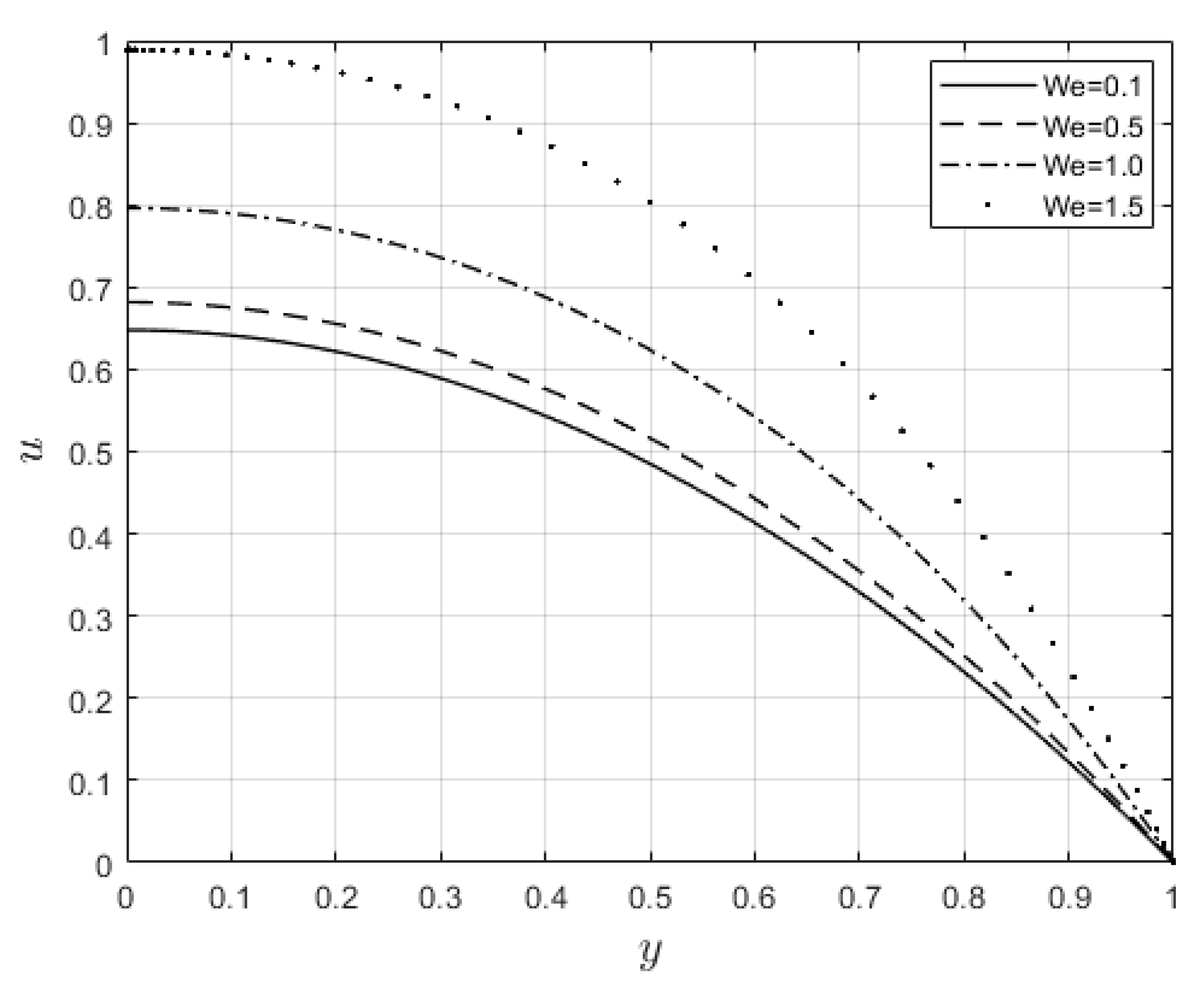
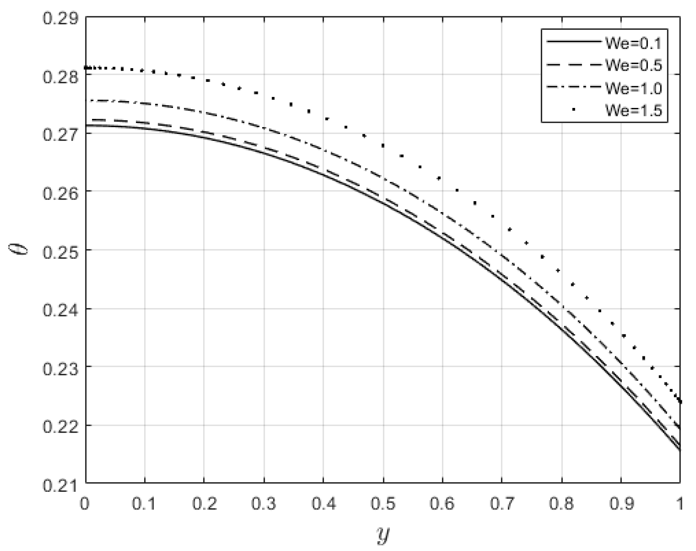
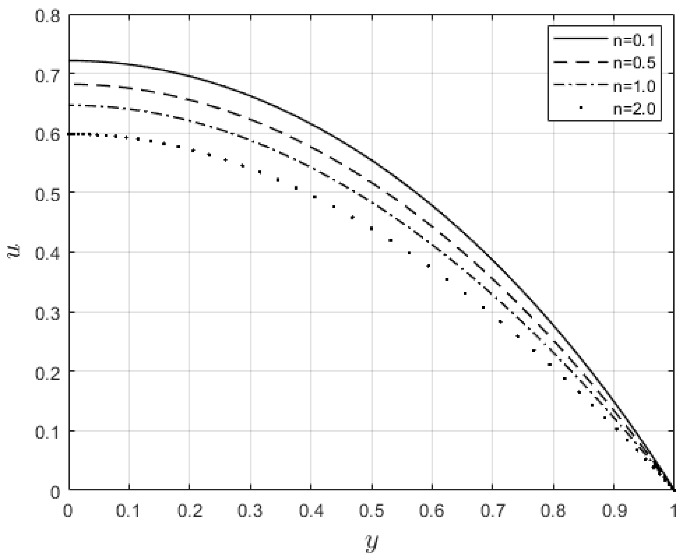
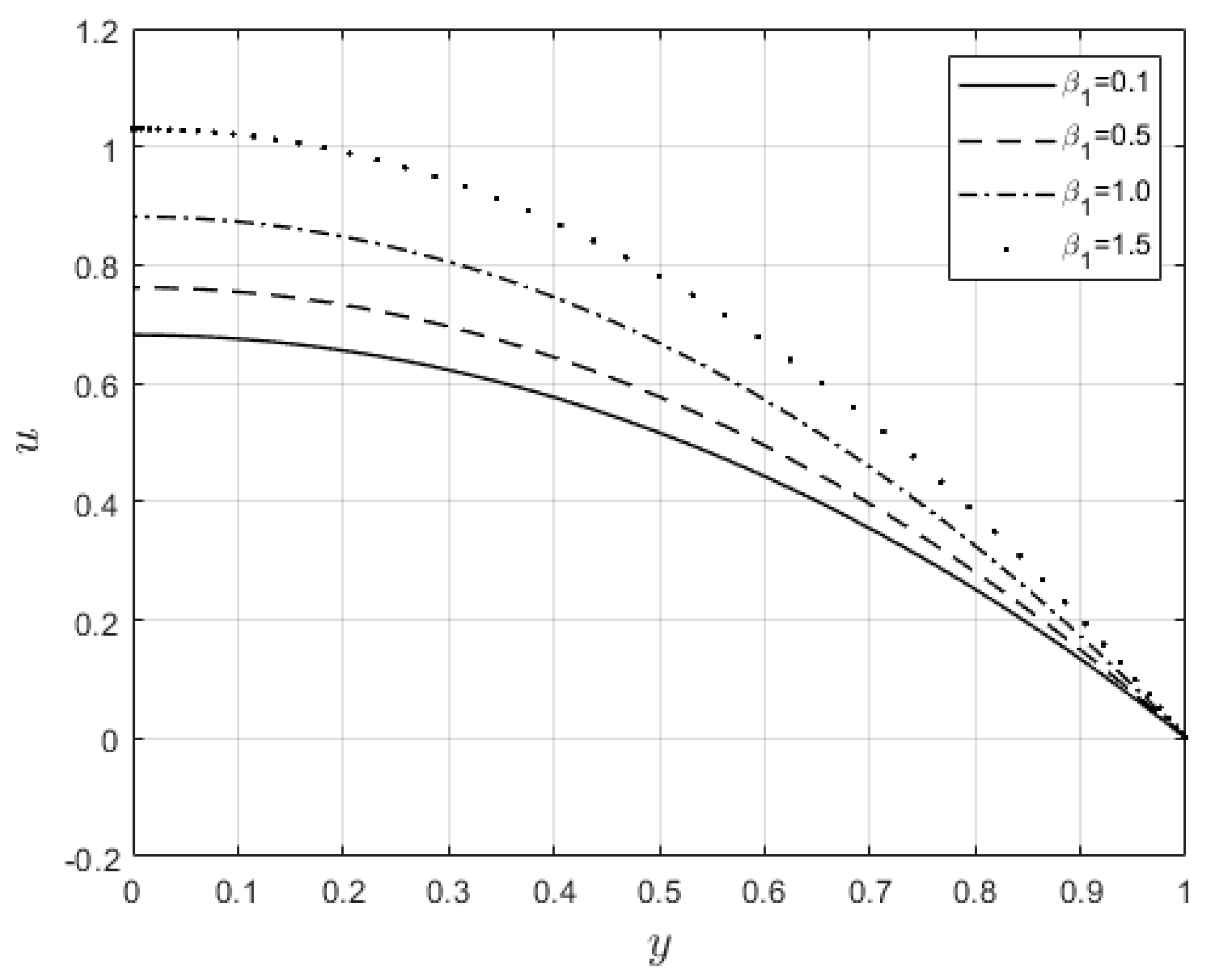
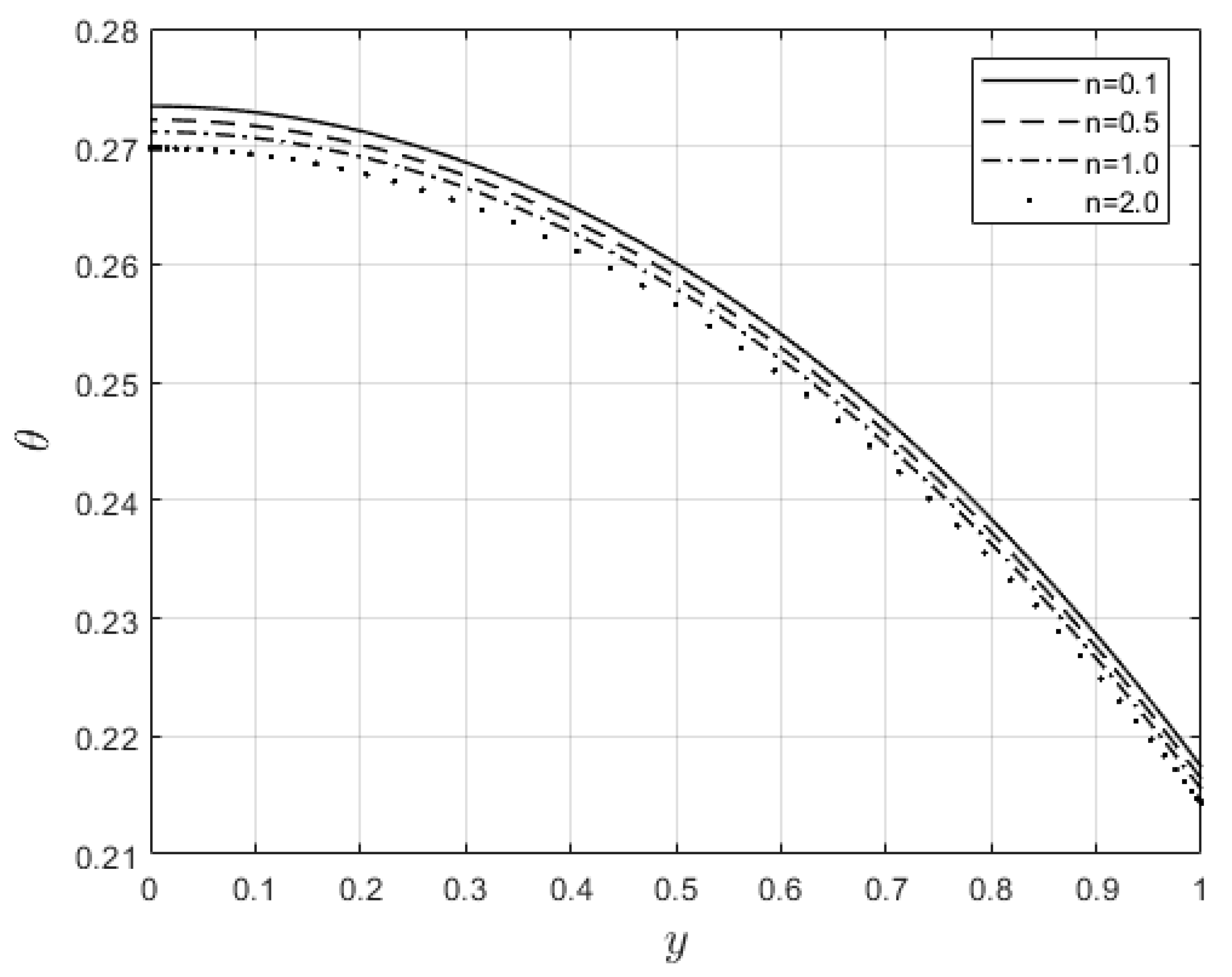
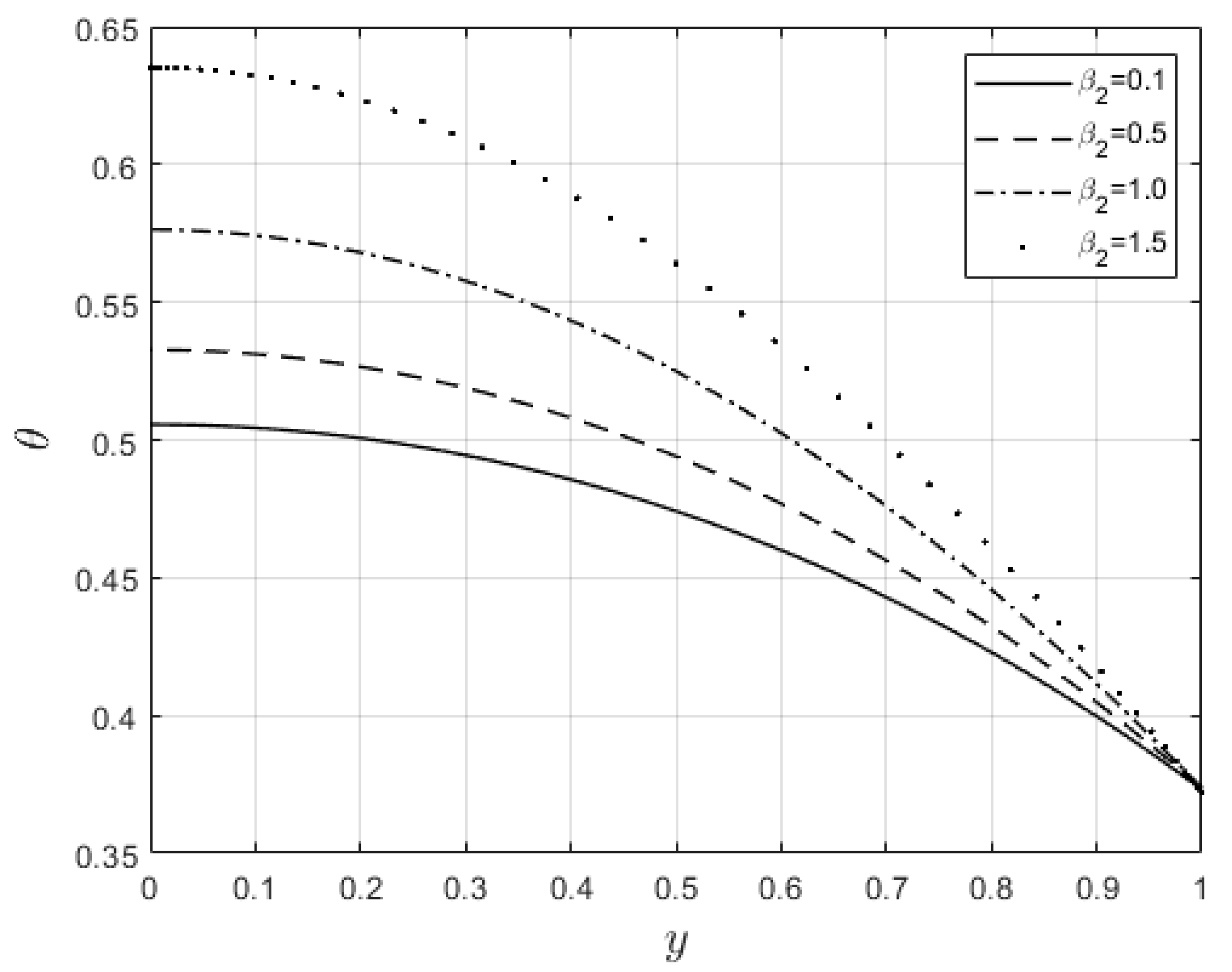
4.3. Dependence of Velocity and Temperature Profiles on Flow Parameters

Figure 6 and Figure 7 depict the impacts of $W_e$ on the velocity and temperature profiles, respectively. Both profiles are elevated as the $W_e$ values increase. This is ascribed to the fact that an increase in $W_e$ makes the fluid thinner, and the resistance force to the flow decreases; hence, the velocity profile increases. Furthermore, internal heat generation, as a result of the viscous term, is high when $W_e$ increases. This leads to an enhancement of the temperature profile. Figure 8 and Figure 9 present the effect of the power law index, $n$, on the velocity and temperature distributions, respectively. As such, the velocity distribution decreases with increasing $n$ values. When $n>1$, the resistance force to the flow for shear-thickening fluids becomes maximal, and the velocity profile decreases (see Figure 8). A decrease in fluid speed results in a decrease in viscous heating, and the temperature profile reduces significantly (see Figure 9).

Figure 10 and Figure 11 examine the behavior of velocity and temperature distributions subjected to a variable viscosity parameter, ${\beta }_1$. The velocity profile is elevated with increasing values of ${\beta }_1$, as observed in Figure 10. The reason for this is that fluid viscosity reduces as ${\beta }_1$ increases, and the kinetic energy of the fluid molecules increases, leading to velocity distribution enhancement. An increase in the velocity profile naturally enhances the heat source term in the energy equation, resulting in an elevation in the temperature field (see Figure 11). The impact of variable thermal conductivity, ${\beta }_2$, on the velocity and temperature distributions is provided in Figure 12 and Figure 13, respectively. An increase in the values of ${\beta }_2$ increases the temperature profile (see Figure 13). This is attributed to the fact that a rise in ${\beta }_2$ leads to a reduction in the thermal conductivity term, $e^{-{\beta }_2\theta }$. This leads to the slow, random movement of fluid molecules and thus facilitates heat transfer through the fluid, which consequently enhances the temperature profile. A significant rise in temperature as ${\beta }_2$ increases results in a reduction in the fluid viscosity and thus enhances the flow speed (see Figure 12). Figure 14 depicts the impact of the radiation parameter, $Ra$, on the fluid temperature. It can be observed that the temperature profile reduces as the $Ra$ values rise. This indicates that more heat exits the stockpile through radiation and, thus, reduces the fluid temperature profile. The same scenario is seen in Figure 15 as the temperature profile reduces with an increasing Biot number, $Bi$, because more heat escapes the stockpile through the walls. Enhancement in the temperature profile is observed in Figure 16 as the two-step parameter, $\omega$, values increase. This is due to extra heating created by higher values of $\omega$. Figure 17 and Figure 18 illustrate the variation in the Nusselt number, Nu (heat transfer rate at the wall) for different combinations of thermophysical parameters. Nu increases with higher values of the Frank–Kamenetskii parameter, $\lambda$, and the two-step reaction parameter, $\omega$, and decreases with higher values of the radiation parameter, $Ra$, and the Biot number, $Bi$. These results agree with the work in [32].

5. Concluding Remarks

This article considered the combustion of polymer material in a rectangular stockpile. The rheology of the polymer was assumed to follow a Carreau fluid constitutive relation. The spectral local linearization method was implemented to provide a numerical solution to the problem. The impacts of various thermokinetics factors on the flow and thermal behaviors were examined. From the obtained results, it was found that some parameters ($W_e, {\beta }_2, and \omega$) improve the combustion process since the temperature profiles increase as the values of these parameters increase. This may speed up thermal ignition and, thus, lead to an explosion. The opposite case can be observed for an increase in the values of $n, Ra, and Bi$. This slows down the chemical reaction and, thus, minimizes the combustion process.

References

1. Xiong, Q.; Kong, S. Modelling effect of interphase transport coefficients on biomass pyrolysis in fluidized beds. Powder Technol. 2014, 262, 96–105. [Google Scholar]
2. Xiong, Q.; Kong, S.; Passalacqua, A. Development of a generalized numerical frame work for simulating biomass fast pyrolysis in fluidized-bed reactors. Chem. Eng. Sci. 2013, 99, 305–313. [Google Scholar]
3. Tan, Z.; Su, G.; Su, J. Improved lumped models for combined convective and radiative cooling of a wall. Appl. Therm. Eng. 2009, 29, 2439–2443. [Google Scholar]
4. Drysdale, D. Ignition: The initiation of flaming combustion. In An Introduction to Fire Dynamics, 3rd ed.; Wiley: Hoboken, NJ, USA, 2011; Chapter 6; pp. 225–275. [Google Scholar]
5. Shi, L.; Chew, M.Y.L. A review of fire processes modeling of combustible materials under external heat flux. Fuel 2013, 106, 30–50. [Google Scholar]
6. Sener, A.A.; Demirhan, E. The investigation of using magnesium hydroxide as a flame retardant in the cable insulation material by cross-linked polyethylene. Mater. Des. 2008, 29, 1376–1379. [Google Scholar]
7. Gong, T.; Xie, Q.; Huang, X. Fire behaviors of flame-retardant cable part decomposition, swelling and spontaneous ignition. Fire Saf. J. 2018, 95, 113–121. [Google Scholar]
8. Xie, Q.; Gong, T.; Huang, X. Fire Zone Diagram of Flame-Retardant Cables: Ignition and Upward Flame Spread. Fire Technol. 2021, 57, 2643–2659. [Google Scholar]
9. Geschwindner, C.; Goedderz, D.; Li, T.; Köser, J.; Fasel, C.; Riedel, R.; Altstädt, V.; Bethke, C.; Puchtler, F.; Breu, J.; et al. Investigation of flame retarded polypropylene by high-speed planar laser-induced fluorescence of OH radicals combined with a thermal decomposition analysis. Exp. Fluids 2020, 61, 30. [Google Scholar]
10. Lohrer, C.; Krause, U.; Steinbach, J. Self-Ignition of Combustible Bulk Materials Under Various Ambient Conditions. Process. Saf. Environ. Prot. 2000, 83, 145–150. [Google Scholar]
11. Lohrer, C.; Schmidt, M.; Krause, U. A study on the influence of liquid water and water vapor on the self-ignition of lignite coal-experiments and numerical simulations. J. Prev. Process. Ind. 2005, 18, 167–177. [Google Scholar]
12. Lebelo, R.S. Thermal stability investigation in a reactive sphere of combustible material. Adv. Math. Phys. 2016, 2016, 9384541. [Google Scholar]
13. Lebelo, R.S.; Makinde, O.D.; Chinyoka, T. Thermal decomposition analysis in a sphere of combustible materials. Adv. Mech. Eng. 2017, 9, 1–14. [Google Scholar]
14. Lebelo, R.S.; Adeosun, A.T.; Gbadeyan, J.A.; Akindeinde, S.O. On the heat transfer stability for a convective reactive material of variable thermal conductivity in a sphere. Gorteria J. 2021, 34, 62–74. [Google Scholar]
15. Lebelo, R.S.; Moloi, K.C.; Okosun, K.O.; Mukamuri, M.; Adesanya, S.O.; Muthuvalu, M.S. Two-step low-temperature oxidation for thermal stability analysis of a combustible sphere. Alex. Eng. J. 2018, 57, 2829–2835. [Google Scholar]
16. Lebelo, R.S.; Waetzel, M.; Mahlobo, R.K.; Moloi, K.C.; Adesanya, S.O. On transient heat analysis of a two-step convective reactive cylinder. J. Phys. Conf. Ser. 2021, 1730, 012141. [Google Scholar]
17. Khan, M.; Hashim. Boundary layer flow and heat transfer to Carreau fluid over a nonlinear stretching sheet. AIP Adv. 2015, 5, 107203. [Google Scholar]
18. Siska, B.; Bendova, H.; MacHak, I. Terminal velocity of non-spherical particles falling through a Carreau model fluid. Chem. Eng. Process 2005, 44, 1312–1319. [Google Scholar]
19. Reedy, S.; Srihari, P.; Ali, F.; Naikoti, K. Numerical analysis of Carreau fluid flow over a vertical porous microchannel with entropy generation. Partial. Differ. Equ. Appl. Math. 2022, 5, 100304. [Google Scholar]
20. Abbas, T.; Rehman, S.; Shah, R.A.; Idrees, M.; Qayyum, M. Analysis of MHD Carreau fluid flow over a stretching permeable sheet with variable viscosity and thermal conductivity. Physical A 2020, 551, 124225. [Google Scholar]
21. Megahed, M. Carreau fluid flow due to nonlinearly stretching sheet with thermal radiation, heat flux, and variable thermal conductivity. Appl. Math. Mech. 2019, 40, 1615–1624. [Google Scholar]
22. Hayat, T.; Yasmin, H.; Alsaedi, A. Peristatic motion of Carreau fluid in a channel with convective boundary conditions. Appl. Bionics Biomech. 2014, 11, 157–168. [Google Scholar]
23. Alqarni, M.M.; Riaz, A.; Firdous, M.; Lali, I.U.; El Sayed, M.; El-Din, T.; ur Rahman, S. Hall currents and EDL effects on multiphase wavy flow of Carreau fluid in a microchannel having oscillating walls: A numerical study. Front. Phys. 2022, 10, 984277. [Google Scholar] [CrossRef]
24. Noreen, S.; Kausar, T.; Tripathi, D.; Ain, Q.U.; Lu, D. Heat transfer analysis on creeping flow Carreau fluid driven by peristaltic pumping in an inclined asymmetric channel. Therm. Sci. Eng. Prog. 2020, 17, 100486. [Google Scholar] [CrossRef]
25. Asha, S.K.; Beleri, J. Peristatic flow of Carreau nanofluid in presence of joule heat effect in an inclined asymmetric channel by multi-step differential transformation method. World Sci. News Int. J. 2022, 164, 44–63. [Google Scholar]
26. Qayyum, M.; Abbas, T.; Afzal, S.; Saeed, S.T.; Akgül, A.; Inc, M.; Mahmoud, K.H.; Alsubaie, A.S. Heat transfer analysis of unsteady MHD Carreau fluid flow over a stretching/shrinking sheet. Coatings 2022, 12, 1661. [Google Scholar]
27. Shao, Y.; Wu, A.; Abbas, S.; Khan, W.; Ashraf, I. Thermal management for the shear-rate driven flow of Carreau fluid in a ciliated channel. Int. Commun. Heat Mass Transf. 2022, 139, 106473. [Google Scholar]
28. Tshehla, M.S. The flow of a Carreau fluid down an inclined with a free surface. Int. J. Phys. Sci. 2011, 6, 3896–3910. [Google Scholar]
29. Tijani, Y.O.; Oloniiju, S.D.; Kasali, K.B.; Akolade, M.T. Nonsimilar solution of a boundary layer flow of a Reiner–Philippoff fluid with nonlinear thermal convection. Heat Transf. 2022, 51, 5659–5678. [Google Scholar]
30. Agbaje, T.; Mondal, S.; Motsa, S.; Sibanda, P. A numerical study of unsteady non-Newtonian Powell-Eyring nanofluid flow over a shrinking sheet with heat generation and thermal radiation. Alex. Eng. J. 2017, 56, 81–91. [Google Scholar]
31. Magagula, V.M. On the multidomain bivariate spectral local linearization method for solving systems of nonlinear boundary layer partial differential equations. Int. J. Math. Math. Sci. 2019, 2019, 6423294. [Google Scholar]
32. Tairu, S.; Makinde, O.D. Analysis of nonlinear heat transfer in a cylindrical solid with two-step exothermic kinetic and radiative heat loss. Defect Diffus. Forum 2017, 377, 17–28. [Google Scholar]
Figure 1. Problem physical geometry.
Mathematics 11 03510 g001
Figure 2. (a) Solution convergence against the number of iterations. (b) Residual errors against the number of iterations.
Mathematics 11 03510 g002
Figure 3. (a): Velocity steady state condition. (b): Temperature steady state condition.
Mathematics 11 03510 g003
Figure 4. (a) Three-dimensional velocity profile. (b) Three-dimensional temperature profile.
Mathematics 11 03510 g004
Figure 5. Bifurcation curve.
Mathematics 11 03510 g005
Figure 6. Velocity distributions for W e .
Mathematics 11 03510 g006
Figure 7. Temperature distribution for W e .
Mathematics 11 03510 g007
Figure 8. Velocity profiles for n .
Mathematics 11 03510 g008
Figure 9. Temperature profiles for n .
Mathematics 11 03510 g009
Figure 10. Velocity graph for variation in β 1 .
Mathematics 11 03510 g010
Figure 11. Temperature graph for variation in β 1 .
Mathematics 11 03510 g011
Figure 12. β 2 effect on velocity profiles.
Mathematics 11 03510 g012
Figure 13. β 2 effect on temperature profiles.
Mathematics 11 03510 g013
Figure 14. Impact of R a on temperature distribution.
Mathematics 11 03510 g014
Figure 15. Influence of B i on temperature profiles.
Mathematics 11 03510 g015
Figure 16. Temperature profiles with change in ω .
Mathematics 11 03510 g016
Figure 17. Influence of R a and λ on the Nusselt number.
Mathematics 11 03510 g017
Figure 18. Influence of B i and ω on the Nusselt number.
Mathematics 11 03510 g018