Mathematical Model of the Flow in a Nanofiber/Microfiber Mixed Aerosol Filter

Abstract

A new mathematical model of an aerosol fibrous filter, composed of a variety of nano- and microfibers, is developed. The combination of nano- and microfibers in a mixed-type filter provides a higher overall quality factor compared with filters with monodisperse fibers. In this paper, we propose a mathematical model of the flow of an incompressible fluid in a porous region consisting of a set of cylinders of various diameters in the range of nano- and micrometers to describe a mixed-type aerosol filter. The flow domain is a rectangular periodic cell with one microfiber and many nanofibers. The motion of the carrier medium is described by the boundary value problem in Stokes flow approximation with the no-slip boundary condition for microfibers and the slip condition for nanofibers. The boundary element method taking into account the slip and non-slip conditions is developed. The calculated velocity field, streamlines, vorticity distribution, and drag of separate fibers and the entire periodic cell are presented. Numerical results for the drag force of the porous medium of a mixed-type filter for the various ratios of mass proportion of nano- and microfibers, porosity, and filtration velocity are presented. The obtained results are compared with the analytical formulas based on the approximate theory of filtration of bimodal filters and with known experimental data. It is shown that with an increase in the mass fraction of nanofibers, the total drag force of the cell increases, while the relative contribution of nanofibers to the total drag force tends toward the value that is less than unity. An approximate analytical formula for the drag coefficient of a mixed aerosol filter is derived. The developed flow model and analytical formulas allow for estimating the aerodynamic drag of a mixed filter composed by nano- and microfibers.

1. Introduction

Filters that consist of many randomly arranged cylindrical fibers, where suspended particles are trapped as a result of diffusion deposition or inertial impaction, are widely used to clean the air from aerosol pollution. A theoretical description of the main mechanisms of capture of suspended particles in aerosol filters is given in works [1,2,3,4,5,6,7].

The calculation of the performances of filters is based on the mathematical modeling of the flow of aerosol through the porous structure of the filter. In the dependence on the size range of aerosol particles, their motion is described by the Euler or Lagrangian transport equations in a known velocity field of the carrier medium. One of the widely used flow models in aerosol filters is the so-called Kuwabara cell analytical model [8] that is the Stokes flow of an incompressible liquid in a periodic cell of cylindrical fibers. The circular cell approximation model was used in [9,10,11]. Along with the Kuwabara model, various numerical models of flows in fibrous filters are developed in [12,13,14,15,16,17,18,19,20,21,22,23,24,25,26,27,28,29,30]. Flows for regular and irregular configurations of porous structures and various Reynolds numbers were studied, including CFD codes.

Most of the previous studies relate to aerosol fibrous filters of a monodisperse composition with micro- or nanofibers. Aerosol nanofiber filters have a significant advantage over microfiber filters due to their lower aerodynamic drag, with an efficient capture of particles as a result of the diffusion deposition mechanism. Various production methods, such as melt-blown, electrospinning, and stretching of polymer films, have been developed to obtain nanofibers for aerosol filter medium [31,32,33]. The basic principles of air filtration using the complex-structured nanofibers are discussed in the review of [34]. The results of experimental measurements of the collection efficiency of nanofiber filters were presented in [35]. The pressure drop in nanofiber filters was studied in [36,37,38,39]. Theoretical studies’ results for nanofiber filters were given in [28,36,40,41,42,43,44]. It was mentioned also in [45] that the particle capture efficiency of nanofiber filters is not as high as expected by the filtration theory because of the nonuniform packing of fibers. In [45], the collection performance of nanofiber/microfiber composite filters was experimentally studied, in which nanofibers are well dispersed among micrometer fibers. It has been shown that the combination of the advantages of high efficiency of capture of aerosol particles and low aerodynamic drag of nanofibers and controlled homogeneity of microfibers allows mixed filters to provide a higher overall filter quality factor as compared with filters with monodisperse fibers. In [45], the analytical formulas from the theory of filtration for a bimodal aerosol filter [46] are used for the calculation of the drag and particle capture efficiency. Strictly speaking, the mentioned formulas are not applicable in the case of a mixed-type filter. Presently, the question of a rigorous theoretical description of hydrodynamic processes in a mixed-type filter remains open.

To close the mentioned gap in the theoretical study of mixed filters, a mathematical model of flow in a porous medium composed of nano- and microfibers is developed. The paper includes chapters with a mathematical formulation of the problem and obtained numerical results. The proposed mathematical model of the flow of an incompressible viscous fluid in a porous region describes a fluid flow in a rectangular periodic cell with one microfiber and many nanofibers. The approximation of the Stokes flow with the no-slip boundary condition for microfibers and the slip condition for nanofibers is applied. The boundary element method is developed to find the velocity field, streamlines, and vorticity distribution. Numerical parametrical studies of aerodynamic drag and a comparison with experimental data are presented. The approximate analytical formula for the drag of a mixed filter is derived.

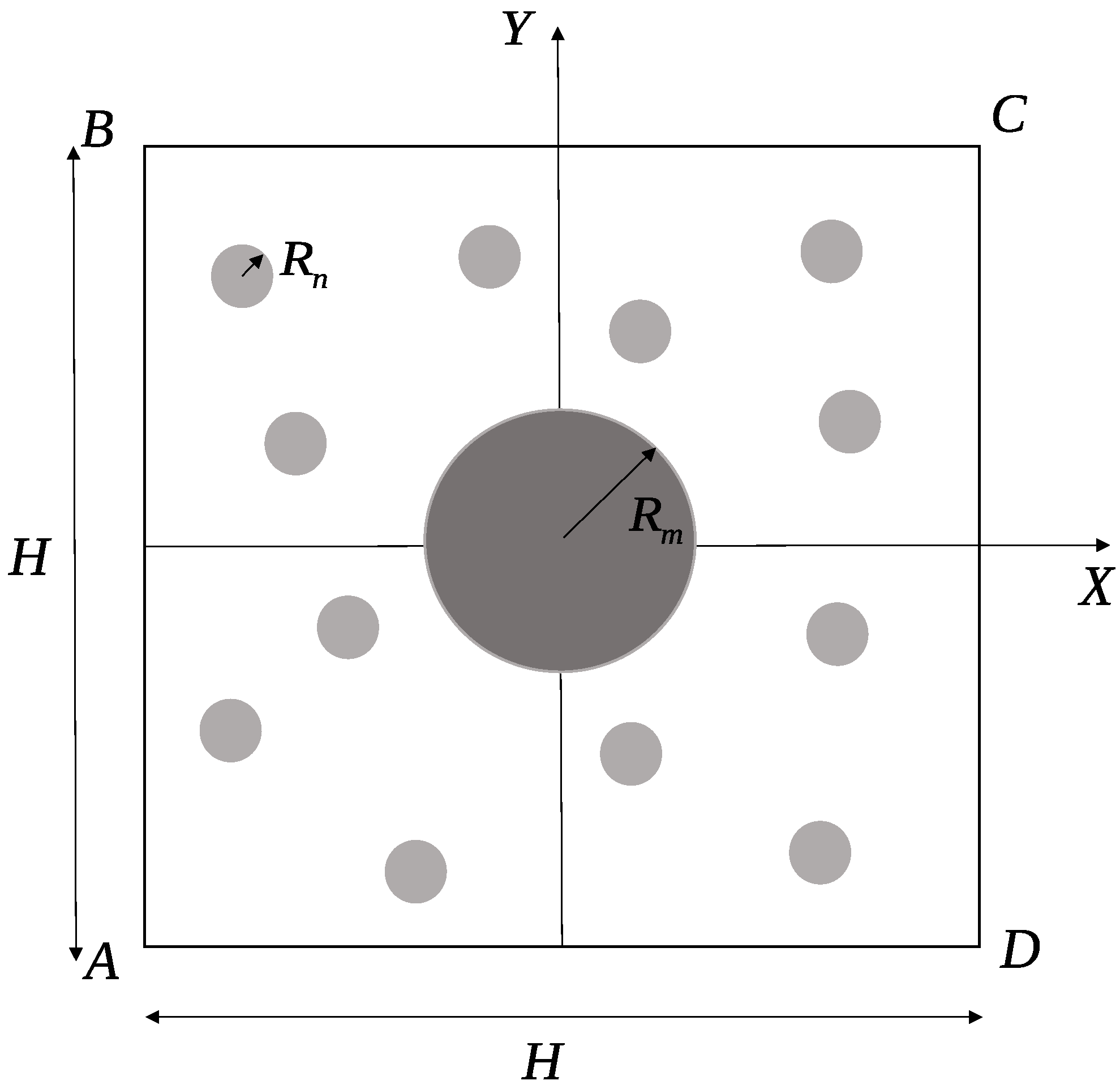
2. Formulation of the Problem

To simulate the flow of a viscous fluid in a mixed filter consisting of parallel solid inclusions of a cylindrical shape, let us select a square periodic cell with a side H (Figure 1). In the center of the cell, a microfiber of a radius $R_m$ is located. The rest of the cell volume is occupied by N nanofibers, each of a radius $R_n$, which are located randomly. A common fiber packing density $\alpha$ is defined as the ratio of the volume $V_f$ of all fibers to the cell volume V [7]:

$$\alpha =\frac{V_f}{V}.$$

(1)

For a 2d fluid flow problem, taking into account that the element size is equal to unity in the direction perpendicular to the plane, we can rewrite the last relation in the form

$$\alpha =\frac{\pi R_m^2+N\pi R_n^2}{H^2}=\frac{\pi R_m^2}{H^2}\frac{N+k^2}{k^2},$$

(2)

where $k=R_m/R_n$ is the ratio of the microfiber to the nanofiber radii. The mass fraction $\gamma$ of nanofibers is the ratio of the mass $M_n$ of nanofibers to the total mass of fibers:

$$\gamma =\frac{M_n}{M_n+M_m},$$

where $M_m$ is the microfiber mass. Assuming the same density of nano- and microfibers, we write the value of $\gamma$ in the form

$$\gamma =\frac{N\pi R_n^2}{N\pi R_n^2+\pi R_m^2}=\frac{N}{N+k^2}.$$

(3)

For the known $R_m$, k, and $\alpha$ from the relations (1) and (3), we obtain the expressions for the height H of the periodic cell and the number N of nanofibers:

$$H=\sqrt{\frac{\pi }{\alpha (1-\gamma )}}{R}_m,$$

(4)

$$N=\frac{\gamma k^2}{1-\gamma }.$$

(5)

Figure 1. Square periodic cell of mixed filter.

Choosing the cell size H and the average flow velocity $U_0=Q/H$ (Q is the gas flow rate through the cell) and the fluid viscosity $\mu$ as the characteristic dimensional quantities, the problem of a slow flow of a viscous fluid in a considered periodic cell in the Stokes approximation [47] is formulated in the dimensionless form. Further, all dimensionless quantities will be written by small letters. The flow equations are written as

$$-\overrightarrow{\nabla }p+\Delta \overrightarrow{u}=0,$$

(6)

$$\mathrm{div}\overrightarrow{u}=0,$$

where $\overrightarrow{u}=(u_x,u_y)$ is the velocity vector, and p is the pressure. We introduce the flow stream function $\psi (x,y)$ and vorticity $\omega$ by the relations

$$u_x=\frac{\partial \psi }{\partial y},u_y=-\frac{\partial \psi }{\partial x},$$

(7)

$$\omega =\frac{\partial u_y}{\partial x}-\frac{\partial u_x}{\partial y}.$$

The components $u_x$, $u_y$ of the flow velocity vector can be expressed through the vorticity $\omega$ as

$$\Delta u_x=-\frac{\partial \omega }{\partial y},\Delta u_y=\frac{\partial \omega }{\partial x}.$$

(8)

Equation (6) can be rewritten as

$$\left\{\begin{array}{c}{\displaystyle \frac{\partial p}{\partial x}=-\frac{\partial \omega }{\partial y},}\hfill \\ {\displaystyle \frac{\partial p}{\partial y}=\frac{\partial \omega }{\partial x}.}\hfill \end{array}\right.$$

(9)

Differentiating the first Equation (9) with respect to y and the second with respect to x, and subtracting one from the other, we write

$$\Delta \omega =0.$$

(10)

From (7) and (8), it follows that

$$\omega =-\Delta \psi .$$

(11)

Taking this into account (11), we obtain that the stream function satisfies the biharmonic equation

$${\Delta }^2\psi =0.$$

Let us formulate the boundary conditions for the system of Equations (10) and (11). On the sides $AB$ and $CD$ of a periodic cell, we set the conditions of periodicity:

$$\frac{\partial \psi }{\partial n}=0,\frac{\partial \omega }{\partial n}=0,$$

(12)

where n is the direction of the outer normal to the boundary of the flow region. On the sides $BC$ and $AD$, we accept the symmetry conditions

$$\psi =\pm \frac{1}{2},\omega =0.$$

(13)

On the microfiber surface, the no-slip condition is taken:

$$u_n=0,u_{\tau }=0,$$

(14)

where $u_n$, $u_{\tau }$ are the normal and tangential velocity components.

The air flow regime around the nanofibers is determined by the Knudsen number:

$$\mathrm{Kn}=\frac{L_0}{R_n},$$

(15)

where $L_0$ is the mean free path of molecules. For nanofibers in the case of small Knudsen numbers, the $\mathrm{Kn}<0.25$ [48] calculation of the flow of a viscous fluid around fibers can be made within the framework of continuum mechanics with a slip condition on the fiber surface. The widely used slip condition for the flow problem around nanospheres was proposed in [49,50]. The tangential slip velocity $u_{\tau }$ is assumed to be proportional to the shear stress ${\tau }_t$ on the body surface:

$$u_{\tau }=\lambda r_n{\tau }_t,$$

(16)

where $\lambda =f\left(\mathrm{Kn}\right)$ is the slip coefficient determined by the interaction of the gas with the surface, $r_n=R_n/H$. The condition (16) has been accepted in most previous studies. The slip coefficient $\lambda$ is usually assumed to be proportional to the Knudsen number:

$$\lambda =\xi \mathrm{Kn},$$

where the coefficient $\xi$ is close to unity. Further, following [51], let us take $\xi =1.147$. In [52], a modified slip condition is proposed. The tangential velocity is assumed to be proportional to the vorticity value and nanofiber radius:

$$u_{\tau }=\lambda r_n\omega .$$

(17)

In [52], it was shown that the condition (17) provides a better agreement with experiments. The slip condition (17) and impermeability condition,

$$u_n=0,$$

(18)

are taken on the surface of each nanofiber. The boundary value problem (10)–(14), (17) and (18) is solved numerically using the boundary element method. A description of the applied method is given in [53,54]. The method is realized in Fortran. The average time of computations for one variant is 5 min on our PC (CPU AMD Ryzen 9 5950X 16x3.4GHz, RAM 64 Gb).

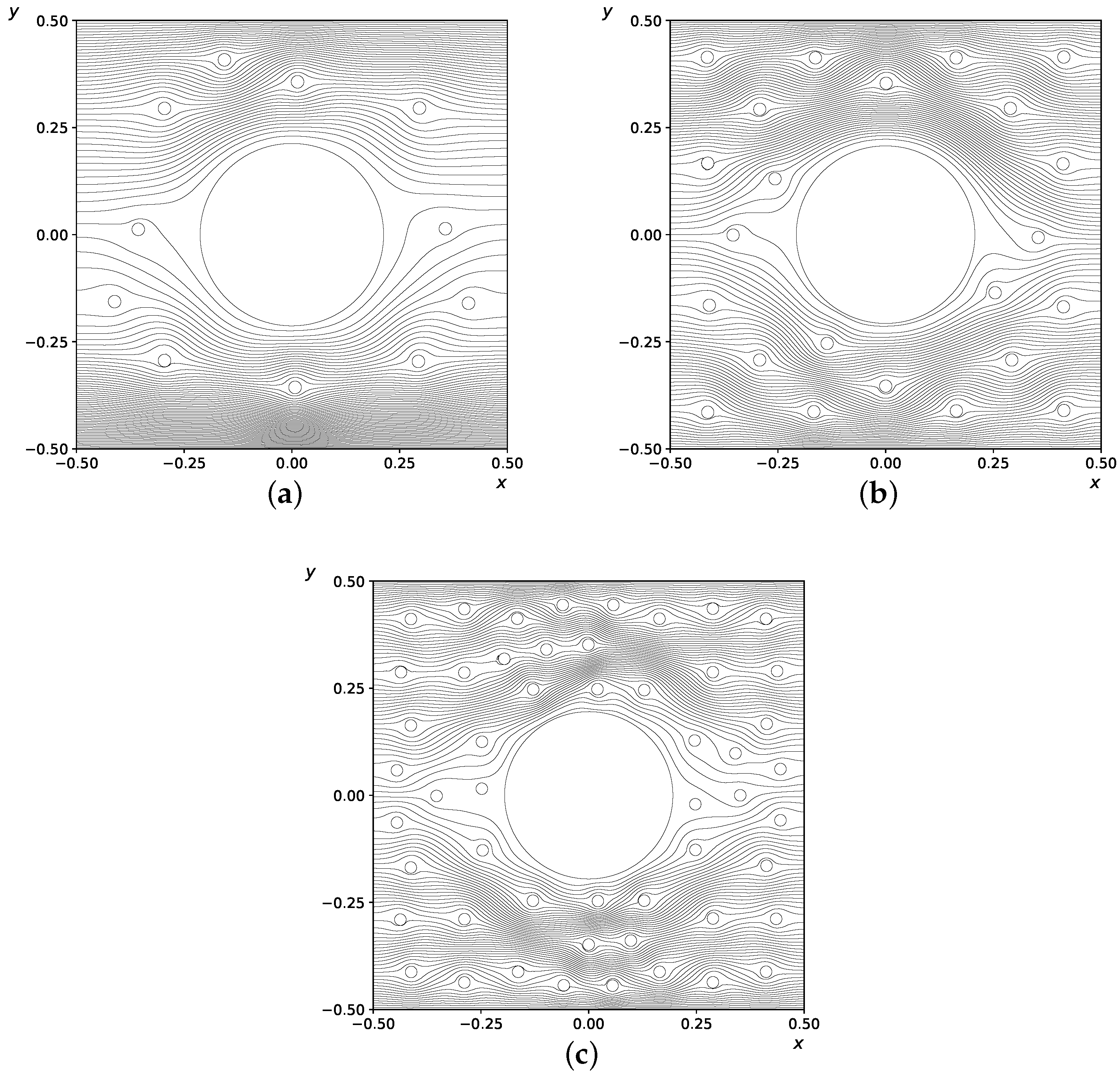
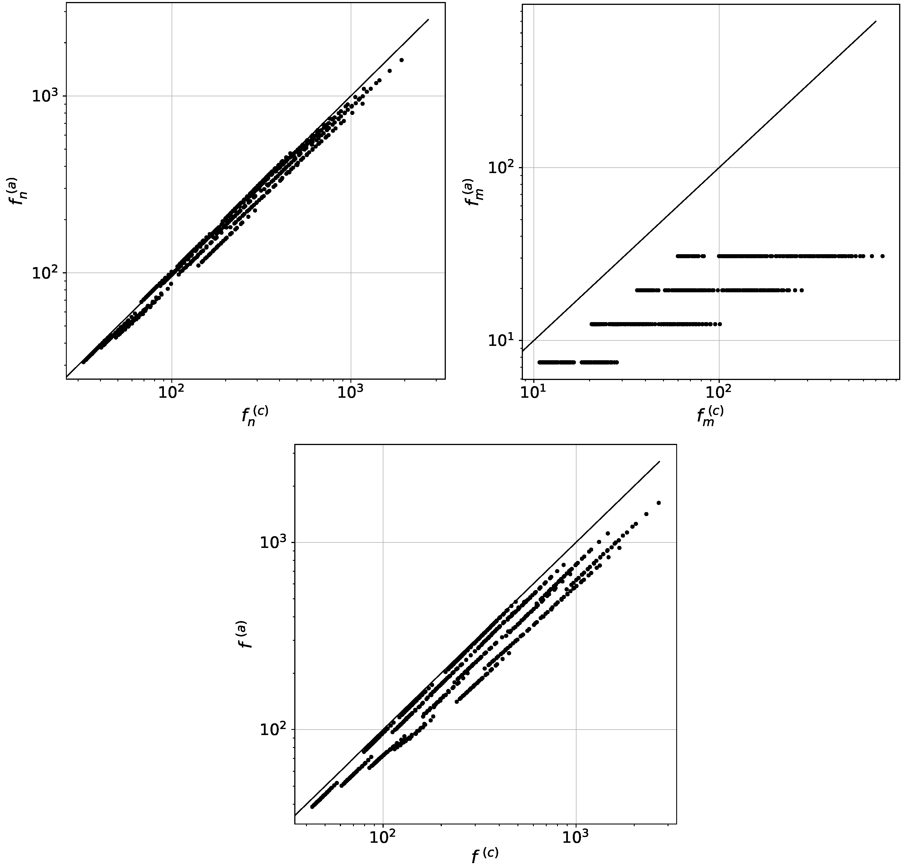
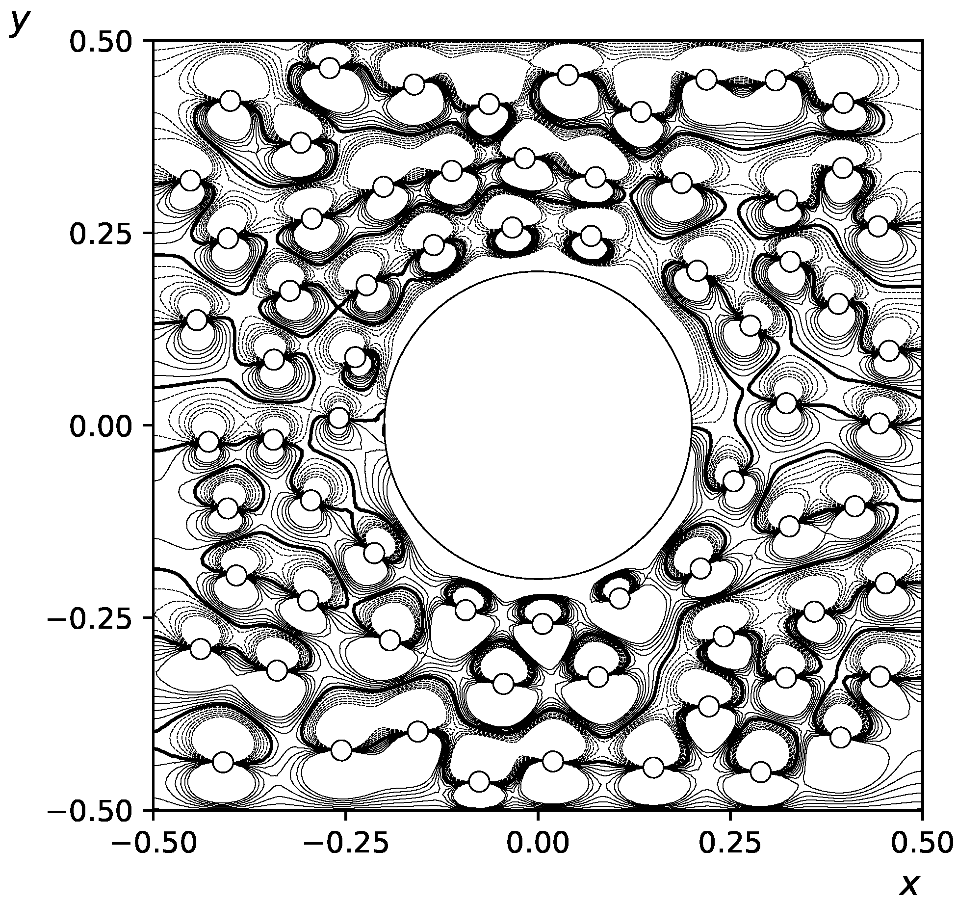
3. Numerical Results

To calculate the aerodynamic drag of the considered periodic element with a microfiber and many nanofibers, using the obtained numerical solution of the Stokes problem, two approaches were used. The first approach is based on the integration of shear stresses over the surface of each fiber. To calculate the drag force $f_i$ acting on an arbitrary circular fiber, we introduce a local polar coordinate system $(r,\theta )$ with the center that is located in the center of the fiber. The angle $\theta$ will be counted from the horizontal axis counterclockwise. Then the drag force $f_i$ of the i-th fiber of a radius $r_i$ is written as

$$f_i=\underset{{\mathrm{\Gamma }}_i}{\int }({\tau }_{rr}cos\theta -{\tau }_{r\theta }sin\theta )dg=\underset{0}{\overset{2\pi }{\int }}({\tau }_{rr}cos\theta -{\tau }_{r\theta }sin\theta )r_{i}d\theta ,$$

(19)

where g is the arc length of the nanofiber ${\mathrm{\Gamma }}_i$. The components ${\tau }_{rr},{\tau }_{r\theta }$ of the stress tensor in the polar coordinates have the form

$${\tau }_{rr}=-p+2\frac{\partial u_r}{\partial r},$$

$${\tau }_{r\theta }=\frac{1}{r}\frac{\partial u_r}{\partial \theta }+\frac{\partial u_{\theta }}{\partial r}-\frac{u_{\theta }}{r}.$$

To determine the pressure, we write the projection of (6) onto a tangential direction:

$$\frac{1}{r}\frac{\partial p}{\partial \theta }=\Delta u_{\theta }-\frac{u_{\theta }}{r^2}+\frac{2}{r^2}\frac{\partial u_r}{\partial \theta }$$

and integrate it for $r=r_i$. We find the drag of nanofibers by the formula

$$f_n=\sum _{i=1}^N{f}_i.$$

(20)

Then the total drag force of the entire periodic element will be written as

$$f=f_m+f_n.$$

(21)

In the framework of the second approach, we write for the periodic element:

$$f=\Delta ps=\Delta p,$$

where $\Delta p=p_{AB}-p_{CD}$ is the pressure difference between the side faces of the cell, and s is a dimensionless area of the side face of the cell, which in the two-dimensional case is equal to the height of the periodic cell $h=1$. To calculate the pressure drop from the first Equation (9), we write the formula

$$\Delta p=-\underset{l}{\int }\frac{\partial p}{\partial x}dx=\underset{l}{\int }\frac{\partial \omega }{\partial y}dx,$$

where the integration is carried out along the curve l, the ends of which have the coordinates $\left(-1/2,y_0\right)$ and $\left(1/2,y_1\right)$, $\left(-1/2⩽y_0,y_1⩽1/2\right)$, and the curve itself does not cross the boundaries of any solid inclusion.

The first approach allows us to calculate the contribution of each fiber separately to the total drag force, while the second approach evaluates the total drag force only. Two described approaches are used to check the accuracy of the numerical solution.

In mixed filters, both microfibers and nanofibers are located randomly in a general packing. To form a random distribution of nanofibers around a microfiber in a periodic cell, the method of the best candidate Mitchell [55] was used. In Figure 2, the streamlines of flow in a periodic element for the values of the parameters $\lambda =0.1$, $\alpha =0.15$, $k=14.36$ and various mass fractions $\gamma =0.05$ (a), $0.1$ (b), $0.2$ (c) are presented.

Figure 2. Streamlines for various mass fractions of $\gamma$ nanofibers at $\lambda =0.1$, $\alpha =0.15$, $k=14.36$: (a) $\gamma =0.05$, (b) $\gamma =0.1$, (c) $\gamma =0.2$.

In [45], the analytical formulas are proposed for calculating the drag force of the mixed filter, separately taking into account the contribution of micro- and nanofibers:

$$f_m=\frac{4\pi }{k_0\left({\alpha }_m\right)},f_n=\frac{4\pi N}{k_1\left({\alpha }_n\right)},$$

(22)

where

$$k_0\left(\alpha \right)=-0.5ln\alpha -0.75+\alpha -0.25{\alpha }^2,$$

$$k_1\left(\alpha \right)=k_0\left(\alpha \right)+{(1-\alpha )}^2\lambda$$

is the so-called Kuwabara hydrodynamic factor $k_0$ and $k_1$ without and with taking into account the slip on the surface of micro- and nanofibers, respectively. For the determination of the packing densities ${\alpha }_m$ and ${\alpha }_n$ of micro- and nanofibers in [45], it was assumed that they are proportional to the mass fractions:

$${\alpha }_m=\alpha (1-\gamma ),{\alpha }_n=\alpha \gamma .$$

(23)

Taking into account the expressions for the packing density and mass fraction of nanofibers (2) and (3), the expression (23) can be written as ($r_m=R_m/H$):

$${\alpha }_m=\pi r_m^2,{\alpha }_n=\frac{\pi r_m^{2}N}{k^2}.$$

A series of parametric calculations was carried out, in which the number of N nanofibers, radius $r_m$ of the microfiber, ratio of k radii, and slip coefficient $\lambda$ are varied. In Table 1, the values of the parameters used in the calculations are given.

Table 1. Parameters values in the calculations.

Parameter	Values
N	10, 20, 30, 50, 70
$r_m$	0.05, 0.1, 0.15, 0.2
k	10, 12.5, 15, 17.5, 20
$\lambda$	0, 0.1, 0.2, 0.3, 0.4, 0.5

The parameter values given in Table 1 allow for covering the range of mass fractions $\gamma$ from 0.025 to 0.41 and packing density range $\alpha$ from 0.008 to 0.21. The large Knudsen number for the range $0<\lambda ⩽0.5$ ($\lambda =\xi \mathrm{Kn}$) is slightly larger than the recommended range $0.01<\mathrm{Kn}<0.25$ for the slip flow model. In our previous paper [52], it was shown that the mathematical model with a new slip condition gives the linear dependence of the inverse drag force on the Knudsen number that was observed in experiments in [36,38]. In the mentioned experiments, the linear dependence on the Knudsen number was observed in a wider range (up to $\mathrm{Kn}=20$) than is recommended for the slip flow model. It means that we can use the slip flow model outside the range $0.01<\mathrm{Kn}<0.25$. For each set of parameters, 100 calculations were carried out with different random distributions of nanofibers over the area of a periodic cell. In each calculation, the total drag force f and the forces $f_m$ and $f_n$ of micro- and nanofibers were found according to Formulas (19)–(21). Then the calculated forces were averaged by the arithmetic mean formula in order to eliminate the influence of the random distribution of nanofibers.

Figure 3 shows cross-plots of a comparison of the drag forces $f^{\left(c\right)}$, $f_n^{\left(c\right)}$, and $f_m^{\left(c\right)}$ found from the numerical model with the values $f^{\left(a\right)}$, $f_n^{\left(a\right)}$, and $f_m^{\left(a\right)}$ determined from the analytical Formulas (22) and (23). Here and below, the superscripts “$\left(c\right)$” and “$\left(a\right)$” mean the value of the parameter found from the numeric model and analytical formulas. Dots in Figure 3 show the values averaged over 100 calculations of forces for a certain set of parameter values from Table 1. The number of points that correspond to the number of used parameters is six hundred. The diagonal line corresponds to the locus of points for which the values of the forces determined during the calculations coincide with the values of the forces, found by analytical formulas. It can be seen from the graphs that both the total drag forces and drag forces of the microfiber, found by the analytic Formulas (22) and (23), significantly differ from their values obtained by the numerical model.

Figure 3. Cross-plots of the drag forces $f_n^{\left(c\right)}$, $f_m^{\left(c\right)}$, and $f^{\left(c\right)}$ from the numerical model and $f_n^{\left(a\right)}$, $f_m^{\left(a\right)}$, and $f^{\left(a\right)}$ from the analytical Formulas (22) and (23). Dots show the values averaged over 100 calculations of forces for a certain set of parameter values from Table 1. The solid line corresponds to the locus of points for which the values of the forces from the numerical model coincide with the values of the analytically found forces.

The values of relative errors are determined by the formulas

$$\epsilon =\frac{f^{\left(a\right)}-f^{\left(c\right)}}{f^{\left(c\right)}}·100\%,{\epsilon }_n=\frac{f_n^{\left(a\right)}-f_n^{\left(c\right)}}{f_n^{\left(c\right)}}·100\%,{\epsilon }_m=\frac{f_m^{\left(a\right)}-f_m^{\left(c\right)}}{f_m^{\left(c\right)}}·100\%.$$

Table 2 shows the average and maximum values of modules of relative errors $\epsilon$, ${\epsilon }_n$, ${\epsilon }_m$ found for all parametric calculations. It can be seen that the Formulas (22) and (23) give $\epsilon$ greater than 20% and ${\epsilon }_m$ is almost 70%, which indicates insufficient accuracy of the model (22) and (23).

Table 2. Relative errors $\epsilon$, ${\epsilon }_n$, ${\epsilon }_m$, %.

	$\mathbf{\left|}\mathit{\epsilon }\mathbf{\right|}$	$\mathbf{|}{\mathit{\epsilon }}_{\mathit{n}}\mathbf{|}$	$\mathbf{|}{\mathit{\epsilon }}_{\mathit{m}}\mathbf{|}$
Average (22) and (23)	20.8	6.4	68.5
Maximum (22) and (23)	44.3	22.8	96
Average (24)–(27)	3.6	2.3	8.9
Maximum (24)–(27)	11.9	8	22.7

Insufficient accuracy of the analytical model (22) and (23) is connected with the unjustified determination of the quantities ${\alpha }_m$ and ${\alpha }_n$ by Formula (23) and the assumption that the velocity $u_m$ of the free stream for the microfiber and the average local free flow velocity $u_n$ for nanofibers is equal to unity, i.e., the values $u_m$ and $u_n$ coincide with the average flow velocity in the entire periodic cell.

For a more rigorous definition of ${\alpha }_m$ and ${\alpha }_n$, we consider Figure 4 that shows the isolines of the vorticity $\omega$ calculated by the numerical model in the periodic cell of the mixed filter for $N=80$, $k=15$, $r_m=0.2$, $\lambda =0.1$. The thick lines show isolines of zero vorticity $\omega =0$. On thin lines, the vorticity value is from one to five percent of the maximum and minimum values of vorticity in the local flow domain. The increments for plotting these isolines is one percent. It can be seen that each nanofiber has its own local flow area inside the line $\omega =0$, similar to the circular Kuwabara cell where the zero vorticity value at the outer boundary is accepted. Thus the calculation of the drag based on Formula (22) can be done in the assumption that a local flow is formed in the vicinity of each fiber in the area demarcated by the zero vorticity line.

Figure 4. Isolines of vorticity in the periodic cell for $N=80$, $k=15$, $r_m=0.2$, $\lambda =0.1$. The thick lines show isolines of zero vorticity $\omega =0$.

Introducing the quantities $u_m$ and $u_n$, we rewrite the Formula (22) as

$$f_m=\frac{4\pi u_m}{k_0\left({\alpha }_m\right)},f_n=\frac{4\pi N{u}_n}{k_1\left({\alpha }_n\right)}.$$

(24)

The values ${\alpha }_m$ and ${\alpha }_n$ for micro- and nanofibers will be determined using the microfiber cell area $s_m$ and average nanofiber cells areas $s_n$ according to the formulas

$${\alpha }_m=\frac{\pi r_m^2}{s_m},{\alpha }_n=\frac{\pi r_n^2}{s_n}.$$

Assuming that the area $s_m$ of a microfiber cell differs slightly from the microfiber cross-sectional area (Figure 4), we find the remaining area, occupied by the cells of nanofibers. For this purpose, we use the formula $N{s}_n=1-\pi r_m^2$. Thus, the quantity ${\alpha }_n$ can be expressed as

$${\alpha }_n=\frac{\pi r_n^{2}N}{1-\pi r_m^2}.$$

(25)

The average velocity $u_n$ of the oncoming flow in the periodic cell for nanofibers is defined as the average flow velocity outside the microfiber

$$u_n=\frac{1}{1-\pi r_m^2}.$$

(26)

The velocity $u_m$ and packing density ${\alpha }_m$, which influence the microfiber drag force $f_m$, have a complex dependence on the parameters N, $r_m$, k and $\lambda$. However, from results of numerical calculations, it was noticed that there is a close to linear dependence between the quantities $r_m\sqrt{f_n}$ and $\sqrt{f_m}$ (Figure 5).

Figure 5. Calculated values of $\sqrt{f_m}$ and $r_m\sqrt{f_n}$ (points) and linear regression (27) (line).

Based on the approximation of numerical data, the relation is obtained

$$f_m={\left(2.416+2.927r_m\sqrt{f_n}\right)}^2.$$

(27)

For parameter values from Table 1 the comparison of drag forces $f^{\left(c\right)}$, $f_n^{\left(c\right)}$, $f_m^{\left(c\right)}$ from our numerical model with values $f^{\left(a\right)}$, $f_n^{\left(a\right)}$, $f_m^{\left(a\right)}$, defined by analytic Formulas (24)–(27), is given in Figure 6. It is seen that, in contrast to Figure 3, calculations based on the numerical model and the updated analytical model give a better agreement. For individual values of the parameters, the quantity $\epsilon$, ${\epsilon }_n$, ${\epsilon }_m$ can reach 20–25%, but in average, they do not exceed $10\%$ for the estimated contributions to the drag of micro- and nanofibers and do not exceed $8\%$ for total drag (Table 2). Thus, we can conclude that the proposed analytical model can be used for approximate calculation of the drag forces of the mixed filter.

Figure 6. Cross plots of drag forces $f_n^{\left(c\right)}$, $f_m^{\left(c\right)}$, $f^{\left(c\right)}$ from the numerical model and $f_n^{\left(a\right)}$, $f_m^{\left(a\right)}$, $f^{\left(a\right)}$ from analytical Formulas (24)–(27). Dots show the values averaged over 100 calculations of forces for a certain set of parameter values from Table 1. The solid line corresponds to the locus of points for which the values of the forces from the numerical model coincide with the values of the analytically found forces.

The relative contributions of ${\varphi }_m$ and ${\varphi }_n$ of micro- and nanofibers, respectively, into the total drag force can be defined as

$${\varphi }_m=\frac{f_m}{f},{\varphi }_n=\frac{f_n}{f}.$$

(28)

Figure 7 shows the dependencies of ${\varphi }_m$ values (thick lines and square symbols) and ${\varphi }_n$ (thin lines and diamond symbols) on the mass fractions of nanofibers for $k=14.36$, $r_m=0.215$, and $\lambda =0.2$. The solid lines match the numerical model. The dashed lines correspond to the new analytical model (24)–(27) and the marks to the analytical models (22) and (23). It can be seen that with the growth of the mass fraction of nanofibers, the relative contribution ${\varphi }_n$ of nanofibers monotonically increases, while the relative contribution ${\varphi }_m$ of the microfiber monotonically decreases. Note that as $\gamma$ increases, all dependencies approach the horizontal asymptotes ${\varphi }_m={\varphi }_m^{*}$ and ${\varphi }_n={\varphi }_n^{*}$. Substituting the expression for the drag force of microfibers (27) into (28) and tending the drag force of nanofibers to infinity in the limit, we determine

$${\varphi }_m^{*}=\frac{8.6r_m^2}{1+8.6r_m^2},$$

$${\varphi }_n^{*}=\frac{1}{1+8.6r_m^2}.$$

whence for the presented example with $r_m=0.215$, the values ${\varphi }_m^{*}=0.29$ and ${\varphi }_n^{*}=0.71$ are obtained (shown in Figure 7 by dotted lines). The approximate Formulas (22) and (23) (square marks in the figure) give the limits ${\varphi }_m^{*}=0$ and ${\varphi }_n^{*}=1$. The analytical Formulas (22) and (23) do not take into account the interaction of micro- and nanofibers; therefore, they give an almost zero contribution to the microfiber drag force with a large number of nanofibers. In fact, with an increase in the number of nanofibers, the cell area for a microfiber decreases, and consequently, its drag increases. Therefore, despite the fact that the relative contribution of the microfiber drag to the total falls, this contribution will never reach zero.

Figure 7. The relative contributions of the microfiber drag ${\varphi }_m$ (thick lines and square symbols) and nanofibers ${\varphi }_n$ (thin lines and diamond symbols) to the total drag force as a function of mass fractions of nanofibers for $k=14.36$, $r_m=0.215$, and $\lambda =0.2$.

Now we compare the results derived from the proposed model with experimental data from [45], where a mixed filter with a microfiber radius $R_m=5.6$ µm and nanofiber radius $R_n=390\mathrm{nm}$ ($k=14.36$) was studied. Table 3 shows the mass fraction $\gamma$, packing density $\alpha$, and porous layer length L for four mixed filter configurations from [45]. In the experiments, the flow velocity in the filter is varied: $U_0=0.05,0.1,0.15,0.2 \mathrm{m}/\mathrm{s}$.

Table 3. Parameters for mixed filter configurations from [45].

i	$\mathit{\gamma }$	$\mathit{\alpha }$	N	$\mathit{\delta }$	L [µm]
1	0.05	0.152	11	3.2	276
2	0.1	0.172	23	2.68	237
3	0.2	0.186	52	3.27	235
4	0.3	0.195	88	1.57	239

The cell size H, calculated by Formula (4) for all four configurations, turned out to be equal to $H=26\pm 1$ µm. Then the dimensionless values of the radii of micro- and nanofibers will be $r_m=R_m/H=0.215$ and $r_n=R_n/H=0.015$, respectively. The number of N nanofibers is determined from Formula (5) for each mixed filter configuration, given in Table 3. For the mean free path of molecules in the air at normal conditions $L_0=68$ nm, the Knudsen number, calculated from Formula (15), for nanofibers is $\mathrm{Kn}=0.174$, and for microfibers, $\mathrm{Kn}=0.012$. Therefore, the slip parameter $\lambda$ in the slip boundary condition (17) for nanofibers is taken as $\lambda =0.2$. Close to zero, the value of the Knudsen number for a microfiber justifies the no-slip condition (second condition in (14)).

Taking into account that the number of periodic cells per the filter thickness L is equal to $L/H$, the dimensional value of the pressure drop across the filter is determined by the formula

$$\Delta P=\frac{f{U}_0\mu L}{H^2}.$$

The dependencies of the pressure drop $\Delta P$ calculated for L from experiments [45] on the velocity $U_0$ and on the mass fractions $\gamma$ of nanofibers are shown by solid lines in Figure 8 and Figure 9, respectively. In [45], an additional correction factor $\delta$ is also introduced to take into account the nonuniform packing of fibers in real filters:

$$\delta ={\left.\left(\frac{\Delta P^f}{\Delta P^r}\right)\right|}_{\mathrm{Kn}=0},$$

where $\Delta P^r$ is the real filter pressure drop, and $\Delta P^f$ is the pressure obtained using the fan model filter (FMF) model. The correction coefficients $\delta$ from [45] for various values of the mass fractions of the nanofibers $\gamma$ are also given in Table 3. Experimental data values from [45], multiplied by the correction factor $\delta$, are given by marks in Figure 8 and Figure 9. A qualitative agreement between the numerical and experimental data is obtained. For the mass fractions $\gamma =0.05,0.1$, a good quantitative agreement is observed. Additionally, for comparison, in Figure 8 and Figure 9, the dashed lines show the dependencies of the dimensional pressure drop on the filter, calculated using the proposed approximate analytical dependencies. Again, a good agreement between these dependencies and calculated and experimental data is evident.

Figure 8. Dependence of pressure drop $\Delta P$ on flow velocity $U_0$: solid and dashed lines correspond to the numerical model and approximate analytical formulas, respectively; the marks are the experimental data from [45].

Figure 9. Dependence of pressure drop $\Delta P$ on mass fraction $\gamma$ nanofibers: solid and dashed lines correspond to the numerical model and approximate analytical formulas, respectively; the marks are the experimental data from [45].

Finally, we present approximate analytical formulas for calculating the pressure drop in a mixed filter:

$$\Delta P=(f_m+f_n)L\mu U_0\frac{\alpha (1-\gamma )}{\pi R_m^2},$$

$$f_n=\frac{4\pi \gamma k^2}{1-\gamma }\frac{1}{1-\pi r_m^2}\frac{1}{k_1\left({\alpha }_n\right)},f_m={\left(2.416+2.927r_m\sqrt{f_n}\right)}^2,$$

$${\alpha }_n=\frac{\alpha \gamma }{1-\alpha (1-\gamma )},k=\frac{R_m}{R_n},r_m=\sqrt{\frac{\alpha (1-\gamma )}{\pi }},r_n=\frac{1}{k}\sqrt{\frac{\alpha (1-\gamma )}{\pi }},$$

$$k_0\left(\alpha \right)=-0.5ln\alpha -0.75+\alpha -0.25{\alpha }^2,$$

$$k_1\left(\alpha \right)=k_0\left(\alpha \right)+1.147\mathrm{Kn}{(1-\alpha )}^2.$$

4. Conclusions

The mathematical model for flow in a porous region consisting of a set of cylinders of various diameters in the range of nano- and micrometers to describe a mixed-type aerosol filter is proposed. The motion of the carrier medium in a rectangular periodic cell with one microfiber and many nanofibers is described in terms of the Stokes approximation, with the no-slip boundary condition for microfibers and the slip condition for nanofibers. The method of boundary elements is applied to obtain a numerical solution. The velocity field, streamlines, and vorticity distributions are presented. The results of numerical studies of drag forces for the various mass proportions of nano- and microfibers, porosity, and filtration rate are presented. Approximate analytical formulae for the drag coefficient of a mixed aerosol filter are derived. The analytical results match well with the developed numerical model and experimental data from [45]. It is found that with an increase in the mass fraction of nanofibers, the total drag force of the cell increases, while the relative contribution of nanofibers to the total drag force tends toward the value that is less than unity.

References

1. Fuchs, N.A. The Mechanics of Aerosol; Pergamon Press: New York, NY, USA, 1964; p. 408. [Google Scholar]
2. Pich, J. The filtration theory of highly dispersed aerosols. Staub Reinhalt. Luft. 1965, 5, 16–23. [Google Scholar] [CrossRef]
3. Kirsch, A.A.; Stechkina, I.B. Theory of aerosol filtration with fibrous filters. In Fundamentals of Aerosol Science; Wiley & Sons: New York, NY, USA, 1978; pp. 165–256. [Google Scholar]
4. Tien, C. Granular Filtration of Aerosols and Hydrosols; Butterworth Series in Chemical Engineering; Butterworths: Stoneham, MA, USA, 1989; p. 365. [Google Scholar]
5. Brown, R.C. Air Filtration; Pergamon Press: Oxford, UK, 1993; p. 408. [Google Scholar]
6. Spurny, K.R. Advances in Aerosol Filtration; Lewis Publishers: Boca Raton, FL, USA, 1998; p. 533. [Google Scholar]
7. Hinds, W. Aerosol Technology: Properties, Behavior, and Measurement of Airborne Particles, 2nd ed.; Wiley: New York, NY, USA, 1999; p. 504. [Google Scholar]
8. Kuwabara, S. The forces experienced by randomly distributed parallel circular cylinders or spheres in a viscous flow at small Reynolds numbers. J. Phys. Soc. Jpn. 1959, 14, 527–532. [Google Scholar] [CrossRef]
9. Asgharian, B.; Cheng, Y.S. The Filtration of Fibrous Aerosols. Aerosol Sci. Technol. 2002, 36, 10–17. [Google Scholar] [CrossRef]
10. Kirsh, V.A. Diffusional Deposition of Heavy Submicron Aerosol Particles on Fibrous Filters. Colloid J. 2005, 67, 313–317. [Google Scholar] [CrossRef]
11. Dunnett, S.; Clement, C. A numerical study of the effects of loading from diffusive deposition on the efficiency of fibrous filters. J. Aerosol Sci. 2006, 37, 1116–1139. [Google Scholar] [CrossRef] [Green Version]
12. Davies, C.N.; Peetz, C.V.; Massey, H.S.W. Impingement of particles on a transverse cylinder. Proc. R. Soc. Lond. Ser. A Math. Phys. Sci. 1956, 234, 269–295. [Google Scholar] [CrossRef]
13. Griffin, F.O.; Meisen, A. Impaction of spherical particles on cylinders at moderate Reynolds numbers. Chem. Eng. Sci. 1973, 28, 2155–2164. [Google Scholar] [CrossRef]
14. Suneja, S.K.; Lee, C.H. Aerosol filtration by fibrous filters at intermediate Reynolds numbers (≤100). Atmos. Environ. 1974, 8, 1081–1094. [Google Scholar] [CrossRef]
15. Lee, K.W.; Liu, B.Y.H. Theoretical Study of Aerosol Filtration by Fibrous Filters. Aerosol Sci. Technol. 1982, 1, 147–161. [Google Scholar] [CrossRef]
16. Brown, R.C. A many-fibre model of airflow through a fibrous filter. J. Aerosol Sci. 1984, 15, 583–593. [Google Scholar] [CrossRef]
17. Rao, N.; Faghri, M. Computer Modeling of Aerosol Filtration by Fibrous Filters. Aerosol Sci. Technol. 1988, 8, 133–156. [Google Scholar] [CrossRef]
18. Ramarao, B.V.; Tien, C.; Mohan, S. Calculation of single fiber efficiencies for interception and impaction with superposed Brownian motion. J. Aerosol Sci. 1994, 25, 295–313. [Google Scholar] [CrossRef]
19. Liu, Z.G.; Wang, P.K. Numerical Investigation of Viscous Flow Fields Around Multifiber Filters. Aerosol Sci. Technol. 1996, 25, 375–391. [Google Scholar] [CrossRef]
20. Li, Y.; Park, C.W. Deposition of Brownian Particles on Cylindrical Collectors in a Periodic Array. J. Colloid Interface Sci. 1997, 185, 49–56. [Google Scholar] [CrossRef]
21. Wang, C.Y. Stokes flow through a rectangular array of circular cylinders. Fluid Dyn. Res. 2001, 29, 65–80. [Google Scholar] [CrossRef]
22. Chen, S.; Cheung, C.S.; Chan, C.K.; Zhu, C. Numerical simulation of aerosol collection in filters with staggered parallel rectangular fibres. Comput. Mech. 2002, 28, 152–161. [Google Scholar] [CrossRef]
23. Przekop, R.; Moskal, A.; Gradon, L. Lattice-Boltzmann approach for description of the structure of deposited particulate matter in fibrous filters. J. Aerosol Sci. 2003, 34, 133–147. [Google Scholar] [CrossRef]
24. Li, S.Q.; Marshall, J. Discrete element simulation of micro-particle deposition on a cylindrical fiber in an array. J. Aerosol Sci. 2007, 38, 1031–1046. [Google Scholar] [CrossRef]
25. Kirsch, V.A. Stokes flow in model fibrous filters. Sep. Purif. Technol. 2007, 58, 288–294. [Google Scholar] [CrossRef]
26. Wang, J.; Pui, D.Y.H. Filtration of aerosol particles by elliptical fibers: A numerical study. J. Nanopart. Res. 2009, 11, 185–196. [Google Scholar] [CrossRef]
27. Qian, F.; Zhang, J.; Huang, Z. Effects of the Operating Conditions and Geometry Parameter on the Filtration Performance of the Fibrous Filter. Chem. Eng. Technol. 2009, 32, 789–797. [Google Scholar] [CrossRef]
28. Hosseini, S.A.; Tafreshi, H.V. Modeling particle filtration in disordered 2-D domains: A comparison with cell models. Sep. Purif. Technol. 2010, 74, 160–169. [Google Scholar] [CrossRef]
29. Kouropoulos, G. The effect of the Reynolds number of air flow to the particle collection efficiency of a fibrous filter medium with cylindrical section. J. Urban Environ. Eng. 2014, 8, 3–10. [Google Scholar] [CrossRef]
30. Muller, T.K.; Meyer, J.; Kasper, G. Low Reynolds number drag and particle collision efficiency of a cylindrical fiber within a parallel array. J. Aerosol Sci. 2014, 77, 50–66. [Google Scholar] [CrossRef]
31. Cho, D.; Naydich, A.; Frey, M.W.; Joo, Y.L. Further improvement of air filtration efficiency of cellulose filters coated with nanofibers via inclusion of electrostatically active nanoparticles. Polymer 2013, 54, 2364–2372. [Google Scholar] [CrossRef]
32. Hassan, M.A.; Yeom, B.Y.; Wilkie, A.; Pourdeyhimi, B.; Khan, S.A. Fabrication of nanofiber meltblown membranes and their filtration properties. J. Membr. Sci. 2013, 427, 336–344. [Google Scholar] [CrossRef]
33. Uppal, R.; Bhat, G.; Eash, C.; Akato, K. Meltblown Nanofiber Media for Enhanced Quality Factor. Fibers Polym. 2013, 14, 660–668. [Google Scholar] [CrossRef]
34. Zhou, Y.; Liu, Y.; Zhang, M.; Feng, Z.; Yu, D.G.; Wang, K. Electrospun Nanofiber Membranes for Air Filtration: A Review. Nanomaterials 2022, 12, 1077. [Google Scholar] [CrossRef]
35. Matulevicius, J.; Kliucininkas, L.; Martuzevicius, D.; Krugly, E.; Tichonovas, M.; Baltrusaitis, J. Design and Characterization of Electrospun Polyamide Nanofiber Media for Air Filtration Applications. J. Nanomater. 2014, 2014, 1–13. [Google Scholar] [CrossRef] [Green Version]
36. Kirsch, A.; Stechkina, I.B.; Fuchs, N. Effect of gas slip on the pressure drop in fibrous filters. J. Aerosol Sci. 1973, 4, 287–293. [Google Scholar]
37. Bao, L.; Seki, K.; Niinuma, H.; Otani, Y.; Balgis, R.; Ogi, T.; Gradon, L.; Okuyama, K. Verification of slip flow in nanofiber filter media through pressure drop measurement at low-pressure conditions. Sep. Purif. Technol. 2016, 159, 100–107. [Google Scholar] [CrossRef]
38. Choi, H.J.; Kumita, M.; Seto, T.; Inui, Y.; Bao, L.; Fujimoto, T.; Otani, Y. Effect of slip flow on pressure drop of nanofiber filters. J. Aerosol Sci. 2017, 114, 244–249. [Google Scholar] [CrossRef] [Green Version]
39. Lee, S.; Bui-Vinh, D.; Baek, M.; Kwak, D.B.; Lee, H. Modeling pressure drop values across ultra-thin nanofiber filters with various ranges of filtration parameters under an aerodynamic slip effect. Sci. Rep. 2023, 13, 5449. [Google Scholar] [CrossRef]
40. Maze, B.; Vahedi Tafreshi, H.; Wang, Q.; Pourdeyhimi, B. A simulation of unsteady-state filtration via nanofiber media at reduced operating pressures. J. Aerosol Sci. 2007, 38, 550–571. [Google Scholar] [CrossRef]
41. Wang, J.; Kim, S.C.; Pui, D.Y.H. Figure of Merit of Composite Filters with Micrometer and Nanometer Fibers. Aerosol Sci. Technol. 2008, 42, 722–728. [Google Scholar] [CrossRef]
42. Podgorski, A.; Maisser, A.; Szymanski, W.W.; Jackiewicz, A.; Gradon, L. Penetration of Monodisperse, Singly Charged Nanoparticles through Polydisperse Fibrous Filters. Aerosol Sci. Technol. 2011, 45, 215–233. [Google Scholar] [CrossRef]
43. Sambaer, W.; Zatloukal, M.; Kimmer, D. 3D modeling of filtration process via polyurethane nanofiber based nonwoven filters prepared by electrospinning process. Chem. Eng. Sci. 2011, 66, 613–623. [Google Scholar] [CrossRef] [Green Version]
44. Ramakrishnan, S.; Johnson, J.; Muzwar, M.; Chetty, R.; Arul Prakash, K. Numerical modeling of nanofibrous filter media and performance characteristics. Chem. Eng. Sci. 2022, 262, 118019. [Google Scholar] [CrossRef]
45. Choi, H.J.; Kumita, M.; Hayashi, S.; Yuasa, H.; Kamiyama, M.; Seto, T.; Tsai, C.J.; Otani, Y. Filtration Properties of Nanofiber/Microfiber Mixed Filter and Prediction of its Performance. Aerosol Air Qual. Res. 2017, 17, 1052–1062. [Google Scholar] [CrossRef]
46. Bao, L.; Otani, Y.; Namiki, N.; Mori, J.; Emi, H. Prediction of HEPA Filter Collection Efficiency with a Bimodal Fiber Size Distribution. Kagaku Kogaku Ronbunshu 1998, 24, 766–771. [Google Scholar] [CrossRef] [Green Version]
47. Happel, J.; Brenner, H. Low Reynolds Number Hydrodynamics: With Special Applications to Particulate Media; Prentice-Hall: Englewood Cliffs, NJ, USA; New York, NY, USA, 1965; p. 553. [Google Scholar]
48. Li, P.; Wang, C.; Zhang, Y.; Wei, F. Air Filtration in the Free Molecular Flow Regime: A Review of High-Efficiency Particulate Air Filters Based on Carbon Nanotubes. Small 2014, 10, 4543–4561. [Google Scholar] [CrossRef]
49. Basset, A.B. A Treatise on Hydrodynamics; Deighton, Bell and Company: London, UK, 1888. [Google Scholar]
50. Maxwell, J.C. On stresses in rarified gases arising from inequalities of temperature. Philos. Trans. R. Soc. Lond. 1879, 170, 231–256. [Google Scholar] [CrossRef] [Green Version]
51. Kirsh, V.; Budyka, A.; Kirsh, A. Simulation of nanofibrous filters produced by the electrospinning method: 2. The effect of gas slip on the pressure drop. Colloid J. 2008, 70, 584–588. [Google Scholar] [CrossRef]
52. Mardanov, R.; Zaripov, S.; Sharafutdinov, V. New mathematical model of fluid flow around nanofiber in a periodic cell. Lobachevskii J. Math. 2022, 43, 2206–2221. [Google Scholar] [CrossRef]
53. Mardanov, R.; Dunnett, S.; Zaripov, S. Modeling of fluid flow in periodic cell with porous cylinder using a boundary element method. Eng. Anal. Bound. Elem. 2016, 68, 54–62. [Google Scholar] [CrossRef] [Green Version]
54. Zaripov, S.; Mardanov, R.; Sharafutdinov, V. Determination of Brinkman model parameters using Stokes flow model. Transp. Porous Media 2019, 130, 529–557. [Google Scholar] [CrossRef]
55. de Luca Xavier Augusto, L.; Tronville, P.; Gonçalves, J.A.S.; Lopes, G.C. A simple numerical method to simulate the flow through filter media: Investigation of different fibre allocation algorithms. Can. J. Chem. Eng. 2021, 99, 2760–2770. [Google Scholar] [CrossRef]